Session 6. Applied Regression -- Prof. Juran2 Outline Residual Analysis Are they normal? Do they...

Session 6

Applied Regression -- Prof. Juran 2

Outline• Residual Analysis• Are they normal?• Do they have a common variance?

• Multicollinearity• Autocorrelation, serial correlation


Residual AnalysisAssumptions about regression models:

• The Form of the Model

• The Residual Errors

• The Predictor Variables

• The Data


Regression Assumptions

Recall the assumptions about regression models:

The Form of the Model

• The relationship between Y and each X is assumed to be linear.


The Residual Errors

• The residuals are normally distributed.

• The residuals have a mean of zero.

• The residuals have the same variance.

• The residuals are independent of each other.


The Predictor Variables

• The X variables are nonrandom (i.e. fixed or selected in advance). This assumption is rarely true in business regression analysis.

• The data are measured without error. This assumption is rarely true in business regression analysis.

• The X variables are linearly independent of each other (uncorrelated, or orthogonal). This assumption is rarely true in business regression analysis.


The Data

• The observations are equally reliable and have equal weights in determining the regression model.


Because many of these assumptions center on the residuals, we need to spend some time studying the residuals in our model, to assess the degree to which these assumptions are valid.


Example: Anscombe’s Quartet

Y1 X1 Y2 X2 Y3 X3 Y4 X4 8.04 10 9.14 10 7.46 10 6.58 8 6.95 8 8.14 8 6.77 8 5.76 8 7.58 13 8.74 13 12.74 13 7.71 8 8.81 9 8.77 9 7.11 9 8.84 8 8.33 11 9.26 11 7.81 11 8.47 8 9.96 14 8.10 14 8.85 14 7.04 8 7.24 6 6.13 6 6.08 6 5.25 8 4.26 4 3.10 4 5.39 4 12.50 19 10.84 12 9.13 12 8.15 12 5.56 8 4.82 7 7.26 7 6.42 7 7.91 8 5.68 5 4.74 5 5.73 5 6.89 8

Here are four bivariate data sets, devised by F. J. Anscombe.

Anscombe, F. J. (1973), “Graphs in Statistical Analysis,” The American Statistician, 27, 17-21.


Y1 X1 Y2 X2 Y3 X3 Y4 X4 8.04 10 9.14 10 7.46 10 6.58 8 6.95 8 8.14 8 6.77 8 5.76 8 7.58 13 8.74 13 12.74 13 7.71 8 8.81 9 8.77 9 7.11 9 8.84 8 8.33 11 9.26 11 7.81 11 8.47 8 9.96 14 8.10 14 8.85 14 7.04 8 7.24 6 6.13 6 6.08 6 5.25 8 4.26 4 3.10 4 5.39 4 12.50 19 10.84 12 9.13 12 8.15 12 5.56 8 4.82 7 7.26 7 6.42 7 7.91 8 5.68 5 4.74 5 5.73 5 6.89 8 mean 7.501 9.000 7.501 9.000 7.501 9.000 7.501 9.000 stdev 1.937 3.162 1.937 3.162 1.937 3.162 1.937 3.162 correl 0.816 0.816 0.816 0.816 covar 5.001 5.001 5.001 5.001 slope 0.500 0.500 0.500 0.500 intercept 3.000 3.000 3.000 3.000 std err 1.236 1.236 1.236 1.236


Anscombe Set 1

0

2

4

6

8

10

12

14

0 2 4 6 8 10 12 14 16 18 20

X

Y


Anscombe Set 2

0

2

4

6

8

10

12

14

0 2 4 6 8 10 12 14 16 18 20

X

Y


Anscombe Set 3

0

2

4

6

8

10

12

14

0 2 4 6 8 10 12 14 16 18 20

X

Y


Anscombe Set 4

0

2

4

6

8

10

12

14

0 2 4 6 8 10 12 14 16 18 20

X

Y


Three observations:1. These data sets are clearly different from

each other.2. The differences would not be made obvious

by any descriptive statistics or summary regression statistics.

3. We need tools to identify characteristics such as those which differentiate these four data sets.


The differences can be detected in the different ways that these data sets violate the basic regression assumptions regarding residual errors.


Assumption: The residuals have a mean of zero.

This assumption is not likely to be a problem, because the regression procedure ensures that this will be true, unless there is a serious skewness problem.


Assumption: The residuals are normally distributed.

We can check this with a number of methods. We might plot a histogram of the residuals to see if they “look” reasonably normal.

For this purpose we might want to “standardize” the residuals, so that their values can be compared with our expectations in terms of the standard error.


Standardized ResidualsIn order to judge whether residuals are outliers or have an inordinate impact on the regression they are commonly standardized. The variance of the ith residual ei, perhaps surprisingly, is not

though this is in many examples a reasonable approximation.

MSEnSSE

n

e

n

ee ii

222

)( 22


The correct variance is

One way to go, therefore, is to calculate the so-called standardized residual for each observation:

Alternatively, we could use the so-called studentized residuals:

xx

ii S

xx

neVar

22 )(1

1)(

MSE

ed i

i

xx

i

ii

S

xx

nMSE

er

2)(1(1


These are both measures of how far individual observations are from their predicted values, and large values of either are signals of concern. Excel (and any other stats software package) produces standardized residuals on command.


H ere are histograms of the standardized residuals for the four A nscombe sets: Anscombe Set 1

0

1

2

3

4

5

6

-3.0 -2.5 -2.0 -1.5 -1.0 -0.5 0.0 0.5 1.0 1.5 2.0 2.5 3.0

Standardized Residuals

Freq

uenc

y

Anscombe Set 2

0

0.5

1

1.5

2

2.5

3

3.5

-3.0 -2.5 -2.0 -1.5 -1.0 -0.5 0.0 0.5 1.0 1.5 2.0 2.5 3.0


Freq

uenc

y

Anscombe Set 3

0

0.5

1

1.5

2

2.5

3

3.5

4

4.5

-3.0 -2.5 -2.0 -1.5 -1.0 -0.5 0.0 0.5 1.0 1.5 2.0 2.5 3.0


Freq

uenc

y

Anscombe Set 4

0

0.5

1

1.5

2

2.5

3

3.5

-3.0 -2.5 -2.0 -1.5 -1.0 -0.5 0.0 0.5 1.0 1.5 2.0 2.5 3.0


Freq

uenc

y


Another way to assess normality is to use a normal probability plot, which graphs the distribution of residuals against what we would expect to see from a standard normal distribution.The normal score is calculated using the following procedure:1. Order the observations in increasing order of their

residual errors.

2. Calculate a quantile, which basically measures what proportion of the data lie below each observation.

3. Calculate the normal score, which is a measure of where we would expect the quantiles to be if we drew a sample of this size from a perfect standard normal distribution.


38394041424344454647484950

D E F G H

Percentile Expected Z Observed Z1 0.08 -1.38 -1.642 0.17 -0.97 -1.433 0.25 -0.67 -0.634 0.33 -0.43 -0.155 0.42 -0.21 -0.046 0.50 0.00 -0.047 0.58 0.21 0.038 0.67 0.43 0.159 0.75 0.67 1.06

10 0.83 0.97 1.1211 0.92 1.38 1.57

=D42/($D$50+1)

=NORMSINV(E44)


W e can plot the normal scores, and see if they appear to fall reasonably close to a line w ith an intercept of zero and a slope of one:

Norm al Probability Plot 1

-2.0

-1.5

-1.0

-0.5

0.0

0.5

1.0

1.5

2.0

2.5

3.0

-2.0 -1.5 -1.0 -0.5 0.0 0.5 1.0 1.5 2.0 2.5 3.0

Expected Z Value

Sta

ndar

dize

d R

esid

ual


-2.0

-1.5

-1.0

-0.5

0.0

0.5

1.0

1.5

2.0

2.5

3.0

-2.0 -1.5 -1.0 -0.5 0.0 0.5 1.0 1.5 2.0 2.5 3.0

Expected Z Value

Stan

dard

ized

Res

idua

l


-2.0

-1.5

-1.0

-0.5

0.0

0.5

1.0

1.5

2.0

2.5

3.0

-2.0 -1.5 -1.0 -0.5 0.0 0.5 1.0 1.5 2.0 2.5 3.0

Expected Z Value

Sta

ndar

dize

d R

esid

ual


-2.0

-1.5

-1.0

-0.5

0.0

0.5

1.0

1.5

2.0

2.5

3.0

-2.0 -1.5 -1.0 -0.5 0.0 0.5 1.0 1.5 2.0 2.5 3.0

Expected Z Value

Stan

dard

ized

Res

idua

l


Trouble!• Excel gives us a normal probability

plot for the dependent variable, not the residuals

• We have never assumed that Y is normally distributed

• Another reason to switch to Minitab, SAS, SPSS, etc.


Normal Probability Plot

0

2

4

6

8

10

12

0 20 40 60 80 100 120

Sample Percentile

Y1


Assumption: The residuals have the same variance.

One way to check this is to plot the actual values of Y against the predicted values. In the case of simple regression, this is a lot like plotting them against the X variable.


Anscombe Set 1

0

2

4

6

8

10

12

14

0 2 4 6 8 10 12 14 16 18 20

X

Y

Anscombe Set 2

0

2

4

6

8

10

12

14

0 2 4 6 8 10 12 14 16 18 20

X

Y

Anscombe Set 3

0

2

4

6

8

10

12

14

0 2 4 6 8 10 12 14 16 18 20

X

Y

Anscombe Set 4

0

2

4

6

8

10

12

14

0 2 4 6 8 10 12 14 16 18 20

X

Y


X1 Residual Plot

-3.5

-2.5

-1.5

-0.5

0.5

1.5

2.5

3.5

0 5 10 15

X1

Res

idu

als

X2 Residual Plot

-3.5

-2.5

-1.5

-0.5

0.5

1.5

2.5

3.5

0 5 10 15

X2

Res

idua

ls

X3 Residual Plot

-3.5

-2.5

-1.5

-0.5

0.5

1.5

2.5

3.5

0 5 10 15

X3

Res

idu

als

X4 Residual Plot

-3.5

-2.5

-1.5

-0.5

0.5

1.5

2.5

3.5

0 5 10 15 20

X4

Res

idua

ls

Another method is to plot the residuals against the predicted value of Y (or the actual observed value of Y, or in simple regression against the X variable):


Collinearity

Collinearity (also called multicollinearity) is the situation in which one or more of the predictor variables are nearly a linear combination of other predictors.

(The opposite condition — in which all independent variables are more or less independent — is called orthogonality.)


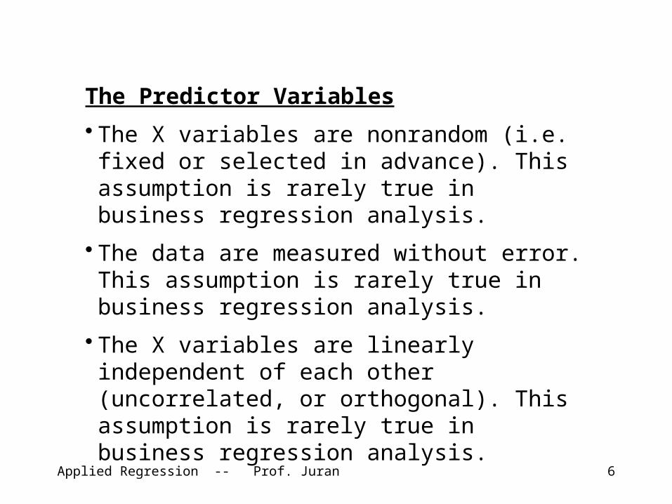
In the extreme case of exact dependence, the XTX matrix cannot be inverted and the regression procedure will fail. In less extreme cases, we suffer from several possible problems:1. The independent variables are not “independent”. We

can’t talk about the slope coefficients in terms of effects of one variable on Y “all other things held constant”, because changes in one of the X variables are associated with expected changes in other X variables.

2. The slope coefficient values can be very sensitive to changes in the data, and/or which other independent variables are included in the model.

3. Forecasting problems:• Large standard errors for all parameters• Uncertainty about whether true relationships have

been detected• Uncertainty about the stability of the correlation

structure


Sources of Collinearity

Data collection method. Some combination of X variable values does not exist in the data.

Example: Say that we did the tool wear case without ever trying the Type A machine at low speed or the Type B machine at high speed. Collinearity here is the result of the experimental design.



Constraints on the Model or in the Population. Some combination of X variable values does not exist in the population.

Example: In the cigarette data, imagine if the states with a high proportion of high school graduates also had a high proportion of black citizens. Collinearity here is the result of attributes of the population.



Model Specification. Adding or including variables that are tightly correlated with other variables already in the model.Example: In a study to predict the profitability of TV programs, we might include both the Nielsen rating and the Nielsen share. Collinearity here is the result of including multiple variables that contain more or less the same information.



Over-definition. We may have a relatively small number of observations, but a large number of independent variables for each.

Collinearity here is the result of too few degrees of freedom. In other words, n – p – 1 is small (or in the extreme, negative), because p is large compared with n.


Detecting Collinearity

First, be aware of the potential problem, and be vigilant.

Second, check the various combinations of independent variables for obvious evidence of collinearity. This might include pairwise correlation analysis, or even regressing each independent variable against all of the others. A high R-square coefficient would be a sign of trouble.


Detecting CollinearityThird, after a regression model has been estimated, watch for these clues:

Large changes in a coefficient as an independent variable is added or removed.

Large changes in a coefficient as an observation is added or removed.

Inappropriate signs or magnitudes of an estimated coefficient as compared to common sense or prior expectations.

The Variance Inflation Factor (VIF) is one measure of collinearity’s impact.


Variance Inflation FactorS u p p o s e t h a t i n d e p e n d e n t v a r i a b l e X j i s r e g r e s s e d a g a i n s t a l l o t h e r v a r i a b l e s , a n d t h e r e s u l t i n g R - s q u a r e v a l u e i s 2

jR . T h e V I F f o r v a r i a b l e j i s d e fi n e d a s

pjR

VIFj

j ,,2,1,1

12

N o t e t h a t i f t h e p r e d i c t o r v a r i a b l e s a r e o r t h o g o n a l , e a c h R - s q u a r e i s z e r o , a n d h e n c e e a c h V I F i s 1 . T h i s i s i d e a l , a n d c a n b e a c h i e v e d i n w e l l - d e s i g n e d e x p e r i m e n t s .

T h e s q u a r e r o o t o f t h e V I F i s a m e a s u r e o f t h e p r o p o r t i o n a l i n c r e a s e i n t h e w i d t h o f t h e c o n fi d e n c e i n t e r v a l f o r t h e s l o p e c o e ffi c i e n t f o r X j t h a t i s c a u s e d b y c o l l i n e a r i t y .

A r u l e o f t h u m b : a V I F o f g r e a t e r t h a n 5 i n d i c a t e s s e r i o u s t r o u b l e .


CountermeasuresDesign as much orthogonality into the data as you can. You may improve a pre-existing situation by collecting additional data, as orthogonally as possible.

Exclude variables from the model that you know are correlated.

Principal Components Analysis: Basically creating a small set of new independent variables, each of which is a linear combination of the larger set of original independent variables (Ch. 9.5, RABE).


Countermeasures

In some cases, rescaling and centering the data can diminish the collinearity. For example, we can translate each observation into a z-stat (by subtracting the mean and dividing by the standard deviation).

1

11

X

i

s

XX


Collinearity in the Supervisor Data

X1 X2 X3 X4 X5 X6

X1 1 0

10

20

30

40

50

60

70

80

90

0 10 20 30 40 50 60 70 80 90 100

X1

X2

0

10

20

30

40

50

60

70

80

0 10 20 30 40 50 60 70 80 90 100

X1

X3

0

10

20

30

40

50

60

70

80

90

100

0 10 20 30 40 50 60 70 80 90 100

X1

X4

0

10

20

30

40

50

60

70

80

90

100

0 10 20 30 40 50 60 70 80 90 100

X1

X5

0

10

20

30

40

50

60

70

80

0 10 20 30 40 50 60 70 80 90 100

X1

X6

X2 0.5583 1 0

10

20

30

40

50

60

70

80

0 10 20 30 40 50 60 70 80 90

X2

X3

0

10

20

30

40

50

60

70

80

90

100

0 10 20 30 40 50 60 70 80 90

X2

X4

0

10

20

30

40

50

60

70

80

90

100

0 10 20 30 40 50 60 70 80 90

X2

X5

0

10

20

30

40

50

60

70

80

0 10 20 30 40 50 60 70 80 90

X2

X6

X3 0.5967 0.4933 1 0

10

20

30

40

50

60

70

80

90

100

0 10 20 30 40 50 60 70 80

X3

X4

0

10

20

30

40

50

60

70

80

90

100

0 10 20 30 40 50 60 70 80

X3

X5

0

10

20

30

40

50

60

70

80

0 10 20 30 40 50 60 70 80

X3

X6

X4 0.6692 0.4455 0.6403 1 0

10

20

30

40

50

60

70

80

90

100

0 10 20 30 40 50 60 70 80 90 100

X4

X5

0

10

20

30

40

50

60

70

80

90

100

0 10 20 30 40 50 60 70 80 90 100

X4

X5

X5 0.1877 0.1472 0.1160 0.3769 1 0

10

20

30

40

50

60

70

80

0 10 20 30 40 50 60 70 80 90 100

X5

X6

X6 0.2246 0.3433 0.5316 0.5742 0.2833 1


L et’s look at the variance inflation factors in the full model and in the reduced model. H ere are the results of regressing X 1 on all other independent variables, and the calculation of the V IF for X 1:

3456789

1 01 11 21 31 41 51 61 71 81 92 02 12 2

H I J K L MR e gre ss io n S ta tis ticsM u ltip le R 0 .7 9 0 6 V IFR S q u are 0 .6 2 5 1 2 .6 6 7 1A d ju s ted R S q u are 0 .5 4 6 9S tan d ard E rror 8 .9 6 2 1O b servation s 3 0

A N O V Ad f S S M S F S ign ifica n ce F

R eg ress ion 5 3 2 1 3 .5 3 4 6 6 4 2 .7 0 6 9 8 .0 0 1 9 0 .0 0 0 1R es id u a l 2 4 1 9 2 7 .6 6 5 4 8 0 .3 1 9 4Total 2 9 5 1 4 1 .2 0 0 0

C o e ffic ie n ts S ta n d a rd E rro r t S ta t P -va lu eIn tercep t 4 .9 0 2 6 1 4 .6 6 0 9 0 .3 3 4 4 0 .7 4 1 0X 2 0 .3 1 5 4 0 .1 5 9 6 1 .9 7 6 4 0 .0 5 9 7X 3 0 .3 1 5 8 0 .2 0 3 7 1 .5 5 0 2 0 .1 3 4 2X 4 0 .7 1 6 7 0 .2 3 9 7 2 .9 8 9 5 0 .0 0 6 4X 5 -0 .0 0 0 9 0 .1 8 6 4 -0 .0 0 4 8 0 .9 9 6 2X 6 -0 .4 4 5 3 0 .2 0 6 9 -2 .1 5 2 2 0 .0 4 1 6

=1 /(1 -I5 )


Here is a summary of the VIFs for the full model: Regression Statistics Multiple R 0.8559 R Square 0.7326 Adjusted R Square 0.6628 Standard Error 7.0680 Observations 30 ANOVA df SS MS F Significance F Regression 6 3147.9663 524.6611 10.5024 0.0000 Residual 23 1149.0003 49.9565 Total 29 4296.9667 Coefficients Standard Error t Stat P-value VIF Intercept 10.7871 11.5893 0.9308 0.3616 X1 0.6132 0.1610 3.8090 0.0009 2.6671 X2 -0.0731 0.1357 -0.5382 0.5956 1.6009 X3 0.3203 0.1685 1.9009 0.0699 2.2710 X4 0.0817 0.2215 0.3690 0.7155 3.0782 X5 0.0384 0.1470 0.2611 0.7963 1.2281 X6 -0.2171 0.1782 -1.2180 0.2356 1.9516


For the reduced model: Regression Statistics Multiple R 0.8414 R Square 0.7080 Adjusted R Square 0.6864 Standard Error 6.8168 Observations 30 ANOVA df SS MS F Significance F Regression 2 3042.3177 1521.1588 32.7353 0.0000 Residual 27 1254.6490 46.4685 Total 29 4296.9667 Coefficients Standard Error t Stat P-value VIF Intercept 9.8709 7.0612 1.3979 0.1735 X1 0.6435 0.1185 5.4316 0.0000 1.5530 X3 0.2112 0.1344 1.5713 0.1278 1.5530


CarsRegression StatisticsMultiple R 0.9757R Square 0.9520Adjusted R Square 0.8859Standard Error 4435Observations 42

ANOVAdf SS MS F Significance F

Regression 16 10146131594 634133224.6 34.38 0.0000 Residual 26 511504646.2 19673255.62Total 42 10657636240

Coefficients Standard Error t Stat P-valueIntercept -13060 11651 -1.1209 0.2726MPG City 666.4 222.7 2.9920 0.0060HP 140.7 21.6 6.5264 0.0000Trunk -0.7 430.3 -0.0017 0.9986Powertrain Warranty (k miles) -69.7 97.4 -0.7159 0.4804Audi 7857 5279 1.4884 0.1487Chrysler 1770 4297 0.4120 0.6837Ford -4533 4292 -1.0561 0.3006Honda -1215 4455 -0.2727 0.7872Lexus 2386 5116 0.4663 0.6449Mazda 0.0000 0.0000 65535.0000 #NUM!Nissan -1692 3895 -0.4344 0.6676Saturn 1899 3891 0.4880 0.6297Toyota -2435 3991 -0.6101 0.5471Volkswagen -621 3808 -0.1631 0.8717RW D 7563 3842 1.9684 0.0598AWD 11443 4772 2.3978 0.0240


Regression StatisticsMultiple R 1.0000R Square 1.0000Adjusted R Square 1.0000Standard Error 0.0000Observations 42


Regression 13 4.404761905 0.338827839 1.04862E+31 0Residual 28 9.04731E-31 3.23118E-32Total 41 4.404761905

Coefficients Standard Error t Stat P-valueIntercept 2.500 0.000 5394870107975790.000 0.0000MPG City 0.000 0.000 -1.299 0.2047HP 0.000 0.000 -0.198 0.8448Trunk 0.000 0.000 1.519 0.1400Powertrain Warranty (miles) -0.025 0.000 -8210312317652900.000 0.0000Audi -1.250 0.000 -8082933516228270.000 0.0000Chrysler 0.000 0.000 -1.608 0.1191Ford -1.000 0.000 -7460122631949060.000 0.0000Honda -1.000 0.000 -6487369098305350.000 0.0000Lexus -0.750 0.000 -5518199114894210.000 0.0000Mazda -1.000 0.000 -6484199036307860.000 0.0000Nissan -1.000 0.000 -8248383048176410.000 0.0000Saturn 0.000 0.000 -1.309 0.2012Toyota -1.000 0.000 -8085329423437790.000 0.0000

New model: Dependent variable is Volkswagen.


Reduced Volkswagen model:



Regression 8 4.4048 0.5506 2604017745301400000000000000000 0.0000Residual 33 0.0000 0.0000Total 41 4.4048

Coefficients Standard Error t Stat P-valueIntercept 2.5 0.0000 4393622119841900 0.0000Warranty -0.025 0.0000 -3814732274639060 0.0000Audi -1.25 0.0000 -3768631097539650 0.0000Ford -1 0.0000 -2977874427443340 0.0000Honda -1 0.0000 -2599301899777600 0.0000Lexus -0.75 0.0000 -3293117056957300 0.0000Mazda -1 0.0000 -2599301899777600 0.0000Nissan -1 0.0000 -3241899051252790 0.0000Toyota -1 0.0000 -3438553204594630 0.0000




Regression 7 1.3278 0.1897 2.0961 0.0709Residual 34 3.0769 0.0905Total 41 4.4048

Coefficients Standard Error t Stat P-valueIntercept 0.3846 0.0834 4.610 0.0001Audi -0.3846 0.1583 -2.430 0.0206Ford -0.3846 0.1927 -1.996 0.0540Honda -0.3846 0.2285 -1.683 0.1015Lexus -0.3846 0.1352 -2.845 0.0075Mazda -0.3846 0.2285 -1.683 0.1015Nissan -0.3846 0.1720 -2.236 0.0320Toyota -0.3846 0.1583 -2.430 0.0206

42 cars in the data set, 29 represented by the dummy variables

above.

13 remaining, of which 5 are VW.


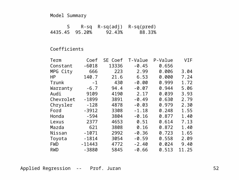
Some Minitab OutputRegression Analysis: MSRP versus MPG City, HP, Trunk, Warranty, Audi, Chevrolet, ...

The following terms cannot be estimated and were removed: Saturn, Volkswagen, AWD

Analysis of Variance

Source DF Adj SS Adj MS F-Value P-ValueRegression 15 10146131594 676408773 34.38 0.000 MPG City 1 176114556 176114556 8.95 0.006 HP 1 837954013 837954013 42.59 0.000 Trunk 1 58 58 0.00 0.999 Warranty 1 100549 100549 0.01 0.944 Audi 1 92960483 92960483 4.73 0.039 Chevrolet 1 4684125 4684125 0.24 0.630 Chrysler 1 13631 13631 0.00 0.979 Ford 1 27504490 27504490 1.40 0.248 Honda 1 479148 479148 0.02 0.877 Lexus 1 5133880 5133880 0.26 0.614 Mazda 1 523598 523598 0.03 0.872 Nissan 1 2520242 2520242 0.13 0.723 Toyota 1 6940256 6940256 0.35 0.558 FWD 1 113111527 113111527 5.75 0.024 RWD 1 8669257 8669257 0.44 0.513Error 26 511504646 19673256Total 41 10657636240

Adjusted sums of squares are the additional sums of squares determined by adding each particular term to the model given the other terms are already in the model.


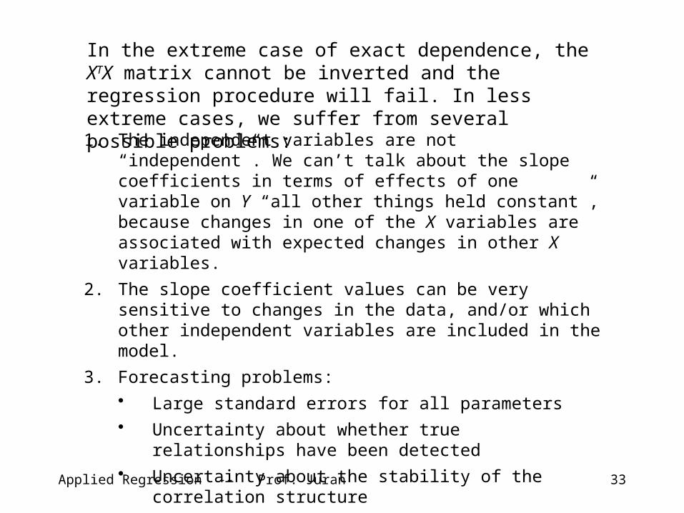
Model Summary

S R-sq R-sq(adj) R-sq(pred)4435.45 95.20% 92.43% 88.33%

Coefficients

Term Coef SE Coef T-Value P-Value VIFConstant -6018 13336 -0.45 0.656MPG City 666 223 2.99 0.006 3.04HP 140.7 21.6 6.53 0.000 7.24Trunk -1 430 -0.00 0.999 1.72Warranty -6.7 94.4 -0.07 0.944 5.06Audi 9109 4190 2.17 0.039 3.93Chevrolet -1899 3891 -0.49 0.630 2.79Chrysler -128 4878 -0.03 0.979 2.30Ford -3912 3308 -1.18 0.248 1.55Honda -594 3804 -0.16 0.877 1.40Lexus 2377 4653 0.51 0.614 7.13Mazda 621 3808 0.16 0.872 1.40Nissan -1071 2992 -0.36 0.723 1.65Toyota -1814 3054 -0.59 0.558 2.09FWD -11443 4772 -2.40 0.024 9.40RWD -3880 5845 -0.66 0.513 11.25


(A.k.a. Autocorrelation)

Here we are concerned with the assumption that the residuals are independent of each other.

In particular, we are suspicious that the sequential residuals have a positive correlation. In other words, some information about an observed value of the dependent variable is contained in the previous observation.

Serial Correlation


Consider the following historical data set, in which the dependent variable is Consumer Expenditure and the independent variable is Money Stock. (Economists are interested in the effect of Money Stock on Expenditure, because if it is significant it presents an opportunity to influence the economy through public policy.)

Year Quarter Expenditure Stock Year Quarter Expenditure Stock 1952 1 214.6 159.3 1954 3 238.7 173.9 1952 2 217.7 161.2 1954 4 243.2 176.1 1952 3 219.6 162.8 1955 1 249.4 178.0 1952 4 227.2 164.6 1955 2 254.3 179.1 1953 1 230.9 165.9 1955 3 260.9 180.2 1953 2 233.3 167.9 1955 4 263.3 181.2 1953 3 234.1 168.3 1956 1 265.6 181.6 1953 4 232.3 169.7 1956 2 268.2 182.5 1954 1 233.7 170.5 1956 3 270.4 183.3 1954 2 236.5 171.6 1956 4 275.6 184.3


Regression Statistics Multiple R 0.9784 R Square 0.9573 Adjusted R Square 0.9549 Standard Error 3.9827 Observations 20 ANOVA

df SS MS F Significance F Regression 1 6395.7666 6395.7666 403.2203 0.0000 Residual 18 285.5109 15.8617 Total 19 6681.2775

Coefficients Standard Error t Stat P-value Intercept -154.7192 19.8500 -7.7944 0.0000 Stock 2.3004 0.1146 20.0803 0.0000


Histogram of Residuals

0

1

2

3

4

5

6

7

8

-10 -8 -6 -4 -2 0 2 4 6 8 10

Residual Error

Fre

qu

en

cy


Line Fit Plot

200

210

220

230

240

250

260

270

280

200 210 220 230 240 250 260 270 280

Predicted Expenditure

Ex

pe

nd

itu

re


Normal Probability Plot

-3

-2

-1

0

1

2

3

-3 -2 -1 0 1 2 3

Normal Score

Sta

nd

ard

ize

d R

es

idu

al


Residual Plot vs. Money Stock

-8

-6

-4

-2

0

2

4

6

8

155 160 165 170 175 180 185 190

Stock

Re

sid

ua

ls


Residual Plot vs. Time

-8

-6

-4

-2

0

2

4

6

8

0 2 4 6 8 10 12 14 16 18 20

Time

Re

sid

ua

ls


Expenditure Time Stock Expenditure 1 0.9833 0.9784 Time 0.9833 1 0.9941 Stock 0.9784 0.9941 1


Run Chart of Expenditure

200

210

220

230

240

250

260

270

280

1 2 3 4 5 6 7 8 9 10 11 12 13 14 15 16 17 18 19 20

Time

Ex

pe

nd

itu

re


Summary• Residual Analysis• Are they normal?• Do they have a common variance?

• Multicollinearity• Autocorrelation, serial correlation


For Session 7• Practice the Excel array functions

– Do a full multiple regression model of the cigarette data:

www.ilr.cornell.edu/~hadi/RABE/Data/P081.txt

– Replicate the regression results using matrix algebra

– OK to e-mail this one to TAs• Artsy case

Session 6. Applied Regression -- Prof. Juran2 Outline Residual Analysis Are they normal? Do they...

Documents

Transcript of Session 6. Applied Regression -- Prof. Juran2 Outline Residual Analysis Are they normal? Do they...