Session 2b:

Wind power spatial

planning techniques

IRENA Global AtlasSpatial planning techniques

2-day seminar

Central questions we want to answer

• After having identified those areas which are potentially available for renewables, we

want to estimate…

� what the potential solar wind capacity per km² and in total is (W/km²), and,

� how much electricity (Wh/km²/a) can be generated in areas with different wind � how much electricity (Wh/km²/a) can be generated in areas with different wind

regimes.

• We also need to know which parameters are the most sensitive ones in order to identify

the most important input parameters.

2

Wind speed at hub height (m/s)

Wind speed extrapolation to turbine hub height

Roughness length or wind shear exponent

Hub height (m)

Energy output calculation

Power curve, wind turbine

Economic parameters

(wind farm and

apacity

expenditu

re, O

PE

X =

Opera

tion

eig

hte

d a

vera

ge c

ost of

Areas potentially suitable for wind farms (km2) Site assessment (wind atlas data, wind speed (m/s) for certain height (m))

Exclusion of non-suitable land areas and adding of buffer zones

Nature protected area

Transport, supply and

Areas technically not suitable (high slope and above certain altitude, etc.)

done

pen

din

g

3

© R

EN

AC

2014Energy generation costs at specific site (€/Wh)

Power curve, wind turbine density (W/km2), air density

Weibull distribution (k, A)

Electrical losses (%)

CAPEX

OPEX

WACC

Life time

(wind farm and grid connection)

Annual energy prod. (Wh/a/km2)Wind capacity per area (W/km2) C

AP

EX

= C

apacity

expenditu

re, O

PE

X =

Opera

tion

expenditu

re, W

AC

C =

Weig

hte

d a

vera

ge c

ost of

capita

l (depth

, equity

)

Urban area (buffer zone: 8–10 hub height)

Transport, supply and communication infrastructure

Landscape, historic area, other non-usable land (glaciers, rivers, etc.)

Areas potentially suitable for wind farms (km2)

Priority areas for wind power (km2), potentially installed capacity (W), potentially

generated energy (Wh/a) and costs

Energy policy analysis

Economic assessment

done

pen

din

g

Agenda

1. Overview on wind energy estimation

2. Formation of wind

3. Technical aspects we need to know

4. Spatial setup of wind farms4. Spatial setup of wind farms

5. Estimating wind electricity yield

6. Worked example: Estimating wind capacity and yield at a given site

4

1. OVERVIEW ON WIND

ENERGY ESTIMATION

5

Wind speed extrapolation

Extrapolated wind speed

6

Height of measuredwind speed

Extrapolated wind speedat hub height

Wind speed extrapolation also depends on

surroundings

Extrapolated wind speed

7

Height of measuredwind speed

Extrapolated wind speedat hub height

Each turbine type has its characteristic power

curve

8

At each site, wind has its own timely distribution

Site AAverage wind speed data isnot sufficient, wind speed

distribution is crucial!

9

Site B

Estimating wind energy generation

• Estimation of wind energy generation depends on a large number of factors and should

be carried out with great care.

• It is necessary to find a representative mix of suitable wind turbines in order to get a

good estimate of the wind energy that could be produced.good estimate of the wind energy that could be produced.

• If there is, the resulting capacity factor (full-load hours) should be cross-checked with

existing wind projects.

• If there already is a larger number of wind projects, one could alternatively use existing

capacity factor information for further estimations.

• If data is not available a national measurement campaign may be advisable.

10

Wind measurement tube towers

Source: http://www.energieprojekte.de/en/index.html11

2. FORMATION OF WIND

12

High and low pressure area

• High pressure area occurs when air becomes colder (winter high pressure areas can be quite strong and lasting). The air become heavier and sink towards the earth. heavier and sink towards the earth. Skies are usually clear. The airflow is clockwise (northern hemi). The air flows towards the low pressure area over the ground.

Source: http://www.experimentalaircraft.info/weather/weather-info-1.phpar

Isobars

• Low pressure occurs when air becomes warmer. The air become lighter and rises. The pressure lowers towards the center and air flow is counterclockwise (northern hemi). Clouds will appear due to rising of the moist warm air and the weather will deteriorate. Air will flow back to the high pressure area at higher altitudes in the atmosphere.

13

Mountain valley breeze

14

Sea-land breeze

15

3. TECHNICAL ASPECTS

WE NEED TO KNOW

16

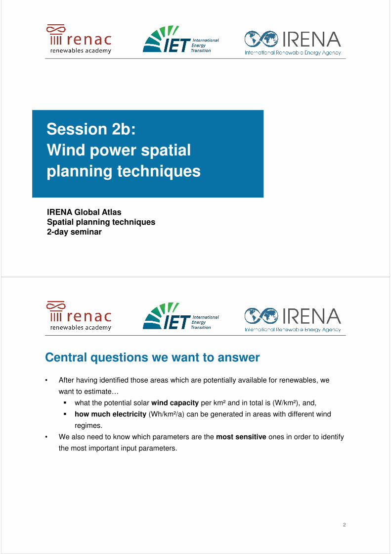
Vertical wind shear profile and roughness of

surface H

eig

ht

Heig

ht

Profile above area with low roughness (sea, low grass)

Heig

ht

Heig

ht

Profile above area with high roughness (forest, town) 17

Roughness length Z0 and wind shear

• To evaluate wind conditions in a landscape information on the roughness is needed.

The roughness classes or roughness lengths are specific for different landscapes.

• Wind shear: The fact that the wind profile is twisted towards a lower speed as we move

closer to ground level, is usually called wind shear.closer to ground level, is usually called wind shear.

Source: http://www.windpower.org/en/core.htma

18

Roughness classes and roughness lengths

(European wind atlas)

Rough-ness class

Roughnesslength Z0 [m]

Landscape type

0 0.0002 Water surface

0.5 0.0024 Completely open terrain with a smooth surface, e.g. concrete runways in airports, mowed grass, etc.

0.5 0.0024 airports, mowed grass, etc.

1 0.03 Open agricultural area without fences and hedgerows and very scattered buildings. Only softly rounded hills

1.5 0.055 Agricultural land with some houses and 8 meters tall sheltering hedgerows with a distance of approx. 1250 meters

2 0.1 Agricultural land with some houses and 8 meters tall sheltering hedgerows with a distance of approx. 500 meters

2.5 0.2 Agricultural land with many houses, shrubs and plants, or 8 metre tall sheltering hedgerows with a distance of approx. 250 meters

3 0.4 Villages, small towns, agricultural land with many or tall sheltering hedgerows, forests and very rough and uneven terrain

3.5 0.8 Larger cities with tall buildings

4 1.6 Very large cities with tall buildings and skyscrapers 19

Calculating wind speed at different heights

h2

�2 = �1 ∗ln(

ℎ2

�0)

ln(ℎ1

�0)

h1

Where:

h1 : height [m]

h2 : height [m]

v1 : wind speed at h1 [m/s]

v2 : wind speed at h2 [m/s]

z0 : roughness length [m]

�2 = �1 ∗ln(

�0)

ln(ℎ1

�0)

20

Sample wind speeds at different heights

� Wind speed increases with height above ground

21

ground

� Profile depends on surface properties (roughness length, Z0)

Site specific wind resource assessment for wind

farm planning• To calculate the annual energy production of

a wind turbine the distribution of wind speeds

is needed. It can be approximated by a

Weibull equation with parameters A and K)

hw(v

)

Weibull equation with parameters A and K)

• The distribution of wind directions is important

for the siting of wind turbines in a wind farm.

The wind rose shows probability of a wind

from a certain sector.

• Wind speed distributions are measured for

different wind direction sectors.

22

Weibull values at 50m, Canada**

PeriodMean Wind

Speed

Wind Power

density

Weibull shape

parameter (k)

Weibull scale

parameter (A)

Annual 9.22 m/s 831 W/m2 1.81 10.37 m/s

Winter (DJF) 10.43 m/s 1119W/m2 1.94 11.76 m/s

Spring (MAM) 9.03 m/s 762 W/m2 1.85 10.16 m/s

Summer (JJA) 7.86 m/s 473 W/m2 1.96 8.87 m/s

Fall (SON) 9.44 m/s 827 W/m2 1.94 10.65 m/s

Source:, http://www.windatlas.ca/en/maps.php?field=E1&height=80&season=ANU

**) Location: latitude = 50.853, longitude = -57.007

23

Weibull equation factors for different regions

• For regions with similar topography the k factors are also similar

� 1.2 < k < 1.7 Mountains

� 1.8 < k < 2.5 Typical North America and Europe

� 2.5 < k < 3.0 Where topography increases wind speeds� 2.5 < k < 3.0 Where topography increases wind speeds

� 3.0 < k < 4.0 Winds in monsoon regions

• Scaling factor A is related to mean wind speed ( vavg ~ 0,8…0,9 · A)

• Relation of mean wind vavg, k und A (mean wind vavg, calculation)

• Warning: Only rough values! – On site monitoring is necessary !

Source: J.liersch; KeyWindEnergy, 2009

24

Wind measurements

• Synop measurements of meteorological stations at 10m above ground are often of

limited accuracy and use for wind energy applications

• Dedicated 50m masts with at least 3 sensors at different heights are much more • Dedicated 50m masts with at least 3 sensors at different heights are much more

expensive but much better suited to derive data for wind energy.

• Most such measurements are operated privately and data may not be accessible.

25

Wind Atlas based on modeling

• A suitable number of high quality

measurements is characterized for its local

effects

• The measurements are combined into an

atlasatlas

• Sample: 3TIER’s Global Wind Dataset 5km

onshore wind speed at 80m height units in

m/s

• Limitations for complex terrain and costal

zones

26

Map: IRENA Global Atlas; Data: 3TIER’s Global WindDataset

Power of wind

P = ½ x ρ x A x v3

� P = power of wind (Watt)

� ρ = air density (kg/m3; kilogram per cubic meter)

27

� A = area (m2; square meter)

� v = wind speed (m/s; meter per second)

Quick exercise: doubling of wind speed

• Let's double the wind speed and calculate what happens to the power of the swept rotor

area. Assume length of rotor blades (radius) 25 m and air density 1.225 kg/m^3).

• wind speed = 5 m wind speed = 10 m

28

Solution: doubling of wind speed

• Power of swept rotor calculated with 25 m rotor radius and 1.225 kg/m^3 air density

• wind speed = 5 m/s wind speed = 10 m/s

power = 150 kW power = 1200 kW

• Doubling of wind speed increases power by factor 8.• Doubling of wind speed increases power by factor 8.

• Calculation:

Power =0,5 * air density * (wind speed)^3 * blade length^2 * 3.1415

Power = 0,5 * 1,225 kg/m^3 * 5^3 m^3/s^3 * 25^2 m^2 * 3.1415 = 150 kW

Power = 0,5 * 1,225 kg/m^3 * 10^3 m^3/s^3 * 25^2 m^2 * 3.1415 = 1202.6 kW

Units:[kg/m^3 * ^3 m^3/s^3 * m^2 = Joule/s = W] 29

4. SPATIAL SETUP OF

WIND FARMS

30

Development wind turbine rotor diameter and hub height

75 m blade, Siemens (year 2012)

81.6 m blade, Mitsubishi80 m blade, Vestas (year 2013)

83.5 m blade, Samsung (year 2014)

31

60 m blade, Enercon (year 2008)

Swept area by rotor blades

A = π x (½ D) ²� A= swept rotor area [m] ²

� D = rotor diameter [m]

� π = 3.1415

D

� π = 3.1415

� The power output of a wind turbine is directly related to the area swept by the rotor blades. The larger thediameter of its rotor blades, the more power the wind turbine can extract from the wind. The swept area is also called the 'capture area'.

� The rotor diameter of most wind turbines is listed in specification sheets.

32

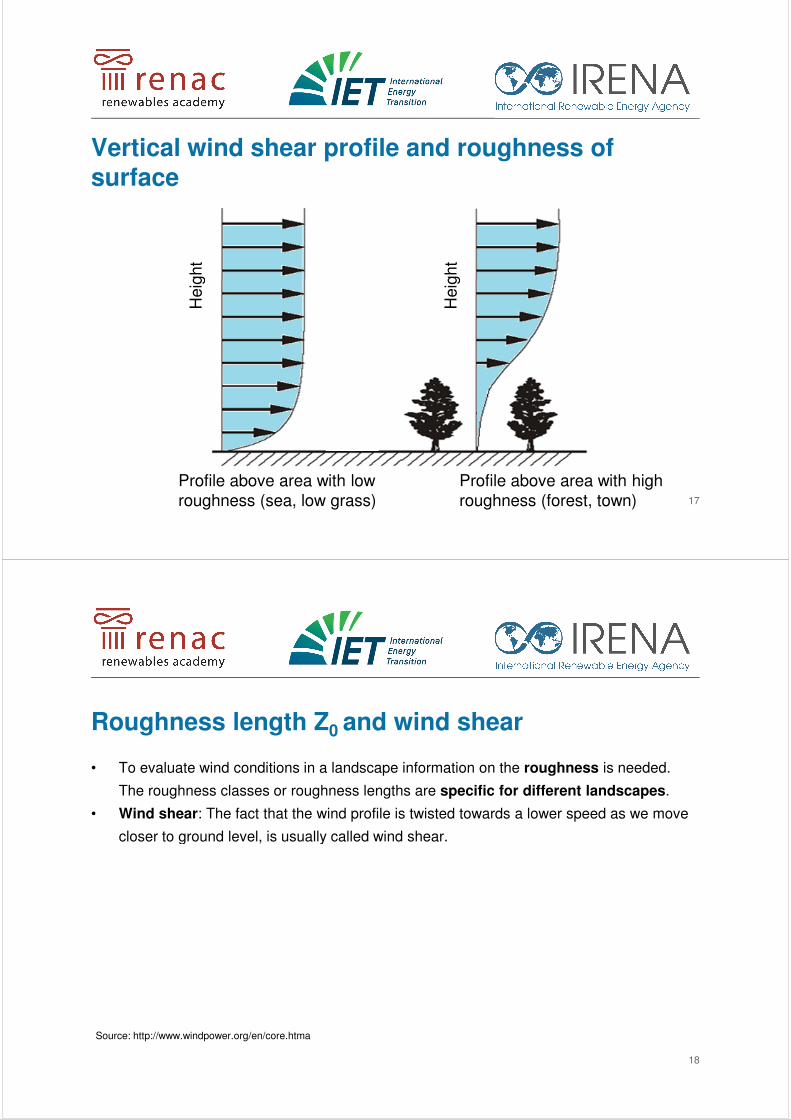
Wake effect

� Clouds form in the wake of the front row of wind turbines at the Horns Rev offshore wind farm in the North Sea

� Back-row wind turbines losing power relative to the front row Source: www.popsci.com/technology/article/2010-01/wind-turbines-leave-clouds-and-energy-inefficiency-their-wake

33

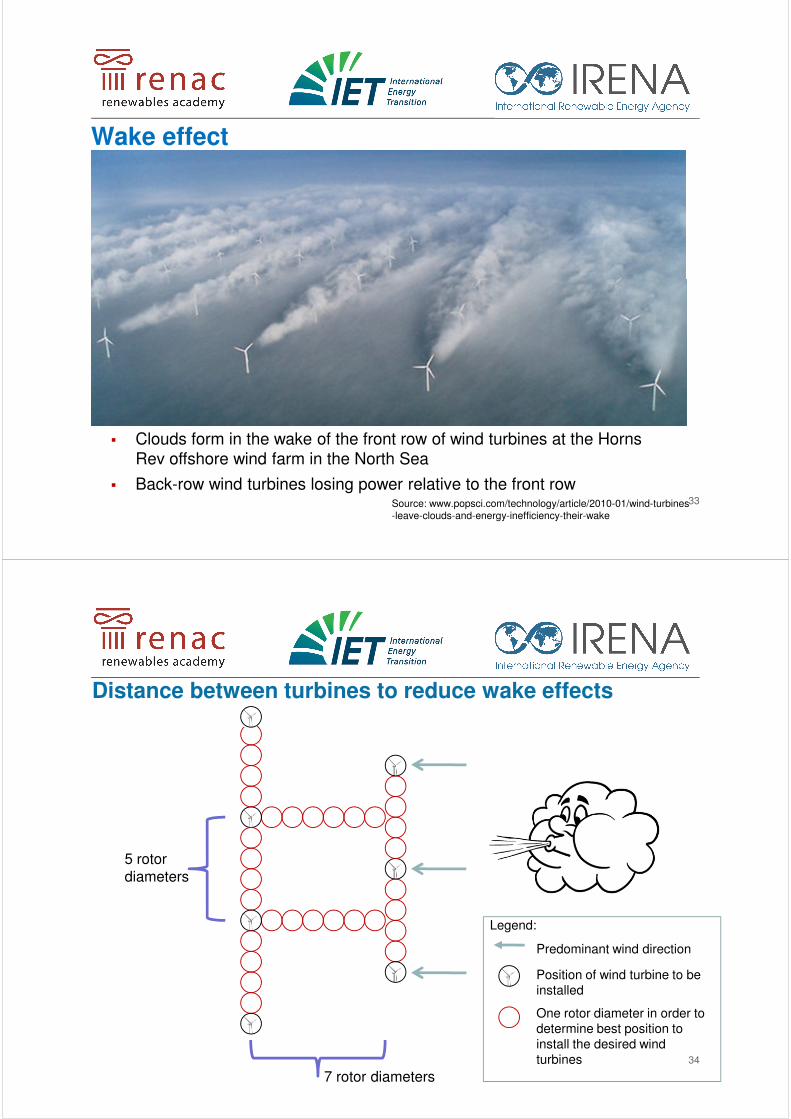
Distance between turbines to reduce wake effects

Legend:

Predominant wind direction

Position of wind turbine to beinstalled

One rotor diameter in order todetermine best position toinstall the desired wind turbines

5 rotordiameters

7 rotor diameters34

Generator capacity, W

Rotor diameter, m

Specific capacity, W/m^2

Wind turbine manufacturer

2300 113 230 SIEMENS SWT 2,3-133

2400 117 236 Nordex N100/2400

3000 126 241 Vestas V90-2MW

3200 114 314 REPOWER 3,2M-114

2000 90 314 Vestas V126-3MW

2500 100 318 Nordex N100/2500

1500 77 322 REPOWER MD77

2300 93 338 SIEMENS SWT 2,3-93

2300 82 436 Enercon E82-2,3

3000 82 568 Enercon E82-3,0

35

Specific power of today‘s wind turbines (generatorcapacity devided by sweapt rotor area)

Source: Molly, 2011 36

Wind power capacity and annual energy generation

estimation for an area e.g. with 25 km²

Rated power of wind turbine, MW 2 3 2 2,5 2,35 2,3 3

Rotor diameter of wind turbine, m 114 126 90 100 92 82 82

Specific rated power per swept rotor area (W/m^2)

196 241 314 318 354 436 568area (W/m^2)

Specific wind power capacity per land area, MW/ km^2; ***)

4,40 5,40 7,05 7,14 7,93 9,77 12,75

Number of turbines in the area 55 45 88 71 84 106 106

Installed wind power capacity, MW 110 135 176 179 198 244 319

Annual energy production with capacity factor of 0,35; GWh/a

337 414 541 548 608 749 977

37Source: RENAC calculation

***) Assumptions: distance between wind turbines standing in main wind direction:7 rotor diameter; and standing in in rarely ocurring perpendicular wind direction: 5 times the rotor diameter

5. ESTIMATING WIND

ELECTRICITY YIELD

38

What needs to be done

1. Define a representative mix of suitable turbines (potenitally site-specific).

2. Get power curve information for all turbine types.

3. Extrapollate average wind speeds to applicable hub heights.

4. Choose the wind speed distribution curve which is most likely at given sites(s).4. Choose the wind speed distribution curve which is most likely at given sites(s).

5. Calculate wind speed distributions for given hub heights.

6. Use wind speed distributions and power curves to calclulate representative wind energy

yield(s).

39

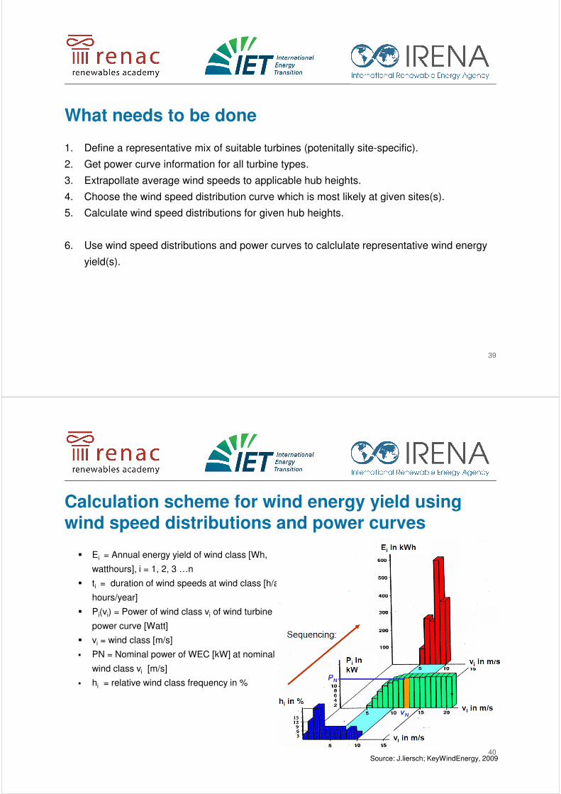
Calculation scheme for wind energy yield using

wind speed distributions and power curves

� Ei = Annual energy yield of wind class [Wh,

watthours], i = 1, 2, 3 …n

� ti = duration of wind speeds at wind class [h/a,

hours/year]hours/year]

� Pi(vi) = Power of wind class vi of wind turbine

power curve [Watt]

� vi = wind class [m/s]

� PN = Nominal power of WEC [kW] at nominal

wind class vi [m/s]

� hi = relative wind class frequency in %

Source: J.liersch; KeyWindEnergy, 200940

Calculation scheme for annual energy production

Ei = Pi(vi) * ti

EΣ = E1 + E2 +…+ En

� EΣ = Energy yield over one year

41

J.lie

rsch; K

eyW

indE

nerg

y, 2

009

Shape of different wind speed distributions

• Weibull distribution: shape factor k=1,25 andA= 8 m/s

42

• Weibull distribution: shape factor k=3 and A= 8 m/s

Sample power curves of wind turbines

(82 m rotor diameter, 2 and 3 MW)

Sourc

e: E

nerc

on p

roduct

info

rmatio

n2014

43

6. ESTIMATING WIND

CAPACITY AND YIELD AT A

GIVEN SITE

Worked example

44

Wind energy yield estimation near Arusha

• Steps performed:

1) Retrieve average wind speed data from

Global Atlas

2) Estimate electricity yield of one wind 2) Estimate electricity yield of one wind

turbine

3) Estimate wind power capacity and

potential wind energy per km² at given

location

45

Retrieving average wind speed

• Average wind speed 7.2 m/s at 80 m height

46

Extrapolation to hub height

• Wind data provided for height: h1 = 80 m

• Let‘s choose hub height: h2 = 90 m

• Roughness length: z0 = 0.1m

h2

h1

• Result: v2 = 7.3 m/s

47

Where:

h1 : height [m]

h2 : height [m]

v1 : wind speed at h1 [m/s]

v2 : wind speed at h2 [m/s]

z0 : roughness length [m]

Rough- nessclass

Roughnesslength Z0

[m]Landscape type

2 0.1

Agricultural land with some houses and 8 meters tall sheltering hedgerows with a distance of approx. 500 meters

�2 = �1 ∗ln(

ℎ2

�0)

ln(ℎ1

�0)

Estimating wind speed distribution

• Deriving Weibull distribution

� Average wind speed: v2 = vavg = 7.2 m/s

� Assumption: monsoon climate � k = 3.5

� Scaling factor: vavg = 0.9 * A � A = vavg / 0.9 � Scaling factor: vavg = 0.9 * A � A = vavg / 0.9

A = (vavg / 0.9) = (7.3 m/s) / 0.9 = 8.11 m/s

48

Resulting wind distribution

vi (m/s)Weibull probability (%)

number of

hours at vi m/s

per year0.0 0 0.01.0 0.002301447 20.22.0 0.012930901 113.33.0 0.03481178 305.04.0 0.067742212 593.4

49

4.0 0.067742212 593.45.0 0.107112259 938.36.0 0.14337442 1,256.07.0 0.164325824 1,439.58.0 0.160762789 1,408.39.0 0.132719153 1,162.6

10.0 0.090914034 796.411.0 0.05061706 443.412.0 0.022370894 196.013.0 0.007647482 67.014.0 0.001966378 17.215.0 0.000369182 3.216.0 4.90543E-05 0.417.0 4.46477E-06 0.0

Choosing the wind turbine

• We choose enercon E82-2000

vi (m/s)

Output power

of E82-2000,

(kW)

0.00

50

E82-2000

1.0 0

2.0 3

3.0 25

4.0 82

5.0 174

6.0 321

7.0 532

8.0 815

9.0 1180

10.0 1612

11.0 1890

12.0 2000

13.0 2050

14.0 2050

15.0 2050

16.0 2050

17.0 2050

Calculate power output per wind speed class

vi (m/s)

number of

hours at vi

m/s per

year

Output

power of

E82-2000,

(kW)

E82-2000,

annual energy yield, (kWh/a)

0.0 0.01.0 20.2 0 0

Example:@ v=7.0 m/s:1,439.5 h/a * 532 kW = 765,811 kWh/a

Total energy:1.0 20.2 0 02.0 113.3 3 3403.0 305.0 25 7,6244.0 593.4 82 48,6615.0 938.3 174 163,2656.0 1,256.0 321 403,1637.0 1,439.5 532 765,8118.0 1,408.3 815 1,147,7509.0 1,162.6 1180 1,371,891

10.0 796.4 1612 1,283,80811.0 443.4 1890 838,03612.0 196.0 2000 391,93813.0 67.0 2050 137,33314.0 17.2 2050 35,31215.0 3.2 2050 6,63016.0 0.4 2050 88117.0 0.0 2050 80

51

Total energy:Summation overall wind classes= 6.603 MWh/a

Estimating capacity per km²

• Rotor diameter d=82 m

• Distance d1 primary wind direction:

7 rotor diameters = 7 * 82 m = 574 m

• Distance d2 secondary wind direction:• Distance d2 secondary wind direction:

5 rotor diameters = 5 * 82 m = 410 m

• Area needed for one turbine:

574 m * 410 m = 235,340 m² = 0.24 km²

• Capacity per km²:

2 MW/0.24 km² = 8.3 MW/km²

52

Estimating energy per km² and capacity factor

• Capacity per km²:

2 MW/0.24 km² = 8.3 MW/km²

• Energy generation per wind turbine:

6,603 MWh per turbine (E82-2000) with 2 MW rated capacity,6,603 MWh per turbine (E82-2000) with 2 MW rated capacity,

OR: 6,603 MWh / 2 MW � 3,302 MWh / 1 MW

• Energy generated per km²:

3,302 MWh/MW * 8.3 MW/km² = 27,4 GWh/km²/a

• Capacity Factor: 3,302 MWh / 1 MW = 3,302 h

3,302 h / 8,760 h = 37.7%

53

Please remember

• The previous worked example is only a rough estimate and results are only true for the

given assumptions (specific site, one turbine type, wind distribution assumptions, etc.)

• The calculated energy yield should be considered as ideal result. In real-life power output

is likely to be slightly below these values due to downtimes (maintenance, grid outages), is likely to be slightly below these values due to downtimes (maintenance, grid outages),

cabling and transformation losses, deviation from ideal distribution of wind turbines on

the given site, etc.

54

Wind speed at hub height (m/s)

Wind speed extrapolation to turbine hub height

Roughness length or wind shear exponent

Hub height (m)

Energy output calculation

Power curve, wind turbine

Economic parameters

(wind farm and

apacity

expenditu

re, O

PE

X =

Opera

tion

eig

hte

d a

vera

ge c

ost of

Areas potentially suitable for wind farms (km2) Site assessment (wind atlas data, wind speed (m/s) for certain height (m))

Exclusion of non-suitable land areas and adding of buffer zones

Nature protected area

Transport, supply and

Areas technically not suitable (high slope and above certain altitude, etc.)

done

pen

din

g

done

55

© R

EN

AC

2014Energy generation costs at specific site (€/Wh)

Power curve, wind turbine density (W/km2), air density

Weibull distribution (k, A)

Electrical losses (%)

CAPEX

OPEX

WACC

Life time

(wind farm and grid connection)

Annual energy prod. (Wh/a/km2)Wind capacity per area (W/km2) C

AP

EX

= C

apacity

expenditu

re, O

PE

X =

Opera

tion

expenditu

re, W

AC

C =

Weig

hte

d a

vera

ge c

ost of

capita

l (depth

, equity

)

Urban area (buffer zone: 8–10 hub height)

Transport, supply and communication infrastructure

Landscape, historic area, other non-usable land (glaciers, rivers, etc.)

Areas potentially suitable for wind farms (km2)

Priority areas for wind power (km2), potentially installed capacity (W), potentially

generated energy (Wh/a) and costs

Energy policy analysis

Economic assessment

done

pen

din

g

done

Thank you very much for your Thank you very much for your

attention!

Jens Altevogt

Renewables Academy (RENAC)

Phone +49 30 52 689 58-76altevogt@renac.dewww.renac.de