
Session 2 Numerical Python and plotting - Steven...
40
Session 2: Numerical Python and plotting An introduction to scientific programming with
Transcript of Session 2 Numerical Python and plotting - Steven...
Session 2:Numerical Python and plotting
An introduction to scientific programming with

In this session:• Supplementary info for session 1
• IPython notebooks
• Session 1 exercise solutions
• Proper numerical arrays
• Plotting
• Exercises
Any questions?• shout and wave (now)
• tweet @thebamf (now)
• email [email protected] (later)
Session 2
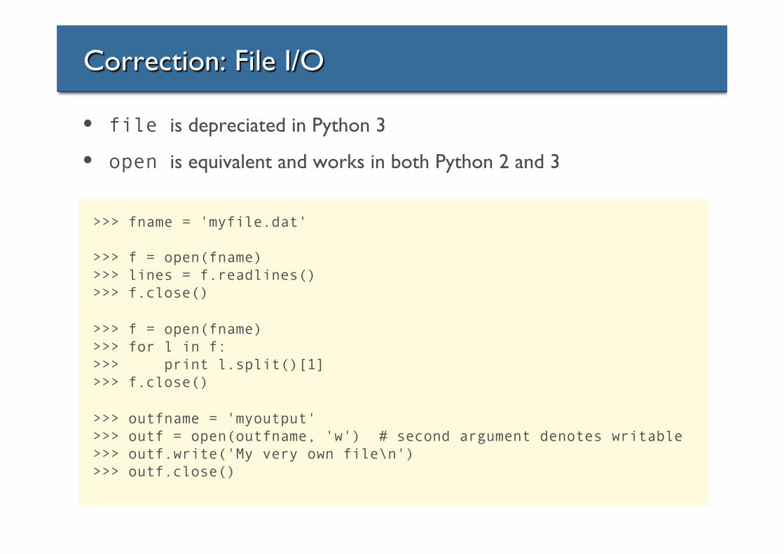
Correction: File I/O
>>> fname = 'myfile.dat' >>> f = open(fname) >>> lines = f.readlines() >>> f.close() >>> f = open(fname) >>> for l in f: >>> print l.split()[1] >>> f.close() >>> outfname = 'myoutput' >>> outf = open(outfname, 'w') # second argument denotes writable >>> outf.write('My very own file\n') >>> outf.close()
• file is depreciated in Python 3
• open is equivalent and works in both Python 2 and 3
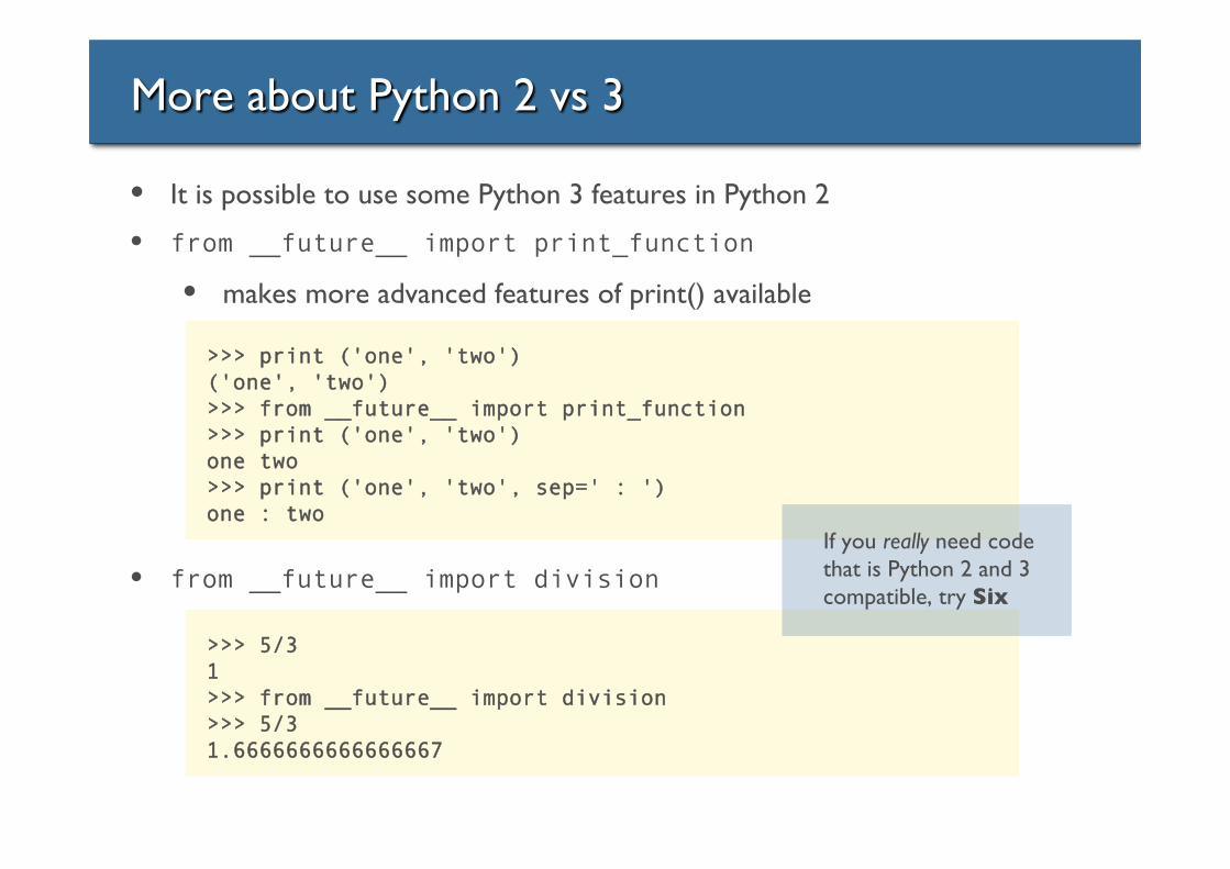
More about Python 2 vs 3
• It is possible to use some Python 3 features in Python 2
• from __future__ import print_function
• makes more advanced features of print() available
• from __future__ import division
>>> print ('one', 'two') ('one', 'two') >>> from __future__ import print_function >>> print ('one', 'two') one two >>> print ('one', 'two', sep=' : ') one : two
>>> 5/3 1 >>> from __future__ import division >>> 5/3 1.6666666666666667
If you really need code that is Python 2 and 3 compatible, try Six
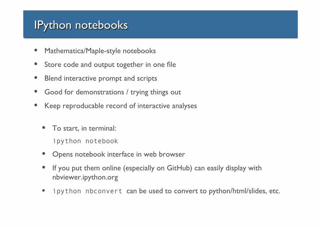
IPython notebooks
• Mathematica/Maple-style notebooks
• Store code and output together in one file
• Blend interactive prompt and scripts
• Good for demonstrations / trying things out
• Keep reproducable record of interactive analyses
• To start, in terminal:
ipython notebook
• Opens notebook interface in web browser
• If you put them online (especially on GitHub) can easily display with nbviewer.ipython.org
• ipython nbconvert can be used to convert to python/html/slides, etc.

Session 1 exercise solutions
[link to online notebook]
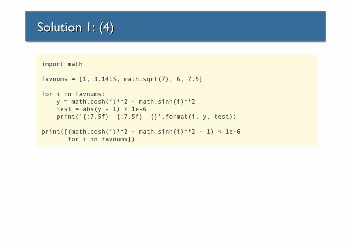
Solution 1: (4)
import math favnums = [1, 3.1415, math.sqrt(7), 6, 7.5] for i in favnums: y = math.cosh(i)**2 - math.sinh(i)**2 test = abs(y - 1) < 1e-6 print('{:7.5f} {:7.5f} {}'.format(i, y, test)) print([(math.cosh(i)**2 - math.sinh(i)**2 - 1) < 1e-6 for i in favnums])
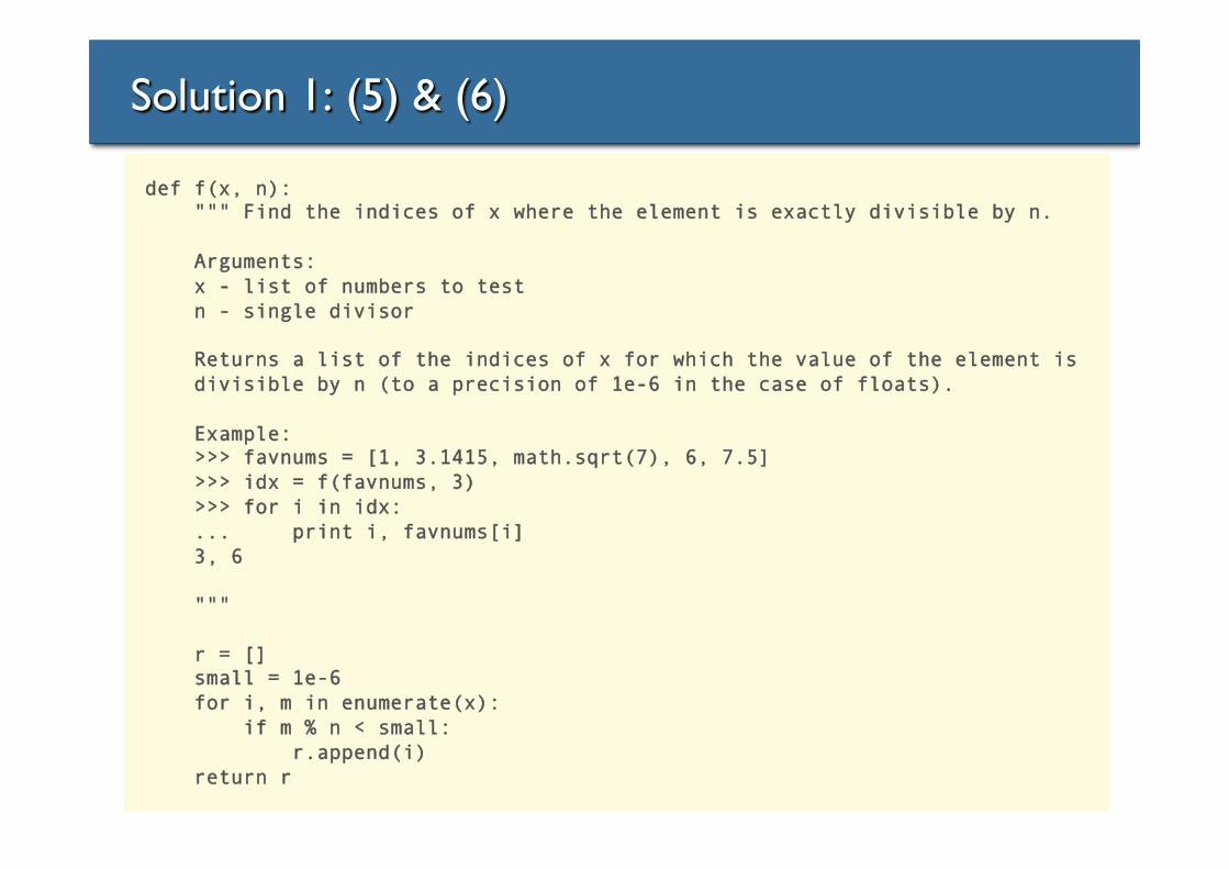
Solution 1: (5) & (6)
def f(x, n): """ Find the indices of x where the element is exactly divisible by n. Arguments: x - list of numbers to test n - single divisor Returns a list of the indices of x for which the value of the element is divisible by n (to a precision of 1e-6 in the case of floats). Example: >>> favnums = [1, 3.1415, math.sqrt(7), 6, 7.5] >>> idx = f(favnums, 3) >>> for i in idx: ... print i, favnums[i] 3, 6 """ r = [] small = 1e-6 for i, m in enumerate(x): if m % n < small: r.append(i) return r
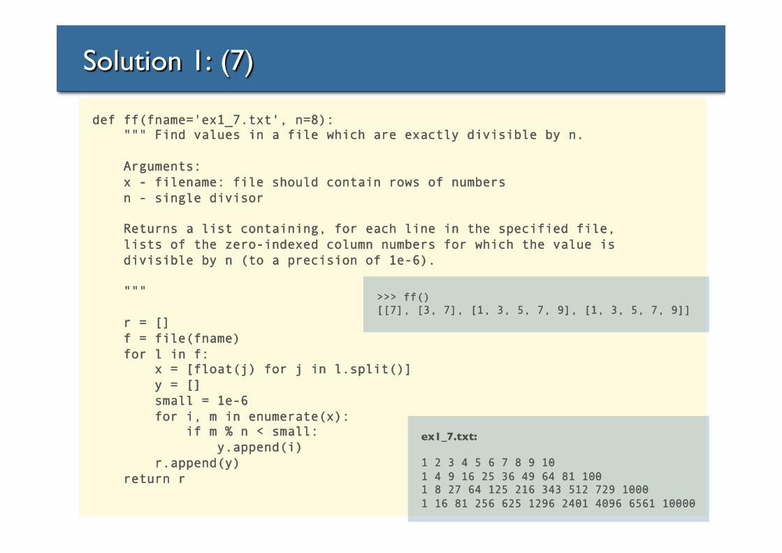
Solution 1: (7)
def ff(fname='ex1_7.txt', n=8): """ Find values in a file which are exactly divisible by n. Arguments: x - filename: file should contain rows of numbers n - single divisor Returns a list containing, for each line in the specified file, lists of the zero-indexed column numbers for which the value is divisible by n (to a precision of 1e-6). """ r = [] f = file(fname) for l in f: x = [float(j) for j in l.split()] y = [] small = 1e-6 for i, m in enumerate(x): if m % n < small: y.append(i) r.append(y) return r
ex1_7.txt:
1 2 3 4 5 6 7 8 9 10 1 4 9 16 25 36 49 64 81 100 1 8 27 64 125 216 343 512 729 1000 1 16 81 256 625 1296 2401 4096 6561 10000
>>> ff() [[7], [3, 7], [1, 3, 5, 7, 9], [1, 3, 5, 7, 9]]
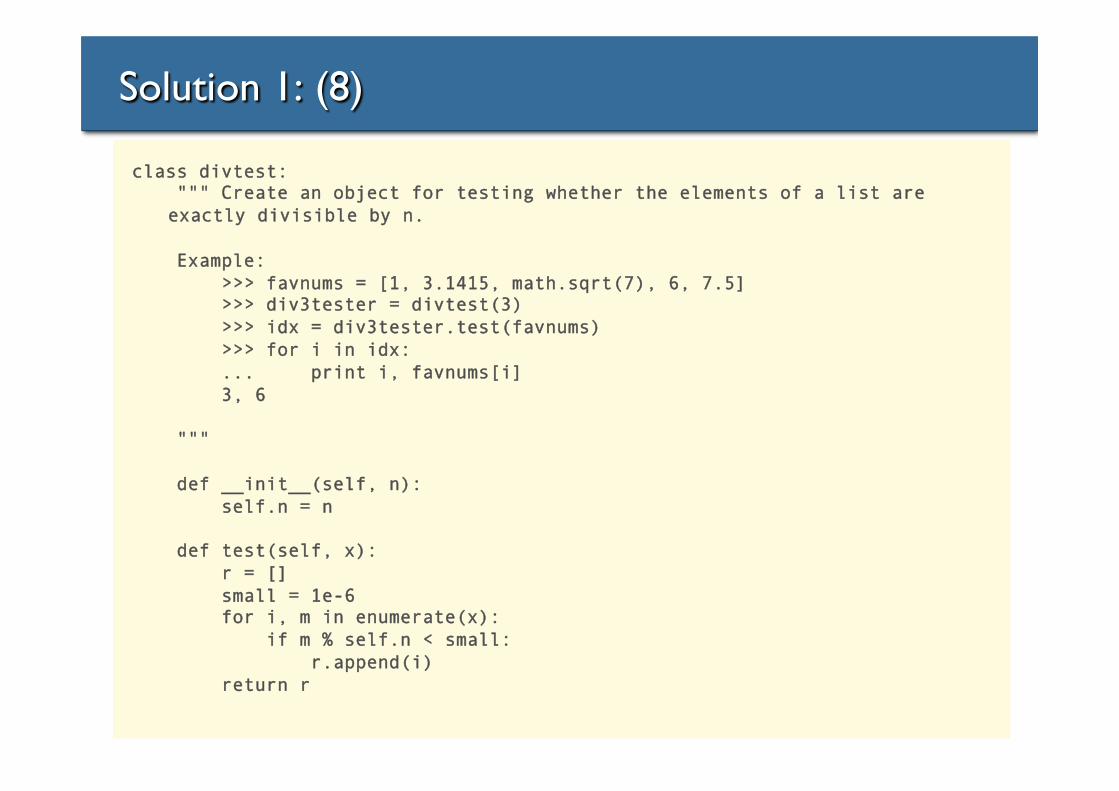
Solution 1: (8)
class divtest: """ Create an object for testing whether the elements of a list are
exactly divisible by n. Example: >>> favnums = [1, 3.1415, math.sqrt(7), 6, 7.5] >>> div3tester = divtest(3) >>> idx = div3tester.test(favnums) >>> for i in idx: ... print i, favnums[i] 3, 6 """ def __init__(self, n): self.n = n def test(self, x): r = [] small = 1e-6 for i, m in enumerate(x): if m % self.n < small: r.append(i) return r
Numerical Python
• So far…
• core Python language and libraries
• Extra features required:
• fast, multidimensional arrays
• plotting tools
• libraries of fast, reliable scientific functions (next session)
Arrays – Numerical Python (Numpy)
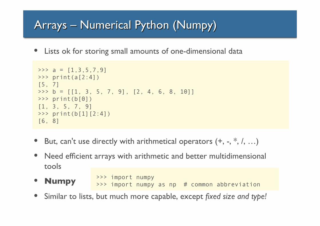
• Lists ok for storing small amounts of one-dimensional data
• But, can't use directly with arithmetical operators (+, -, *, /, …)
• Need efficient arrays with arithmetic and better multidimensional tools
• Numpy
• Similar to lists, but much more capable, except fixed size and type!
>>> a = [1,3,5,7,9] >>> print(a[2:4]) [5, 7] >>> b = [[1, 3, 5, 7, 9], [2, 4, 6, 8, 10]] >>> print(b[0]) [1, 3, 5, 7, 9] >>> print(b[1][2:4]) [6, 8]
>>> import numpy >>> import numpy as np # common abbreviation
Numpy – array creation and use
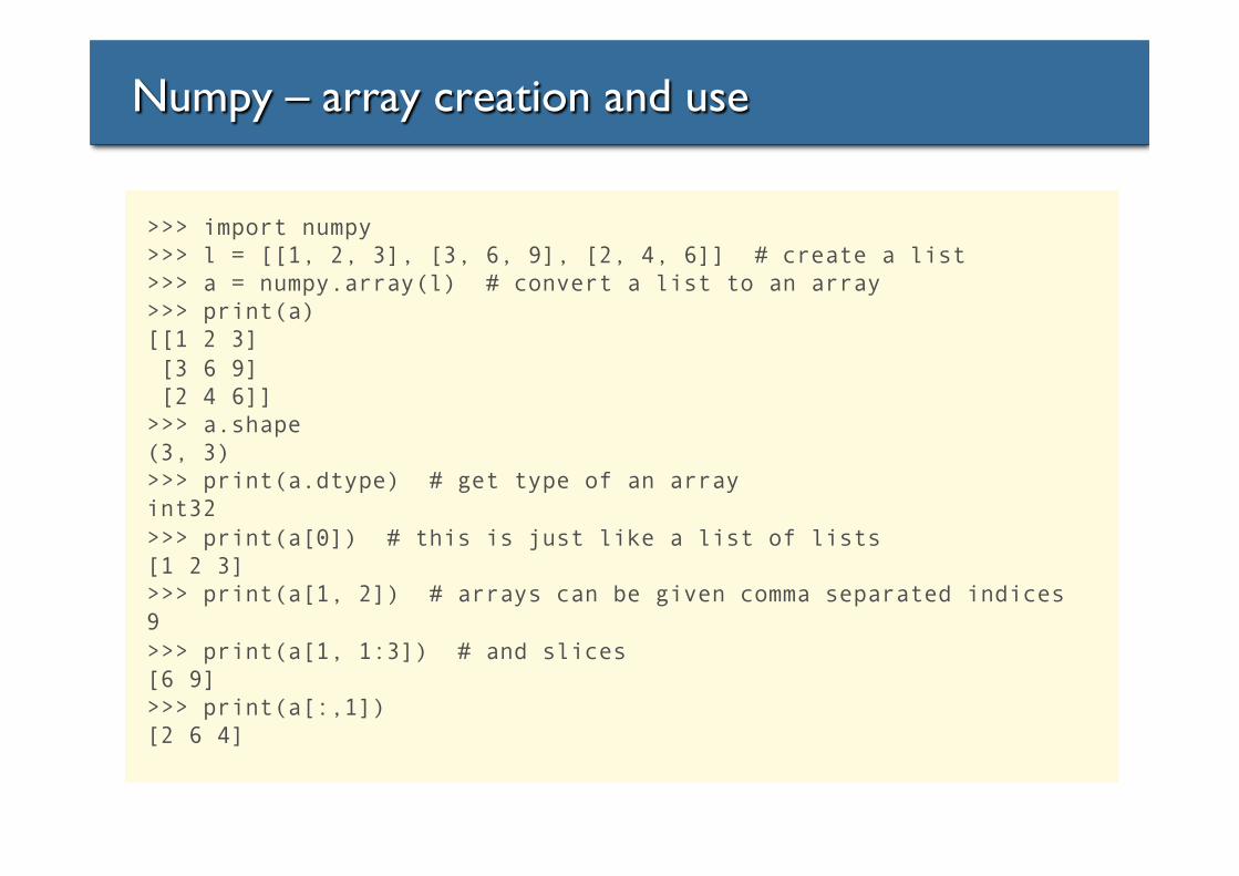
>>> import numpy >>> l = [[1, 2, 3], [3, 6, 9], [2, 4, 6]] # create a list >>> a = numpy.array(l) # convert a list to an array >>> print(a) [[1 2 3] [3 6 9] [2 4 6]] >>> a.shape (3, 3) >>> print(a.dtype) # get type of an array int32 >>> print(a[0]) # this is just like a list of lists [1 2 3] >>> print(a[1, 2]) # arrays can be given comma separated indices 9 >>> print(a[1, 1:3]) # and slices [6 9] >>> print(a[:,1]) [2 6 4]
Numpy – array creation and use
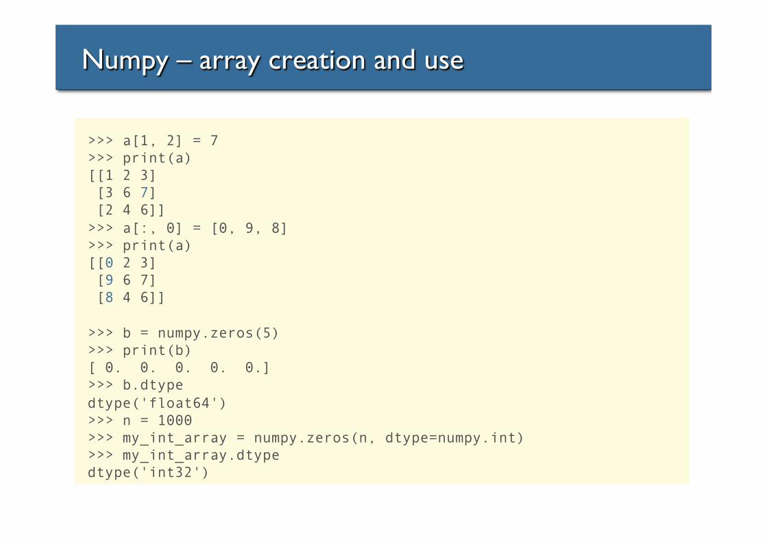
>>> a[1, 2] = 7 >>> print(a) [[1 2 3] [3 6 7] [2 4 6]] >>> a[:, 0] = [0, 9, 8] >>> print(a) [[0 2 3] [9 6 7] [8 4 6]] >>> b = numpy.zeros(5) >>> print(b) [ 0. 0. 0. 0. 0.] >>> b.dtype dtype('float64') >>> n = 1000 >>> my_int_array = numpy.zeros(n, dtype=numpy.int) >>> my_int_array.dtype dtype('int32')
Numpy – array creation and use
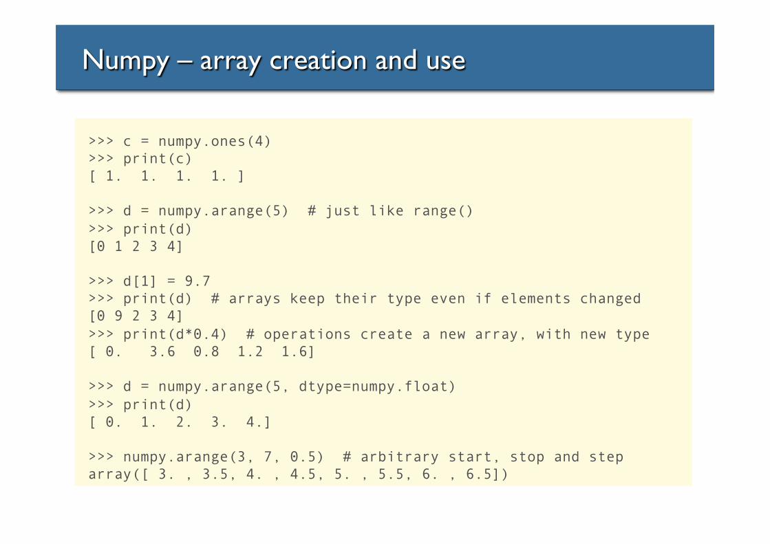
>>> c = numpy.ones(4) >>> print(c) [ 1. 1. 1. 1. ] >>> d = numpy.arange(5) # just like range() >>> print(d) [0 1 2 3 4] >>> d[1] = 9.7 >>> print(d) # arrays keep their type even if elements changed [0 9 2 3 4] >>> print(d*0.4) # operations create a new array, with new type [ 0. 3.6 0.8 1.2 1.6] >>> d = numpy.arange(5, dtype=numpy.float) >>> print(d) [ 0. 1. 2. 3. 4.] >>> numpy.arange(3, 7, 0.5) # arbitrary start, stop and step array([ 3. , 3.5, 4. , 4.5, 5. , 5.5, 6. , 6.5])

Numpy – array creation and use
>>> a = numpy.arange(4.0) >>> b = a * 23.4 >>> c = b/(a+1) >>> c += 10 >>> print c [ 10. 21.7 25.6 27.55] >>> arr = numpy.arange(100, 200) >>> select = [5, 25, 50, 75, -5] >>> print(arr[select]) # can use integer lists as indices [105, 125, 150, 175, 195] >>> arr = numpy.arange(10, 20) >>> div_by_3 = arr%3 == 0 # comparison produces boolean array >>> print(div_by_3) [ False False True False False True False False True False] >>> print(arr[div_by_3]) # can use boolean lists as indices [12 15 18]
Numpy – array creation and use
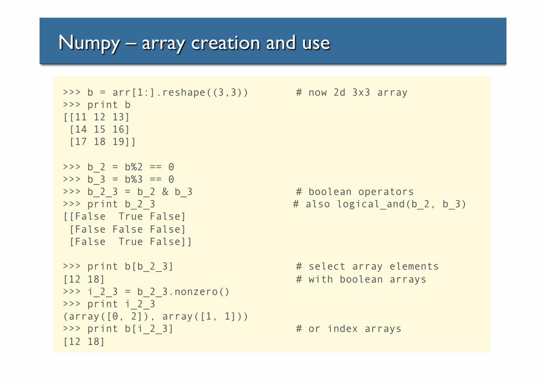
>>> b = arr[1:].reshape((3,3)) # now 2d 3x3 array >>> print b [[11 12 13] [14 15 16] [17 18 19]] >>> b_2 = b%2 == 0 >>> b_3 = b%3 == 0 >>> b_2_3 = b_2 & b_3 # boolean operators >>> print b_2_3 # also logical_and(b_2, b_3) [[False True False] [False False False] [False True False]] >>> print b[b_2_3] # select array elements [12 18] # with boolean arrays >>> i_2_3 = b_2_3.nonzero() >>> print i_2_3 (array([0, 2]), array([1, 1])) >>> print b[i_2_3] # or index arrays [12 18]
Numpy – array methods
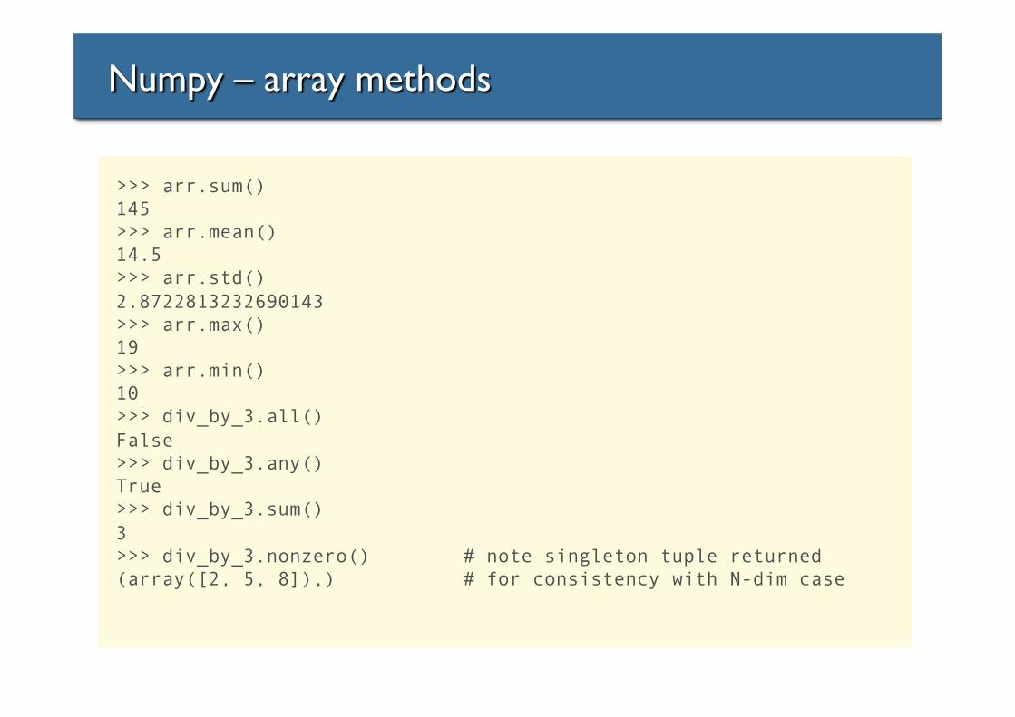
>>> arr.sum() 145 >>> arr.mean() 14.5 >>> arr.std() 2.8722813232690143 >>> arr.max() 19 >>> arr.min() 10 >>> div_by_3.all() False >>> div_by_3.any() True >>> div_by_3.sum() 3 >>> div_by_3.nonzero() # note singleton tuple returned (array([2, 5, 8]),) # for consistency with N-dim case
Numpy – array methods – sorting
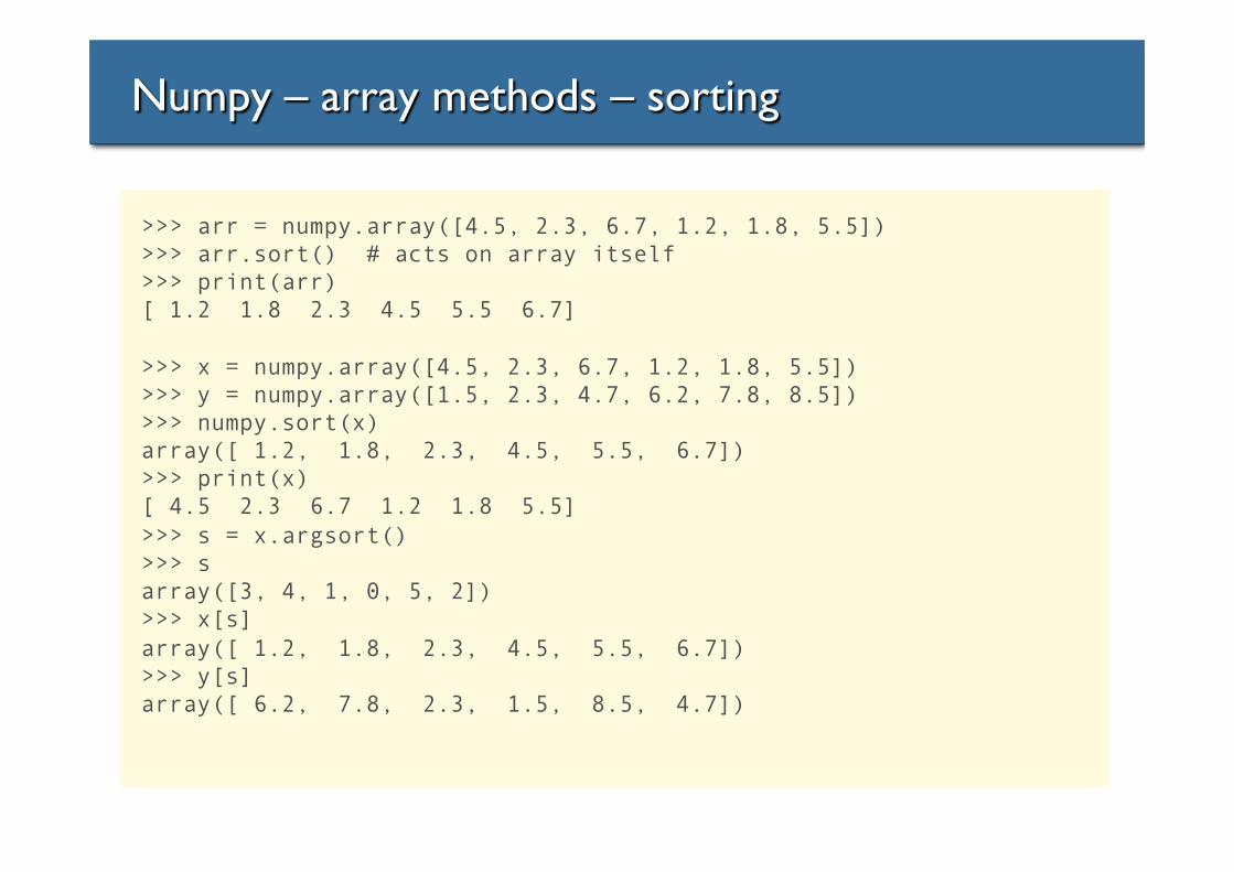
>>> arr = numpy.array([4.5, 2.3, 6.7, 1.2, 1.8, 5.5]) >>> arr.sort() # acts on array itself >>> print(arr) [ 1.2 1.8 2.3 4.5 5.5 6.7] >>> x = numpy.array([4.5, 2.3, 6.7, 1.2, 1.8, 5.5]) >>> y = numpy.array([1.5, 2.3, 4.7, 6.2, 7.8, 8.5]) >>> numpy.sort(x) array([ 1.2, 1.8, 2.3, 4.5, 5.5, 6.7]) >>> print(x) [ 4.5 2.3 6.7 1.2 1.8 5.5] >>> s = x.argsort() >>> s array([3, 4, 1, 0, 5, 2]) >>> x[s] array([ 1.2, 1.8, 2.3, 4.5, 5.5, 6.7]) >>> y[s] array([ 6.2, 7.8, 2.3, 1.5, 8.5, 4.7])
Numpy – array functions
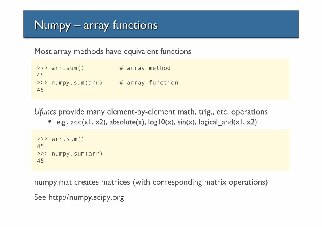
Most array methods have equivalent functions
Ufuncs provide many element-by-element math, trig., etc. operations• e.g., add(x1, x2), absolute(x), log10(x), sin(x), logical_and(x1, x2)
numpy.mat creates matrices (with corresponding matrix operations)
See http://numpy.scipy.org
>>> arr.sum() # array method 45 >>> numpy.sum(arr) # array function 45
>>> arr.sum() 45 >>> numpy.sum(arr) 45
Numpy – array functions
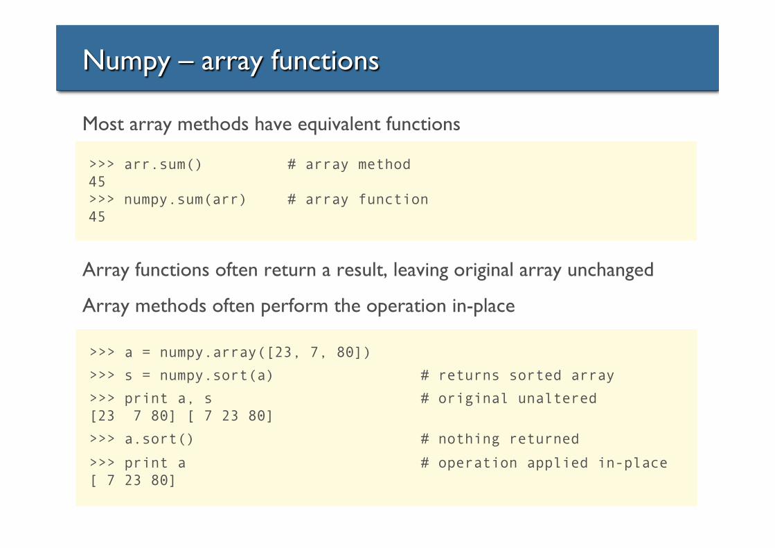
Most array methods have equivalent functions
Array functions often return a result, leaving original array unchanged
Array methods often perform the operation in-place
>>> a = numpy.array([23, 7, 80])
>>> s = numpy.sort(a) # returns sorted array
>>> print a, s # original unaltered [23 7 80] [ 7 23 80]
>>> a.sort() # nothing returned
>>> print a # operation applied in-place [ 7 23 80]
>>> arr.sum() # array method 45 >>> numpy.sum(arr) # array function 45
Numpy – array functions
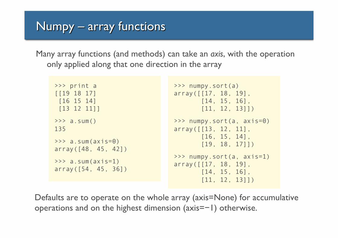
Many array functions (and methods) can take an axis, with the operation only applied along that one direction in the array
>>> print a [[19 18 17] [16 15 14] [13 12 11]]
>>> a.sum() 135
>>> a.sum(axis=0) array([48, 45, 42])
>>> a.sum(axis=1) array([54, 45, 36])
>>> numpy.sort(a) array([[17, 18, 19], [14, 15, 16], [11, 12, 13]])
>>> numpy.sort(a, axis=0) array([[13, 12, 11], [16, 15, 14], [19, 18, 17]])
>>> numpy.sort(a, axis=1) array([[17, 18, 19], [14, 15, 16], [11, 12, 13]])
Defaults are to operate on the whole array (axis=None) for accumulative operations and on the highest dimension (axis=−1) otherwise.

Numpy – random numbers
High quality (pseudo-) random number generator with many common distributions
>>> numpy.random.seed(12345) # or default seed taken from clock >>> numpy.random.uniform() 0.9296160928171479
>>> numpy.random.uniform(-1, 1, 3) array([-0.36724889, -0.63216238, -0.59087944])
>>> r = numpy.random.normal(loc=3.0, scale=1.3, size=100) >>> r.mean(), r.std() (3.1664506480570371, 1.2754634208344433)
>>> p = numpy.random.poisson(123, size=(1024,1024)) >>> p.shape (1024, 1024) >>> p.mean(), p.std()**2 (123.02306461334229, 122.99512022056578)
Numpy – recarray
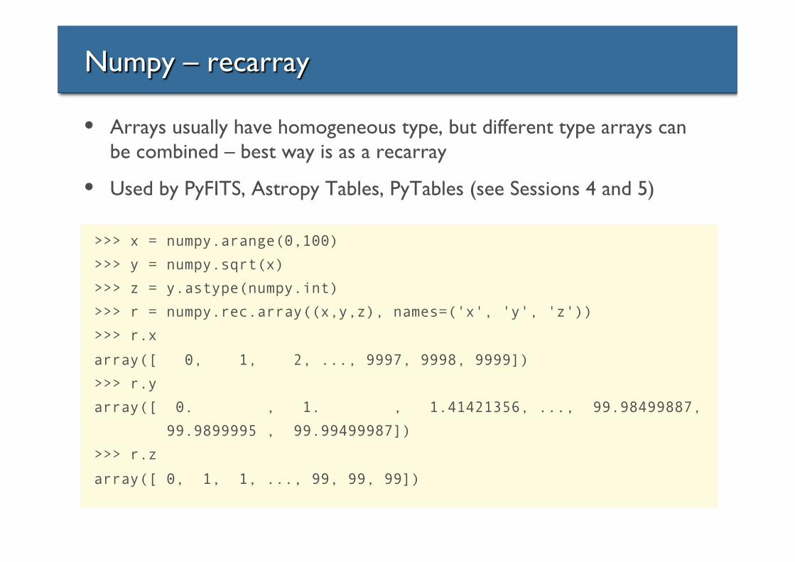
• Arrays usually have homogeneous type, but different type arrays can be combined – best way is as a recarray
• Used by PyFITS, Astropy Tables, PyTables (see Sessions 4 and 5)
>>> x = numpy.arange(0,100)
>>> y = numpy.sqrt(x)
>>> z = y.astype(numpy.int)
>>> r = numpy.rec.array((x,y,z), names=('x', 'y', 'z'))
>>> r.x
array([ 0, 1, 2, ..., 9997, 9998, 9999])
>>> r.y
array([ 0. , 1. , 1.41421356, ..., 99.98499887,
99.9899995 , 99.99499987])
>>> r.z
array([ 0, 1, 1, ..., 99, 99, 99])
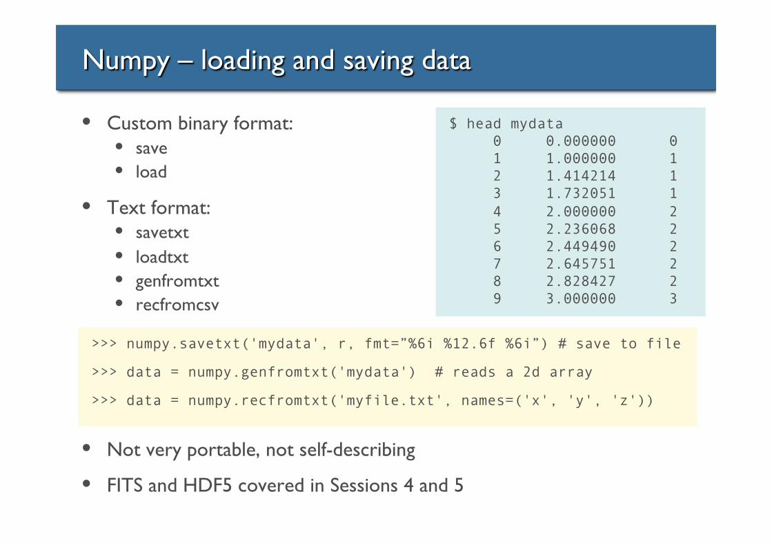
Numpy – loading and saving data
• Custom binary format:• save• load
• Text format:• savetxt• loadtxt• genfromtxt• recfromcsv
• Not very portable, not self-describing
• FITS and HDF5 covered in Sessions 4 and 5
>>> numpy.savetxt('mydata', r, fmt=”%6i %12.6f %6i”) # save to file
>>> data = numpy.genfromtxt('mydata') # reads a 2d array
>>> data = numpy.recfromtxt('myfile.txt', names=('x', 'y', 'z'))
$ head mydata 0 0.000000 0 1 1.000000 1 2 1.414214 1 3 1.732051 1 4 2.000000 2 5 2.236068 2 6 2.449490 2 7 2.645751 2 8 2.828427 2 9 3.000000 3

Numpy – using arrays wisely
• Array operations are implemented in C or Fortran
• Optimised algorithms - i.e. fast!
• Python loops (i.e. for i in a:…) are much slower
• Prefer array operations over loops, especially when speed important
• Also produces shorter code, often much more readable
• If you're working with large datasets, watch out for swapping…
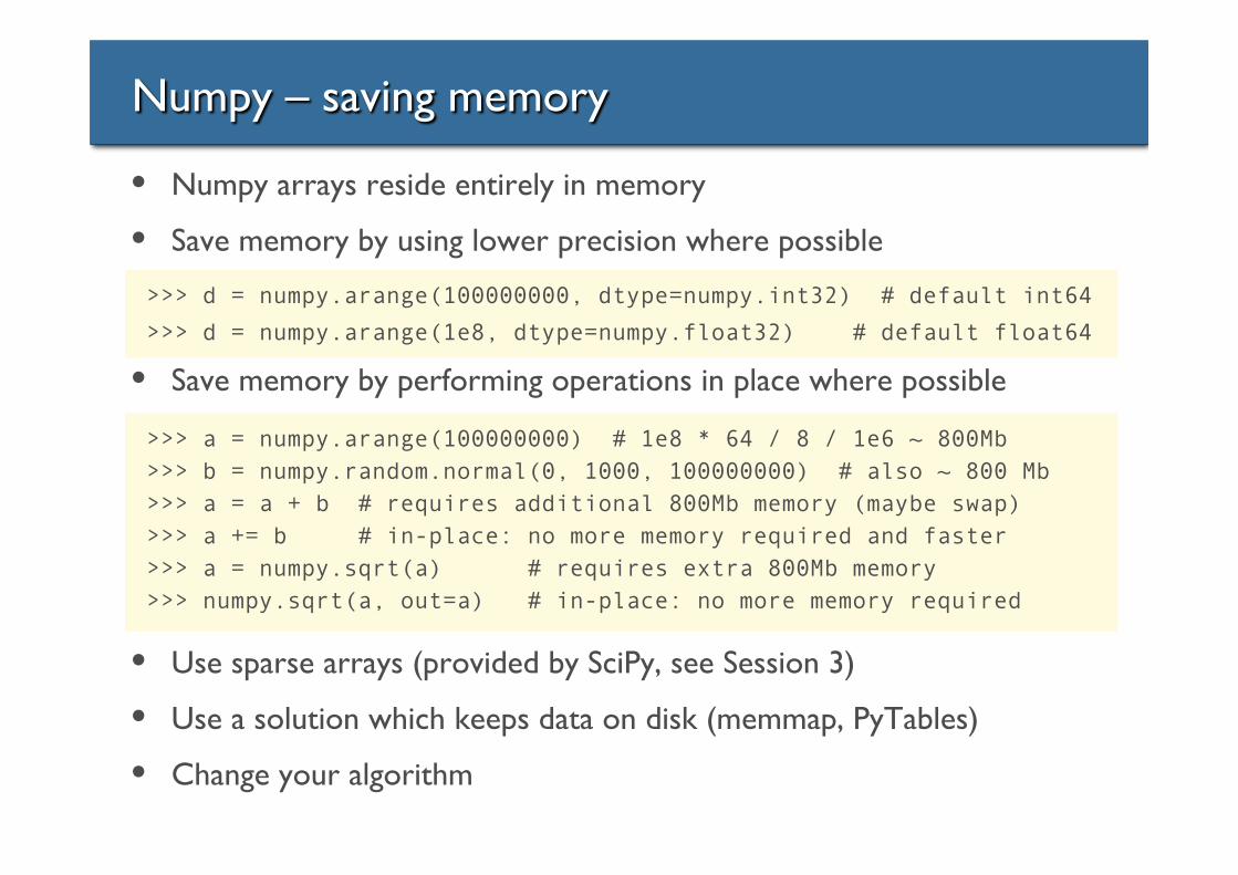
Numpy – saving memory
• Numpy arrays reside entirely in memory
• Save memory by using lower precision where possible
• Save memory by performing operations in place where possible
• Use sparse arrays (provided by SciPy, see Session 3)
• Use a solution which keeps data on disk (memmap, PyTables)
• Change your algorithm
>>> a = numpy.arange(100000000) # 1e8 * 64 / 8 / 1e6 ~ 800Mb >>> b = numpy.random.normal(0, 1000, 100000000) # also ~ 800 Mb >>> a = a + b # requires additional 800Mb memory (maybe swap) >>> a += b # in-place: no more memory required and faster >>> a = numpy.sqrt(a) # requires extra 800Mb memory >>> numpy.sqrt(a, out=a) # in-place: no more memory required
>>> d = numpy.arange(100000000, dtype=numpy.int32) # default int64
>>> d = numpy.arange(1e8, dtype=numpy.float32) # default float64
An explanation
[link]
Plotting – matplotlib
• User friendly, but powerful, plotting capabilities for python
• http://matplotlib.org/
• Once installed, to use type:
• Settings can be customised by editing ~/.matplotlib/matplotlibrc• Set backend and default font, colours, layout, etc.
• Helpful website• many examples
>>> import pylab # handy for interactive use >>> import matplotlib.pyplot as plt # better for in scripts
>>> pyplot.ion() # turn on interactive mode!
Plotting – matplotlib
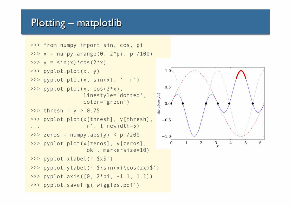
>>> from numpy import sin, cos, pi
>>> x = numpy.arange(0, 2*pi, pi/100)
>>> y = sin(x)*cos(2*x)
>>> pyplot.plot(x, y)
>>> pyplot.plot(x, sin(x), '--r')
>>> pyplot.plot(x, cos(2*x), linestyle='dotted', color='green')
>>> thresh = y > 0.75
>>> pyplot.plot(x[thresh], y[thresh], ... 'r', linewidth=5)
>>> zeros = numpy.abs(y) < pi/200
>>> pyplot.plot(x[zeros], y[zeros], 'ok', markersize=10)
>>> pyplot.xlabel(r'$x$')
>>> pyplot.ylabel(r'$\sin(x)\cos(2x)$')
>>> pyplot.axis([0, 2*pi, -1.1, 1.1])
>>> pyplot.savefig('wiggles.pdf')

Plotting – matplotlib
>>> fig = pyplot.figure(1)
>>> ax = fig.axes[0]
>>> ax.xaxis.labelpad = 10
>>> pyplot.draw()
>>> l = ax.lines[2]
>>> l.set_linewidth(3)
>>> pyplot.draw()
>>> ax.xaxis.set_ticks((0, pi/2, pi, 3*pi/2, 2*pi))
>>> pyplot.draw()
>>> ax.xaxis.set_ticklabels(('0', r'$\frac{1}{2}\pi$', r'$\pi$',
r'$\frac{3}{2}\pi$', r'$2\pi$'))
>>> pyplot.draw()
>>> pyplot.subplots_adjust(bottom=0.25)
• Plots can be altered in an object oriented manner
For example,
Shorthand to get current axes >>> ax = pyplot.gca()
Plotting – matplotlib
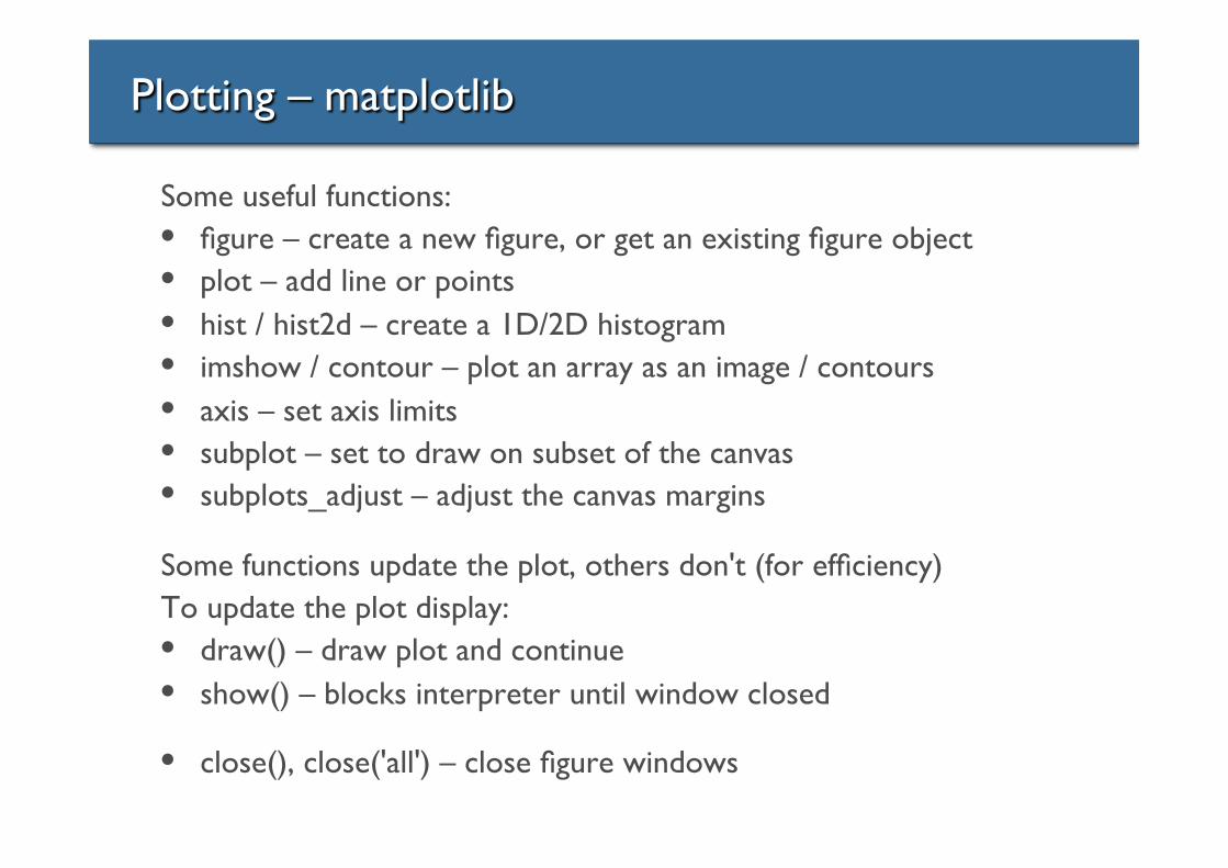
Some useful functions:• figure – create a new figure, or get an existing figure object• plot – add line or points• hist / hist2d – create a 1D/2D histogram• imshow / contour – plot an array as an image / contours• axis – set axis limits• subplot – set to draw on subset of the canvas• subplots_adjust – adjust the canvas margins
Some functions update the plot, others don't (for efficiency)To update the plot display:• draw() – draw plot and continue• show() – blocks interpreter until window closed
• close(), close('all') – close figure windows
Matplotlib/Ipython notebook scatter plot example
[link to online notebook]

Plotting – interactive notebook plots
• There are some new tools for producing interactive plots in a web browser (and hence in IPython notebooks)
• Mpld3• http://mpld3.github.io/
• Bokeh• http://bokeh.pydata.org/
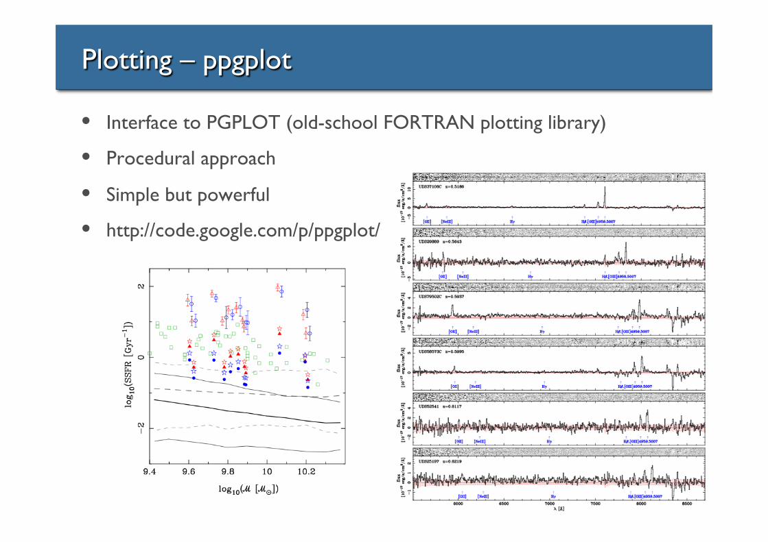
Plotting – ppgplot
• Interface to PGPLOT (old-school FORTRAN plotting library)
• Procedural approach
• Simple but powerful
• http://code.google.com/p/ppgplot/
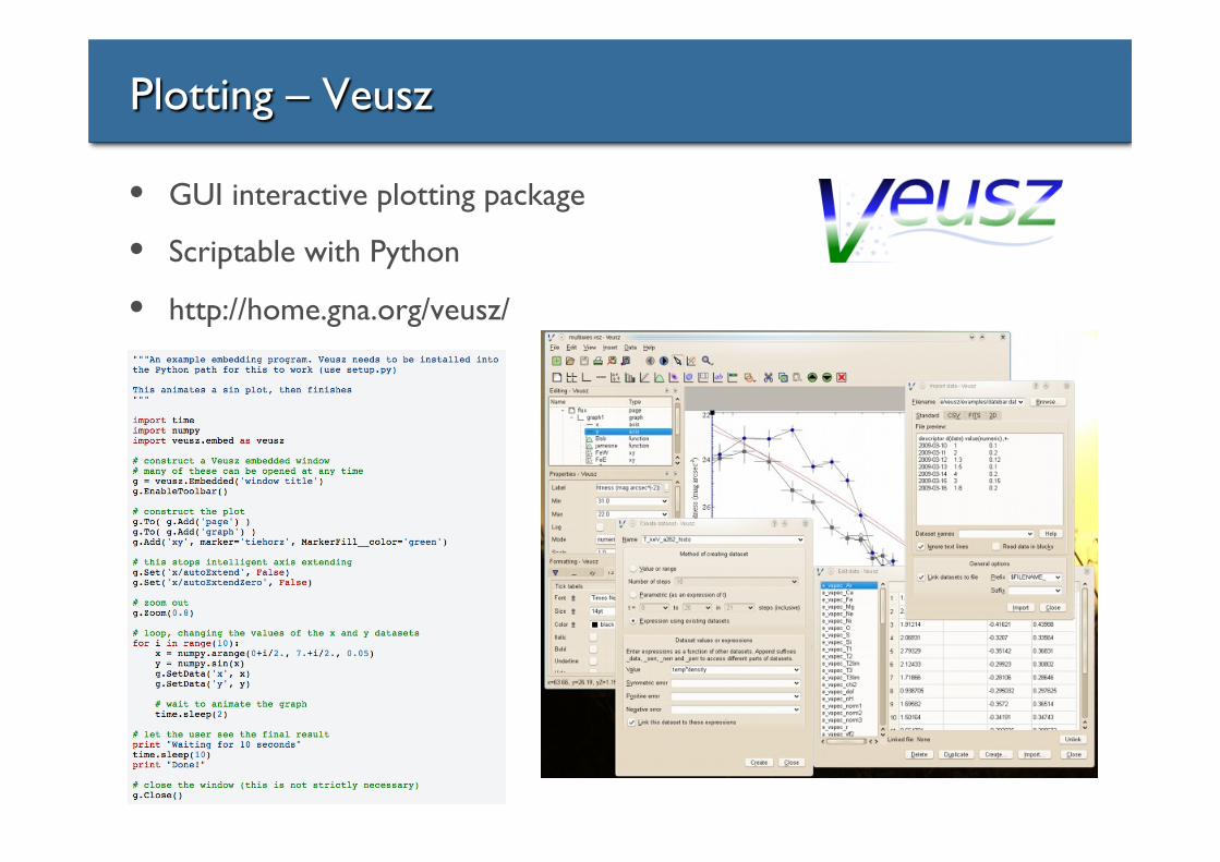
Plotting – Veusz
• GUI interactive plotting package
• Scriptable with Python
• http://home.gna.org/veusz/
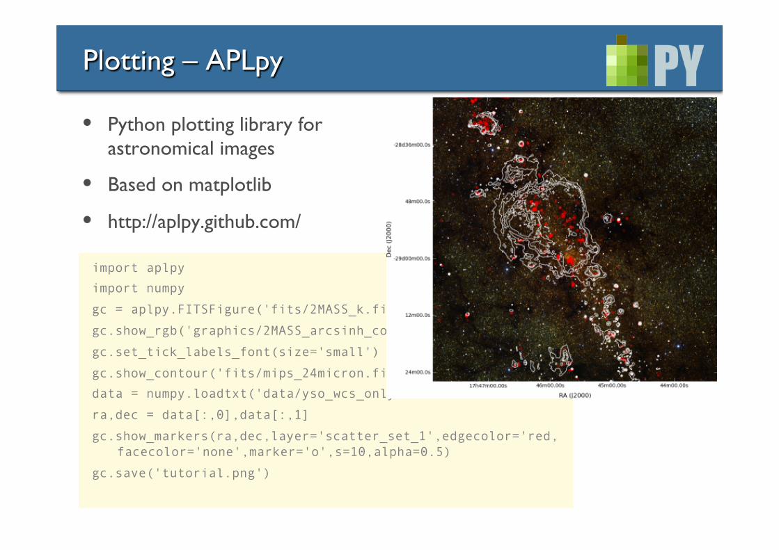
Plotting – APLpy
• Python plotting library for astronomical images
• Based on matplotlib
• http://aplpy.github.com/
import aplpy
import numpy
gc = aplpy.FITSFigure('fits/2MASS_k.fits',figsize=(10,9)
gc.show_rgb('graphics/2MASS_arcsinh_color.png')
gc.set_tick_labels_font(size='small')
gc.show_contour('fits/mips_24micron.fits',colors='white')
data = numpy.loadtxt('data/yso_wcs_only.txt'
ra,dec = data[:,0],data[:,1]
gc.show_markers(ra,dec,layer='scatter_set_1',edgecolor='red, facecolor='none',marker='o',s=10,alpha=0.5)
gc.save('tutorial.png')
Coursework
• A Python program relevant to your research• put course material into practice• opportunity to become familiar with Python• get feedback on your coding • requirement to qualify for credits
• Your program should…• be written as an importable module (.py file)• do something meaningful: analyse real data or perform a simulation• use at least two user functions• use at least one of the modules introduced in Sessions 3 – 5• produce at least one informative plot • comprise >~ 50 lines of actual code (excluding comments and imports)
Coursework
• Submit as source code (.py file) and pdf/png files of the output plot(s)• Ideally as GitHub repo.
• Visit here: https://classroom.github.com/assignment-invitations/b410e0094b06d7be5c8054797a9b924b
• (link also on the course webpage)• I will also accept submissions via email ([email protected])
• Three stages:• by 23 October
• README describing what you intend your code to do• Rough outline of the code (classes, functions, snippets, comments, pseudocode)• Feedback in a week
• by 6 November• Roughly working version of your code, although may be incomplete, have bugs,
although try to make it reasonable and easy to understand!• Feedback in a week
• by 27 November• Full working version of your code (doesn’t have to be amazing – just work!)• Feedback and confirmation of pass by end of term
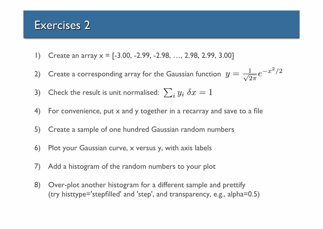
Exercises 2
1) Create an array x = [-3.00, -2.99, -2.98, …, 2.98, 2.99, 3.00]
2) Create a corresponding array for the Gaussian function
3) Check the result is unit normalised:
4) For convenience, put x and y together in a recarray and save to a file
5) Create a sample of one hundred Gaussian random numbers
6) Plot your Gaussian curve, x versus y, with axis labels
7) Add a histogram of the random numbers to your plot
8) Over-plot another histogram for a different sample and prettify (try histtype='stepfilled' and 'step', and transparency, e.g., alpha=0.5)
Pi yi �x = 1
y = 1p2⇡
e�x
2/2