Services Trade Costs: Tariff equivalents of services trade...

Services Trade Costs: Tariff equivalents of services trade restrictions using gravity estimation∗+

July 27, 2016

Preliminary and incomplete Please do not cite

Abstract

Services trade restrictions can impose significant costs on importers and exporters of services. This paper presents evidence on ad valorem tariff equivalents of the OECD Services Trade Restrictiveness Index (STRI) for cross-border services trade. Importantly, these tariff equivalents do not rise linearly with a country’s STRI score in many sectors. In addition, detailed information on the classification of measures in the STRI database is used to show that different types of regulatory policies contribute unequally to services trade costs for cross-border trade, even though these policies account for identical STRI scores.

Sebastian Benz Organisation for Economic Co-Operation and Development

2, rue André Pascal 75775 Paris Cedex 16, France

Tel: +33 1 85 55 68 21 [email protected]

∗ The author is writing in a strictly personal capacity. The views expressed are his only, and do not reflect in any

way those of the OECD Secretariat or the member countries of the OECD. + This paper has benefitted from helpful comments and discussions with Ken Ash, Charles Cadestin, John

Drummond, Frederic Gonzales, Andrea Marin Odio, Hildegunn Nordås, Dorothée Rouzet and Francesca Spinelli.

1. Introduction

Services trade restrictions can impose significant costs on importers and exporters of services. This report presents detailed evidence on the importance of the OECD Services Trade Restrictiveness Index (STRI) for the cost of cross-border services trade.1 The STRI represents the state of regulatory restrictions in 19 different services sectors and 42 countries2 on a scale from 0 to 1.

This paper presents estimated ad valorem trade cost equivalents of services trade restrictions for cross-border trade in services as well as estimated trade effects, which indicate the resulting growth in trade volumes from the reduction of services trade restrictions. While these two concepts are closely linked, both have their particular advantages. Trade cost equivalents provide direct information on the size of services trade restrictions, but they rely on estimates of import demand elasticities taken from the literature. Since it is not possible to determine an exact value for the import demand elasticity, I report results for different values within a range of plausible values. Trade effects provide information on the welfare effect of trade liberalisation, because changes in welfare are larger if consumers are actually willing to substitute foreign products or services for domestic products or services after a reduction of trade costs.3 These trade effects can be calculated directly from the coefficients of gravity regressions, without having to rely on any additional information. Both, the derivation of trade cost equivalents as well as the prediction of the trade effect of services trade liberalisation, are important components of ex ante policy evaluation. Nevertheless, two aspects of how services trade restrictions affect consumer welfare are not captured by these measures:

• GATS Mode 3 of services trade (commercial presence) is not included in trade in services statistics from the balance of payments. Therefore, it is not possible to account for this Mode of services trade in the present report. In situations where the STRI has no significant effect on the cost of cross-border trade in services, it might actually represent substantial costs for the provision of services trade via Mode 3. The relationship of the STRI and services trade via Mode 3 is not part of this study but will be explored in the future, primarily by exploiting information on foreign affiliate sales from firm-level data.4

• Several measures in the STRI capture more than only restrictions to services trade. For example, restrictions in policy area 4, barriers to competition, do not only protect dominant domestic firms from foreign competitors, but also from domestic competitors. In such a situation, trade flows are not sufficient as proxy for consumer welfare. This shows the importance of analysing the relationship between the STRI and the level of competition in an economy.

With these caveats in mind, this paper shows that the ad valorem trade cost equivalent of services trade restrictions can be very high in some sectors, but the estimates depend strongly on the assumed import demand elasticity. Subsequently, it reveals that different types of regulatory policies contribute unequally to services trade costs, even though these policies account for identical STRI scores. Moreover, it describes how the impact of services trade liberalisation on trade flows depends on observable country characteristics, such as GDP, GDP per capita and geographic size. The report is organised as follows: Section 2 summarises the existing literature on services trade costs; section 3 presents the data used for the estimations; section 4 provides an overview on the methodology; section

1 The STRI database and indices are available at http://oe.cd/stri. 2 Country coverage includes all 34 OECD Members plus Brazil, China, Colombia, India, Indonesia, Latvia,

Russia and South Africa. 3 Accordingly, the value of trade flows relative to GDP is a proxy for the level of consumer welfare in a large

group of economic models, see Arkolakis et al. (2012). 4 Services trade via Mode 3 is very important. For example, foreign affiliate sales of services accounted for 68%

of US cross-border exports of services and foreign affiliate sales in 2012 (Christen and Francois, 2015).

5 shows the estimated trade cost equivalents of the aggregate STRI and its decomposition into different groups; section 6 concludes.

2. Literature Review

Several existing publications present estimates on trade costs for services. Most of these studies do not use information on restrictions to services trade. Instead, they estimate the size of aggregate services trade cost based on a comparison of a country’s services trade volume relative to services trade in a benchmark country or relative to domestic consumption of services. The two strategies can provide evidence on the aggregate trade costs for services, but neither of them is able to identify whether services trade costs are due to political or natural trade barriers.

Fontagné et al. (2011) estimates trade costs for 9 services sectors based on services trade data from the Global Trade Analysis Project (GTAP) data base. Estimates for average tariff equivalents range between 20% for transport services and 65% for construction services. Barriers in the most restrictive country represent trade costs between 49% and 160%. These estimates represent trade costs relative to a trade costs in a benchmark country with the highest volume of trade in services, given its observable characteristics. Benchmark countries with low levels of restrictions are Hong Kong, Belgium, Austria, Singapore, Ireland, Mexico and Greece, depending on the sector in question. The authors use an import demand elasticity of 4.6 which indicates that foreign and domestic services are relatively good substitutes. In a subsequent paper, Guillin (2013) estimates tariff equivalents between 28% and 71% using a very similar approach but considering zero trade flows explicitly in a Heckman selection model.

A different approach is used by Miroudot et al. (2013) and Miroudot and Shepherd (2015). Tariff equivalents of total trade costs are not calculated relative to a benchmark country but instead they are based on a country’s volume of trade in services relative to domestic consumption of services. Since this measure implies positive services trade costs even for the most liberal benchmark country, the resulting tariff equivalents are substantially larger for all countries in the sample and on average. The average tariff equivalent for services trade costs is calculated as 155% based on an import demand elasticity of 7. Due to the difference in the elasticity chose, results of the two studies are not directly comparable.5 Since sectors can differ with respect to their services trade costs, some sectors must necessarily be characterised by lower trade costs, while trade costs in other sectors can be substantially higher.

Anderson et al. (2014) use information on services trade of Canadian regions with the United States. They find that all Canadian regions trade significantly less with the US than they trade among each other. Using import demand elasticities between 5 and 9 they estimate that the difference between services trade across the US-Canada border and intra-Canada services trade corresponds to a tariff equivalent between 52% and 111% for exporting services from Canada to the United States. This approach relies on the unique data set of regional services trade in Canada.

Berden et al. (2009) estimate trade cost equivalents of non-tariff measures (NTM) based on a business survey. Survey results are used to construct country-pair-specific NTM barriers. They use a two-step Heckman approach to control for selection into bilateral export relationships. This approach must be usually based on an exclusion restriction: An explanatory variable which has a significant coefficient in the selection equation but does not contribute to the explanation of bilateral trade volumes, once that selection is taken into account (Puhani, 2000). However, the authors do not provide a convincing explanation for the exclusion restriction used in their estimation, which raises questions on the validity of the results.

5 A back of the envelope calculation suggests that the result by Miroudot et al. (2013) correspond to a 316%

average tariff equivalent based on an import demand elasticity of 4.6. This is calculated as (1.55 +1)! !.! − 1.

So far there exists little evidence on the estimation of services trade costs originating from regulatory barriers using constructed indices of services trade restrictiveness. Van der Marel and Shepherd (2013) identify a significantly negative effect of the World Bank STRI on services trade while Nordås and Rouzet (2015) find the same for the OECD STRI. However, these studies do not calculate tariff equivalents of services trade costs. Existing firm-level studies usually do not quantify ad valorem equivalents of services trade barriers but rather characterise the patterns of services trade. Examples thereof can be found in Crozet and Milet (2014), Breinlich and Criscuolo (2011), Ariu and Mion (2012), Walter and Dell’mour (2010) and Kelle and Kleinert (2010).

3. Data

All results in this report are based on STRI scores calculated according to the new STRI methodology (2015 update) but using the regulatory framework of 2014. Since no trade data for 2015 is available yet, the regulatory framework of 2014 is most appropriate for the representation of restrictions to services trade in the regression analysis. In addition to the aggregate STRI scores, further specifications of the regression are based on a decomposition of the STRI into individual groups which represent a more narrowly defined and homogeneous set of services trade restrictions than the aggregate STRI.

Data on the value of services production come from the OECD national accounts data. The classification of production data is more aggregate than the classification of data on trade flows in some cases so that an exact sector correspondence is not always feasible. This reduces sector coverage for this type of analysis slightly compared to an estimation based only on trade data. Services trade flows come from three different data sources: The OECD Trade in Services by Partner Country (TISP) data; the WTO-UNCTAD-ITC trade in services database; and the United Nations Service Trade database, of which TISP is the preferred data source. When no information on the export volume is available, imports reported by the partner country are used to fill the gaps wherever possible.

Trade data is only scarcely available for the year 2014 so far. Hence, all regressions are based on trade flows from 2010 to 2013. Data from before 2010 is not used because the STRI captures the level of services trade restrictions in 2014. Restricting the sample to all available years since 2010 implies a sufficient number of observations while at the same time limiting the time mismatch between the state of regulatory environment and observed trade flows. Unfortunately, no balanced panel of export data is available for any sector. Exporter information is available only for 31 countries out of the 42 STRI countries, while all 42 countries are included as importing countries.

This study analyses six STRI sectors: computer services (CS), construction (CO), courier services (CR), telecommunications (TC), maritime transport (TRmar) and commercial banking (FSbnk). Countries in the sample report an aggregate export volume of 175 billion USD in these six sectors over the four years covered. The mean value of annual bilateral exports is highest in the banking sector, with around 139 million USD. In contrast, exports are relatively low in courier services, construction services, and telecommunication services. Bilateral exports on the sector level are characterised by a relatively high number of zeros. The share of zeros varies between 29% in computer services and 55% in courier services.

Table 1. Characterisation of exports 2010-2013 by sector (in million USD)

Observations Mean Std. Dev. Maximum Share of zeros Construction (CO) 4 961 24 86 1 529 44.02% Computer (CS) 4 510 103 386 7 686 28.51% Courier (CR) 3 895 10 79 3 070 54.63% Telecommunication (TC) 4 346 30 112 1 933 37.37% Maritime transport (TRmar) 2 730 134 454 7 312 31.79% Commercial banking (FSbnk) 4 510 139 686 13 976 30.24%

4. Methodology

The gravity model is the workhorse model for the analysis of international trade flows, not only for trade in goods, but also for services. In this model, bilateral trade flows are explained by observable country characteristics and country-pair characteristics. These characteristics typically include domestic expenditure (usually measured by GDP), bilateral distance, common language, bilateral trade agreements and many more. While this base specification has not lost its relevance, several extensions have been developed which allow for more tightly focussed analysis.

For the application of gravity estimation to services trade restrictions, a major difficulty arises from the multilateral property of the STRI score. Each county’s STRI represents an identical level of services trade restrictions with respect to all partner countries; a country-pair dimension does not exist. However, in the modern gravity regressions introduced by Anderson and van Wincoop (2003) coefficients on country-specific variables cannot be identified because country-level fixed effects are used to control for a country’s unobservable multilateral resistance to trade.

While there are real country-specific variables such as GDP or population, the STRI does not constitute such a real country-specific variable. It is rendered a country-specific variable in a standard gravity equation by assuming that trade with all other countries is affected identically by a country’s services trade restrictions. But what about domestic sales of domestic services suppliers? Due to the nature of the STRI it is not possible to assume that the supply of services from domestic producers to domestic consumers is unaffected by services trade restrictions. However, it is valid to assume that domestic producers are affected differently from foreign producers.

The availability of data on the value of services production in each country allows to construct measures of so-called ‘within-country trade flows’, defined as the value of domestically produced services which are consumed domestically. Technically, these are constructed by subtracting the aggregate value of exports in a sector from the value of production in this sector. This section provides a less-technical and more intuitive description of the estimation strategy based on these ‘trade flows’. More technical information can be found in the following box.

Box 1. Estimation strategy

All regressions are run separately for each sector and are estimated using the poisson pseudo maximum likelihood technique developed introduced by Santos Silva and Tenreyro (2006). The estimation equation for each of these sector-level regressions can be written as

𝑒𝑥𝑝𝑜𝑟𝑡𝑠!"#,! = exp(𝛽!𝑆𝑇𝑅𝐼!,!𝑏𝑜𝑟𝑑𝑒𝑟!" + 𝛽!𝑏𝑜𝑟𝑑𝑒𝑟!" + 𝛾𝑍!" + 𝜂! !+ 𝜇!" + 𝜀!"#),

where i indicates the exporter, j indicates the importer, t indicates the year, k indicates the service sector and exp(.) is an exponential function. The variable exports represents bilateral sector-level exports, including the volume of domestic services which is consumed domestically for country pairs where i=j, border is a binary variable which takes the value of zero when i=j and the value of one otherwise. Z is a vector of bilateral gravity control variables, η is an exporter-year dummy, µ is an importer-year dummy and ε is a normally distributed error term. Finally, STRI is a vector of variables indicating services trade restrictiveness, consisting of linear STRI scores and squared STRI scores. Of interest is β0, a vector of regression coefficients.

To control for trade cost with respect to intra-EEA trade, the interaction of the STRI and a dummy which is equal to 1 if importer and exporter are members of the European Economic Area (EEA) is added as additional elements of this vector. This means that the vector product 𝛽!𝑆𝑇𝑅𝐼!,! can be written as

𝛽!𝑆𝑇𝑅𝐼!,! = 𝛽!"𝑆𝑇𝑅𝐼!,! + 𝛽!"𝑆𝑇𝑅𝐼!,!! + 𝛽!"𝑆𝑇𝑅𝐼!,!𝐸𝐸𝐴!" + 𝛽!"𝑆𝑇𝑅𝐼!,!! 𝐸𝐸𝐴!".

To account for the heterogeneity of the trade effect with respect to observable country characteristics, the vector includes the interaction of the STRI with the natural logarithm of the importers’ GDP, GDP per capita and internal distance. In this case, the vector product from above includes additional terms

𝛽!!𝑆𝑇𝑅𝐼!,!𝑙𝑛𝐺𝐷𝑃!" + 𝛽!!𝑆𝑇𝑅𝐼!,!𝑙𝑛𝐺𝐷𝑃𝑝𝑐!" + 𝛽!!𝑆𝑇𝑅𝐼!,!𝑙𝑛𝑑𝑖𝑠𝑡!" + 𝛽!!𝑆𝑇𝑅𝐼!,!𝐸𝐸𝐴!"𝑙𝑛𝐺𝐷𝑃!" + 𝛽!!𝑆𝑇𝑅𝐼!,!𝐸𝐸𝐴!"𝑙𝑛𝐺𝐷𝑃𝑝𝑐!" + 𝛽!!𝑆𝑇𝑅𝐼!,!𝐸𝐸𝐴!"𝑙𝑛𝑑𝑖𝑠𝑡!" .

Trade effects of an STRI reduction by 0.01 are calculated as

𝛥 = [exp −0.01(𝛽!! + 𝛽!! 2 ∗ 𝑠𝑡𝑟𝑖 − 0.01 + 𝛽!! ∗ 𝑙𝑛𝐺𝐷𝑃 + 𝛽!! ∗ 𝑙𝑛𝐺𝐷𝑃𝑝𝑐 + 𝛽!! ∗ 𝑙𝑛𝑑𝑖𝑠𝑡) − 1]∗ 100,

where 𝛽!" is the coefficient on the linear STRI term, 𝛽!" is the coefficient on the quadratic STRI term and 𝛽!! , 𝛽!! and 𝛽!! represent the coefficients of the STRI with ln GDP, ln GDP per capita, and ln internal distance. The variable stri is the initial level of services trade restrictions for which the trade effect is calculated. The tariff equivalent of the STRI is calculated as

𝜏 = [exp (𝑠𝑡𝑟𝑖!"#! − 𝑠𝑡𝑟𝑖)(𝛽!! + 𝛽!! 𝑠𝑡𝑟𝑖 + 𝑠𝑡𝑟𝑖!"#! )/𝜖 − 1] ∗ 100,

where 𝑠𝑡𝑟𝑖 is the STRI score to which the tariff equivalent corresponds, 𝑠𝑡𝑟𝑖!"#! is the second lowest STRI score in the sample of countries for which trade data is available and ε is the import demand elasticity. As above, 𝛽!" is the coefficient on the linear STRI term, 𝛽!" is the coefficient on the quadratic STRI term. Trade cost equivalents can either be calculated for the aggregate STRI or for different components of the STRI.

Standard errors are clustered on the importer-level, to account for a correlation of regression residuals along this dimension. Such a correlation might be due to the lack of country-pair variation in the STRI. Confidence intervals on the tariff equivalent and trade effect can be obtained by first considering the linear combinations of the linear and square term. In a second step, confidence intervals on these linear combinations are transformed by an exponential transformation similarly to the calculation of the tariff equivalents and the trade effect itself. Using the delta method to account for the nonlinear transformation and obtain standard errors yields relatively similar results.

To include within-country trade flows in a gravity analysis, an otherwise standard gravity equation is augmented by a binary variable indicating international trade, the so-called border dummy, i.e. the variable is zero when the services-producing country is equal to the services-consuming country and one in all other cases.6 If frictions to cross-border trade in services exist the coefficient on the border dummy should be significant and negative. The impact of services trade restrictions on trade flows is identified from the interaction of the STRI score with the border dummy. The coefficient on this interaction indicates whether services trade restrictions - as measured by the STRI – affect the volume of trade across borders relative to domestic consumption of domestic services. A negative coefficient implies that countries with a higher STRI score trade less with other countries than countries with a lower STRI score. In other words, more restrictive countries face a higher tariff equivalent for the imports of services.

Since the coefficient on the STRI is identified from data with an exporter-dimension, importer-dimension and year-dimension, exporter-year and importer-year fixed effects can be included in the regression to account for multilateral resistance. These fixed effects also absorb all other country specific variables.7 This advantage comes at the cost of slightly smaller sector coverage, since data quality on the value of production is not sufficiently good for all sectors covered by the STRI.

As mentioned above, the STRI represents barriers on an MFN basis and does not capture more liberal regulation from preferential agreements so that the volume of services trade within the EU may lead to biased results for the impact of the STRI on trade flows in these countries. In order to deal with this problem two additional variables are included. The first is a dummy variable which indicates trade flows within the European Economic Area (EEA) and the second is calculated as the interaction of the STRI-border interaction used in the respective specification with the EEA dummy. The coefficient on this variable captures trade flows between two EEA countries, while the regular STRI variable is only identified from the remaining variation of trade flows which include at least one non-EEA member.

All regressions control for the standard gravity variables, such as the natural logarithm of bilateral distance, contiguity, common language, colonial history, bilateral time differences, bilateral free trade agreements covering services, etc. Moreover, all regressions control for measures of regulatory heterogeneity of the STRI, as calculated in Nordås (2016).8 Since these are all bilateral variables, they can be included as control variables without additional interactions. All these variables take values of zero for within-country trade flows, so that their coefficients only represent trade costs for international trade, while the difference between trade costs for international trade and within-country trade is captured by the border dummy.

Two additional control variables are inserted as proxies for language skills, using information on each country’s number of student studying abroad and the number of students studying abroad in an

6 The importance of within-country trade flows follows directly from the theoretical gravity equation in

Anderson and van Wincoop (2003), where the resulting gravity equation 𝑋!" = !!!!!

!!"!!!!

!!! also

holds for i=j and the entire system of equations is homogeneous of degree zero in the vector of trade costs tij, so that only the effect of relative changes in trade costs (for example costs for international trade relative to domestic trade) can be identified. See Chen (2004), Evans (2003) or Wei (1996) for early research based on this strategy.

7 Due to these methodological improvements, results in this paper can be considered somewhat more reliable than those from previous evidence on the impact of services trade restrictiveness on trade flows by Nordås and Rouzet (2015).

8 The measure of regulatory heterogeneity provides information on the dissimilarity of regulation in two countries according to the STRI. The measure is equal to one for a country pair, if the two countries obtain different scores for each measure in the STRI, while it is equal to zero if two countries obtain identical scores for all measures.

English-speaking country relative to the size of the population.9 Language skills can be an important determinant for the volume of cross-border trade in services which is not driven by the regulatory regime in a sector, but by the quality of a country’s education system. Moreover, in four of the six sectors I control for the share of household with internet access. This variable captures the access to e-commerce which can be an important determinant of services trade flows, for example in courier services. This variable is not included for the regressions in the computer services and telecommunications sector, since the variable is potentially determined by the STRI in these sectors. This means that the effect of the STRI on trade flows could no longer be identified from the STRI variable itself, if the broadband access variable was included. Since these variables do only contain variation on the country-level they are interacted with the border dummy to be included in the regression.

Linear and quadratic terms of the STRI are included in most regressions to identify the potentially nonlinear effect of services trade restrictions on trade costs. This is a relatively simple and straightforward approach to account for the fact that the effect of additional trade barriers on trade costs may depend on the initial level of restrictiveness in a country. The coefficient on the quadratic term should be significantly different from zero in this case. Quadratic terms are not included, if they do not improve the fit of the estimation equation.

Since all coefficients are identified from variation across countries, not from variation over time, the derived trade costs and trade effects must be understood as long run potential of trade liberalisation. This implies that trade costs will not fall immediately after a liberalisation of services trade. There exists some evidence that trade liberalisation takes quite some time before coming into economic effect entirely, even though most evidence is based on data of trade in goods. For example, Baier and Bergstrand (2007) find a 10 year “phase-in” period for the effect of free trade agreements on trade growth. Such a time horizon also seems plausible for the required time until a regulatory reform fully translates into lower trade costs and additional trade in services.

One reason for this long “phase-in” period is that services providers need to adjust to the new regulatory environment. For example, it is likely that services trade providers will invest more in services trade capacities, services trade infrastructure or specific knowledge about foreign markets when the regulation is more liberal towards trade in services. If such investment reduces the cost of cross-border trade, this effect is also captured in the estimated coefficients, since the effect of this investment on trade costs cannot be separated from the tariff equivalent of the STRI in a cross-country analysis. This means that part of the tariff equivalent of the STRI may represent the lack of investment which has not yet taken place due to a restrictive regulatory environment which does not promote services trade.

All results represent the outcomes of independent regressions on the sector-level. This approach allows for a heterogeneous impact of services trade restrictions on trade flows across sectors. The additional flexibility makes this approach superior to a joint regression based on trade data from all services sectors, but comes at the cost of fewer observations per regression, which may increase the standard errors of the estimation coefficients. Estimates are based on the poisson pseudo maximum likelihood estimator, as suggested by Santos Silva and Tenreyro (2006). With this strategy, zero trade flows can explicitly be accounted for in the regression.

5. Trade cost equivalents of the STRI

The link between observed differences in trade flows and implicit trade cost equivalents is established via import demand elasticities. These import demand elasticities are not known and there exists a large literature trying to estimate their values. Most approaches focus on estimates of the elasticity of

9 For countries with English as official language this variable contains the value of Luxembourg, which is the

country with the highest ratio of students studying abroad in an English speaking country relative to the size of its population in my sample of countries in which English is not official language.

substitution σ so that the import demand elasticity is given by 𝜀 = 1 − 𝜎 and relatively more evidence exists for goods than services.

In particular for goods there exists some evidence that the elasticity of substitution has decreased over time. Broda and Weinstein (2006) report an average σ of 6.8 in the period between 1972 and 1988 based on 246 different categories of products. At the same level of product aggregation they find a mean elasticity of 4.0 between 1990 and 2001. Due to the existence of outliers with very large values, sample medians are much smaller than arithmetic averages. In the same study, Broda and Weinstein (2006) find a median of 2.5 between 1972 and 1988 and a median of 2.2 between 1990 and 2001. Using a more disaggregate product classification usually leads to higher estimates for the elasticity of substitution. However, that would be inconsistent with the estimation of trade costs for services on the sector level, for which only relatively aggregate trade data are available.

More recently, Breinlich (2010) estimates the elasticity of substitution for 14 different services categories. His preferred specifications provide results in the range between 1.13 and 2.49, significantly smaller than for goods. He acknowledges the fact that some of the difference between the elasticity of substitution for goods and services might be due to an aggregation bias when services trade flows are reported at a more aggregate level than goods trade. However, he also argues that “services are by their very nature highly differentiated, tailored to individual customers and thus not easily substitutable” (Breinlich, 2010).

Given this evidence, values between -1.5 and -5 can be considered as reasonable estimates for the import demand elasticity. This is at the lower end of what has previously been used in the literature, which means that the calculated tariff equivalents can be higher than previously been reported. However, it adequately reflects on most recent evidence and can thereby provide a more realistic picture of services trade costs.10 Therefore, values of -1.5, -3 and -5 are used for the calculation of the aggregate tariff equivalents of the STRI. Tariff equivalents for different components of the STRI will be based on an import demand elasticity of -3. The focus in those parts of the report is on the relative contribution of different groups of measures to the tariff equivalent, rather than the size of the tariff equivalent, so that it is not necessary to report estimates for different values of import demand elasticities.

Trade cost equivalents of the STRI are reported relative to a benchmark country. This benchmark country is the country with the second lowest STRI score in each sector in the sample of STRI countries. Reason for this approach is that such trade costs can only be estimated with sufficient precision within the range of available observations. Hence, the vertical axis in all figures indicates trade costs that importers in countries with a high STRI score have to pay in addition to importers in the respective benchmark country.

With an analysis on the sector-level, estimated tariff equivalents in some sectors will naturally be larger than what could be expected from a regression on the aggregate trade flows and in some sectors they will be smaller. Since high tariff equivalents are more likely to materialise in sectors with low trade volumes, a simple average of the resulting tariff equivalents would still overstate the aggregate cost of services trade. Hence, high tariff equivalents in some sectors are not inconsistent with much smaller estimates for aggregate services trade cost.

The reported trade cost equivalents are based on the point estimates of the regression coefficients. While information on the standard errors and significance of the coefficients is reported in the annex, confidence intervals are not shown graphically. Nevertheless, it should be understood that substantial statistical uncertainty prevails with respect to these estimates and that the figures may suggest a level of precision which the underlying estimations are not able to meet. Hence, figures should be taken as indicative information on the true levels and patterns of services trade costs induced by the STRI.

10 Results based on very high elasticities of substitution around 8 are typically justified by studies conducted in

the 1990s on trade in goods and summarised in Anderson and van Wincoop (2004).

Caution with respect to the precision of the estimate is also required due to some additional caveats. Most importantly, the measurement of services trade flows in the balance of payments results from the measurement of financial transactions, which can only provide a poor and often inconsistent representation of the international flow of services. In particular, mismeasurement may occur due to different contractual relationships between firms or due to netting out of mutual services provision.

More conceptually, ad valorem tariff equivalents represent a hypothetical mark-up on the unit price of a service in the importing country. This hypothetical mark-up is chosen so that observed trade flows represent optimal choices of consumers given the prices they face. The mark-up is hypothetical since it is only necessary to align trade flows with optimal choices of consumers. Consumers do not actually have to pay this mark-up. The interpretation of this concept is difficult for services since specific units of services can often not be observed and, hence, unit prices due not exist.

5.1 Aggregate trade cost equivalents

Estimated trade cost equivalents differ a lot across sectors. The STRI constitutes very high trade barriers in two sectors, courier services and commercial banking services. In the courier services sector, an STRI score of 0.395 relative to a score of 0.085 corresponds to an additional import tariff between 162% for an import demand elasticity of -5 and 2377% for an import demand elasticity of -1.5. The estimate in the courier services sector is based on regression coefficients which are only significant at a 20% significance level. While a significance level of 20% makes the estimate less reliable than a lower significance level, there is no reason to discard these results entirely.

Estimates in the commercial banking sector indicate additional trade barriers between 116% and 1203% in countries with an STRI score of 0.25 compared to countries with a score of 0.08. Moreover, in both of these sectors initial restrictions represent a larger tariff equivalent than additional restrictions of identical size when a country’s STRI score already is high. For example, an increase of the STRI score from 0.1 to 0.11 leads to a higher growth of services trade costs than an equivalent increase of the STRI from 0.25 to 0.26. This can be seen from the fairly linear relationship between services trade restrictions and trade costs which flattens towards the end. If the contribution of additional restrictions to the tariff equivalent was constant over the entire range of the STRI scale this curve should be an exponential function. The pattern means that the marginal benefits to reducing services trade restrictions increase as the level of trade restrictiveness decreases

The STRI represents trade costs of intermediate size in three other sectors. An STRI score of 0.25 in the construction sector corresponds to an additional import tariff between 29% and 134%, relative to an STRI score of 0.09. In this sector, only restrictions up to a score of 0.25 represent barriers to services trade. Starting from this threshold, trade costs do not rise any further with additional services trade restrictions.11 This implies that the benefit from the reduction of services trade barriers is even more skewed towards situations in which countries already have liberal regulatory services trade environments in place than in the courier services sector and commercial banking services sector.

11 Only the point estimate suggests that the tariff equivalent falls for very high STRI scores. This effect is not

statistically significant.

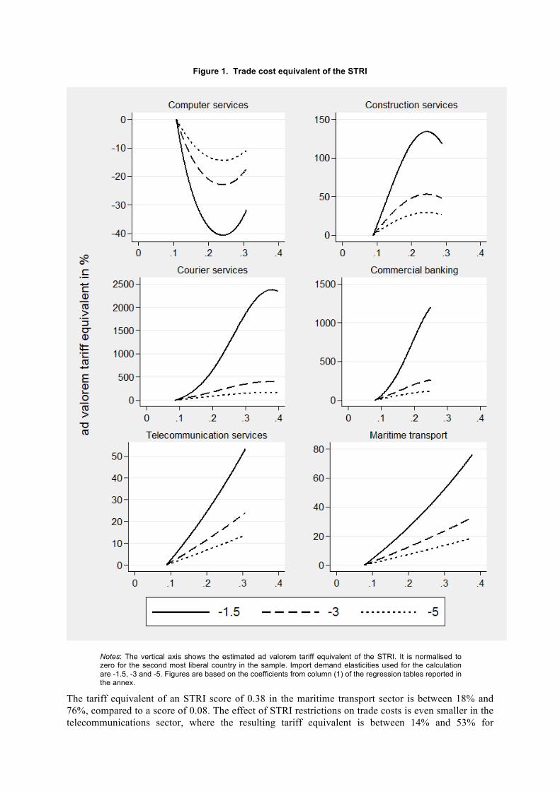
Figure 1. Trade cost equivalent of the STRI

Notes: The vertical axis shows the estimated ad valorem tariff equivalent of the STRI. It is normalised to zero for the second most liberal country in the sample. Import demand elasticities used for the calculation are -1.5, -3 and -5. Figures are based on the coefficients from column (1) of the regression tables reported in the annex.

The tariff equivalent of an STRI score of 0.38 in the maritime transport sector is between 18% and 76%, compared to a score of 0.08. The effect of STRI restrictions on trade costs is even smaller in the telecommunications sector, where the resulting tariff equivalent is between 14% and 53% for

countries with an STRI score of 0.31 relative to countries with a score of 0.09. Only a linear STRI term is used for these estimates with a regression coefficient which is not significantly different from zero at a 10% level of significance. As mentioned above, even though the coefficients are insignificant, the point estimates provide useful information on trade costs in these sectors. Moreover, reporting these results helps to avoid a selection bias which arises because large coefficients are more likely to be estimated significantly different from zero and which leads to an overestimation of the average tariff equivalent across sectors.

In the computer services sector the resulting tariff equivalent of the STRI is slightly negative. It seems that the aggregate STRI is not able to explain the pattern of cross-border services trade in this sector. This might be due to the importance of Mode 3 and Mode 4 for the STRI score in this sector, while trade in computer services is often conducted via Mode 1 without any accompanying movement of people, for example via online transfer of data.12 The subsequent parts of this report will present further analysis whether individual components of the total STRI may be able to explain the pattern of trade costs for computer services and in all other sectors.

5.2 Market access and national treatment vs. domestic regulation

All STRI measures are classified into different groups, according to the type of restriction they imply.13 These classifications are used to construct an STRI which is exclusively based on a certain type of barrier. The first distinction is made between barriers with respect to market access and national treatment of foreign suppliers, as opposed to an STRI from domestic regulation and other barriers. An intuition for these two categories is outlined in the STRI sector papers:

“As with any classification, it is not always possible to clearly identify to which category certain restrictions belong and there are overlaps in the classification of some barriers. Therefore, market access and national treatment measures are classified together. This grouping also allows a distinction to be made between restrictions subject to scheduling under the GATS and domestic regulatory measures that usually do not need to be scheduled. Restrictions not captured by either market access or national treatment are classified under domestic regulation, and other barriers. The classification is without prejudice to WTO Members’ commitments and obligations under the GATS.” (Nordås et al., 2014a) The following figures are all based on an import demand elasticity of -3 and it should be born in mind that estimates of the tariff equivalent depend strongly on the import demand elasticity. Consequently, these estimates should not be interpreted according to their absolute values, but rather with respect to the relative importance of the different groups of restrictions in each sector.

12 The currently ongoing 2016 update of the STRI will add more measures that capture restrictions to Mode 1. In

particular, restrictions on data transfer will be included which might constitute significant barriers to cross-border trade in computer services.

13 A complete list of all measures and their classification with respect to these categories as well as the resulting STRI scores can be found in the STRI sector papers published as Geloso Grosso et al. (2014a, 2014b, 2014c), Nordås et al. (2014a, 2014b, 2014c), Rouzet et al. (2014) and Ueno et al. (2014).

Figure 2. Market access and national treatment vs. domestic regulation

Notes: The vertical axis shows the estimated ad valorem tariff equivalent of the STRI. It is normalised to zero for the second most liberal country in the sample. Import demand elasticity used for the calculation -3. Figures are based on the coefficients from column (3) of the regression tables reported in the annex.

The contribution of market access and national treatment barriers to services trade costs relative to the contribution of domestic regulation differs substantially across sectors. Only in the commercial banking sector do market access and national treatment restrictions account for the major part of the barriers to cross-border trade, while domestic regulation does not constitute a significant tariff equivalent in that sector. Consequently, only a liberalisation which facilitates market access and national treatment can contribute to a reduction of trade barriers for commercial banking services. Moreover, it can be seen that the relationship of the STRI and estimated trade costs flattens for high levels of restrictions. This pattern implies that the marginal impact of additional barriers on trade costs falls with a rising STRI score. Taking an opposite view, it means that a liberalisation of market access and national treatment barriers from 0.05 to 0.04 induces a stronger reduction of trade costs than a liberalisation from 0.15 to 0.14.

In the courier services sector both groups of measures contribute to trade costs. However, the relationship between STRI barriers and the estimated tariff equivalent differs substantially between the two groups. Domestic regulation only represents trade costs for very high levels of restrictiveness. At the same time, market access and national treatment constitute the highest level of trade costs for an STRI score of around 0.13, while additional barriers do not increase trade costs further. This pattern implies that in the vast majority of countries barriers to market access and national treatment represent higher trade costs than domestic regulation and other barriers. The liberalisation of market access and national treatment should be the focus of policy reforms in those countries in order to facilitate services trade. Only countries with a very high STRI of which more than 0.2 comes from measures related to domestic regulation should place emphasis on the liberalisation of domestic regulation.

In contrast, domestic regulation is responsible for the major part of services trade costs in the remaining four sectors. These sectors are computer services, construction services, telecommunication services14 and maritime transport. This result highlights the burden of costly adjustment to domestic regulation in a high number of countries to which firms export. There exist several distinct patterns with respect to the trade cost effect of domestic regulation.

For example, only very restrictive domestic regulation seems to constitute trade costs in the computer services sector, while in the construction services sector additional restrictions above a score of 0.1 do not lead to a further increase of trade costs. The possibility to export computer services via the internet might provoke this pattern, because foreign suppliers who provide their services online are not affected by many aspects of domestic regulation in the importing country.15 In contrast, construction services suppliers are much more exposed to domestic regulation in the importing country, for example requirements to access public procurement contracts or differences in building standards and qualification requirements, so that significant trade costs may arise from just few of these restrictions. This explains why measures related to domestic regulation have a stronger impact on trade in construction services (and trade in maritime transport) than trade in computer services. The difference is especially pronounced for low levels of restrictiveness.

14 In the telecommunications sector this result is based on regression coefficients which are not different from

zero at the conventional levels of significance. 15 Restrictions to data transfer might be an important determinant of cross-border trade in computer services.

This aspect can be analysed after the completion of the 2016 STRI.

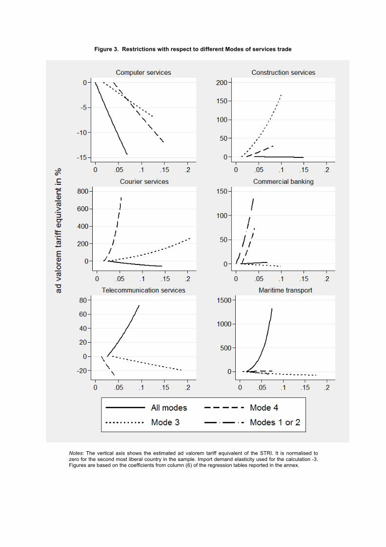
Figure 3. Restrictions with respect to different Modes of services trade


5.3 Restrictions with respects to different Modes of services trade

The disaggregation of the STRI also allows for an analysis of restrictions to different modes of services trade. These Modes are, Mode 1: Cross-border supply; Mode 2: Consumption abroad; Mode 3: Commercial presence; and Mode 4: Temporary movement of natural persons. In the STRI database measures are classified to either affect all Modes of services trade, to affect only Mode 3, only Mode 4, or Modes 1 and 2. The last group, however, is only included in the STRI for commercial banking and maritime transport among the sectors analysed here. In the other four sectors, no policy measures could be identified which apply predominantly to Modes 1 and 2. Very often, different modes of trade in services are complementary to each other, for example when natural persons in a foreign economy provide services in collaboration with colleagues from their home country who export services via Mode 1. This means that all measures to the movement of people also affect trade in services via Mode 1. However, when measures can affect trade in services via different modes, they are classified according to the Mode which they affect most. In the example above, restrictions to the movement of people are classified as barriers to Mode 4.

Data on cross-border trade in services from the balance of payments broadly cover Modes 1, 2 and 4, with the additional limitation that the services of self-employed suppliers staying in the host economy for a year or longer are not included, since these suppliers become residents of the host country. Nevertheless, also measures related to Mode 3 of services trade can affect cross-border trade. On the one hand, services provided via different Modes may be substitutes, so that additional barriers to Mode 3 make cross-border trade relatively more attractive. Such a situation would be captured by a negative tariff equivalent of barriers to Mode 3. On the other hand, services are often supplied via a combination of different Modes, so that restrictions to Mode 3 also constitute barriers for the supply of services across the border. In this case, the resulting tariff equivalent of barriers to Mode 3 should be positive.

In line with these conflicting alternatives, the impact of barriers to Mode 3 on trade costs differs substantially across sectors.16 Such barriers constitute positive trade costs in the construction and courier services sector, which means that Mode 3 is complementary to other Modes of services trade in these sectors. This result seems particularly intuitive in the construction sector, where cross-border trade of construction materials is often recorded as trade in construction services which is complementary to the establishment of construction sites abroad via Mode 3. In all other sectors, barriers to Mode 3 represent negative tariff equivalents but the coefficient is only significantly negative in the maritime transport sector. It implies that additional barriers of this type increase the volume of cross-border trade so that Mode 3 is a substitute to other Modes of services trade.

Barriers to Mode 4 of services trade which are captured in the STRI constitute high trade costs in the courier services and the commercial banking sector. In these sectors, barriers to Mode 4 are among the most important restrictions to cross-border trade. While this seems natural for a labour-intensive industry such as courier services, there is no intuitive explanation for the importance of Mode 4 barriers for trade in commercial banking. In all other sector, the regression coefficients are not statistically significant from zero. Behind-the-border barriers which affect all Modes constitute trade costs in the telecommunication and the maritime transport sector. In particular in maritime transport these barriers seem to be very important and represent by far the largest share of total trade costs. Barriers to Modes 1 and 2 are only included in the STRI of two sectors. They represent significant costs for cross-border trade only in the banking sector. In this sector, this type of barriers represents higher trade costs than barriers of any other type, while they have an insignificant effect in the maritime transport sector.

16 Quadratic terms cannot be included in this regression which implies that the lines in Figure 4 are exponential

functions by construction.

Figure 4. Discriminatory vs. non-discriminatory measures


5.4 Discriminatory measures vs. non-discriminatory measures

The measures in the STRI database can also be distinguished with respect to their effect on the competition between domestic services providers and foreign providers. Discriminatory measures affect the conditions of services provisions in favour of domestic suppliers so that demand is shifted towards them. In contrast, non-discriminatory measures affect domestic and foreign suppliers similarly, raising the cost for all services providers, resulting in higher prices and lower demand for services in general.

Discriminatory barriers only represent substantial trade barriers in two of the six sectors, the courier services and commercial banking sector. In these sectors such discriminatory barriers have a particularly large effect on trade costs when the level of restrictions is low. The marginal effect of additional barriers on trade costs vanishes with the amount of restrictions in place. In all other sectors, the effect of discriminatory barriers on trade costs is not significantly different from zero.

The pattern in the courier services sector is particularly interesting, because discriminatory barriers appear to be small, relative to non-discriminatory barriers. However, for almost the entire range of services trade restrictions, discriminatory barriers represent higher trade costs than non-discriminatory barriers, which only seem to become relevant when they constitute a very high STRI score. Similar to the disaggregation into market access and national treatment vs. domestic regulation and other barriers, this pattern suggests that discriminatory trade barriers in the courier services sector account for the major part of services trade costs in almost all countries.

Non-discriminatory barriers to services trade represent restrictions in almost all sectors. Regression coefficients are sometimes not statistically significant at the 10% level, but usually they are at a 20% level of significance.17 Low levels of non-discriminatory barriers do not constitute significant trade costs in three of the six sectors, computer services, courier services and commercial banking, while a restrictive framework of non-discriminatory regulation does constitute high barriers to cross-border services trade in all sectors. This stands in contrast to the pattern for discriminatory barriers, where an intermediate level of restrictiveness implies the highest value of services trade costs in three of the six sectors. This analysis indicates that a considerable share of the aggregate tariff equivalent of the STRI is due to non-discriminatory measures and the contribution of non-discriminatory measures is particularly high in countries with a high STRI score.

5.5 Establishment barriers vs. barriers to operations

Establishment barriers and barriers to operations affect services suppliers at different stages in the process of delivering services to a foreign country. “Establishment restrictions can generally be regarded as impediments to the movement of factors of production, while those applying to firms’ operations constrain service provision after establishment” (Nordås et al., 2014a). Consequently, measures are classified as establishment barriers, if they restrict or prevent the establishment of new trading relationships and these restrictions represent additional cost of entering into an export market for services exporters. Barriers to the operations of services suppliers restrict the ability of services suppliers to maintain their operations in an export market and represent additional costs in order to retain existing export relationships.18

17 The only exception is the telecommunication sector, where the coefficients are clearly insignificant. 18 Establishment barriers might be associated with fixed export costs, which do not depend on the level of

exports to a particular destination, while barriers to operations might constitute variable export costs which depend on the quantity of services exports. However, it is only possible to answer this question with trade data on the firm level. The importance of establishment barriers complicates the interpretation of trade costs as ad valorem tariff equivalent when the size of such barriers does not depend on the volume of services trade.

Figure 5. Establishment barriers vs. barriers to operations


Trade costs are mostly due to establishment barriers in three of the six sectors: courier services, commercial banking and maritime transport.19 In the courier services and commercial banking sector low STRI scores already represent substantial tariff equivalents while the marginal costs to adding additional barriers falls as the level of trade restrictiveness increases. This implies that a substantial liberalisation is needed in order to reduce services trade costs in these sectors when a country starts out in a relatively restrictive environment because only a small effect on trade costs can be expected from a liberalisation when trade remains relatively restrictive. In contrast, in the maritime transport sector only very high levels of discriminatory trade barriers represent a significantly positive tariff equivalent while restrictions up to an STRI score of around 0.15 do not have any effect on trade costs.

The importance of establishment barriers in these three sectors suggests that a reduction of services trade barriers may benefit small and medium enterprises in particular. The reason is that the cost to overcome such establishment barriers may be independent of the sales volume of services providers.20 This implies that large firms find it easier to recover these costs when delivering large quantities across the border, while small firms with lower sales volumes might not be able to recover the costs of establishment in an export market and abstain from entering foreign markets in the first place. A reduction of services trade barriers would then be able to raise the share of exporting firms among all services providers.

Similarly, there arise substantial differences across sectors with respect to trade costs from barriers to operations of services suppliers. For example, in the construction sector barriers to operations represent a high tariff equivalent. However, additional barriers do only raise trade costs up to an STRI score of 0.13. An equivalent interpretation is that a removal of restrictions which does not bring the score down to at least 0.13 cannot contribute to a reduction of trade costs in the sector. In contrast, in the courier services sector barriers to operations only constitute trade costs if they represent an STRI score of more than 0.15. Up to this score, trade costs from barriers to operations remain close to zero. In most other sectors, barrier to operations only have a negligible impact on services trade costs.

7. Concluding remarks

This report presents preliminary evidence on the contribution of services trade restrictions to trade costs for cross-border trade in services. Estimated ad valorem tariff equivalents of the STRI depend strongly on the underlying import demand elasticities. Best estimates for their values lie between 162% and 2377% for courier services, between 116% and 1203% for commercial banking services, between 29% and 134% for construction services, between 18% and 76% in the maritime transport sector, and between 14% and 53% for telecommunication services Trade costs do not increase linearly with a country’s STRI score in many sectors. For example, in the construction sector a pronounced drop in trade costs can be achieved by reducing barriers from 0.2 to 0.1, while a reduction from 0.3 to 0.2 does not contribute to a significant reduction of trade costs.

Moreover, the report shows that different types of regulatory policies contribute unequally to services trade costs even when they account for identical STRI scores. The patterns differ substantially across sectors. When comparing results from individual regressions on the sector-level, it is possible to identify similarities between the courier services sector and the commercial banking sector with respect to the composition of services trade costs. In both sectors, cross-border trade in services in the majority of are mostly due to market access and national treatment barriers, discriminatory measures and establishment barriers.

Likewise, the construction sector and the maritime transport sector seem to be relatively similar. In both sectors, a reduction of services trade costs should focus a liberalisation of domestic regulation

19 In the courier services sector, the tariff equivalent in countries with very high STRI scores comes

predominantly from barriers to the operations of foreign suppliers. 20 However, such an interpretation of services trade costs stands in contrast with an ad valorem tariff equivalent

as meaningful indicator of services trade costs.

and other barriers and a liberalisation of non-discriminatory measures. In the computer services and telecommunication services sectors, coefficients are often insignificant and substantially smaller.

The report does not cover Mode 3 of services trade, the commercial presence of services suppliers, which is a quantitatively very important component of total trade in services. This is due to the fact that these trade flows are not registered in a country’s balance of payments. Instead, an estimation of trade costs for Mode 3 of services trade must rely on firm-level information on foreign affiliate sales. Acknowledging the importance of Mode 3 for a complete description of the costs of services trade, that type of analysis remains for future research.

Further progress from future research should be expected from the availability of additional data on services trade restrictions and services trade. It is a limitation that a country’s STRI score from 2014 must be used to represent trade costs between 2010 and 2013. With the availability of trade data for the years from 2014 onwards this problem can be substantially mitigated. Even more importantly, with the availability of trade data from 2015 onwards, panel estimation techniques can be used to derive the effect of changes in the STRI over time on services trade flows. This can further improve the robustness of the estimated results. However, it must be noted that the feasibility of such an analysis hinges on the incidence of actual changes in services trade restrictions over time.

This report constitutes one element of a suite of studies which are currently conducted at the OECD with the common objective to explore alternative ways to estimate the costs associated with services trade restrictions. Other studies determine the role of regulatory heterogeneity for trade costs, they analyse the impact of services trade restrictions on the level of domestic competition and they study to which degree these barriers restrict trade in services via Mode 3 using data on foreign affiliate sales. Hence, the results in this paper should not be considered as final evidence on the costs of services trade restrictions. Further evidence on different aspects of services trade costs will be made available in the future in order to complement these results. Moreover, newly available data on services trade and services trade restrictions over time might allow for more robust estimates in the future.

REFERENCES

Anderson, James E., Catherine A. Milot and Yoto V. Yotov (2014), “How Much Does Geography Deflect Services Trade? Canadian Answers”, International Economic Review, 55: 791–818

Anderson, James E. and Eric van Wincoop (2003), “Gravity with Gravitas: A Solution to the Border Puzzle”, American Economic Review, 93(1): 170-192.

Anderson, James E. and Eric van Wincoop (2004), “Trade Costs”, Journal of Economic Literature, 42(3): 691-751

Ariu, Andrea and Giordano Mion (2012), “Trade in Services and Occupational Tasks: An Empirical Investigation”, CEPR Working Paper 8761

Arkolakis, Costas, Arnaud Costinot and Andres Rodriguez-Clare (2012), “New trade models, same old gains?”, American Economic Review, 102: 94–130

Baier, Scott L. and Jeffrey H. Bergstrand (2007), “Do free trade agreements actually increase members' international trade?”, Journal of International Economics, 71(1): 72–95

Berden, Koen, Joseph Francois, Martin Thelle, Paul Wymenga and Saara Tamminen (2009), “Non-Tariff Measures in EU-US Trade and Investment – An Economic Analysis” Reference: OJ 2007/S 180-219493, Ecorys

Borchert, Ingo, Batshur Gootiiz and Aaditya Mattoo (2013), “Policy Barriers to International Trade in Services: Evidence from a New Database” World Bank Economic Review

Breinlich, Holger (2010), “The Elasticity of Substitution between Differentiated Traded Services: Estimates for Major Services Categories”, mimeo

Breinlich, Holger and Chiara Criscuolo (2011), “International Trade in Services: a Portrait of Importers and Exporters”, Journal of International Economics 84 (2): 188–206

Broda, Christian and David E. Weinstein (2006), “Globalization and the Gains From Variety”, Quarterly Journal of Economics, 121(2): 541-585.

Chen, Natalie A. (2004), “Intra-National Versus International Trade in the European Union: Why Do National Borders Matter?”, Journal of International Economics, 63(1): 93-118.

Christen, Elisabeth and Joseph Francois (2015), “Modes of Supply for US Exports of Services”, The World Economy, DOI: http://dx.doi.org/10.1111/twec.12330

Crozet, Matthieu and Emmanuel Milet (2014), “The Servitization of French Manufacturing Firms”, CEPII Working Papers 2014-10.

Evans, Carolyn L. (2003), “The Economic Significance of National Border Effects”, American Economic Review, 93(4): 1291-1312.

Fontagné, Lionel, Amélie Guillin and Cristina Mitaritonna (2011), “Estimation of Tariff Equivalents for the Services Sectors” CEPII working paper No 2011-24.

Geloso Grosso, Massimo et al. (2014a), “Services Trade Restrictiveness Index (STRI): Construction, Architecture and Engineering Services”, OECD Trade Policy Papers No. 170, OECD Publishing, Paris. DOI: http://dx.doi.org/10.1787/5jxt4nnd7g5h-en

Geloso Grosso, Massimo et al. (2014b), “Services Trade Restrictiveness Index (STRI): Legal and Accounting Services”, OECD Trade Policy Papers No. 171, OECD Publishing, Paris. DOI: http://dx.doi.org/10.1787/5jxt4nkg9g24-en

Geloso Grosso, Massimo et al. (2014c), “Services Trade Restrictiveness Index (STRI): Transport and Courier Services”, OECD Trade Policy Papers No. 176, OECD Publishing, Paris. DOI: http://dx.doi.org/10.1787/5jxt4nd187r6-en

Geloso Grosso, Massimo et al. (2015), “Services Trade Restrictiveness Index (STRI): Scoring and Weighting Methodology”, OECD Trade Policy Papers No. 177, OECD Publishing, Paris. DOI: http://dx.doi.org/10.1787/5js7n8wbtk9r-en

Guillin, Amélie (2013), “Assessment of tariff equivalents for services considering the zero flows”, World Trade Review, 12(03): 549-575

Head, Keith, Thierry Mayer and John Ries (2010), “The erosion of colonial trade linkages after independence”, Journal of International Economics, 81(1): 1-14

Kelle, Markus and Jörn Kleinert (2010), “German Firms in Service Trade”, Applied Economics Quarterly (formerly: Konjunkturpolitik), 56 (1): 51–72

Mayer, Thierry and Soledad Zignago (2011), “Notes on CEPII’s distances measures: The GeoDist database”, CEPII Working Paper No. 2011-25.

Miroudot, Sébastien, Jehan Sauvage and Ben Shepherd (2013), “Measuring the cost of international trade in services”, World Trade Review, 12: 719-735

Miroudot, Sébastien and Ben Shepherd (2015), “Regional Trade Agreements and Trade Costs in Services”, RSCAS Working Paper 2015/85, European University Institute

Nordås, Hildegunn K. (2016), “Services Trade Restrictiveness Index (STRI): The Trade Effect of Regulatory Differences”, OECD Trade Policy Papers, No. 189, OECD Publishing, Paris. DOI: http://dx.doi.org/10.1787/5jlz9z022plp-en

Nordås, Hildegunn K. et al. (2014a), “Services Trade Restrictiveness Index (STRI): Computer and Related Services”, OECD Trade Policy Papers No. 169, OECD Publishing, Paris. DOI: http://dx.doi.org/10.1787/5jxt4np1pjzt-en

Nordås, Hildegunn K. et al. (2014b), “Services Trade Restrictiveness Index (STRI): Telecommunication Services”, OECD Trade Policy Papers No. 172, OECD Publishing, Paris. DOI: http://dx.doi.org/10.1787/5jxt4nk5j7xp-en

Nordås, Hildegunn K. et al. (2014c), “Services Trade Restrictiveness Index (STRI): Audio-visual Services”, OECD Trade Policy Papers No. 174, OECD Publishing, Paris. DOI: http://dx.doi.org/10.1787/5jxt4nj4fc22-en

Nordås, Hildegunn K. and Dorothée Rouzet (2015), “The Impact of Services Trade Restrictiveness on Trade Flows: First Estimates”, OECD Trade Policy Paper No. 178, OECD Publishing, Paris. DOI: http://dx.doi.org/10.1787/5js6ds9b6kjb-en

Puhani, Patrick (2000), “The Heckman Correction for Sample Selection and its Critique”, Journal of Economic Surveys, 14: 53-68

Rouzet, Dorothée et al. (2014), “Services Trade Restrictiveness Index (STRI): Financial Services”, OECD Trade Policy Papers No. 175, OECD Publishing, Paris. DOI: http://dx.doi.org/10.1787/5jxt4nhssd30-en

Santos Silva, J.M.C. and Silvana Tenreyro (2006), “The Log of Gravity”, The Review of Economics and Statistics, 88(4): 641-658.

Ueno, Asako et al. (2014), “Services Trade Restrictiveness Index (STRI): Distribution Services”, OECD Trade Policy Papers No. 173, OECD Publishing, Paris. DOI: http://dx.doi.org/10.1787/5jxt4njvtfbx-en

Van der Marel, Erik and Ben Shepherd (2013), “Services Trade, Regulation and Regional Integration: Evidence from Sectoral Data” World Economy, 36: 1393–1405

Walter, Patricia and Rene Dell’mour (2010), “Firm-Level Analysis of International Trade in Services”, IFC Working Papers No. 4

Wei, Shang-Jin (1996), “Intra-National versus International Trade: How Stubborn Are Nations in Global Integration?”, NBER Working Paper 5531.

ANNEX

This annex contains regression tables on which graphical results in the main part of the report are based. For each sector, results from six different specifications are reported in three separate regression tables. The main regression tables contain the coefficients on the STRI variables which differ across specifications. All coefficients in the main regression tables refer to the interaction of an STRI variable with the border-dummy, which indicates that exporter and importer are not identical countries. A second regression table for each sector reports coefficients on the interaction of the STRI variables with the intra EEA dummy, while a third regression table for each sector reports coefficients on the gravity control variables which are identical in all six specifications.

Column (1) of each table reports results on the aggregate STRI, using a linear term and a quadratic term where the quadratic term is significant. Column (2) reports the interaction of the STRI with observable country characteristics, GDP, GDP per capita and geographic size. Columns (3) to (6) report estimation results based on the decomposition of the aggregate STRI score into different groups.

The estimated pseudo R-squared is not reported due to space constraints and low informative value. It is very high (>0.99) in all specifications due to the high number of dummy variables.

Table 2. Computer services: regression results

(1) (2) (3) (4) (5) (6) b * stri 21.75** -92.20*** (10.35) (27.46) b * stri^2 -45.31* -32.82 (26.97) (35.32) b * stri * lnGDP 3.03*** (1.03) b * stri * lnGDPpc 6.06** (2.64) b * stri * lnDist 0.53 (1.52) b * DRO 56.00** (21.95) b * DRO^2 -443.48*** (143.82) b * MANT 16.85* (9.83) b * MANT^2 -33.88 (40.78) b * DIS 20.35 (13.52) b * DIS^2 -47.74 (41.60) b * NDIS 55.43*** (14.30) b * NDIS^2 -544.51*** (110.71) b * EST 2.94 (20.82) b * EST^2 2.54 (110.44) b * OPE 38.66** (17.31) b * OPE^2 -175.57* (93.48) b * All Modes 6.75 (9.74) b * Mode 3 1.99 (6.06) b * Mode 4 3.50 (4.35) Gravity Controls Yes Yes Yes Yes Yes Yes Intra EU Controls Yes Yes Yes Yes Yes Yes Exp * Year FE Yes Yes Yes Yes Yes Yes Imp * Year FE Yes Yes Yes Yes Yes Yes N 4237 4237 4237 4237 4237 4237

Notes: Dependent variable is the volume of exports. Standard errors clustered by importer. ***, ** and * mean statistical significance at 1%, 5% and 10% levels respectively. All independent variables are interactions with the border dummy. DRO: domestic regulation / other; MANT: market access / national treatment; DIS: discriminatory measures; NDIS: non-discriminatory measures; EST: establishment barriers; OPE: operations barriers.

Table 3. Computer services: Intra EU control variables

(1) (2) (3) (4) (5) (6) b * stri 9.31 36.48 (14.24) (27.86)

b * stri^2 -42.15 -69.97* (42.31) (42.24) b * stri * lnGDP -1.03 (0.82) b * stri * lnGDPpc -0.09 (2.12) b * stri * lnDist -0.38 (1.65) b * DRO -24.57 (20.28) b * DRO^2 157.91 (128.83) b * MANT 2.55 (10.04) b * MANT^2 -21.33 (45.70) b * DIS -12.46 (11.65) b * DIS^2 13.73 (45.16) b * NDIS -8.91 (10.58) b * NDIS^2 109.16 (86.21) b * EST 40.66 (50.43) b * EST^2 -240.96 (303.63) b * OPE 3.79 (15.20) b * OPE^2 -67.92 (85.16) b * All Modes -30.23** (12.60) b * Mode 3 10.38** (5.16) b * Mode 4 -6.48 (5.40) Gravity Controls Yes Yes Yes Yes Yes Yes Exp * Year FE Yes Yes Yes Yes Yes Yes Imp * Year FE Yes Yes Yes Yes Yes Yes N 4237 4237 4237 4237 4237 4237

Notes: Dependent variable is the volume of exports. Standard errors clustered by importer. ***, ** and * mean statistical significance at 1%, 5% and 10% levels respectively. All independent variables are interactions with the intra EEA dummy and with the border dummy. DRO: domestic regulation / other; MANT: market access / national treatment; DIS: discriminatory measures; NDIS: non-discriminatory measures; EST: establishment barriers; OPE: operations barriers.

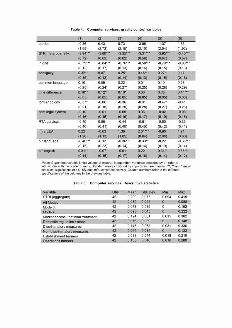
Table 4. Computer services: gravity control variables

(1) (2) (3) (4) (5) (6) border -0.36 0.43 0.73 -3.06 -1.37 1.36 (1.99) (2.72) (2.15) (2.10) (2.54) (1.92) STRI heterogeneity -3.94*** -3.60*** -3.35*** -3.31*** -3.95*** -3.40*** (0.72) (0.69) (0.62) (0.58) (0.67) (0.67) ln dist -0.79*** -0.84*** -0.76*** -0.50*** -0.79*** -0.90*** (0.12) (0.17) (0.13) (0.16) (0.15) (0.13) contiguity 0.32** 0.07 0.25* 0.46*** 0.27* 0.17 (0.15) (0.13) (0.14) (0.13) (0.15) (0.15) common language 0.10 0.05 0.22 0.01 0.10 0.23 (0.25) (0.24) (0.27) (0.25) (0.28) (0.29) time difference 0.10** 0.12** 0.10* 0.06 0.08 0.14*** (0.05) (0.05) (0.05) (0.05) (0.05) (0.05) former colony -0.37* -0.06 -0.36 -0.31 -0.47* -0.41 (0.21) (0.18) (0.28) (0.28) (0.27) (0.28) com legal system -0.10 -0.01 -0.05 0.03 -0.02 -0.03 (0.16) (0.16) (0.16) (0.17) (0.19) (0.16) RTA services -0.40 0.06 -0.44 -0.51 -0.50 -0.33 (0.40) (0.41) (0.40) (0.40) (0.42) (0.41) intra EEA 0.22 -0.63 1.36 2.31*** -0.90 1.21 (1.20) (1.13) (1.05) (0.84) (2.08) (0.80) b * language -0.40*** -0.13 -0.36** -0.33** -0.22 -0.38*** (0.15) (0.23) (0.14) (0.14) (0.19) (0.14) b * english 0.31** -0.07 -0.01 0.22 0.34** 0.36*** (0.14) (0.15) (0.17) (0.16) (0.14) (0.12)

Notes: Dependent variable is the volume of exports. Independent variables preceded by b * refer to interactions with the border dummy. Standard errors clustered by importer in parentheses. ***, ** and * mean statistical significance at 1%, 5% and 10% levels respectively. Column numbers refer to the different specifications of the columns in the previous table.

Table 5. Computer services: Descriptive statistics

Variable Obs. Mean Std. Dev. Min Max STRI (aggregate) 42 0.200 0.077 0.094 0.415 All Modes 42 0.032 0.024 0 0.088 Mode 3 42 0.073 0.039 0 0.192 Mode 4 42 0.095 0.045 0 0.222 Market access / national treatment 42 0.124 0.061 0.015 0.302 Domestic regulation / other 42 0.076 0.039 0 0.148 Discriminatory measures 42 0.146 0.068 0.031 0.330 Non-discriminatory measures 42 0.054 0.034 0 0.122 Establishment barriers 42 0.092 0.044 0.018 0.216 Operations barriers 42 0.108 0.046 0.016 0.208

Table 6. Construction services: regression results

(1) (2) (3) (4) (5) (6) b * stri -25.89** -115.38*** (11.95) (34.54) b * stri^2 52.95* 97.91* (31.09) (53.46) b * stri * lnGDP 7.70*** (2.29) b * stri * lnGDPpc -1.74 (3.70) b * stri * lnDist -2.79 (3.41) b * DRO -38.46** (19.31) b * DRO^2 133.20 (91.55) b * MANT -8.43 (17.23) b * MANT^2 49.28 (63.74) b * DIS -26.68 (17.34) b * DIS^2 107.31* (57.30) b * NDIS -1.75 (92.05) b * NDIS^2 -545.44 (804.57) b * EST 15.59 (22.76) b * EST^2 -207.96 (199.56) b * OPE -73.16*** (19.55) b * OPE^2 262.94*** (76.53) b * All Modes 0.52 (6.48) b * Mode 3 -33.56** (13.51) b * Mode 4 -12.99 (8.65) Gravity Controls Yes Yes Yes Yes Yes Yes Intra EU Controls Yes Yes Yes Yes Yes Yes Exp * Year FE Yes Yes Yes Yes Yes Yes Imp * Year FE Yes Yes Yes Yes Yes Yes N 4679 4679 4679 4679 4679 4679


Table 7. Construction services: Intra EU control variables

(1) (2) (3) (4) (5) (6) b * stri 15.60 96.32*** (12.94) (31.92)

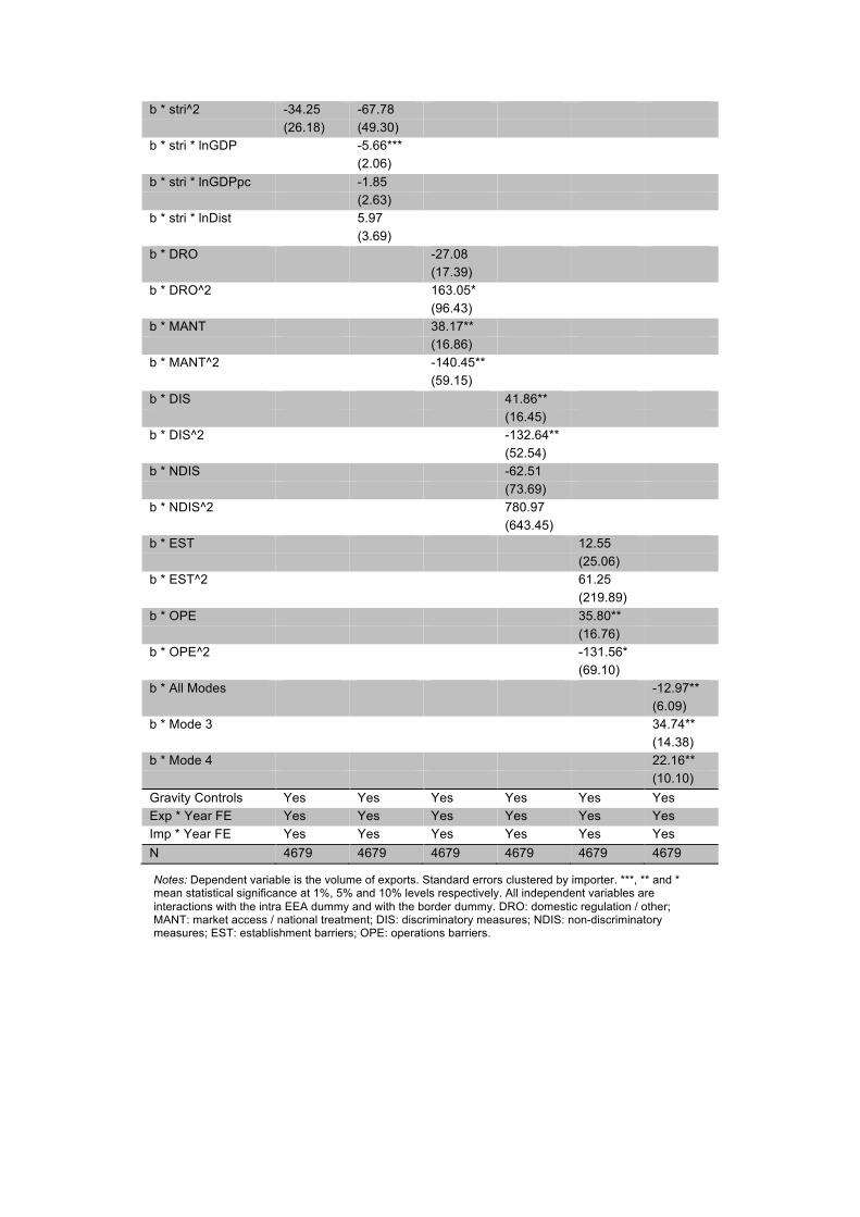
b * stri^2 -34.25 -67.78 (26.18) (49.30) b * stri * lnGDP -5.66*** (2.06) b * stri * lnGDPpc -1.85 (2.63) b * stri * lnDist 5.97 (3.69) b * DRO -27.08 (17.39) b * DRO^2 163.05* (96.43) b * MANT 38.17** (16.86) b * MANT^2 -140.45** (59.15) b * DIS 41.86** (16.45) b * DIS^2 -132.64** (52.54) b * NDIS -62.51 (73.69) b * NDIS^2 780.97 (643.45) b * EST 12.55 (25.06) b * EST^2 61.25 (219.89) b * OPE 35.80** (16.76) b * OPE^2 -131.56* (69.10) b * All Modes -12.97** (6.09) b * Mode 3 34.74** (14.38) b * Mode 4 22.16** (10.10) Gravity Controls Yes Yes Yes Yes Yes Yes Exp * Year FE Yes Yes Yes Yes Yes Yes Imp * Year FE Yes Yes Yes Yes Yes Yes N 4679 4679 4679 4679 4679 4679


Table 8. Construction services: gravity control variables

(1) (2) (3) (4) (5) (6)

border -12.02*** -18.13** -10.07** -9.60** -5.83 -11.61** (4.54) (7.71) (4.72) (4.53) (4.57) (4.53) STRI heterogeneity 1.35 0.49 1.38 0.70 1.18 2.19 (1.88) (1.62) (1.72) (1.45) (1.82) (2.02) ln dist -0.78*** -1.09*** -1.07*** -0.82*** -0.79*** -0.90*** (0.18) (0.20) (0.16) (0.15) (0.16) (0.15) contiguity 0.50*** 0.07 0.19 0.25 0.40*** 0.44*** (0.18) (0.16) (0.16) (0.17) (0.14) (0.14) common language 0.36** 0.59** 0.54*** 0.21 0.57*** 0.29* (0.16) (0.24) (0.19) (0.18) (0.22) (0.17) time difference 0.05 0.09* 0.11** 0.08 0.05 0.06 (0.05) (0.05) (0.05) (0.05) (0.05) (0.05) former colony 0.50** 0.35* 0.41** 0.60*** 0.50*** 0.40* (0.20) (0.19) (0.21) (0.18) (0.18) (0.22) com legal system 0.08 0.06 0.18 0.33** 0.13 0.19 (0.15) (0.14) (0.12) (0.13) (0.13) (0.12) RTA services 0.38 0.60 0.51 0.52 0.33 0.52 (0.44) (0.51) (0.46) (0.51) (0.50) (0.47) Intra EEA -1.65 -2.98** -1.49 -1.43 -3.16** -1.65 (1.52) (1.40) (0.97) (2.01) (1.51) (1.08) b * language -0.29 0.56** -0.52*** -0.03 -0.37** -0.21* (0.19) (0.28) (0.18) (0.14) (0.18) (0.12) b * english -0.24 -0.57*** -0.56** -0.70*** -0.36** -0.35* (0.18) (0.19) (0.25) (0.24) (0.18) (0.21) b * internet 3.41*** 4.72*** 4.20*** 3.16*** 2.67*** 3.30*** (0.82) (1.49) (1.17) (1.08) (0.84) (0.95)


Table 9. Construction services STRI: Descriptive statistics

Variable Obs. Mean Std. Dev. Min Max

STRI (aggregate) 42 0.200 0.082 0.071 0.403

All Modes 42 0.094 0.044 0.014 0.190

Mode 3 42 0.045 0.044 0 0.193

Mode 4 42 0.061 0.029 0 0.143

Market access / national treatment 42 0.106 0.054 0.015 0.275

Domestic regulation / other 42 0.094 0.042 0.027 0.202

Discriminatory measures 42 0.139 0.069 0.030 0.310

Non-discriminatory measures 42 0.060 0.024 0.026 0.126

Establishment barriers 42 0.075 0.043 0 0.207

Operations barriers 42 0.124 0.052 0.041 0.241

Table 10. Courier services: regression results

(1) (2) (3) (4) (5) (6) b * stri -42.72 -94.23** (26.52) (40.37)

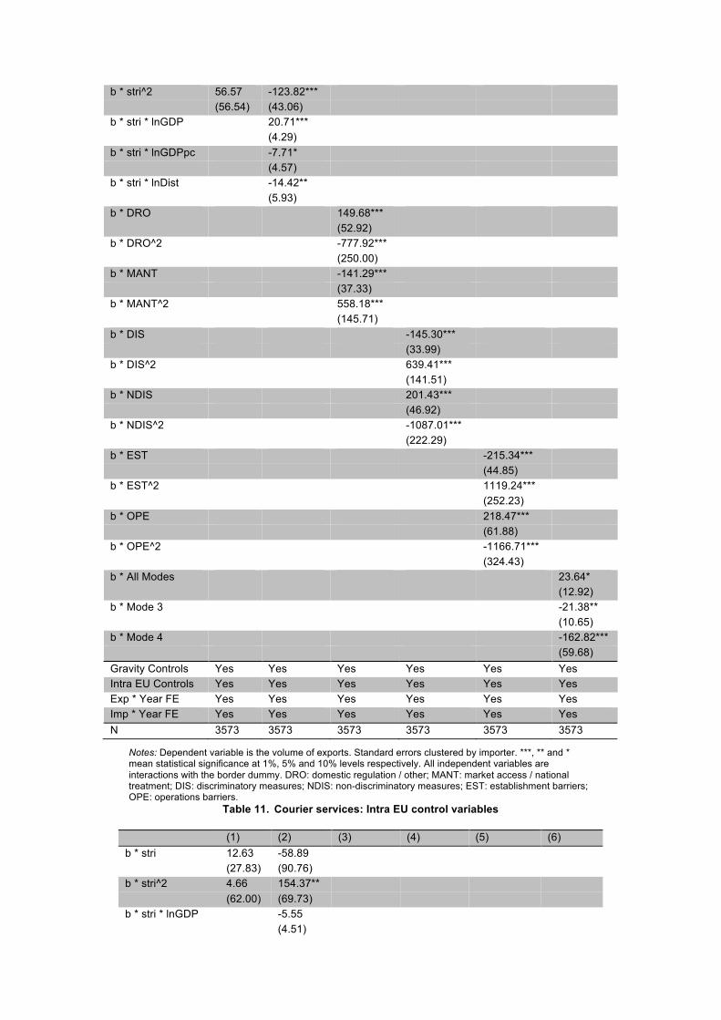
b * stri^2 56.57 -123.82*** (56.54) (43.06) b * stri * lnGDP 20.71*** (4.29) b * stri * lnGDPpc -7.71* (4.57) b * stri * lnDist -14.42** (5.93) b * DRO 149.68*** (52.92) b * DRO^2 -777.92*** (250.00) b * MANT -141.29*** (37.33) b * MANT^2 558.18*** (145.71) b * DIS -145.30*** (33.99) b * DIS^2 639.41*** (141.51) b * NDIS 201.43*** (46.92) b * NDIS^2 -1087.01*** (222.29) b * EST -215.34*** (44.85) b * EST^2 1119.24*** (252.23) b * OPE 218.47*** (61.88) b * OPE^2 -1166.71*** (324.43) b * All Modes 23.64* (12.92) b * Mode 3 -21.38** (10.65) b * Mode 4 -162.82*** (59.68) Gravity Controls Yes Yes Yes Yes Yes Yes Intra EU Controls Yes Yes Yes Yes Yes Yes Exp * Year FE Yes Yes Yes Yes Yes Yes Imp * Year FE Yes Yes Yes Yes Yes Yes N 3573 3573 3573 3573 3573 3573


Table 11. Courier services: Intra EU control variables

(1) (2) (3) (4) (5) (6) b * stri 12.63 -58.89 (27.83) (90.76) b * stri^2 4.66 154.37** (62.00) (69.73) b * stri * lnGDP -5.55 (4.51)

b * stri * lnGDPpc 7.71 (7.98) b * stri * lnDist 3.56 (7.53) b * DRO -178.73*** (50.65) b * DRO^2 930.21*** (241.07) b * MANT 48.29* (25.33) b * MANT^2 -202.59** (101.44) b * DIS 52.55** (25.22) b * DIS^2 -234.39** (99.31) b * NDIS -214.50*** (45.21) b * NDIS^2 1133.70*** (217.01) b * EST 103.75*** (38.46) b * EST^2 -629.71*** (241.20) b * OPE -216.76*** (61.61) b * OPE^2 1188.55*** (323.93) b * All Modes 12.77 (18.51) b * Mode 3 1.44 (13.16) b * Mode 4 42.05 (58.31) Gravity Controls Yes Yes Yes Yes Yes Yes Exp * Year FE Yes Yes Yes Yes Yes Yes Imp * Year FE Yes Yes Yes Yes Yes Yes N 3573 3573 3573 3573 3573 3573


Table 12. Courier services: gravity control variables

(1) (2) (3) (4) (5) (6) border -10.80 -20.28*** -5.26 2.59 3.29 -14.80** (6.76) (3.89) (6.42) (6.76) (6.34) (6.98) STRI heterogeneity -9.14* -4.66 -7.21** -5.08 -7.89** -7.53** (4.75) (3.51) (2.99) (3.15) (3.38) (3.17) ln dist -0.13 -0.95*** -0.43 -0.72*** -0.46** -0.23 (0.32) (0.33) (0.27) (0.24) (0.23) (0.32) contiguity 1.45*** 0.28 1.14*** 0.74** 0.92*** 1.06*** (0.30) (0.37) (0.36) (0.33) (0.31) (0.27) common language 0.62 -0.03 1.09** 1.02** 0.86** 0.81* (0.46) (0.45) (0.49) (0.45) (0.40) (0.45) time difference 0.24** 0.23* 0.40*** 0.37*** 0.31*** 0.03 (0.10) (0.14) (0.11) (0.09) (0.08) (0.11) former colony -2.70** -2.31** -2.36*** -1.90** -1.81** -2.36** (1.14) (0.95) (0.91) (0.82) (0.83) (1.05) com legal system 0.03 0.41* 0.09 0.11 0.02 0.15 (0.24) (0.24) (0.18) (0.19) (0.18) (0.19) RTA services 1.10 3.56*** 3.33*** 4.64*** 4.43*** 1.16* (0.81) (0.80) (0.66) (0.80) (0.85) (0.64) Intra EEA -4.62** -5.16** 0.73 -0.28 -1.98 -6.71*** (2.21) (2.11) (2.46) (2.31) (2.52) (2.31) b * language -0.46 2.16*** -0.60* -0.40 -0.30 0.59** (0.29) (0.30) (0.31) (0.26) (0.24) (0.27) b * english 0.09 -0.81*** 0.95** 0.45 0.56 0.84** (0.25) (0.24) (0.42) (0.42) (0.46) (0.34) b * internet 3.49*** 2.76*** 0.22 -1.00 -1.25 2.21** (1.17) (0.91) (1.26) (1.34) (1.35) (1.10)


Table 13. Courier services: Descriptive statistics


STRI (aggregate) 42 0.257 0.170 0.070 0.868

All Modes 42 0.087 0.054 0.012 0.239

Mode 3 42 0.131 0.108 0 0.544

Mode 4 42 0.039 0.019 0 0.086

Market access / national treatment 42 0.119 0.102 0 0.506


Discriminatory measures 42 0.115 0.094 0 0.448


Establishment barriers 42 0.110 0.076 0.012 0.390

Operations barriers 42 0.147 0.099 0.031 0.479 Table 14. Telecommunication services: regression results

(1) (2) (3) (4) (5) (6) b * stri -2.93 -79.11** (2.55) (31.98) b * stri^2 -26.30

(23.51) b * stri * lnGDP 2.74 (1.77) b * stri * lnGDPpc 1.09 (2.12) b * stri * lnDist 6.69* (4.02) b * DRO -12.57 (24.18) b * DRO^2 24.65 (102.44) b * MANT 20.42 (15.57) b * MANT^2 -110.48 (77.17) b * DIS 6.15 (16.01) b * DIS^2 -47.68 (78.52) b * NDIS -2.81 (27.80) b * NDIS^2 -9.63 (124.18) b * EST 8.31 (17.20) b * EST^2 -67.46 (100.37) b * OPE -4.77 (22.41) b * OPE^2 2.56 (88.22) b * All Modes -23.73** (11.69) b * Mode 3 4.35 (6.78) b * Mode 4 32.35 (20.12) Gravity Controls Yes Yes Yes Yes Yes Yes Intra EU Controls Yes Yes Yes Yes Yes Yes Exp * Year FE Yes Yes Yes Yes Yes Yes Imp * Year FE Yes Yes Yes Yes Yes Yes N 4079 4079 4079 4079 4079 4079


Table 15. Telecommunication services: Intra EU control variables

(1) (2) (3) (4) (5) (6) b * stri 1.31 93.31*** (3.24) (32.08) b * stri^2 -296.46** (129.55) b * stri * lnGDP -1.44 (1.68) b * stri * lnGDPpc 0.49

(2.36) b * stri * lnDist -0.46 (3.20) b * DRO 90.25*** (26.74) b * DRO^2 -493.90*** (149.04) b * MANT 8.65 (17.14) b * MANT^2 -142.37 (148.78) b * DIS 34.26 (30.98) b * DIS^2 -334.58 (270.49) b * NDIS 95.08*** (34.64) b * NDIS^2 -566.55*** (209.90) b * EST 17.75 (28.17) b * EST^2 -279.21 (275.51) b * OPE 102.59*** (23.65) b * OPE^2 -515.63*** (112.93) b * All Modes 12.57 (9.51) b * Mode 3 -4.31 (4.71) b * Mode 4 9.54 (15.22) Gravity Controls Yes Yes Yes Yes Yes Yes Exp * Year FE Yes Yes Yes Yes Yes Yes Imp * Year FE Yes Yes Yes Yes Yes Yes N 4079 4079 4079 4079 4079 4079


Table 16. Telecommunication services: gravity control variables

(1) (2) (3) (4) (5) (6) border 2.12 0.64 2.93 2.40 0.03 3.59* (1.78) (1.68) (2.34) (2.35) (2.29) (1.86) STRI heterogeneity -5.33*** -3.60*** -4.35*** -4.84*** -5.18*** -4.55*** (1.22) (1.21) (1.22) (1.14) (1.17) (1.41) ln dist -0.74*** -1.06*** -0.85*** -0.74*** -0.57*** -1.01*** (0.19) (0.22) (0.17) (0.15) (0.17) (0.19) contiguity 0.22 -0.18 0.12 0.18 0.26 -0.03 (0.18) (0.20) (0.16) (0.14) (0.18) (0.19) common language 0.63*** 0.68*** 0.49*** 0.45*** 0.43*** 0.58*** (0.13) (0.17) (0.12) (0.12) (0.16) (0.13) time difference -0.12** -0.07 -0.12*** -0.13*** -0.16*** -0.10* (0.05) (0.05) (0.05) (0.04) (0.04) (0.06) former colony -0.59*** -0.53*** -0.54*** -0.47*** -0.57*** -0.55*** (0.14) (0.17) (0.14) (0.14) (0.15) (0.15) com legal system 0.10 0.21* 0.19 0.18 0.20 0.12 (0.12) (0.11) (0.12) (0.12) (0.14) (0.12) RTA services 0.18 0.08 0.31 0.24 0.05 0.43 (0.37) (0.30) (0.32) (0.32) (0.35) (0.36) Intra EEA -0.36 -4.95** -4.17*** -4.76*** -5.07*** -0.69 (0.72) (2.32) (1.46) (1.63) (1.43) (0.78) b * language -0.84*** -0.39** -0.78*** -0.80*** -0.72*** -0.82*** (0.12) (0.20) (0.11) (0.12) (0.11) (0.12) b * english 0.71*** 0.69*** 0.58*** 0.58*** 0.70*** 0.59*** (0.10) (0.09) (0.09) (0.08) (0.10) (0.10)


Table 17. Telecommunication services: Descriptive statistics

Variable Obs. Mean Std. Dev. Min Max STRI (aggregate) 42 0.228 0.136 0.080 0.569 All Modes 42 0.080 0.055 0.020 0.238 Mode 3 42 0.120 0.085 0.029 0.342 Mode 4 42 0.028 0.013 0 0.062 Market access / national treatment 42 0.093 0.069 0.010 0.253 Domestic regulation / other 42 0.136 0.083 0.036 0.354 Discriminatory 42 0.103 0.074 0.016 0.271 Non-discriminatory 42 0.125 0.077 0.030 0.330 Establishment 42 0.080 0.059 0.015 0.211 Operations 42 0.148 0.088 0.036 0.369

Table 18. Maritime transport: regression results

(1) (2) (3) (4) (5) (6) b * stri -2.84 -69.89 (2.64) (125.21) b * stri^2 -26.25 (54.50) b * stri * lnGDP 7.94** (3.71) b * stri * lnGDPpc 7.11 (14.75) b * stri * lnDist -16.51 (12.84) b * DRO -181.40*** (67.44) b * MANT 60.63 (49.29) b * MANT^2 -136.10 (109.42) b * DIS 91.98* (48.31) b * DIS^2 -235.61** (106.49) b * NDIS -223.75*** (72.66) b * EST 152.22 (158.16) b * EST^2 -680.36 (675.91) b * OPE -26.33 (93.67) b * OPE^2 524.35 (803.33) b * All Modes -135.11*** (32.58) b * Mode 3 28.65** (12.60) b * Mode 4 -5.41 (40.27) b * Modes 1/2 45.93 (38.93) Gravity Controls Yes Yes Yes Yes Yes Yes Intra EU Controls Yes Yes Yes Yes Yes Yes Exp * Year FE Yes Yes Yes Yes Yes Yes Imp * Year FE Yes Yes Yes Yes Yes Yes N 2488 2488 2488 2488 2488 2488


Table 19. Maritime transport: Intra EU control variables

(1) (2) (3) (4) (5) (6) b * stri -1.26 173.02 (4.77) (111.48) b * stri^2 -138.77** (59.27)

b * stri * lnGDP 0.15 (4.24) b * stri * lnGDPpc -11.23 (10.90) b * stri * lnDist -2.13 (11.58) b * DRO 14.58 (32.47) b * MANT 14.69 (37.81) b * MANT^2 -65.82 (105.78) b * DIS -19.26 (33.41) b * DIS^2 49.15 (93.49) b * NDIS 16.23 (25.44) b * EST 2.91 (121.23) b * EST^2 72.53 (508.50) b * OPE -90.93 (106.92) b * OPE^2 480.64 (875.51) b * All Modes 34.30** (16.33) b * Mode 3 -11.09*** (4.11) b * Mode 4 0.70 (39.58) b * Modes 1/2 95.57* (54.51) Gravity Controls Yes Yes Yes Yes Yes Yes Exp * Year FE Yes Yes Yes Yes Yes Yes Imp * Year FE Yes Yes Yes Yes Yes Yes N 2488 2488 2488 2488 2488 2488


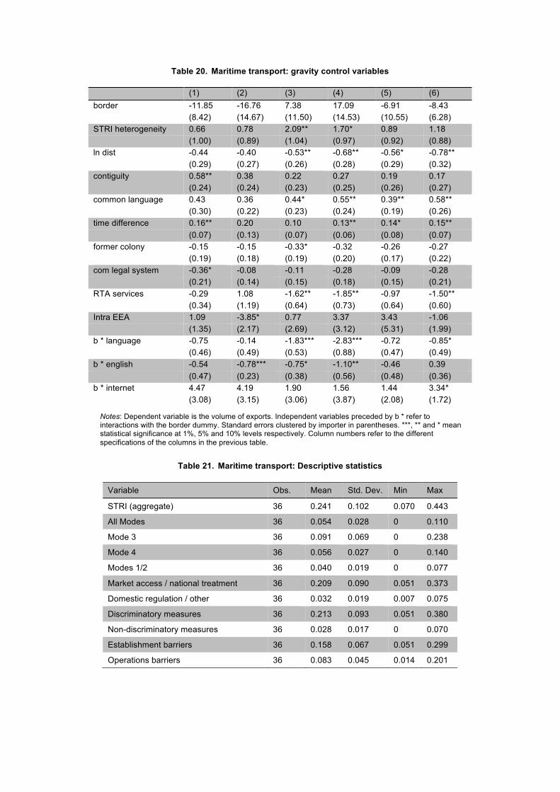
Table 20. Maritime transport: gravity control variables

(1) (2) (3) (4) (5) (6) border -11.85 -16.76 7.38 17.09 -6.91 -8.43 (8.42) (14.67) (11.50) (14.53) (10.55) (6.28) STRI heterogeneity 0.66 0.78 2.09** 1.70* 0.89 1.18 (1.00) (0.89) (1.04) (0.97) (0.92) (0.88) ln dist -0.44 -0.40 -0.53** -0.68** -0.56* -0.78** (0.29) (0.27) (0.26) (0.28) (0.29) (0.32) contiguity 0.58** 0.38 0.22 0.27 0.19 0.17 (0.24) (0.24) (0.23) (0.25) (0.26) (0.27) common language 0.43 0.36 0.44* 0.55** 0.39** 0.58** (0.30) (0.22) (0.23) (0.24) (0.19) (0.26) time difference 0.16** 0.20 0.10 0.13** 0.14* 0.15** (0.07) (0.13) (0.07) (0.06) (0.08) (0.07) former colony -0.15 -0.15 -0.33* -0.32 -0.26 -0.27 (0.19) (0.18) (0.19) (0.20) (0.17) (0.22) com legal system -0.36* -0.08 -0.11 -0.28 -0.09 -0.28 (0.21) (0.14) (0.15) (0.18) (0.15) (0.21) RTA services -0.29 1.08 -1.62** -1.85** -0.97 -1.50** (0.34) (1.19) (0.64) (0.73) (0.64) (0.60) Intra EEA 1.09 -3.85* 0.77 3.37 3.43 -1.06 (1.35) (2.17) (2.69) (3.12) (5.31) (1.99) b * language -0.75 -0.14 -1.83*** -2.83*** -0.72 -0.85* (0.46) (0.49) (0.53) (0.88) (0.47) (0.49) b * english -0.54 -0.78*** -0.75* -1.10** -0.46 0.39 (0.47) (0.23) (0.38) (0.56) (0.48) (0.36) b * internet 4.47 4.19 1.90 1.56 1.44 3.34* (3.08) (3.15) (3.06) (3.87) (2.08) (1.72)


Table 21. Maritime transport: Descriptive statistics


STRI (aggregate) 36 0.241 0.102 0.070 0.443

All Modes 36 0.054 0.028 0 0.110

Mode 3 36 0.091 0.069 0 0.238

Mode 4 36 0.056 0.027 0 0.140

Modes 1/2 36 0.040 0.019 0 0.077




Non-discriminatory measures 36 0.028 0.017 0 0.070



Table 22. Commercial banking: regression results

(1) (2) (3) (4) (5) (6) b * stri -55.49*** -471.36*** (12.32) (67.23) b * stri^2 98.79*** 290.97*** (31.76) (54.54) b * stri * lnGDP 17.44*** (1.92) b * stri * lnGDPpc 15.29*** (3.65) b * stri * lnDist -4.65* (2.46) b * DRO -60.15 (39.68) b * DRO^2 438.93 (338.75) b * MANT -79.09*** (10.61) b * MANT^2 271.30*** (38.87) b * DIS -97.61*** (13.88) b * DIS^2 426.48*** (74.48) b * NDIS 10.86 (33.21) b * NDIS^2 -294.21 (303.26) b * EST -168.31*** (24.74) b * EST^2 846.49*** (152.65) b * OPE 33.87** (16.17) b * OPE^2 -349.49*** (106.77) b * All Modes -1.59 (14.05) b * Mode 3 1.76 (8.42) b * Mode 4 -57.58*** (12.68) b * Modes 1/2 -65.69*** (11.27) Gravity Controls Yes Yes Yes Yes Yes Yes Intra EU Controls Yes Yes Yes Yes Yes Yes Exp * Year FE Yes Yes Yes Yes Yes Yes Imp * Year FE Yes Yes Yes Yes Yes Yes N 4238 4238 4238 4238 4238 4238


Table 23. Commercial banking: Intra EU control variables

(1) (2) (3) (4) (5) (6) b * stri 11.95 172.06** (18.64) (67.86) b * stri^2 -30.55 98.93 (62.54) (74.86) b * stri * lnGDP -2.10 (2.39) b * stri * lnGDPpc -12.74*** (3.93) b * stri * lnDist -2.67 (4.43) b * DRO 7.81 (29.34) b * DRO^2 159.37 (320.24) b * MANT -0.21 (18.51) b * MANT^2 22.51 (128.62) b * DIS 6.64 (15.96) b * DIS^2 -24.43 (97.46) b * NDIS -35.91 (25.98) b * NDIS^2 682.94** (303.30) b * EST 4.31 (20.13) b * EST^2 -53.66 (137.43) b * OPE -8.73 (16.69) b * OPE^2 270.79 (203.56) b * All Modes 6.55 (9.91) b * Mode 3 11.97 (10.68) b * Mode 4 28.35* (14.53) b * Modes 1/2 -3.89 (9.42) Gr. Controls Yes Yes Yes Yes Yes Yes Exp*Y FE Yes Yes Yes Yes Yes Yes Imp*Y FE Yes Yes Yes Yes Yes Yes N 4238 4238 4238 4238 4238 4238


Table 24. Commercial banking: gravity control variables

(1) (2) (3) (4) (5) (6) border -0.85 1.89 -0.18 -1.52 3.22 -7.38* (4.29) (4.00) (4.12) (4.41) (4.08) (4.46) STRI heterogeneity 1.72 -2.66** 0.45 -0.99 -0.50 -1.28 (1.44) (1.11) (1.24) (1.29) (1.03) (1.04) ln dist -0.95*** -1.10*** -1.24*** -1.32*** -1.28*** -1.47*** (0.12) (0.17) (0.12) (0.13) (0.12) (0.16) contiguity -0.02 -0.42* -0.12 -0.25 -0.10 -0.49** (0.28) (0.23) (0.23) (0.21) (0.20) (0.20) common language 1.17*** 0.65*** 0.64** 0.68*** 0.86*** 0.73*** (0.29) (0.20) (0.26) (0.23) (0.22) (0.20) time difference 0.08* 0.10* 0.11** 0.10** 0.09** 0.15*** (0.05) (0.06) (0.05) (0.05) (0.04) (0.06) former colony -0.45* -0.30** -0.56** -0.50** -0.33 -0.22 (0.25) (0.14) (0.26) (0.25) (0.20) (0.25) com legal system -0.09 0.20 0.26 0.22 0.01 0.24 (0.25) (0.15) (0.20) (0.19) (0.15) (0.16) RTA services -0.15 -0.19 -0.43 -0.39 -0.35 -0.48 (0.40) (0.29) (0.41) (0.41) (0.32) (0.29) Intra EEA -1.59 0.12 -1.28 -1.03 -0.50 -0.50 (1.43) (1.74) (1.23) (1.16) (1.16) (0.75) b * language -0.11 1.21*** -0.38 -0.57** -0.99*** -0.75*** (0.23) (0.17) (0.24) (0.25) (0.20) (0.16) b * english 1.44*** 1.58*** 1.98*** 2.11*** 2.26*** 2.17*** (0.17) (0.08) (0.19) (0.20) (0.19) (0.14) b * internet -0.38 -2.88*** -0.31 0.11 -0.21 1.33 (0.92) (0.85) (0.84) (0.95) (0.90) (0.96)


Table 25. Commercial banking: Descriptive statistics


STRI (aggregate) 42 0.189 0.122 0.064 0.551

All Modes 42 0.053 0.036 0 0.162 Mode 3 42 0.076 0.080 0.011 0.321 Mode 4 42 0.028 0.014 0 0.069 Modes 1/2 42 0.032 0.017 0 0.054







Services Trade Costs: Tariff equivalents of services trade...

Documents

Transcript of Services Trade Costs: Tariff equivalents of services trade...