Sequential, Multiple Assignment, Randomized Trials and Treatment Policies S.A. Murphy UAlberta,...

Sequential, Multiple Assignment, Randomized Trials

and Treatment Policies

S.A. Murphy

UAlberta, 09/28/12

2

Outline

• Treatment Policies

• Data Sources

• Q-Learning

• Confidence Intervals

3

Treatment Policies are individually tailored treatments, with treatment type and dosage changing according to patient outcomes. Operationalize sequential decisions in clinical practice.

k Stages for each individual

Observations available at jth stage

Action at jth stage (usually a treatment)

4

Example of a Treatment Policy

•Adaptive Drug Court Program for drug abusing offenders.

•Goal is to minimize recidivism and drug use.

•Marlowe et al. (2008, 2009, 2011)

5

non-responsiveAs-needed court hearings As-needed court hearings

low risk + standard counseling + ICM

non-complianthigh risk

non-responsiveBi-weekly court hearings Bi-weekly court hearings + standard counseling + ICM

non-compliant Court-determined disposition

Adaptive Drug Court Program

6

k=2 Stages

The treatment policy is a sequence of two decision rules:

Goal: Use a data set of n trajectories, each of the form

(a trajectory per subject) to construct a treatment policy. The treatment policy should produce maximal reward,

7

Why should a Machine Learning Researcher be interested in Treatment

Policies?

• The dimensionality of the data available for constructing decision rules accumulates at an exponential rate with the stage.

•Need both feature construction as well as feature selection.

8

Outline


• Data Sources

• Q-Learning


9

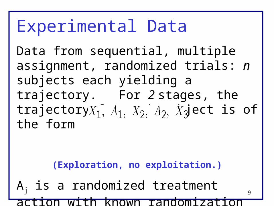
Experimental Data Data from sequential, multiple assignment, randomized trials: n subjects each yielding a trajectory. For 2 stages, the trajectory for each subject is of the form

(Exploration, no exploitation.)

Aj is a randomized treatment action with known randomization probability. Here binary actions with P[Aj=1]=P[Aj=-1]=.5

10

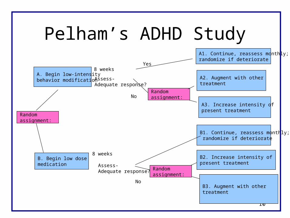
Pelham’s ADHD Study

B. Begin low dosemedication

8 weeks

Assess-Adequate response?

B1. Continue, reassess monthly; randomize if deteriorate

B2. Increase intensity of present treatment

Randomassignment:

B3. Augment with othertreatment

No

A. Begin low-intensity behavior modification

8 weeks


A1. Continue, reassess monthly;randomize if deteriorate

A2. Augment with other treatment

Randomassignment:

A3. Increase intensity of present treatment

Yes

No

Randomassignment:

11

Oslin’s ExTENd Study

Late Trigger forNonresponse

8 wks Response

TDM + Naltrexone

CBIRandomassignment:

CBI +Naltrexone

Nonresponse

Early Trigger for Nonresponse

Randomassignment:

Randomassignment:

Randomassignment:

Naltrexone

8 wks Response

Randomassignment:

CBI +Naltrexone

CBI

TDM + Naltrexone

Naltrexone

Nonresponse

Jones’ Study for Drug-Addicted Pregnant Women

rRBT

2 wks Response

rRBT

tRBTRandomassignment:

rRBT

Nonresponse

tRBT

Randomassignment:

Randomassignment:

Randomassignment:

aRBT

2 wks Response

Randomassignment:

eRBT

tRBT

tRBT

rRBT

Nonresponse

13

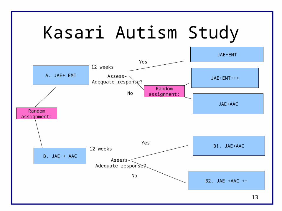
Kasari Autism Study

B. JAE + AAC

12 weeks


B!. JAE+AAC

B2. JAE +AAC ++No

A. JAE+ EMT

12 weeks


JAE+EMT

JAE+EMT+++

Randomassignment:

JAE+AAC

Yes

No

Randomassignment:

Yes

14

Newer Experimental Designs

• Using Smart phones to collect data, Xi’s, in real time and to provide treatments, Ai’s, in real time to n subjects. The treatments, Ai’s, are randomized among a feasible set of treatment options. – The number of treatment stages is very large—want

a Markovian property– Feature construction of states in Markov process

15

Observational data

• Longitudinal Studies

• Patient Registries

• Electronic Medical Record Data

16

Outline


• Data Sources

• Q-Learning/ Fitted Q-Iteration


17

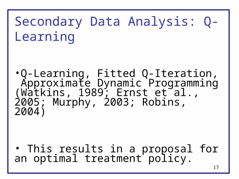
Secondary Data Analysis: Q-Learning

•Q-Learning, Fitted Q-Iteration, Approximate Dynamic Programming (Watkins, 1989; Ernst et al., 2005; Murphy, 2003; Robins, 2004)

• This results in a proposal for an optimal treatment policy.

•A subsequent randomized trial would evaluate the proposed treatment policy.

18

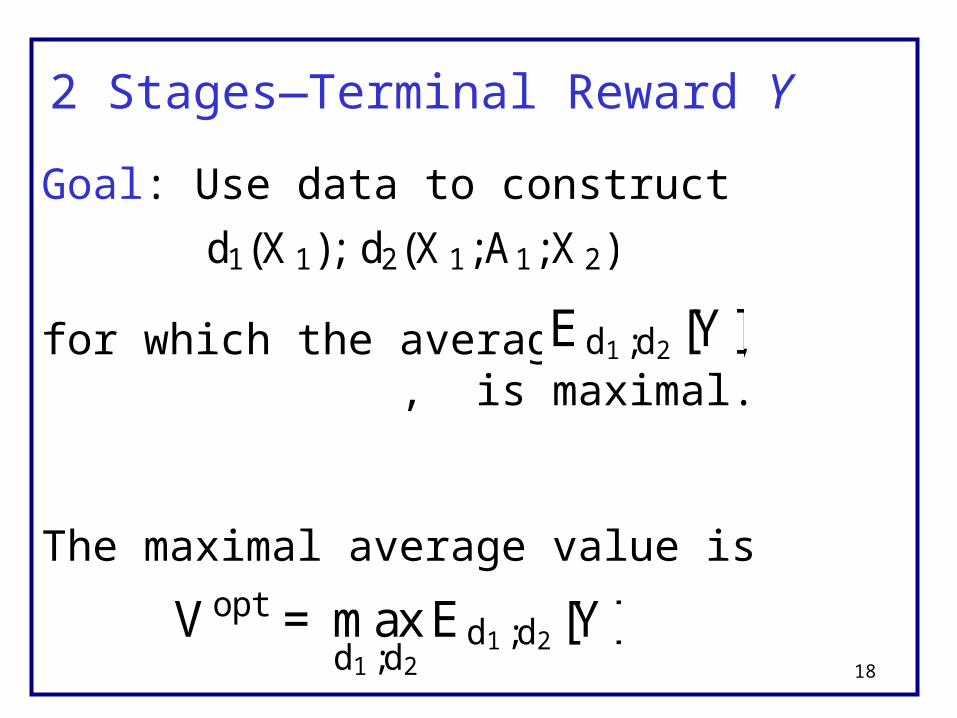
Goal: Use data to construct

for which the average value, , is maximal.

2 Stages—Terminal Reward Y

Ed1;d2 [Y ]

The maximal average value is

Vopt =maxd1 ;d2

Ed1 ;d2 [Y ]

d1(X 1); d2(X 1;A1;X 2)

19

Idea behind Q-Learning/Fitted Q

Vopt = E·maxa1

E·maxa2

E [Y jX 1;A1;X 2;A2 =a2]¯¯¯X̄ 1;A1 =a1

¸¸

² Stage2Q-function Q2(X 1;A1;X 2;A2) = E [Y jX 1;A1;X 2;A2]

Vopt = E·maxa1

E·maxa2

Q2(X 1;A1;X 2;a2)¯¯¯X̄ 1;A1 = a1

¸¸

² Stage1Q-function Q1(X 1;A1) = E·maxa2 Q2(X 1;A1;X 2;a2)

¯¯¯X̄ 1;A1

¸

Vopt = E·maxa1

Q1(X 1;a1)¸

20

Optimal Treatment Policy

The optimal treatment policy is

where

(d1; d2)

21

Use regression at each stage to approximate Q-function.

Simple Version of Fitted Q-iteration –

• Stage 2 regression: Regress Y on to obtain

• Arg-max over a2 yields

Q̂2 = ®̂T2S02+ ^̄T

2 S2a2

22

Value for subjects entering stage 2:

• is a predictor of

• is the dependent variable in the stage 1 regression for patients who moved to stage 2

maxa2 Q2(X 1;A1;X 2;a2)

23

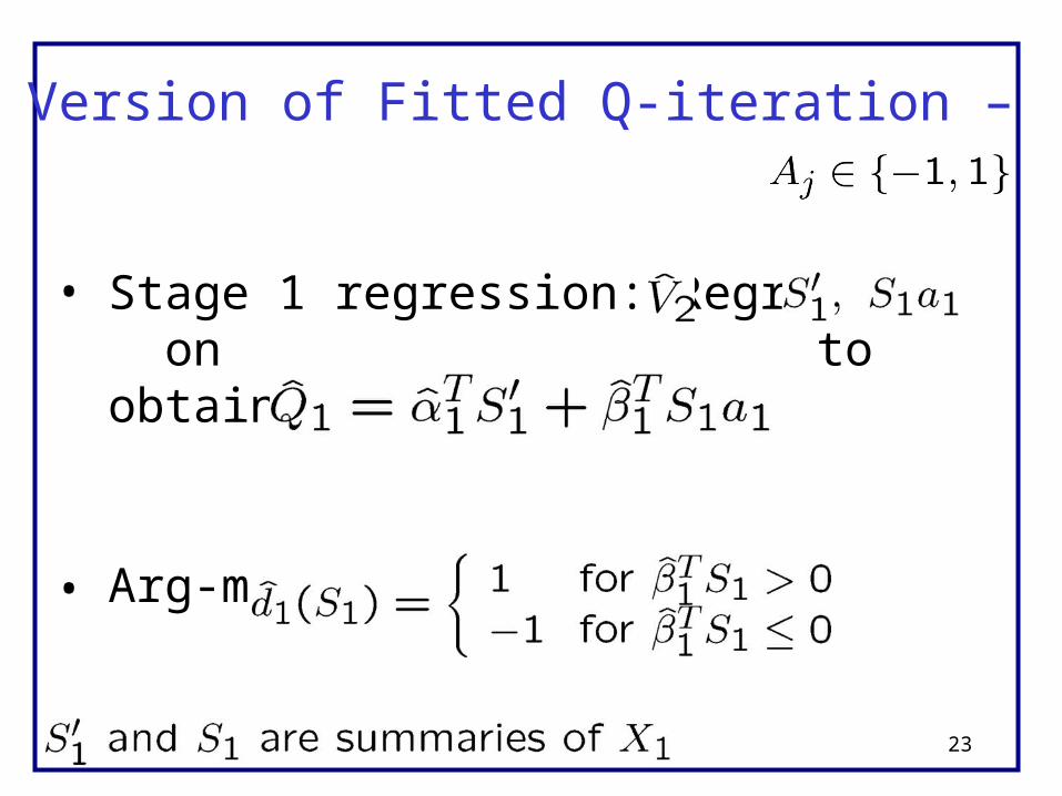
Simple Version of Fitted Q-iteration –

• Stage 1 regression: Regress on to obtain

• Arg-max over a1 yields

Decision Rules:

24

25

Pelham’s ADHD Study

B. Begin low dosemedication

8 weeks


B1. Continue, reassess monthly; randomize if deteriorate

B2. Increase intensity of present treatment

Randomassignment:

B3. Augment with othertreatment

No

A. Begin low-intensity behavior modification

8 weeks


A1. Continue, reassess monthly;randomize if deteriorate

A2. Augment with other treatment

Randomassignment:

A3. Increase intensity of present treatment

Yes

No

Randomassignment:

2626

138 trajectories of form: (X1, A1, R1, X2, A2, Y)

•X1 includes baseline school performance, Y0 , whether medicated in prior year (S1), ODD (O1)

– S1 =1 if medicated in prior year; =0, otherwise.

•R1=1 if responder; =0 if non-responder

•X2 includes the month of non-response, M2, and a measure of adherence in stage 1 (S2 )

– S2 =1 if adherent in stage 1; =0, if non-adherent

•Y = end of year school performance

ADHD

2727

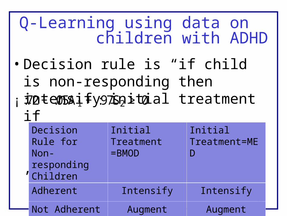
• Stage 2 regression for Y:

• Estimated decision rule is “ if child is non-responding then intensify initial treatment if , otherwise augment”

Q-Learning using data on children with ADHD

(1;Y0;S1;O1;A1;M2;S2)®2+A2(¯21+A1¯22+S2¯23)

¡ :72+ :05A1+:97S2 >0

2828

• Decision rule is “if child is non-responding then intensify initial treatment if . , otherwise augment”


¡ :72+ :05A1+:97S2 >0

Decision Rule for Non-responding Children

Initial Treatment =BMOD

Initial Treatment=MED

Adherent Intensify Intensify

Not Adherent Augment Augment

2929

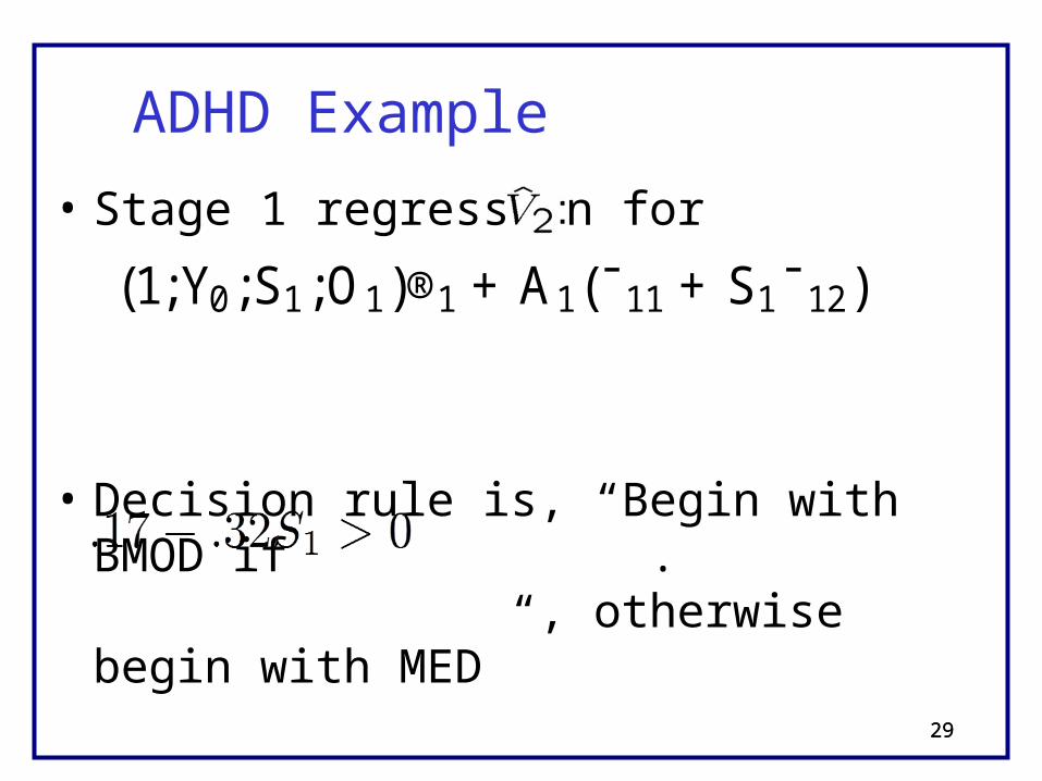
• Stage 1 regression for

• Decision rule is, “Begin with BMOD if . , otherwise begin with MED”

ADHD Example

(1;Y0;S1;O1)®1+A1(¯11+S1¯12)

3030

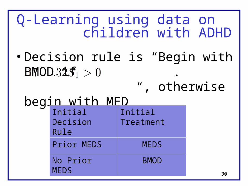
• Decision rule is “Begin with BMOD if . , otherwise begin with MED”


Initial Decision Rule

Initial Treatment

Prior MEDS MEDS

No Prior MEDS BMOD

3131

• The treatment policy is quite decisive. We developed this treatment policy using a trial on only 138 children. Is there sufficient evidence in the data to warrant this level of decisiveness??????

• Would a similar trial obtain similar results?

• There are strong opinions regarding how to treat ADHD.

• One solution –use confidence intervals.

ADHD Example

32

Outline


• Data Sources

• Q-Learning


3333

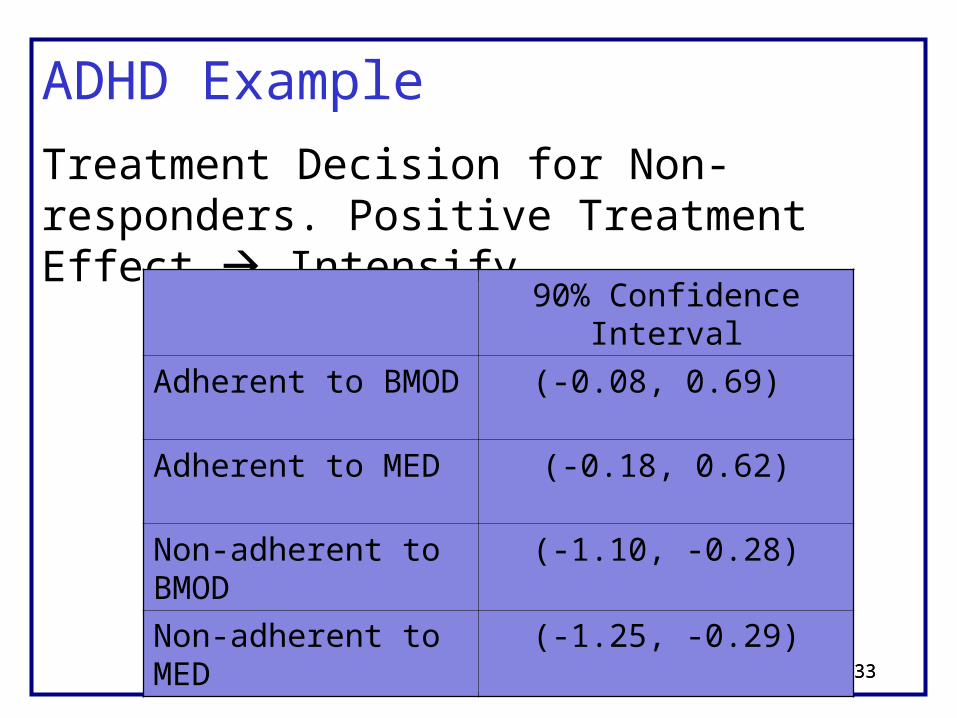
ADHD Example

Treatment Decision for Non-responders. Positive Treatment Effect Intensify

90% Confidence Interval

Adherent to BMOD (-0.08, 0.69)

Adherent to MED (-0.18, 0.62)

Non-adherent to BMOD (-1.10, -0.28)

Non-adherent to MED (-1.25, -0.29)

3434

ADHD Example

Initial Treatment Decision: Positive Treatment Effect BMOD

90% Confidence Interval

Prior MEDS (-0.48, 0.16)

No Prior MEDS (-0.05, 0.39)

3535

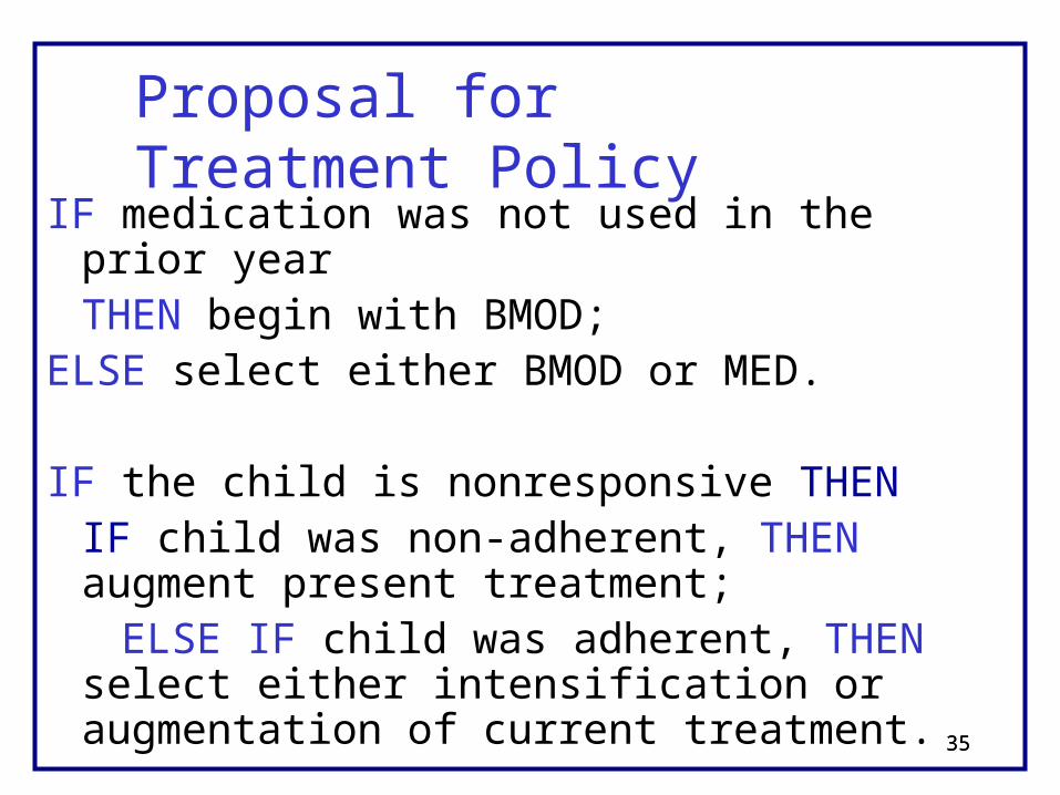
IF medication was not used in the prior year THEN begin with BMOD;

ELSE select either BMOD or MED.

IF the child is nonresponsive THENIF child was non-adherent, THEN augment present treatment;

ELSE IF child was adherent, THEN select either intensification or augmentation of current treatment.

Proposal for Treatment Policy

Constructing confidence intervals concerning treatment effects at stage 2 and stage 1.

The stage 2 is classical regression (at least if is low dimensional); constructing confidence intervals is standard.

Constructing confidence intervals for the treatment effects at stage 1 is challenging.

36

Confidence Intervals

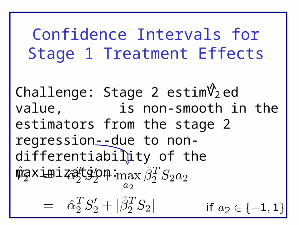
Challenge: Stage 2 estimated value, is non-smooth in the estimators from the stage 2 regression--due to non-differentiability of the maximization:

37

Confidence Intervals for Stage 1 Treatment Effects

V̂2

38

Non-regularity

• The estimated policy can change abruptly from training set to training set. Standard approximations used to construct confidence intervals perform poorly (Shao, 1994; Andrews, 2000).

• Problematic area in parameter space is around for which

• We combined a local generalization-type error bound with standard statistical confidence interval to produce a valid confidence interval.

P [̄ T2 S2 ¼0]> 0

39

Why is this non-smoothness, and the resulting inferential problems, relevant to high dimensional machine learning research?

•Sparsity assumptions in high dimensional data analysis

• Thresholding

• Nonsmoothness at important parameter values

40

Where are we going?......

• Increasing use of wearable computers (e.g smart phones, etc.) to both collect real time data and provide real time treatment.

• We are working on the clinical trial designs involving randomization (soft-max or epsilon-greedy choice of actions) so as to develop/ continually improve treatment policies.

• Need confidence measures for infinite horizon problems

41

This seminar can be found at:

http://www.stat.lsa.umich.edu/~samurphy/

seminars/UAlberta.09.28.12.pdf

This seminar is based on work with many collaborators, some of which are: L. Collins, E. Laber, M. Qian, D. Almirall, K. Lynch, J. McKay, D. Oslin, T. Ten Have, I. Nahum-Shani & B. Pelham. Email with questions or if you would like a copy:

[email protected]

Sequential, Multiple Assignment, Randomized Trials and Treatment Policies S.A. Murphy UAlberta,...

Documents

Transcript of Sequential, Multiple Assignment, Randomized Trials and Treatment Policies S.A. Murphy UAlberta,...