Sequential Entry and Strategic Deterrence in theAirline Industry

Federico CilibertoDepartment of EconomicsUniversity of Virginia

Preliminary Draft, March 2005Comments are Welcome.

Please Consider this Paper for the Young Economist Award.

Abstract

I extend the literature on entry in oligopoly markets (Bresnahan and Reiss[1990, 1991], Berry [1992], Mazzeo [2002], and Ciliberto and Tamer [2005])by determining endogenously whether firms play a simultanous or sequential-move game and whether firms deter new entrants. Moreover, when playing asequential game, firms are allowed to make ”deterrence investments” to preventnew entry (Bernheim [1984]). Using evidence from the US airline industrybetween 1996 and 2000, I find in preliminary results that incumbents do notsystematically deter new entrants in the airline industry.Keywords: Entry, Deterrence, Airline Industry, Repeated Game.JEL Classification: L12, L13

1 Introduction

I investigate the effect of firm strategic heterogeneity on market structure when firms

play repeatedly with each other. Previous empirical research assumes that firms

compete symmetrically with each other, but theories of entry show that incumbents

can accommodate some entrants but use predatory tactics with others.1 In particular,

I investigate whether major airline carriers (e.g. American) strategically deter new

entry of low cost carriers (e.g. Vanguard). Addressing this question has direct policy

implications because where entry is not artificially impeded, competition ensures1For example, see Bernheim [1984] or Dixit [1980].

1

that prices are in the long run reflective of the full cost of efficiently providing airlines

services.

To allow firms to deter new entrants, the type of game that airlines play is de-

termined endogenously. In particular, if there are no incumbents or if there is more

than one incumbent in the market, then the airlines play a simultaneous-move game.

If there is only one incumbent in the market then the airlines play a sequential-move

game.2 A critical difference between a sequential and a simultaneous-move game is

that in a sequential game firms can take actions to precommit themselves to aggres-

sive behavior towards their competitors. In particular, firms can make “deterrence

investments”, which include all investment that raise barriers to entry, and for which

incumbents must incur some investment costs (Bernheim [1984]).3

The first contribution of this paper is to extend the literature on entry in oligopoly

markets (Bresnahan and Reiss [1990, 1991], Berry [1992], Mazzeo [2002], and Ciliberto

and Tamer [2005]) by determining endogenously whether firms play a simultanous or

sequential-move game and whether firms deter new entrants. Bresnahan and Reiss

[1990] and Berry [1992] considered a sequential and a simultaneous-move game as al-

ternatives to describe the interaction between car dealers and airlines. However, since

they used a cross-section of data, Bresnahan and Reiss and Berry exogenously de-

termined whether firms were playing a simultaneous or sequential-move game. Here,

the selection of the type of game played is endogenous.

The second contribution of this paper is to propose a way to determine whether

incumbents strategically deter new entrants. To identify deterrence investments,

I use changes over time in firms’ entry decisions. The idea is to compare entry

decisions across similar markets whose market structures change differently over time.

In particular, if there are two markets that have identical observable and unobservable

characteristics, and in one there is only one incumbent over time, while in the other2As will be shown in the analysis of the data, the only reasonable empirical hypothesis is that

deterrence only occurs when there is only one incumbent in a market.3For example, the monopolist can build excess production capacity as a threat against new

entrants. As Bernheim explains, the definition of deterrence investment is intentionally ambiguousto abstract from the complex issues that arise with particular theories of entry deterrence, and itincludes any barrier that an incumbent raises to prevent entry, and for which the incumbent mustpay some investment costs. There are several theories of strategic investment, for example Bulow,Geanakoplos, and Klemperer [1985], Fudenber and Tirole [1984], Dixit [1980], Schmalensee [1981,1978], Gelman and Salop [1983], Fudenberg and Tirole [1983], Judd [1985].

2

there periods with two firms, then it must be the case that the incumbent in the first

market can deter new entrants. Using this simple idea, I can estimate the costs that

incumbents must face to make “deterrence investments,” and determine if there are

some airlines that systematically prevent new entry.

To allow for the type of game played by airlines to be determined endogenously,

I use the methodology developed by Ciliberto and Tamer [2005]. This methodol-

ogy allows multiple equilibria in the number and identity of firms when firms play

a simultaneous-move entry game. Multiple equilibria in the number and identity

of firms can also exist in a sequential-move game with more than two players since

all firms except the incumbent play a simultaneous-move subgame.The methodology

developed by Ciliberto and Tamer allows to make inferences on a “class of models”

rather than looking for assumptions that pin down a unique model. The estimation

strategy is thus directed at a class of models that obey the fundamental equilibrium

condition that if a firm enters into a market then it expects to make nonnegative prof-

its. This fundamental condition provides a set of inequality restrictions on regressions

that restrict the parameters to a set. Thus, the object of interest is in general a set of

parameters of the profit functions that correspond to models with different consistent

equilibrium selection rules.

I use panel data from the US airline industry between 1996 and 2000 and inves-

tigate competition between major airlines (e.g. American) and low cost carriers (e.g.

Vanguard), with a special focus on their interaction in markets to and from the major

airlines’ hubs (e.g. Dallas Fort Worth). To identify the ability of the major firms to

deter low cost carriers to enter into profitable markets from other barriers to entry

that low cost carriers face, I collected original data on institutional restrictions that

low cost carriers face at several airports in the largest metropolitan statistical areas

in the United States.

2 The Entry Game Played by the Airlines

The game played by the airlines is here assumed to be a static game that is repeatedly

played over time, with time being denoted by t = 1, ..., T . Airlines are assumed to

know each other strategies and payoffs, thus this is a complete information game.

3

Airlines must decide whether or not to enter into a market. There are I airlines,

indexed by i = 1, ..., I, that must decide whether to enter into market m = 1, ...,M

at time t = 1, ..., T . Let yimt = 1 if the firm i enters in market m at time t and

yimt = 0 otherwise. Let πimt (ymt) denote the profit made by firm i in market m at

time t. Finally, let ymt = (y1mt, ..., yIm t) denote the vector of firms’ strategies.

I consider two types of games, a one-shot game and a sequential-move game. In

a simultaneous-move game firms choose their actions without observing the other

firms’ actions. In a sequential-move game, at least one firm choose her action before

the other firms choose theirs, and all other firms can observe the first mover’s choice.

Thus, in a sequential-move game the followers’ actions are conditional on the first

mover’s actions.

I consider the subgame-perfect Nash equilibrium concept to solve the game that

airlines play. A subgame-perfect Nash equilibrium is a combination of firm’s strate-

gies y∗mt = (y∗1mt, ..., y

∗Im t) such that no firm can unilaterally benefit from choosing a

different strategy at any stage of the game. In an entry game at a Nash equilibrium

y∗mt = (y∗1mt, ..., y∗Im t) every firm that enters must make a nonnegative profit, while

firms that do not enter expect to make a negative profit should they decide to enter:

πimt (y∗mt) ≥ 0⇔ y∗imt = 1.

At each period, the entry game is either a simultaneous entry game or a sequential

entry game. Airlines play a simultaneous-move game in market m if at time t there

is no incumbent in the market, that is if the market was not served by any airline at

time t− 1. Airlines play a sequential-move entry game at time t in market m if one

airline was present at time t− 1 in the market.

Whether airlines play a simultaneous or sequential-move game is determined en-

dogenously. To see why, consider Table 1, which presents several possible scenarios

with three airlines (American, Delta, United) in one particular market. In the first

quarter of 1998 none of the three airlines was serving this particular market. There-

fore, in the second quarter of 1998, there was no incumbent, and thus the three airlines

played a simultaneous-move game. Among the possible equilibria, the airlines ended

up in the one where American entered into the market, while Delta and United did

4

not enter. In the third quarter of 1998, American is now the incumbent and moves

first. Delta and United follow. The interpretation of the game in the other quarters

is analogous.

[TABLE 1 APPROXIMATELY HERE]

Consider now the game played in the second quarter of 1998 by the three firms.

American is the incumbent and thus American must decide whether or not to enter

before Delta and United take their decisions. Figure 1 shows two games, one where

American cannot deter new entrants (the upper game), and one where American can

make ”deterrence investments” to prevent new entry in the market (the lower game).

[FIGURE 1 APPROXIMATELY HERE]

Consider first the game where American cannot deter new entry, which is Figure

1a. American can decide whether to enter or not, and then Delta and United play

a simultaneous move against each other after observing American’s decision. To

determine the one-shot equilibrium of the game, the game is solved through backward

induction. First we determine the Nash pure strategy equilibria in the last stage of

the game, the one played by Delta and United, for any given entry decision made by

American. Then, we determine the optimal choice of American. For the equilibrium

to be subgame perfect, American will enter if in any of the equilibria in the last stage

of the game American makes nonnegative profits.

Consider, for example, the situation where there are two equilibria in the simultaneous-

move game, which is the game that the three firms would be playing if American did

not have a first-mover advantage. Let the first equilibrium be (yAA, yDL, yUA) =

(0, 1, 1): American does not enter, while both Delta and United enter into the mar-

ket. Let the second equilibrium of the last stage game be (yAA, yDL, yUA) = (1, 0, 1):

American enters, Delta does not enter, United enters. In the sequential game where

American moves first, there will be a unique equilibrium, (yAA, yDL, yUA) = (1, 0, 1).

Generally, the fact that American moves first does not imply that there exists

a subgame perfect equilibrium where American is in the market. However, this is

where the role of deterrence comes to play. Following Bernehim [1984], I will assume

5

that an incumbent can opt to deter new entrants when the game is sequential. An

incumbent firm i can make deterrence investments by paying a deterrence cost ci at

time t and ensure that it will be a monopolist at time t+ 1.

To understand the role of the deterrence investments, consider again the exam-

ple of the strategic interaction between American, Delta, and United illustrated in

Table 1. Figure 1b presents the game with deterrence. In the third quarter of

1998, American must decide first whether to deter new entrants. If American pays a

deterrence cost cAA, then American can deter new entrants and make the monopoly

profit πMAA minus the deterrence cost. If American does not pay the deterrence cost,

then the airlines play the sequential game illustrated in Figure 1a.

American will deter new entrant if the cost of deterrence is lower than the monopoly

profit and if the profit that American makes under deterrence, πMAA − cAA, is notsmaller than the lowest profit that American would make in any of the subgame per-

fect equilibria of the sequential game played by airlines should American not deter

new entrants (the game in Figure 1a). Therefore, American will not always deter

new entrants even when she can do so.

Whether airlines play a simultaneous-move game, a sequential-move game, or a

sequential-move game with deterrence is determined endogenously in this framework.

The objective of this paper is to show that we can use repeated observations over

time across markets to identify whether firms are able to deter new entrants.

3 Identification of Strategic Deterrence

There are several reasons why we only observe one firm for a long period of time in a

market that are completely unrelated to strategic deterrence. First, there might only

be space for one firm in the market, in the sense that two firms would not be able to

make nonnegative profits. Second, there might be multiple equilibria with different

number of firms in a market, and we might simply observe the equilibrium with one

firm rather than one with two or more firms.

The fundamental question is then how to identify from the revealed actions of the

airlines whether in the data there is one firm because the incumbent deters new entry

or because of other reasons unrelated to strategic deterrence.

6

The first two columns of Table 2 illustrate how to identify strategic deterrence.

There are two firms that compete against each other in one market, and for simplicity

of exposition I consider American and Delta as the two competing firms. At time 0

neither firm is present in the market, because neither firm makes nonnegative profits.

Then at time 1 there is a positive shock and either one but not both of the two firms

can enter into the market. American enters. At time 2 there is another positive shock

and both American and Delta can enter into the market. However, we observe only

American in the market. At time 3 there is a negative shock and American must exit

the market. At time 4 there is a positive shock and either one but not both of the two

firms can enter into the market. This time Delta enters. At time 5 there is another

positive shock and both American and Delta enter into the market.

The first two columns of Table 2 show that American was able to prevent the

entry of Delta when American was the incumbent, while Delta was not able to prevent

the entry of American when Detla was the incumbent.

[TABLE 2 APPROXIMATELY HERE]

The type of evidence provided in Table 2 implies that American must face lower

deterrence costs than Delta and that American did deter Delta from entry at time

t=2. The last column of Table 2 shows how the identification strategy discussed in

the first two columns of Table 2 can be used to identify the cost that airlines must

incur to deter new entrants. Since American deterred Delta from entry at time t=2,

then it must be that πMAA − cAA > πDAA, that is the profits that American makes in

this market when it deters Delta are higher than the profits that it would make as a

duopolist. On the contrary, πMDL − cDL > πDDL, the profits that Delta would make as

a monopolist in this market are not large enough to justify the deterrence costs.

The variation across and within markets identifies πMAA, πDAA, π

MDL, π

DDL, cAA, and

cDL. In a static model it is possible to identify only πMi and πDi from the variation

across markets in the number (and identity) of firms. Clearly it is possible to identify

deterrence only in a repeated static game because of the variation in the number and

identity of firms over time across and within identical markets.

The critical feature of this stylized model is that the incumbent faces a trade-

off. The incumbent can deter new entrants, but only at a cost ci. Whether the

7

incumbent will actually deter new entrants will depend on the characteristics (and

unobservables) of the market and of the new entrant.

4 Econometric Model

4.1 Basic Methodology

The estimation methodology adapts Ciliberto and Tamer [2005] to a panel dataset.

Consider a k-player binary game where the strategy of player i is yi = 1 or 0

depending on whether the i’s profit crosses a threshold. For player i, this can be

written as

yi = 1 if Πi(xi,y−i, θ, ²i) ≥ 0

where y−i is the k − 1 binary zero-one vector of other players’ strategies, xi is avector of regressors, and ²i is the part of player i’s utility that is unobserved by

the econometrician.4 yi and y−i are observed, while the profits, Πi and Π−i, are

unobservable.

The observed part of profit Π() is known up to the finite dimensional parameter

θ and the unobserved part of the profit function (the ²’s) is independent of x. ²

is known to the players but unobserved to the econometrician, thus this is a game

of complete information. The data consist of a random iid sample of observations

(markets) (yi,xi) for i = 1, . . . , N . In addition, ² = (²1, . . . , ²k) is a mean zero random

variable, independent of x, and has a known (up to a finite dimensional parameter

Ω) distribution FΩ.

I consider panel data, and thus there should be a strong correlation over time in

the unobservables that determine firms’ decisions. New entrants might never enter

into a market because the market is always unprofitable for two firms. The econo-

metric analysis allows for the market unobservables to be constant over time. Firms’

unobservables are also correlated over time, and low cost carriers might never enter

because they suffer bad shocks in that market.

I write the unobservable error ²imt as follows:4For simplicity, there are no market and time specific subscripts in this section.

8

²imt = νm + ξmt + ηim + ζ imt.

νm represents market unobservables that are constant over time to capture, for

example, the fact that in market m there is a large share of business passengers.

ξmt is a market shock that changes over time, and which affects firms in the same

way, for example changes in the demand for travel over time. ηim is a time invariant

market specific airline shock, to allow different firms to face different unobservables

in the same market, for example some airlines might see a larger share of business

passengers in the same market than other airlines do. Finally, ζimt are time variant

firm specific shocks.

The model provides the following inequality restrictions on regressions:

H1(x, θ) ≤ Pr(y|x) ≤ H2(x, θ)

where Pr(y|x) is a 2k vector of of choice probabilities that can be consistently esti-mated using the data and the inequalities are interpreted element by element. The

H’s are functions of θ and the distribution function FΩ where Ω is part of the vector

θ. Heuristically, the identified set, ΘI , is the set of parameter values that obey these

restrictions for all x almost everywhere and represents the set of economic models

that is consistent with the empirical evidence. For a given parameter value, the esti-

mator is based on minimizing the distance between this vector of choice probabilities

and the set of predicted probabilities. On the set ΘI , this distance is minimized.

The estimator is a sharp two step minimum distance estimator: in the first step the

conditional choice probabilities are estimated non-parametrically, and in the second

stage the estimates of the set ΘI are obtained. This sharp set contains all the possible

parameter values that are consistent with the set of economic models that obey our

fundamental assumption. In general games, it is not possible to derive these functions

analytically since that would entail solving for the equilibria of the game, a task that

can be very complicated. To obtain an estimate of these functions for a given x and

a given parameter value, a simulation procedure is provided in Ciliberto and Tamer

[2005]. I will simulate random draws of νm, ξmt, ηim, and ζimt from four independent

normal distributions with mean zero and variance equal to 1.

9

4.2 Specification

I assume the following profit function for firm i = 1, ..., I in market m = 1, ...,M at

time t = 1, ..., T ::

π∗imt ' αi0 + αiXmt + βiZimt +Xj 6=i

δijyjmt + ²imt.

where Xmt are exogenous determinants of profits. ²imt is the part of firms’ profits

that cannot measured but that firms observe and act on. Zimt is the measure of

observable heterogeneity for the airlines. The parameters δij measure the effect that

the presence of one of the other airlines has on the probability of observing firm i in the

same market. For example, the parameters δii could measure a particular aggressive

behavior of one airline (e.g. American) against another airline (e.g. Southwest). δij

captures the effect that the entry by airline j has on i’s unobserved profits. In this

way, the analysis captures the possibility that the firms’ profits might change with the

number and identity of entrants. Here, θ = (α0,αX ,β, δ), where α0 is a I×1 vectorof parameters; αX is I × k matrix of parameters (with k exogenous determinants ofdemand); β is a I × 1 vector of parameters; δ is matrix of I × I parameters.

The empirical specifications consider the competition between airline alliances.

In particular, the first airline alliance is made of American Airlines and TWA. If

American or TWA is in the market, then yAA = 1, otherwise yAA = 0. The second

airline alliance is the Star Alliance, and is made of United and USAir, and is indexed

by ySA = 1 if one of these two firms is in the market; the third airline alliance is Sky

Team, and is made of Continental, Delta, and Northwest, and is indexed by ySK = 1

if one of these three firms is in the market; then there is Southwest, indexed by yWN .

Finally, there is an indicator variable yLCC = 1 if at least one of the other low cost

carriers is in the market. Let Υ = AA,SA, SK,WN,LCC.

4.2.1 Statistical Model 1: Firms Play A Simultanous-Move Game

When airlines play a simultaneous-move game I estimate the following statistical

model, which I call Statistical Model 1:

10

yi,mt = 1

⎡⎣πSIMimt = αi0 + αiXXmt + βiZi,mt +X

j∈Υ/i

δijyj,mt + ²i,mt ≥ 0

⎤⎦ , i ∈ Υ. (1)

This is the most general specification of a simultaneous-move game. πSIMimt is the

profit made in the simultaneous move game. Each firm has a different effect on

the competitors’ entry decision. For example, the effect of American’s presence on

Southwest is given by δWNAA and on the members of the Sky Team (e.g. Delta) is given

by δSKAA . The dummies introduce a measure of heterogeneity, as they capture how

each firm affects the entry decision of the other firms. Second, observe that we can

also allow for heterogeneous effects of market presence. For example, βAA measures

the effect that American’s market presence has on American’s decision to enter. The

model also here allows for multiple equilibria in the number of firms.

4.2.2 Statistical Model 2: Firms Play A Sequential-Move Game

Consider now the case when one firm, say firm h, was the only firm in the market at

time t − 1. Then firm h has a first-mover advantage. I consider first the case when

firm h cannot make deterrence investments (possibly because they are prohibitively

expensive).

The statistical model for a sequential-move game is complicated to write, because

firm h can move first and because the equilibrium must be subgame perfect. If

there is at least one subgame perfect pure strategy equilibrium where firm h makes

nonnegative profits, then the statistical model (Statistical Model 2) is given as

follows:

⎧⎪⎨⎪⎩yi,m = 1

hπSEQimt = αi0 + αiXXmt + βiZi,mt + δih +

Pj∈Υ/i,h δ

ijyj,mt + ²i,mt ≥ 0

iconditional on πSEQhmt = αh0 + αhXXmt + βhZh,mt +

Pj∈Υ/h δ

hj yj,mt + ²h,mt ≥ 0,

i ∈ Υ/ h .(2)

Otherwise, if there is no subgame perfect equilibrium with h in the market, the

statistical model is given by:

11

⎧⎪⎨⎪⎩yi,m = 1

hπSEQimt = αi0 + αiXXmt + βiZi,mt +

Pj∈Υ/i,h δ

ijyj,mt + ²i,mt ≥ 0

iconditional on πSEQhmt = αh0 + αhXXmt + βhZh,mt +

Pj∈Υ/h δ

hj yj,mt + ²h,mt < 0,

i ∈ Υ/ h .

4.2.3 Statistical Model 3: Firms Play A Sequential-Move Game withDeterrence

Finally, firms might decide to make deterrence investments when they have a first-

mover advantage. Consider again the case where firm h moves first, but now firm h

can make deterrence investments.

The statistical model is even more complicated now because the first mover must

decide whether to make the deterrence investments or not. If there is a subgame

perfect equilibrium where firm h makes nonnegative profits and where the profits

are larger than those that firm h would make with deterrence investments then, the

Statistical Model 3 is written as:

⎧⎪⎪⎨⎪⎪⎩yi,m = 1

hπSEQimt = αi0 + αiXXmt + βiZi,mt + δih +

Pj∈Υ/i,h δ

ijyj,mt + ²i,mt ≥ 0

iconditional on:

(πSEQhmt = αh0 + αhXXmt + βhZh,mt +

Pj∈Υ/h δ

hj yj,mt + ²h,mt ≥ 0,

and πSEQhmt ≥ πDEThmt = αh0 + αhXXmt + βhZh,mt − ch + ²h,mt.(3)

If, however, firm h, the first mover, makes higher profits when it deters new

entrants, then the statistical model is given as follows:½yi,m = 1

£πDEThmt = αh0 + αhXXmt + βhZh,mt − ch + ²h,mt ≥ 0

¤yi,m = 0 for i ∈ Υ/ h ,

conditional on πDEThmt > πSEQhmt .

12

5 Data

5.1 Ticket and Passenger Trip Data

Fare and passenger data are from the Origin and Destination Survey (DB1B), which

is a 10 percent sample of airline tickets from reporting carriers.5 These are quarterly

data from the first quarter in 1996 to the third quarter in 2000. The data are organized

by market and carrier.

A market is defined as a trip between two airports, regardless of origin and des-

tination, and regardless of connections. For example, a trip from Atlanta (ATL) to

Miami (MIA) and a trip from Miami to Atlanta are considered as trips in the same

market ATLMIA, regardless of the whether the trip was on nonstop, direct, or con-

necting flights. Trips from the same city but different airports are treated as different

markets. Therefore, the market between Atlanta and Chicago O’Hare, ATLORD, is

different from the market between Atlanta and Chicago Midway, ATLMDW . The

dataset includes markets between the airports of the largest 50 metropolitan statis-

tical areas in terms of population. There are 422markets.6

There are 8018 market-year-quarter observations. Table 3 reports the summary

statistics for the variables used in the analysis.

As discussed when presenting the econometric model, there are five players in this

game, which correspond to the three alliances, Southwest and a type called Low Cost

Carriers. The members of the three alliances are given in Table 3, which provides

summary statistics by the quartiles of the size of the market.7 Market size is measured

by the log of the product of the population at the endpoints (Berry [1992]). In this

table I have split the market size in 4 quartiles (large, medium large, medium small

and small).

[TABLE 3 APPROXIMATELY HERE]5The details of how to construct the data used in this paper are given in Ciliberto [2005], and

Ciliberto and Tamer [2005].6Because of the computational burden associated with the methodology used in this paper, I

draw a random sample with replacement of 500 markets to limit the number of markets.7Any carrier that is independently owned is included in the dataset, even if it serves as a regional

carrier of one of the major airlines in one market.

13

The first row shows summary statistics for the variable AA, which is equal to 1 if

either American or TWA are in the market. We observe that American or TWA serve

half of the market-year-quarter observations in the sample. This percentage does not

change by market size. The interpretation is analogous for the rows Star Alliance,

Sky Team, Southwest, and LCC.

The second set of variables are the measures of firm heterogeneity, which is equal

to the percentage of the total markets out of an airport that an alliance serves. In

particular, this percentage is calculated as the fraction of the average across airports

and across members of an alliance, divided by the total number of markets that are

served in a given quarter and in a given year from the end point airports. Notice that

firm heterogeneity does not vary by market size.

The last four rows of Table 3 show the summary statistics for the exogenous

determinants of profits. The first exogenous characteristics is income, which is com-

puted as the log of the average of the average personal income at the endpoints.

Markets of different size do not differ by income.8 Then I present the nonstop market

distance between the endpoints, which does not differ across markets of different sizes.

Tourist is a categorical variable that takes a value equal to 1 if the market involves

an airport in either Florida or California. Smaller markets are less likely to be tourist

markets. HubMarket is a variable that is equal to 1 if one of the endpoints is the hub

of one of the major airlines.9 Small markets are less likely to involve a hub airport.

Table 4 presents the distribution of these five types of firms across markets of

different sizes.

[TABLE 4 APPROXIMATELY HERE]

The table suggess that there is no clear relationship between market size and

number of firms in a market (Ciliberto and Tamer [2005]). This suggests that multiple

equilibria in the number and identity of firms exist.8The continuous variables presented in Table 3 are discretized in quartiles in the empirical analy-

sis.9Following Borenstein [1990], hub airports are Chicago O’Hare (American Airlines and United

Airlines); Dallas Forth-Worth (American Airlines); Houston International (Continental); Phoenix(America West); Detroit and Minneapolis/St. Paul (Northwest); St. Luois (TWA); Charlotte andPittsburgh (USAir); Denver (United Airlines); Atlanta (Delta Airlines).

14

The critical variation that is needed for the econometric analysis concerns entry

and exit from airline markets. In order to identify the role of strategic deterrence it is

crucial to see firms entering in markets that were not previously served by any airline

and firms entering in markets that are already served by other airlines.This variation

in the market structure within markets over time is crucial to identify the effect of

strategic deterrence on market structure from the role that sunk costs, operating

costs, and demand changes have on market structure.

Table 5 illustrates this type of variation in the data.

[TABLE 5 APPROXIMATELY HERE]

There are 1217 new entries over the time period. Some patterns are clear from

the table. First, 40 percent (489 out of 1217) of these new entries occur where there

is more than one incumbent in the market. Second, there is half as much entry where

a Low Cost Carrier is the only incumbent in the market than where one of the three

major alliances is in the market. There is even less entry where Southwest is the only

incumbent in the market. Finally, Southwest enters disproportionately in markets

where there is more than one incumbent.

In light of the discussion of Section 3, Table 5 provides a useful set of stylized

facts that should serve as a roadmap for the econometric analysis. Table 5 suggests

that incumbents generally might be able to deter new entry, and that Southwest

in particular is able to deter new competitors. Naturally, these are simple cross

tabulations which do not control for market characteristics.

5.2 Institutional Barriers to Entry

A critical set of market characteristics that might determine the entry patterns de-

scribed in Table 5 are institutional barriers to entry. In an extensive analysis of

airline competition, the United States General Accounting Office reported in 1990

the results of surveys among airport administrators and travel agents on industry

practices that limited entry in the airline industry (GAO [1989, 1990, 1990b, 1996]).

The survey found that limited access to airport facilities acted as barriers to entry.

As a result of the governmental, public and academic concern with the existence

of barriers to entry in the airline markets, on April 5, 2000, President Clinton signed

15

the Wendell H. Ford Aviation Investment and Reform Act for the 21st Century (AIR

21) into law. AIR 21 identified a set of “major airports” that had to be available on a

reasonable basis to all carriers wishing to serve these airports. AIR 21 provided that

beginning in fiscal year 2001, no passenger facility fee could be charged by a “major

airport” and no federal grant could be made to fund an airport unless the airport had

submitted a written competition plan. The competition plan had to include informa-

tion on the availability of airport gates and related facilities, leasing and sub-leasing

arrangements, gate-use requirements, patterns of air service, gate-assignment policy,

financial constraints, airport controls over air- and ground-side capacity, whether the

airport intends to build or acquire gates that would be used as common facilities, and

airfare levels (as compiled by the Department of Transportation) compared to other

large airports.10

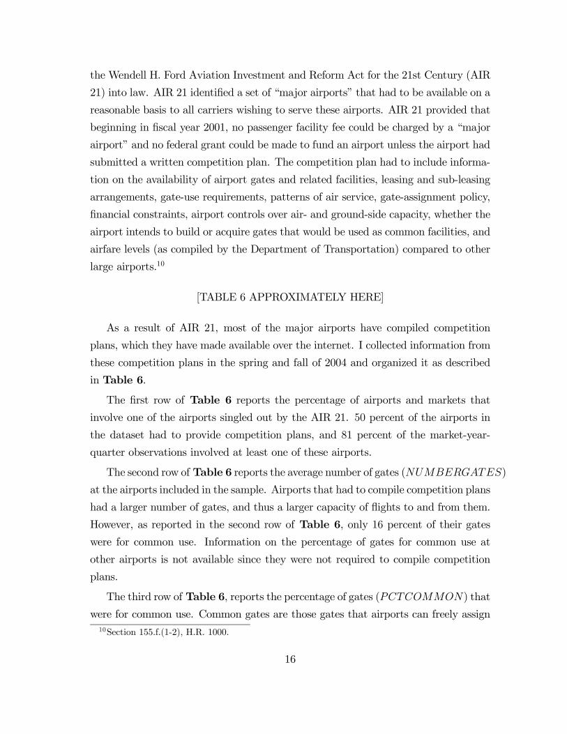
[TABLE 6 APPROXIMATELY HERE]

As a result of AIR 21, most of the major airports have compiled competition

plans, which they have made available over the internet. I collected information from

these competition plans in the spring and fall of 2004 and organized it as described

in Table 6.

The first row of Table 6 reports the percentage of airports and markets that

involve one of the airports singled out by the AIR 21. 50 percent of the airports in

the dataset had to provide competition plans, and 81 percent of the market-year-

quarter observations involved at least one of these airports.

The second row of Table 6 reports the average number of gates (NUMBERGATES)

at the airports included in the sample. Airports that had to compile competition plans

had a larger number of gates, and thus a larger capacity of flights to and from them.

However, as reported in the second row of Table 6, only 16 percent of their gates

were for common use. Information on the percentage of gates for common use at

other airports is not available since they were not required to compile competition

plans.

The third row of Table 6, reports the percentage of gates (PCTCOMMON) that

were for common use. Common gates are those gates that airports can freely assign10Section 155.f.(1-2), H.R. 1000.

16

to airlines. Other gates are leased on a preferential or exclusive base. The higher

the percentage of gates that are common, the easier should be for new entrants to

enter into a market. Only 16 percent of the gates were for common use. The data do

not show any type of relationship between the number of firms and the percentage

of gates that are common. This variable is discretized in quartiles in the empirical

analysis.

Airlines can sublease their gates to other airlines. The fourth row of Table 6

shows the summary statistics for the variable LIMIT , which is equal to 1 if airlines

can sublease gates but they cannot charge fees in excess to limits established by

airports. In 58 percent of the airports identified by the AIR 21, the airport had

introduced a limit to the sublease fees that could be charged by the airlines. Notice

that only 10 percent of the markets involved an airport that had introduced limit on

the sublease fees.

The fifth row shows the summary statistics for the variable ADMINLIMIT ,

which is the actual limit on sublease fees when a limit exists. In the empirical analysis,

ADMINILIMIT is a categorical variable equal to 1 if the sublease fee is larger than

100 percent. Among the airports that imposed limits on sublease fees, 68 percent of

them imposed limits larger than 100 percent.

The sixth row of Table 6 shows the summary statistics for the categorical variable

MII, which is equal to 1 if the airport has a Majority-in-Interest Agreement with

any of the airlines at the airport. It turns out that most of the airports identified by

the AIR 21 did have an MII in place.

6 Empirical Analysis

The empirical analysis develops specifications that are increasingly general. All spec-

ifications allow for firm strategic heterogeneity. However, to show the effect of adding

control variables I will start with simpler specifications where the models do not in-

clude observable firm heterogeneity and do not include institutional barriers to entry.

17

6.1 Baseline Specifications

Table 7 presents the results of the estimation of Statistical Models 1, 2, and 2 when

I do not include firm heterogeneity and measures of institutional barriers to entry.

[TABLE 7 APPROXIMATELY HERE]

The first column of Table 7 presents the coefficient bounds for the Statistical

Model 1. In this Table, the effect of one firm, say American, on the other firms, SA,

SK, WN , and LCC is the same. Therefore δAADL = δAAWN , for example. I estimate the

effect of American on the other airlines to be included in [−4.160,−3.551]. The effectis negative, as expected: American’s presence in the market reduces the probability

that we observe one of the other four airlines in the market. The results are similar for

the other firms. The effect of United or USAir (the Star Alliance) on the other firms

is included in [−5.518,−4.754]; the effect of Continental, Delta, and Northwest isincluded in [−4.273,−3.828]; the effect of Southwest is included in [−2.977,−2.081];and the effect of Low Cost Carriers is included in [−3.089,−2.452]. Through thecomparison of these coefficients, we conclude that the presence of the major airlines

has a stronger negative effect than Southwest or Low Cost Carriers on competitors.

Market size is positively related to entry, since the coefficient of log population is

included in [0.613, 0.876]. Similarly, distance is also positively related to entry, since

the coefficient is included in [1.679, 2.045]. Finally, entry is more likely in tourist

markets than in other markets, since the coefficient is included in [0.791, 1.429].

The second column of Table 7 presents the coefficient bounds for the Statis-

tical Model 2. Firms can gain a first mover advantage in this framework, and

then the game can become a sequential-move game. The effect of all firms is now

stronger than when the game is a simultaneous-move game. For example, the effect

of American is now included in [−4.749,−4.253] while before the effect was includedin [−4.160,−3.551]. Since the two sets do not overlap, we can conclude that the effectof American is stronger when we allow firms to play a sequential-move game.

The last column of Table 7 presents the coefficient bounds for the Statistical

Model 3. These are the first set of results that address the question of this paper.

The first five rows of the column show the coefficient bounds for the strategic inter-

action terms. The effects for American and the Star Alliance are stronger than those

18

estimated in the second column, while the effect of the other three firms (Sky Team,

Southwest, and LCC) are similar to those estimated in the third column.

Consider now the second set of coefficients, which measure the Deterrence Cost

that each airline must face to deter new entrants when the airline is the only in-

cumbent in the market. Consider American. American must face a deterrence cost

included in [−8.432,−8.094] to deter new entrants. The entry of Sky Team in the

market where American is the only incumbent decreases the profits made by Ameri-

can by an amount included in [−4.872,−4.859], which is smaller than the cost of thedeterrence investment. Therefore, American will not make the deterrence investments

to prevent the entry of Sky Team. In fact, American will not make deterrence invest-

ments to prevent any of its competitors, since the cost of the deterrence investments

is not smaller than the largest possible loss for the entry of Star Alliance, which is

included in [−8.485,−8.137]. A similar argument can be used to show that none ofthe carriers make deterrence investments. The costs of the deterrence investments

are too large for all carriers.

6.2 Specifications with Institutional Barriers To Entry [InProgress]

6.3 Specifications with Airline Heterogeneity [In Progress]

7 Conclusions

In preliminary results, I find that I find that the estimated costs of the deterrence

investments are large, relative to the coefficient estimates of the strategic interaction

effects, suggesting that firms will not make the deterrence investments when they

have the opportunity to do so.

8 References

Bernheim, D. (1984): “Strategic Deterrence of Sequential Entry into an Industry,”

RAND Journal of Economics, 15, 1-11.

Berry, S. (1992): “Estimation of a Model of Entry in the Airline Industry,” Econo-

metrica, 60, 889-917.

19

Borenstein, S. (1989): “Hubs and High Fares: Dominance and Market Power in

the US Airline Industry,” RAND Journal of Economics, 20, 344-365.

Bresnahan, T., and Reiss, P. (1990): “Entry in Monopoly Markets,” Review of

Economic Studies, 57, 531-553.

Chernozhukov, V., Hong, H., and Tamer, E. (2004): “Inference on Parameter

Sets in Econometric Models,” Working Paper, Department of Economics, Princeton

University.

Ciliberto, F. (2005): “What’s in a Hub? Determinants of Market Power in the

Airline Industry,”Working Paper, Department of Economics, University of Virginia.

Ciliberto, F., and Tamer E., (2005): “Market Structure and Multiple Equilibria in

Airline Markets,” Working Paper, Department of Economics, University of Virginia.

Bulow, J., Geanakoplos, J., Klemperer, P.(1985): “Multimarket Oligopoly: Strate-

gic Substitutes and Complements,” Journal of Political Economy, 93, 488-511.

Dixit, A. (1980):, “The Role of Investment in Entry Deterrence,” Economic Jour-

nal, 89, 1228-38.

Fudenberg, D., and Tirole J. (1984): “The Fat Cat Effect, the Puppy Dog Ploy,

and the Lean and Hungry Look,” American Economic Review, 74, 361-366.

Fudenberg, D., and Tirole J., (1983): “Learning by Doing and Market Perfor-

mance,” Bell Journal of Economics, 14, 522-30.

Heckman, J. (1974): “Shadow Prices, Market Wages, and Labor Supply,” Econo-

metrica, 42, 679-94.

Heckman, J. (1976): “Simultaneous Equations Model with Continuous and Dis-

crete Endogenous Variables and Structural Shifts,” in S.M. Goldfeld and R.R. Quandt

(eds.), Studies in Non-Linear Estimation, Cambridge: Ballinger.

Judd, K. (1985): “Credible Spatial Preemption,” Rand Journal of Economics, 16,

153-66.

Gelman, J., and Salop, S. (1983): “Judo Economics: Capacity Limitation and

Coupon Competition,” Bell Journal of Economics, 14, 315-25.

Mazzeo, M. (2002): “Product Choice and Oligopoly Market Structure,” RAND

Journal of Economics, 33.

Reiss, P., and Spiller, P., (1989): “Competition and Entry in Small Airline Mar-

kets,” Journal of Law and Economics, 32, S179-S202.

20

Schmalensee, R. (1978): “Entry Deterrence in the Ready-to-Eat Breakfast Cereal

Industry,” Bell Journal of Economics, 9, 305-27.

Schmalensee, R. (1981): “Economies of Scale and Barriers to Entry,” Journal of

Political Economy, 89, 1228-38.

Sumner, D. (1981): “Measurement of Monopoly Behavior: An Application to the

Cigarette Industry,” Journal of Political Economy, 89, 1010-1019.

Sutton, J., (1998): Technology and Market Structure, MIT Press.

Toivanen, O., and Waterson, M. (2000): “Empirical Research on Discrete Choice

Game Theory Models of Entry: An Illustration,” European Economic Review, 44,

985-92.

U.S. General Accounting Office, “Barriers to Competition in the Airline Industry,”

September 20, 1989.

U.S. General Accounting Office, “Airline Deregulation: Barriers to Entry Continue

to Limit Competition in Several Key Domestic Markets,” October 1996.

U.S. General Accounting Office, “Airline competition: passenger facility charges

can provide an independent source of funding for airport expansion and improvement

projects,” June 19, 1990b.

U.S. General Accounting Office, “Airline competition: industry operating and

marketing practices limit market entry,” August 1990.

21

Figure 1: The Sequential Move Game

Figure 1a: The Game Without Deterrence

Enter No EnterEnter (πAA

Triopoly,πUATriopoly,πDL

Triopoly) (πAADuopoly,πUA

Duopoly,0)No Enter (πAA

Duopoly,0,πDLDuopoly) (0,0,0)

AA

Enter No EnterEnter (0,πUA

Duopoly,πDLDuopoly) (0,πUA

Monopoly,0)No Enter (0,0,πDL

Monopoly) (0,0,0)

Figure 1b: The Game with Deterrence

(πAAMonopoly-cAA,0,0)

deterEnter No Enter

AA Enter (πAATriopoly,πUA

Triopoly,πDLTriopoly) (πAA

Duopoly,πUADuopoly,0)

No Enter (πAADuopoly,0,πDL

Duopoly) (0,0,0)no deter

AA

Enter No EnterEnter (0,πUA

Duopoly,πDLDuopoly) (0,πUA

Monopoly,0)No Enter (0,0,πDL

Monopoly) (0,0,0)

Note: This Sequential-Move game represents a game equivalent to that played by AA, DL, UA in the third quarter of 1998 in Figure 1

UA

UAEnter

Enter

UA

UAEnter

Enter

Table 1: The Game Played by Airlines in One Particular MarketTime (quarter/year)

Airline 1/1998 2/1998 3/1998 4/1998 1/1999 2/1999 …AA 0 1 1 1 0 0DL 0 0 1 1 1 1UA 0 0 0 0 0 0

Type of … simultaneous sequential simultaneous simultaneous sequentialGame AA moves DL moves

first firstNote: Observable and unobservable market conditions change over time.

Table 2: Occurrence of Strategic Deterrence (1) (2) (3)

Time Possible Firms in Equilibrium

Actual Firms Observed in the Data

Profits of the Firms

0 0 0 0 1 AA or DL AA (πAA

M,0) 2 AA and DL AA (πAA

M- cAA,0) 3 0 0 0 4 AA or DL DL (0,πDL

M) 5 AA and DL AA and DL (πAA

D, πDLD)

… … … … Possible Firms in Equilibrium indicates the identity of the firms that could be making nonnegative profit in equilibrium. Actual Firms in Equilibrium indicates the identity of firms that are observed in the data.

Table 3: Summary Statistics

Market Size: All Large Medium-Large

Medium-Small

Small

Mean (S.D.)

Mean (S.D.) Mean (S.D.) Mean (S.D.) Mean (S.D.)

AA (TWA,AA)

0.538 (0.498)

0.497 (0.500)

0.535 (0.499)

0.623 (0.485)

0.497 (0.500)

Star Alliance, SA (UA,US)

0.760 (0.427)

0.681 (0.466)

0.772 (0.420)

0.798 (0.402)

0.790 (0.407)

Sky Team, SK (CO,DL,NW)

0.655 (0.475)

0.574 (0.495)

0.713 (0.453)

0.680 (0.467)

0.654 (0.476)

Southwest, WN 0.308 (0.461)

0.455 (0.498)

0.333 (0.471)

0.282 (0.450)

0.162 (0.368)

Low Cost Carriers, LCC

0.191 (0.393)

0.149 (0.356)

0.220 (0.414)

0.202 (0.401)

0.196 (0.397)

AA Market Presence 0.296 (0.076)

0.303 (0.071)

0.306 (0.076)

0.299 (0.073)

0.275 (0.081)

SA Market Presence 0.308 (0.075)

0.317 (0.080)

0.308 (0.076)

0.303 (0.074)

0.305 (0.068)

SK Market Presence 0.367 (0.066)

0.364 (0.076)

0.373 (0.062)

0.367 (0.062)

0.364 (0.064)

WN Market Presence 0.147 (0.115)

0.134 (0.125)

0.151 (0.118)

0.147 (0.110)

0.155 (0.105)

Log(Income) 10.959 (0.165)

11.032 (0.162)

10.980 (0.156)

10.944 (0.158)

10.882 (0.146)

Log(Population) 29.531 (1.257)

31.254 (0.617)

29.863 (0.313)

28.998 (0.226)

28.015 (0.372)

Market Distance (Miles)

1119.119 (699.75)

1255.411 (790.080)

1102.4 (717.799)

1117.033 (647.443)

1002.392 (607.187)

Tourist Dummy 0.365 (0.481)

0.475 (0.499)

0.397 (0.489)

0.310 (0.463)

0.277 (0.448)

Hub Market 0.438 (0.496)

0.446 (0.497)

0.514 (0.500)

0.550 (0.498)

0.243 (0.429)

Number Observations 8018 1998 2012 1999 2009

Table 4: Number of Firms by market Size Market Size

Number Firms

Total Large Medium-Large

Medium-Small

Small

0 291 114 77 69 31 1 1616 478 298 350 490 2 2247 491 543 510 703 3 2250 459 678 609 504 4 1263 412 321 336 194 5 351 44 95 125 87

Total 8018 1998 2012 1999 2009

Table 5: Entry and Exit by Incumbents Market-Year-Quarter Observations

Incumbent AA Incumbent SA

Incumbent SK

Incumbent WN

Incumbent LCC

More than One

Incumbent

No Incumbent

Total

New Entry AA … 45 32 8 5 191 26 307 New Entry SA 34 … 61 8 21 104 42 270 New Entry SK 35 62 … 2 11 136 29 275 New Entry WN 10 7 3 … 10 96 24 150 New Entry LCC 3 18 18 7 … 153 16 215 Total 82 87 82 17 42 489 111 1217

Table 6: Institutional Barriers to Entry, by Market and by Airport

By Airport By Market Selected Airports Other Airports Selected Airports Other Airports AIR 21 Market 0.53 (0.50), n=73 0.82 (0.39), n=8108 Number of Gates (NUMBERGATES)

70.91 (47.81), n=33 44.34 (34.43), n=32 68.16 (29.42), n=6403 46.21 (20.12), n=1311

Common Use (%) (COMMONPCT)

0.16 (0.19), n=33 … 0.13 (0.16), n=5472 …

LIMIT

0.58 (0.50), n=31 … 0.09 (0.29), n=5168 …

ADMINLIMIT = 1 if sublease fee>100% and if LIMIT=1

0.28 (0.461), n=18 … 0.68 (0.47), n=475 …

MII

0.7 (0.47), n=30 0.74 (0.44), n=4978 …

Table 7: Baseline Specifications (Without Firm Heterogeneity and

Institutional Barriers to Entry) Specification 1 Specification 2 Specification 3 Variable Coefficient Bounds Coefficient Bounds Coefficient Bounds AA [-4.160,-3.551] [-4.749,-4.253] [-5.214,-4.874] Star Alliance (UA,US) [-5.518,-4.754] [-5.812,-5.413] [-8.485,-8.137] Sky Team (CO,DL,NW)

[-4.273,-3.828] [-5.016,-4.569] [-4.872,-4.859]

WN [-2.977,-2.081] [-6.680,-3.282] [-4.672,-3.552] LCC [-3.089,-2.452] [-4.098,-3.228] [-3.762,-2.642] Deterrence Cost AA [-8.432,-8.094] Deterrence Cost SA [-4.878,-4.864] Deterrence Cost SK [-8.407,-5.000] Deterrence Cost WN [-9.740,-0.485] Deterrence Cost LCC [-9.742,-7.071] LogIncome [0.126,0.336] [0.012,0.131] [-0.365,-0.178] LogPopul [0.613,0.876] [0.326,0.472] [0.881,1.098] Distance [1.679,2.045] [3.926,4.053] [1.673,1.902] Tourist [0.791,1.429] [-0.038,0.740] [0.647,1.707] Constant [1.768,2.480] [-2.943,-2.587] [7.258,7.845] Value Function 553.0897 1195.938 713.1787 This table provides the ``cube'' that contains the set estimates. These set estimates are appropriately constructed level sets of the sample objective function that cover the sharp identified set (which might not be convex) with 95% (See CHT [2004] and appendix 0.1 for more details on constructing these confidence regions.