SEQUENTIAL DATA WEIGHTING PROCEDURES...
24
STATISTICS IN TRANSITION new series, June 2017 247 STATISTICS IN TRANSITION new series, June 2017 Vol. 18, No. 2, pp. 247–270, DOI 10. 21307 SEQUENTIAL DATA WEIGHTING PROCEDURES FOR COMBINED RATIO ESTIMATORS IN COMPLEX SAMPLE SURVEYS Aylin Alkaya 1 , H. Öztaş Ayhan 2 , Alptekin Esin 3 ABSTRACT In sample surveys weighting is applied to data to increase the quality of estimates. Data weighting can be used for several purposes. Sample design weights can be used to adjust the differences in selection probabilities for non-self weighting sample designs. Sample design weights, adjusted for nonresponse and non- coverage through the sequential data weighting process. The unequal selection probability designs represented the complex sampling designs. Among many reasons of weighting, the most important reasons are weighting for unequal probability of selection, compensation for nonresponse, and post-stratification. Many highly efficient estimation methods in survey sampling require strong information about auxiliary variables, x. The most common estimation methods using auxiliary information in estimation stage are regression and ratio estimator. This paper proposes a sequential data weighting procedure for the estimators of combined ratio mean in complex sample surveys and general variance estimation for the population ratio mean. To illustrate the utility of the proposed estimator, Turkish Demographic and Health Survey 2003 real life data is used. It is shown that the use of auxiliary information on weights can considerably improve the efficiency of the estimates. Key words: combined ratio estimator, data weighting, design weight, nonresponse weighting, Post-stratification, weighting, sequential weighting. 1. Introduction Applying weights to sample survey data is one of the important methods that are used to correct for sampling and nonsampling biases and to improve efficiency of estimations in sample surveys. The use of an insufficient sampling 1 Department of Business Administration, Nevşehir Hacı Bektaş Veli University, 50300 Nevşehir, Turkey. E-mail: [email protected] 2 Department of Statistics, Middle East Technical University, 06800 Ankara, Turkey. E-mail: [email protected] 3 Department of Statistics, Gazi University, 06500 Ankara, Turkey. E-mail: [email protected]
Transcript of SEQUENTIAL DATA WEIGHTING PROCEDURES...
STATISTICS IN TRANSITION new series, June 2017
247
STATISTICS IN TRANSITION new series, June 2017
Vol. 18, No. 2, pp. 247–270, DOI 10. 21307
SEQUENTIAL DATA WEIGHTING PROCEDURES FOR
COMBINED RATIO ESTIMATORS IN COMPLEX
SAMPLE SURVEYS
Aylin Alkaya1, H. Öztaş Ayhan2, Alptekin Esin3
ABSTRACT
In sample surveys weighting is applied to data to increase the quality of estimates.
Data weighting can be used for several purposes. Sample design weights can be
used to adjust the differences in selection probabilities for non-self weighting
sample designs. Sample design weights, adjusted for nonresponse and non-
coverage through the sequential data weighting process. The unequal selection
probability designs represented the complex sampling designs. Among many
reasons of weighting, the most important reasons are weighting for unequal
probability of selection, compensation for nonresponse, and post-stratification.
Many highly efficient estimation methods in survey sampling require strong
information about auxiliary variables, x. The most common estimation methods
using auxiliary information in estimation stage are regression and ratio estimator.
This paper proposes a sequential data weighting procedure for the estimators of
combined ratio mean in complex sample surveys and general variance estimation
for the population ratio mean. To illustrate the utility of the proposed estimator,
Turkish Demographic and Health Survey 2003 real life data is used. It is shown
that the use of auxiliary information on weights can considerably improve the
efficiency of the estimates.
Key words: combined ratio estimator, data weighting, design weight,
nonresponse weighting, Post-stratification, weighting, sequential weighting.
1. Introduction
Applying weights to sample survey data is one of the important methods that
are used to correct for sampling and nonsampling biases and to improve
efficiency of estimations in sample surveys. The use of an insufficient sampling
1 Department of Business Administration, Nevşehir Hacı Bektaş Veli University, 50300 Nevşehir,
Turkey. E-mail: [email protected] 2 Department of Statistics, Middle East Technical University, 06800 Ankara, Turkey. E-mail:
[email protected] 3 Department of Statistics, Gazi University, 06500 Ankara, Turkey. E-mail: [email protected]

248 A. Alkaya, H. Ö. Ayhan, A. Esin: Sequential data…
framework, incorrect implementation of the sample selection process, inaccurate
data collection and evaluation, nonresponses etc. can lead to biased estimates. The
weights are applied to obtain unbiased estimates from the biased sample (Ayhan
1981). The rationale of weighting sample data is to make survey estimates to be
representative of the whole population in the cases of selecting units with unequal
probabilities; nonresponse; and coverage errors which creates bias and departures
between sample and the reference population (Holt and Elliot 1991; Smith 1991).
Weighting the data can be conducted sequentially for unequal selection
probability, nonresponse, coverage errors, post-stratification as a process. At each
step of sequential data weighting the calculated weights are multiplied the
previous step weights.
In the first step of sequential data weighting, design weights iW are assigned
to the sampling units. Kish (1992) has stated that, design weights can be either the
element’s selection probability )/1( ii kW or proportional to that inverse iW
i/1 . It is common to increase the sampling fraction f = n/N to k f (k > 1) in
order to reduce sampling errors in one or more domains, where the domain
weights will be hhhh nNfw 1 and sampling fractions will be
hh Nnf * . Weighting data by iW i/1 is a simple process that should be
“always” applied to samples with unequal i ’s (according to the design based
theory). The general and most useful form of weighting is to assign the weights
iW to the sample cases i with iW = i/1 , i= 1 . . . N. The selection probabilities
i for all sampling units must be known for all probability samples by definition
(Kish 1992).
For the sample, n units are selected from a finite population size N with
known but unequal probabilities. Complex sample surveys such as stratification,
clustering or multi stage sampling involve unequal selection probabilities. In these
surveys to compensate for the differences in the probabilities of selection of
samples weighting is introduced, the data is weighted with the inverse of the
selection probabilities of units. The purpose is to weight each sampling unit to
produce unbiased estimates of population parameters.
The second step of weighting is the adjustment for unit or total nonresponse.
Nonresponse leads bias because usually nonrespondents differ from respondents.
The lower the response rate, the higher the bias will be. Nonresponse weighting
adjustments increase the weights of the sampled units for which data were
collected. This means that every responding unit in the survey is assigned a
weight, and estimates of population characteristics are obtained by processing
weighted observations.
After nonresponse adjustments of the weights, further adjustments for
noncoverage can be assigned to the weights as appropriate. Non-coverage refers
to the failure of the sampling frame to cover the entire target population. In
STATISTICS IN TRANSITION new series, June 2017
249
practice, to reduce the effect of noncoverage and nonresponse the design weights
are generally adjusted by a weighting method of calibration. The method depends
on auxiliary variable(s) which uses auxiliary variable information to increase
efficiency of the estimators. Calibration is called as a weighting method and in the
literature many weighting methods such as raking, post-stratification, generalized
regression estimator (GREG) and linear weighting are classified as a calibration
weighting method. Efficient weighting for variable values observed in a survey is
a topic with a long history. The earliest references to the use of weighting include
the iterative proportional fitting technique as named raking by Deming and
Stephan (1940). The reference of calibration starts with Deville (1988) and
continues with Deville and Särndal (1992), Wu and Sitter (2001), Wu (2003),
Estevao and Särndal (2006), Kott (2006). Särndal (2007). Some of the substantial
references for GREG are Cassel, Särndal and Wretman (1976), Särndal (1980),
Isaki and Fuller (1982), Wright (1983), Deville and Särndal (1992), Deville,
Särndal and Sautory (1993), Kalton and Flores-Cervantes (2003), Ardilly and
Tillé (2006) and Tikkiwal, Rai and Ghiya (2012) studies.
Post-stratification is a well-known and frequently used weighting method to
reduce nonresponse and noncoverage bias. Post-stratification is stratification after
selection of the sample in Cochran (1977: 135). Post-stratification studies
continued by Guy (1979), Holt and Smith (1979), Bethlehem and Kersten (1985),
Bethlehem and Keller (1987), Little (1993), Singh (2003), Lu and Gelman (2003),
Cervantes and Brick (2009) and many other studies. The idea behind the post-
stratification is to divide population into homogenous strata according to the
information gathered from the sample population (Bethlehem and Kersten 1985).
Additionally, in the last step of sequential weighting, extreme weights (high or
low) can be adjusted using a methodology known as trimming, which is often
done to reduce the variance of the weights.
Auxiliary information is used for improving the efficiency of the sample
survey design. The most common estimation methods using auxiliary information
are regression and ratio estimator. The ratio estimator uses auxiliary variable
information to produce efficient estimates. Cochran (1940) was the first to show
the contribution of known auxiliary information in improving the efficiency of the
estimator of the population mean Y in survey sampling (Singh 2003). The
quantity that is to be estimated from a sample design is the ratio of two variables
both of which vary from unit to unit. In this paper, the population parameter to be
estimated is the two variable ratio, R. Under stratified random sampling designs,
there are two ways to produce ratio estimates, one way is the separate ratio
estimator and the second way is the combined ratio estimator. Many large scale
complex sample surveys are based on combined ratio mean estimator. “Combined
ratio mean” is more practical to compute than the “separate ratio mean”.
Sequential data weighting methodology (Deming and Stephan 1940, Stephan
1942) for the combined ratio estimator is handled by Ayhan (1991) and Verma
(1991) and was elaborated by Ayhan (2003). The purpose of this paper is to
present a combined ratio estimator under sequential weighting procedure rely on
250 A. Alkaya, H. Ö. Ayhan, A. Esin: Sequential data…
Ayhan (2003)’s combined ratio estimator. In accordance with this purpose,
combined ratio estimator is merely to provide an estimator for illustration.
Alternative illustrations can also be made for the separate ratio estimators, in
another context.
In the proposed estimator, the weights are based on selection probabilities, the
observed values of auxiliary variables. Compared to the known combined ratio
estimator, this method uses more information about auxiliary variables in regard
to determining the weights. It can be expected that Ayhan (2003)’s combined
ratio estimator which involves more information in determining weights will give
additional gain on the accuracy of the parameter estimation.
Simple variance formulae depend on one variable and for linear estimators are
extensively given in the literature. However, in variance estimation of complex
estimators which depend on more than one variable or nonlinear estimator (e.g.,
ratio, regression or calibration estimator) there complex structural variance
estimation methods should have to be required. Lu and Gelman (2003) develop a
method for estimating the sampling variance of survey estimates with weighting
adjustments. This study revealed a general equation for variance estimation of the
population ratio estimator under sequential weighting through Lu and Gelman
(2003) variance estimation equation.
The paper is organized as follows. In Section 2, ratio estimation in simple
random sampling and combined ratio estimation in stratified sampling ratio
estimation is introduced. In Section 3, an alternative combined ratio estimator
which was proposed depending on Ayhan (2003)’s combined ratio estimator
under sequential weighting in complex sample surveys is considered. Section 4
contains a general equation for variance estimation of the population ratio
estimator in weighted data depending on Taylor-series method determination.
Section 5 covers variance inflation factor in the comparison of the weighting
methods. The methodology using the 2003 Turkey Demographic and Health
Survey (TDHS 2003) is given in Section 6. The conclusions are summarized in
Section 7.
2. Estimation of a two variable ratio
Frequently, the quantity that is to be estimated from a sample design is the
ratio of two variables both of which vary from unit to unit. Let U be a finite
population consisting of N elements ( Nuuu ,...,, 21 ) on which the variables y
and x are defined. The values of variables (y, x) for iU be iy , ix , i = 1, …,N.
Denoted by (Y, X) the population totals of (y, x), respectively. The population
parameter to be estimated is the two variable ratio,

STATISTICS IN TRANSITION new series, June 2017
251
N
i
i
N
i
i
x
y
R
1
1 =X
Y (1)
and corresponding sample estimate is,
n
i
ii
n
i
ii
x
y
r
1
1
)/(
)/(
. (2)
The ratio estimator r determined by Horvitz-Thompson (1952) and be
accepted as a Hájek (1971) type estimator, where )( siPi defined as
sample inclusion probability for unit i, i = 1 . . . N.
There are too many reasons to take into account of the ratio estimator,
xyr / . One of them is related to a random variable not a sample size n . In
addition, in many cases, sampling units are different from the basic units.
The purpose of using auxiliary variables in the estimation stage is to get better
estimates. High levels of efficient estimation strategies involve extensive auxiliary
information (Särndal et. al. 1992). When y and x are highly correlated, the ratio
estimator provides greater reduction in the standard error and increases the
accuracy of estimates. The ratio estimator is consistent but a biased estimator, this
bias can be neglected. In most of the practical surveys, being a biased estimator
seems substantially trivial besides yielding significant reduction of sampling
error. When sample size is large enough, the ratio estimator is nearly normally
distributed and the formula for its variance is valid. The results may be used if the
sample size exceeds 30 (Cochran 1977).
The ratio estimation in SRS, the combined ratio estimation in stratified
sampling and the proposed combined ratio estimation in complex sampling
designs are presented here.
2.1. Ratio estimation in Simple Random Sampling
Let sampling units based on two correlated measures are iy and ix , which
are selected from a population by simple random sample of size n. Naturally, SRS
is a self-weighted sampling design, thus under a SRS design, while obtaining the
ratio estimation and its variance we need to assign weights to the data. In SRS
without replacement, the design weights are Nni / for all sampling units,

252 A. Alkaya, H. Ö. Ayhan, A. Esin: Sequential data…
Ni ,...,1 . Hence, from Equation (2) the sample ratio r which is the estimate of
R is
n
i
i
n
i
i
x
y
r
1
1 =x
y. (3)
y and x values are random variables and differ from sample to sample. Here, r
is a ratio of two random variables and is obtained from SRS design.
2.2. Ratio estimation in Stratified Random Sampling
When using ratio estimation for R with stratified random sampling, there are
two different ways to produce estimates. One is to make a separate ratio estimate
of the total of each stratum and add these totals. The second one is the combined
ratio estimate that is derived from a single combined ratio. The combined ratio
estimation will be taken into account. The combined ratio estimator for R can be
defined as the ratio of two totals as
cr =
st
st
X
Y
ˆ
ˆ =
H
h
hh
H
h
hh
xW
yW
1
1 , h
hh
n
NW
(4)
where stY and stX are the standard estimates of the population totals Y and X ;
hy and hx are the sample totals of the stratum h for Y and X, respectively (st for
stratified). hN number of units in the stratum h, hn sample size corresponding to
the stratum h and hW is hth stratum sample weight.
3. Proposed combined ratio estimator
The combined ratio estimator for R in complex sampling designs suggested
by Ayhan (2003) will be continued. The weighting procedures are based on
different subclasses (domains) for each type of weighting which is illustrated on
Table 1. Design weights and nonresponse weights are obtained at segregated
class levels, while post-stratification weights are based on either cross class or
mixed class levels (Ayhan 2003). The table is designed to reflect different types of
weights for each stage of the weighting operation, which can be considered as a
combined conditional approach.

STATISTICS IN TRANSITION new series, June 2017
253
Table 1. Weighting layout for sequential weighting process
Design Weights
for Segregated Classes
Nonresponse Weights
for Segregated Classes
Post-stratification
Weights
for Cross/Mixed
Classes
1WA *
1WA **
1WA
hAW
*
hAW **
kAW
HAW
*
HAW **
KAW
Source: Ayhan (2003)
Table 1 illustrates the general sequential weighting process. Here, hAW
design weights, *
hAW hth stratum nonresponse weights and **
kAW kth post
stratum weights, k=1,…,K.
Design weights for non-self-weighting sample designs can be computed for
each stratum h with the same probability of selection hp for a combined ratio
mean (Ayhan 1991; Verma 1991). Ayhan (2003) extend the combined ratio
estimator and design weights and the design weight hAW for hth strata is,
h
H
h
hh
H
h
hhhA pxXPxxPPW
11
0 (5)
0P =
H
h
hh
H
h
h Pxx11
)/(
hh pxXP )/( , hhh Nnp /
Here 0P is an adjustment factor for the overall weighted and unweighted sample
sizes, hp is the hth stratum units selection probability depends on auxiliary
variable x.
The combined ratio estimator depends on the design weights (5) can be
written as
cAr
H
h
hhA
H
h
hhA
xW
yW
1
1 . (6)
In sequential data weighting, a weighting procedure for nonresponse is
essential for self-weighting and nonself-weighting sample design outcomes.
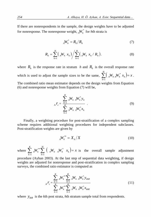
254 A. Alkaya, H. Ö. Ayhan, A. Esin: Sequential data…
If there are nonrespondents in the sample, the design weights have to be adjusted
for nonresponse. The nonresponse weight,*
hAW for hth strata is
hhA RRW 0
* (7)
H
h
hhhA
H
h
hhA RxWxWR11
0 / . (8)
where hR is the response rate in stratum h and 0R is the overall response rate
which is used to adjust the sample sizes to be the same, xxWWH
h
hhAhA 1
*.
The combined ratio mean estimator depends on the design weights from Equation
(6) and nonresponse weights from Equation (7) will be,
cAr =
H
h
hhAhA
H
h
hhAhA
xWW
yWW
1
*
1
*
. (9)
Finally, a weighting procedure for post-stratification of a complex sampling
scheme requires additional weighting procedures for independent subclasses.
Post-stratification weights are given by
**
kAW XX k (10)
where xxWWWK
k
H
h
khAhAkA 1 1
***is the overall sample adjustment
procedure (Ayhan 2003). At the last step of sequential data weighting, if design
weights are adjusted for nonresponse and post-stratification in complex sampling
surveys, the combined ratio estimator is computed as
cAr =
H
h
khRhAhA
K
k
kA
H
h
khRhAhA
K
k
kA
xWWW
yWWW
1
*
1
**
1
*
1
**
(11)
where khRy is the kth post strata, hth stratum sample total from respondents.

STATISTICS IN TRANSITION new series, June 2017
255
4. General variance estimation for the population ratio estimator
Although weighting data or sequential data weighting procedures are
commonly used, it can be difficult to estimate sampling variances of associated
weighted estimates. Lu and Gelman (2003) proposed a method for estimating the
sampling variances of survey estimates with weighting adjustments derived from
design-based analytic and Taylor-series variance estimators of population mean
estimator in a general way. A natural simplifying assumption is to pretend that the
weighting is all inverse-probability, with independent sampling where the
probability that unit i is selected with proportional to ii W/1 . To compute the
variance for inverse-probability weighting, a general variance estimator for
Y acknowledged as a ratio form of the weighted mean
n
i i
n
i ii
W
yW
1
1 (12)
where the denominator of this expression is 1, but only after the weights have
normalized. The variance of is given by
n
i
iiHT yWV1
22 )ˆ()ˆ(ˆ (13)
and n
iW =1 (Lu and Gelman 2003).
Taylor-series method consists of deriving from a complex non-linear statistic,
a linear statistic which has the same asymptotic variance
n
i
ii zWVV1
ˆ)ˆ(ˆ (14)
where iz new variable whose expression depends on and called a linearized
variable for . When xy /ˆ then iii xyz , ni ,...,1 (Osier and
Museux 2006). Mean of this variable is 0 XRYZ . Therefore, in a
weighted sample the variance estimation of mean z is
n
i
iii xxryyWN
zV1
22
2)()(
1)(ˆ (15)
General variance estimation for the estimators of population ratio R , the
linear relation can be expressed by bxy . In weighted data for the variance
estimation of population ratio estimator is given by Taylor-series method as using
variable iii xyz , where xyr /ˆ , the variable sample mean is

256 A. Alkaya, H. Ö. Ayhan, A. Esin: Sequential data…
xyz and population total estimate is zN . Thereby, since r then the
variance estimation of r is
n
i
iii xxryyWX
rV1
22
2)()(
1)(ˆ
(16)
A general equation for variance estimation of the population ratio estimator
under stratified random sampling design depending on Taylor-series method can
be introduced depending on Equation (16). A new variable defined as
hihihi xyz , where cr . Since this variable sample mean is
ststst xyz and population total estimate is stzN . Here
H
h hhst yNNy1
1 and
H
h hhst xNNx1
1 are the standard estimates of
the population means Y and X , respectively, made from a stratified sample.
Mean of the new variable is 0 XRYZ . Thereby, under stratified random
sampling design the variance estimation of stz ,
H
h
zhhst sWN
zV1
22
2
1)(ˆ ,
h
h
hn
NW (17)
H
h
n
i
hhichhihst
h
xxryyWN
zV1 1
22
2)()(
1)(ˆ (18)
Where hn is the sample size of stratum h, hiy is the ith value of variable y in
stratum h, hix is the ith value of variable x in stratum h (here )1( hf are
neglected where hf is the sampling fraction for hth stratum). Therefore, defining
iii xyz and cr , the variance estimation can be obtained as
)(ˆ strV
H
h
n
i
hhichhih
h
xxryyWX 1 1
22
2)()(
1 (19)
This general variance estimation formulation for the stratified sampling
design can also be extended to be the basis for the other complex sampling
designs.
5. Variance inflation factor in the comparison of the weighting
methods
The variability of weights increases, thereby the accuracy of estimates
decreases. A useful measure of the accuracy of this loss is the variance inflation
factor (VIF). VIF which is adopted to be the variability measure of weights can
be used for comparing the weights and weighting methods. The measure VIF
STATISTICS IN TRANSITION new series, June 2017
257
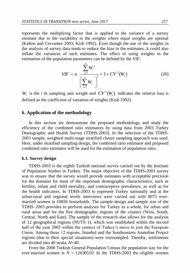
represents the multiplying factor that is applied to the variance of a survey
estimate due to the variability in the weights where equal weights are optimal
(Kalton and Cervantes 2003; Kish 1992). Even though the use of the weights in
the analysis of survey data tends to reduce the bias in the estimates, it could also
inflate the variances of such estimates. The effect of using weights in the
estimation of the population parameters can be defined by the VIF,
2
1
1
2
n
i
i
n
i
i
W
W
nVIF = )(1 2
iWCV (20)
iW is the i th sampling unit weight and )(2
iWCV indicates the relative loss is
defined as the coefficient of variation of weights (Kish 1992).
6. Application of the methodology
In this section we demonstrate the proposed methodology and study the
efficiency of the combined ratio estimators by using data from 2003 Turkey
Demographic and Health Survey (TDHS-2003). In the selection of the TDHS-
2003 sample, weighted multi-stage stratified cluster sampling approach was used.
Here, under stratified sampling design, the combined ratio estimator and proposed
combined ratio estimator will be used for the estimation of population ratio.
6.1. Survey design
TDHS-2003 is the eighth Turkish national survey carried out by the Institute
of Population Studies in Turkey. The major objective of the TDHS-2003 survey
was to ensure that the survey would provide estimates with acceptable precision
for the domains for most of the important demographic characteristics, such as
fertility, infant and child mortality, and contraceptive prevalence, as well as for
the health indicators. In TDHS-2003 to represent Turkey nationally and at the
urban-rural and regional levels interviews were carried out with 8075 ever-
married women in 10836 households. The sample design and sample size of the
TDHS–2003 provides to perform analyses for Turkey as a whole, for urban and
rural areas and for the five demographic regions of the country (West, South,
Central, North and East). The sample of the research also allows for the analysis
of 12 geographical regions (NUTS 1), which was established within the second
half of the year 2002 within the context of Turkey’s move to join the European
Union. Among these 12 regions, İstanbul and the Southeastern Anatolian Project
regions (due to their special situations) were oversampled. Thereby, settlements
are divided into 40 strata, H=40.
From the 2000 Turkish General Population Census the population size for the
ever-married women is N = 12630510. In the TDHS-2003 the eligible women
258 A. Alkaya, H. Ö. Ayhan, A. Esin: Sequential data…
were identified as 8477 of whom 96 percent were interviewed and so interviews
were carried out with 8075 ever-married women.
6.2. Two variable ratio estimation
One of the objectives of this paper is to measure a population ratio. Using data
from the TDHS-2003, we have decided to examine the ratio of the number of live
births to the number of living children of ever-married women. Therefore, y ,
indicates the number of living children and x , indicates the number of live births.
R XY / Number of living children / Number of live births will be estimated.
In the estimation of R the known combined ratio estimator c
r and Ayhan
(2003)’s proposed combined ratio estimator cA
r are used and the comparison of
the c
r and
cAr estimates are illustrated in the following sections.
The initial information on all places of residences in Turkey was derived from
the year 2000 Turkish General Population Census results which provided a
computerized list of all settlements (provincial and district, sub-districts and
villages), their populations and the households. From 2000 Turkish General
Population Census results, the true population ratio for the ever-married women is
XYR / 30398682/32713021 = 0.929253 and this means in Turkey nearly
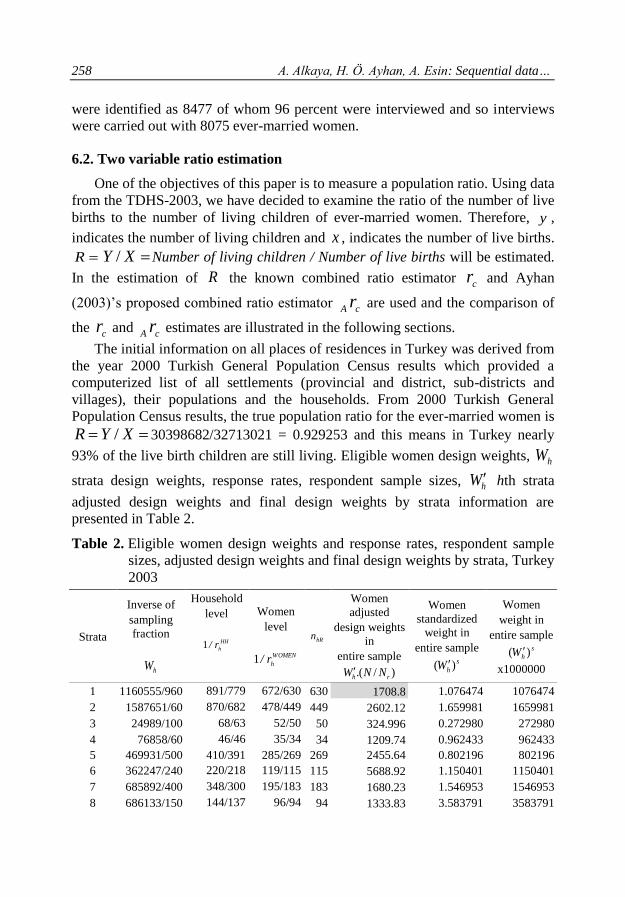
93% of the live birth children are still living. Eligible women design weights, hW
strata design weights, response rates, respondent sample sizes, hW hth strata
adjusted design weights and final design weights by strata information are
presented in Table 2.
Table 2. Eligible women design weights and response rates, respondent sample
sizes, adjusted design weights and final design weights by strata, Turkey
2003
Strata
Inverse of
sampling
fraction
hW
Household
level
HH
hr/1
Women
level
WOMEN
hr/1
Women
adjusted
design weights
in
entire sample
)/.( rh NNW
Women
standardized
weight in
entire sample s
hW )(
Women
weight in
entire sample s
hW )(
x1000000
1 1160555/960 891/779 672/630 630 1708.8 1.076474 1076474
2 1587651/60 870/682 478/449 449 2602.12 1.659981 1659981
3 24989/100 68/63 52/50 50 324.996 0.272980 272980
4 76858/60 46/46 35/34 34 1209.74 0.962433 962433
5 469931/500 410/391 285/269 269 2455.64 0.802196 802196
6 362247/240 220/218 119/115 115 5688.92 1.150401 1150401
7 685892/400 348/300 195/183 183 1680.23 1.546953 1546953
8 686133/150 144/137 96/94 94 1333.83 3.583791 3583791
hRn

STATISTICS IN TRANSITION new series, June 2017
259
Table 2. Eligible women design weights and response rates, respondent sample
sizes, adjusted design weights and final design weights by strata, Turkey
2003 (cont.)
Strata
Inverse of
sampling
fraction
hW
Household
level
HH
hr/1
Women
level
WOMEN
hr/1
Women
adjusted
design
weights in
entire sample
)/.( rh NNW
Women
standardized
weight in
entire sample s
hW )(
Women
weight in
entire sample s
hW )(
x1000000
9 667273/240 211/204 139/135 135 1655.51 2.305124 2305124
10 202772/150 129/127 94/89 89 5173.43 1.058475 1058475
11 211704/60 48/47 50/48 48 2235.38 2.739621 2739621
12 352876/400 348/300 225/200 200 598.79 0.840259 840259
13 129118/100 83/75 46/46 46 2734.71 1.042909 1042909
14 109307/60 33/33 27/26 26 3442.6 1.841054 1841054
15 377921/100 90/86 70/62 62 846.61 3.259059 3259059
16 148605/60 56/56 39/38 38 1587.51 1.855263 1855263
17 182284/100 86/85 68/65 65 1305.67 1.408203 1408203
18 65446/60 45/45 21/21 21 867.53 0.796109 796109
19 47999/100 80/77 57/55 55 1349.47 0.377212 377212
20 83237/60 55/55 44/43 43 641.78 1.036076 1036076
21 915073/500 451/386 287/260 260 513.44 1.722755 1722755
22 431779/150 128/124 99/99 99 945.73 2.168697 2168697
23 298404/240 173/172 116/107 107 946.82 1.130884 1130884
24 276431/400 361/349 276/270 270 1527.76 0.533328 533328
25 1052242/900 808/734 593/557 557 1826.15 1.028638 1028638
26 681896/540 470/446 302/286 286 3430.47 1.085906 1085906
27 523267/500 457/438 354/343 343 4348.88 0.822517 822517
28 373756/240 210/205 162/159 159 2191.87 1.186317 1186317
29 336258/500 427/395 275/267 267 2945.04 0.546506 546506
30 318422/240 207/204 156/153 153 1263.75 1.001856 1001856
31 224473/200 180/176 138/136 136 1644.66 0.850111 850111
32 201222/90 82/82 60/59 59 1570.77 1.659488 1659488
33 310851/600 497/474 362/355 355 1628.01 0.404297 404297
34 349165/240 203/199 136/126 126 1883.16 1.169152 1169152
35 212359/500 462/452 392/384 384 1590.35 0.323444 323444
36 218260/240 200/199 158/151 151 2634.27 0.797725 797725
37 371366/500 478/449 383/371 371 1855.92 0.595771 595771
38 257644/240 227/220 208/195 195 1108.02 0.862345 862345
39 756933/1000 922/877 762/742 742 1368.89 0.596458 596458
40 356146 / 480 455 / 449 416 / 403 403 899.22 0.566475 566475
Source: TDHS 2003
hRn
260 A. Alkaya, H. Ö. Ayhan, A. Esin: Sequential data…
The nonresponse adjustments for the sampling weights hW are conducted at
each strata, Hh ,...,1 .
The adjusted nonresponse weights hW (HH
hr/1 ) (WOMEN
hr/1 ) are defined by
multiplying sampling weights by the inverse of household and women level
response ratios. However, to provide equality of the adjusted sampling weights
total to the population total, the adjusted sampling weights hW (HH
hr/1 )(
WOMEN
hr/1 ) are multiplied with the value of,
H
h
WOMEN
h
HH
h
nhR
i h rrWN1 1
)/1)(/1( = 12630510/10901679 = 1.158584.
Thus, the adjusted sampling weights are presented as )/.( rh NNW in Table 2.
For example, the calculation for the adjusted value hW = 1474.9 from Table 3 is
as,
)/.( hh NNW = (1160555/960) (891/ 779) (672 / 630) 1.158584 = 1474.9(1.158584)
= 1708.799. Hence, hW used for design weights hW .
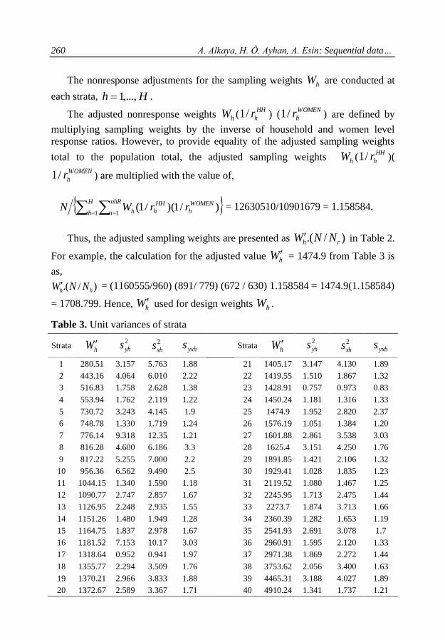
Table 3. Unit variances of strata
Strata hW
2
yhs 2
xhs yxhs
Strata hW
2
yhs 2
xhs yxhs
1 280.51 3.157 5.763 1.88 21 1405.17 3.147 4.130 1.89
2 443.16 4.064 6.010 2.22 22 1419.55 1.510 1.867 1.32
3 516.83 1.758 2.628 1.38 23 1428.91 0.757 0.973 0.83
4 553.94 1.762 2.119 1.22 24 1450.24 1.181 1.316 1.33
5 730.72 3.243 4.145 1.9 25 1474.9 1.952 2.820 2.37
6 748.78 1.330 1.719 1.24 26 1576.19 1.051 1.384 1.20
7 776.14 9.318 12.35 1.21 27 1601.88 2.861 3.538 3.03
8 816.28 4.600 6.186 3.3 28 1625.4 3.151 4.250 1.76
9 817.22 5.255 7.000 2.2 29 1891.85 1.421 2.106 1.32
10 956.36 6.562 9.490 2.5 30 1929.41 1.028 1.835 1.23
11 1044.15 1.340 1.590 1.18 31 2119.52 1.080 1.467 1.25
12 1090.77 2.747 2.857 1.67 32 2245.95 1.713 2.475 1.44
13 1126.95 2.248 2.935 1.55 33 2273.7 1.874 3.713 1.66
14 1151.26 1.480 1.949 1.28 34 2360.39 1.282 1.653 1.19
15 1164.75 1.837 2.978 1.67 35 2541.93 2.691 3.078 1.7
16 1181.52 7.153 10.17 3.03 36 2960.91 1.595 2.120 1.33
17 1318.64 0.952 0.941 1.97 37 2971.38 1.869 2.272 1.44
18 1355.77 2.294 3.509 1.76 38 3753.62 2.056 3.400 1.63
19 1370.21 2.966 3.833 1.88 39 4465.31 3.188 4.027 1.89
20 1372.67 2.589 3.367 1.71 40 4910.24 1.341 1.737 1.21

STATISTICS IN TRANSITION new series, June 2017
261
6.3. Combined ratio estimator
Combined ratio estimator for R is
cr =
H
h
hh
H
h
hh
xW
yW
1
1 =33214885
30466444 = 0.917253.
This means that, the ever-married women, 91.7% of live born children are
estimated to have lived. A general variance estimation proposed for the
population ratio which is given by Equation (19) can be written as,
H
h
xhcyxhcyh
h
hc srsrsn
WX
rV1
2222
22
11)(ˆ . (21)
The variance estimation of combined ratio estimator (conventional combined
ratio estimator) depending on hW adjusted weights is
H
h
xhcyxhcyh
h
hcsrsrs
nW
X)r(V
1
2222
22
11
)r(Vc
(3.22) 10 –9.
2
yhs , yxhs , 2
xhs computed unit variance values of the strata are given in Table 3.
There is an increase in the variance of the ratio estimate due to the use of design
weights hW , and so that the VIF value is obtained as:
VIF (hW ) =
2
1
'
1
2' )(H
h
h
H
h
h WWH = 1.387289
For a VIF≈1.387, i.e., a reduction in the effective sample size of almost 38.7
percent.
6.4. Proposed combined ratio estimator
The estimator was proposed under sequential weighting process and so on the
design weights are adjusted for nonresponse and post-stratification in TDHS-
2003. First step is to obtain design weights hAW . Second step is to compute
nonresponse weights *
hAW . The final step is weighting for post-stratification that
is conducted by **
kAW . Here, h=1,..,H, H=40. The hAW weight results are
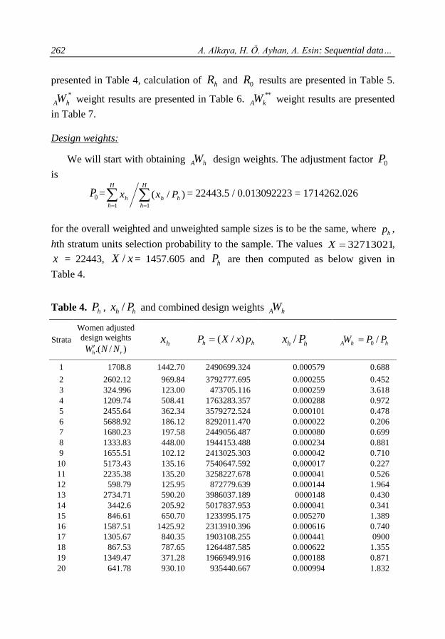
262 A. Alkaya, H. Ö. Ayhan, A. Esin: Sequential data…
presented in Table 4, calculation of hR and 0R results are presented in Table 5.
*
hAW weight results are presented in Table 6. **
kAW weight results are presented
in Table 7.
Design weights:
We will start with obtaining hAW design weights. The adjustment factor 0P
is
0P =
H
h
hh
H
h
h Pxx11
)/( = 22443.5 / 0.013092223 = 1714262.026
for the overall weighted and unweighted sample sizes is to be the same, where hp ,
hth stratum units selection probability to the sample. The values 32713021X ,
x = 22443, xX / = 1457.605 and hP are then computed as below given in
Table 4.
Table 4. hP , hh Px / and combined design weights hAW
Strata
Women adjusted
design weights
)/.( rh NNW hx hh pxXP )/(
hh Px / hhA PPW /0
1 1708.8 1442.70 2490699.324 0.000579 0.688
2 2602.12 969.84 3792777.695 0.000255 0.452
3 324.996 123.00 473705.116 0.000259 3.618
4 1209.74 508.41 1763283.357 0.000288 0.972
5 2455.64 362.34 3579272.524 0.000101 0.478
6 5688.92 186.12 8292011.470 0.000022 0.206
7 1680.23 197.58 2449056.487 0.000080 0.699
8 1333.83 448.00 1944153.488 0.000234 0.881
9 1655.51 102.12 2413025.303 0.000042 0.710
10 5173.43 135.16 7540647.592 0,000017 0.227
11 2235.38 135.20 3258227.678 0.000041 0.526
12 598.79 125.95 872779.639 0.000144 1.964
13 2734.71 590.20 3986037.189 0000148 0.430
14 3442.6 205.92 5017837.953 0.000041 0.341
15 846.61 650.70 1233995.175 0.005270 1.389
16 1587.51 1425.92 2313910.396 0.000616 0.740
17 1305.67 840.35 1903108.255 0.000441 0900
18 867.53 787.65 1264487.585 0.000622 1.355
19 1349.47 371.28 1966949.916 0.000188 0.871
20 641.78 930.10 935440.667 0.000994 1.832

STATISTICS IN TRANSITION new series, June 2017
263
Table 4. hP , hh Px / and combined design weights hAW (cont.)
Strata
Women adjusted
design weights
)/.( rh NNW hx hh pxXP )/(
hh Px / hhA PPW /0
21 513.44 1025.28 748375.855 0.001370 2.290
22 945.73 953.47 1378469.728 0.000691 1.243
23 946.82 2144.38 1380058.482 0.001553 1,242
24 1527.76 78.88 2226820.459 0.000035 0.769
25 1826.15 354.20 2661745.418 0.000133 0.644
26 3430.47 449.55 5000157.602 0.000089 0.342
27 4348.88 171.84 6338806.459 0.000027 0.270
28 2191.87 85.02 3194808.713 0.000026 0.536
29 2945.04 152.00 4292608.344 0.000035 0.399
30 1263.75 68.04 1842006.830 0.000036 0.930
31 1644.66 107.07 2397210.645 0.000044 0.715
32 1570.77 254.66 2289510.638 0.000112 0.748
33 1628.01 1092.52 2372942,069 0.000460 0.722
34 1883.16 605.79 2744841.608 0.000220 0.624
35 1590.35 602.82 2318049.901 0.000260 0.739
36 2634.27 207.09 3839638.641 0.000053 0.446
37 1855.92 375.48 2705137.342 0.000138 0.633
38 1108.02 418.27 1615019.116 0.000258 1.061
39 1368.89 783.90 1995255.968 0.000392 0.859
40 899.22 1974.70 1310678.047 0.001506 1.307
Total 22443.50 0.013092
Nonresponse weights:
In TDHS–2003, there are also non-respondent women in the survey.
A weighting procedure for nonresponse is essential so we should adjust the design
weights by assigning nonresponse weights to the data. Table 5 presents the
calculation of the response rates hR .
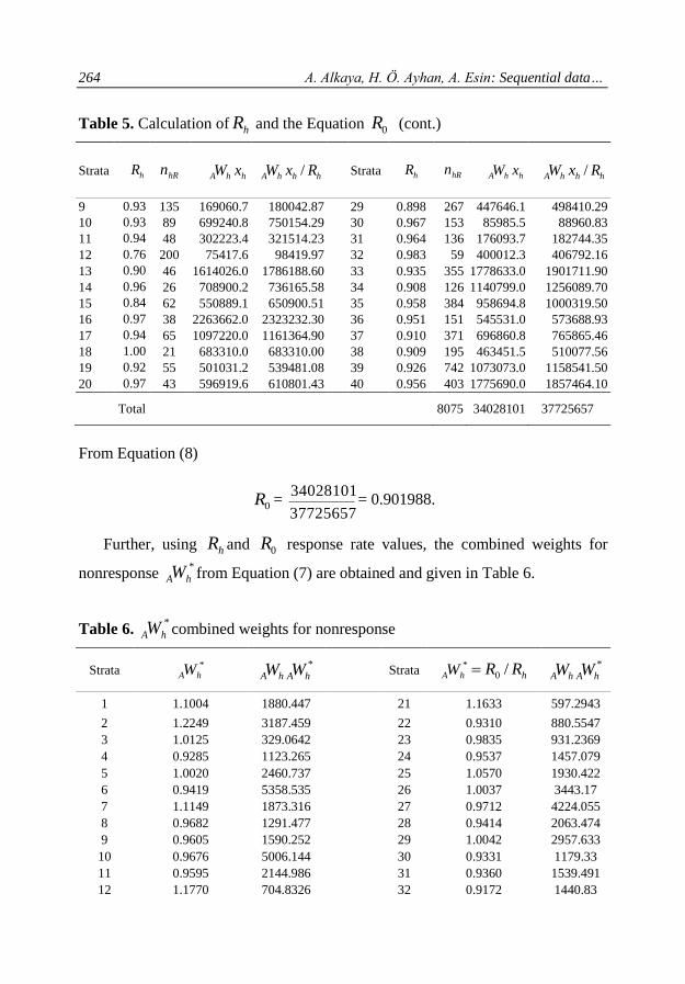
Table 5. Calculation of hR and the Equation 0R
Strata hR hhA xW
hhhA RxW / Strata hR hhA xW
hhhA RxW /
1 0.82
0 630 2465286.0 3007711.90 21 0.775 260 526419.8 678937.77
2 0.73
6 449 2523640.0 3427234.70 22 0.969 99 901725.2 930813.09
3 0.89
1 50 39974.5 44872.97 23 0.917 107 2030342.0 2213915.50
4 0.97
1 34 615043.9 633133.44 24 0.946 270 120509.7 127423.38
5 0.90
0 269 889776.6 988509.07 25 0.853 557 646822.3 758053.41
6 0.95
8 115 1058822.0 1105702.20 26 0.899 286 1542168.0 1716072.10
7 0.80
9 183 331979.8 410348.86 27 0.929 343 747311.5 804735.05
8 0.93
2 94 597555.8 641451.46 28 0.958 159 186352.8 194499.83
hRn hRn
264 A. Alkaya, H. Ö. Ayhan, A. Esin: Sequential data…
Table 5. Calculation of hR and the Equation 0R (cont.)
Strata hR hhA xW
hhhA RxW / Strata hR hhA xW
hhhA RxW /
9 0.93
9 135 169060.7 180042.87 29 0.898 267 447646.1 498410.29
10 0.93
2 89 699240.8 750154.29 30 0.967 153 85985.5 88960.83
11 0.94
0 48 302223.4 321514.23 31 0.964 136 176093.7 182744.35
12 0.76
6 200 75417.6 98419.97 32 0.983 59 400012.3 406792.16
13 0.90
4 46 1614026.0 1786188.60 33 0.935 355 1778633.0 1901711.90
14 0.96
3 26 708900.2 736165.58 34 0.908 126 1140799.0 1256089.70
15 0.84
6 62 550889.1 650900.51 35 0.958 384 958694.8 1000319.50
16 0.97
4 38 2263662.0 2323232.30 36 0.951 151 545531.0 573688.93
17 0.94
5 65 1097220.0 1161364.90 37 0.910 371 696860.8 765865.46
18 1.00
0 21 683310.0 683310.00 38 0.909 195 463451.5 510077.56
19 0.92
9 55 501031.2 539481.08 39 0.926 742 1073073.0 1158541.50
20 0.97
7 43 596919.6 610801.43 40 0.956 403 1775690.0 1857464.10
Total 8075 34028101 37725657
From Equation (8)
0R = 37725657
34028101= 0.901988.
Further, using hR and 0R response rate values, the combined weights for
nonresponse *
hAW from Equation (7) are obtained and given in Table 6.
Table 6. *
hAW combined weights for nonresponse
Strata *
hAW *
hAhA WW Strata *
hAW hRR /0 *
hAhA WW
1 1.1004 1880.447
21 1.1633 597.2943
2 1.2249 3187.459 22 0.9310 880.5547
3 1.0125 329.0642 23 0.9835 931.2369
4 0.9285 1123.265 24 0.9537 1457.079
5 1.0020 2460.737 25 1.0570 1930.422
6 0.9419 5358.535 26 1.0037 3443.17
7 1.1149 1873.316 27 0.9712 4224.055
8 0.9682 1291.477 28 0.9414 2063.474
9 0.9605 1590.252 29 1.0042 2957.633
10 0.9676 5006.144 30 0.9331 1179.33
11 0.9595 2144.986 31 0.9360 1539.491
12 1.1770 704.8326 32 0.9172 1440.83
hRn hRn
STATISTICS IN TRANSITION new series, June 2017
265
Table 6. *
hAW combined weights for nonresponse (cont.)
Strata *
hAW *
hAhA WW Strata *
hAW hRR /0 *
hAhA WW
13 0.9982 2729.789
33 0.9644 1570.06
14 0.9366 3224.615 34 0.9931 1870.249
15 1.0657 902.2662 35 0.9411 1496.759
16 0.9257 1469.597 36 0.9485 2498.724
17 0.9547 1246.549 37 0.9913 1839.783
18 0.9019 782.5019 38 0.9927 1099.969
19 0.9712 1310.616 39 0.9738 1333.067
20 0.9229 592.3403 40 0.9435 848.4382
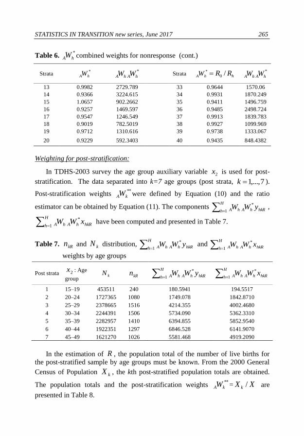
Weighting for post-stratification:
In TDHS-2003 survey the age group auxiliary variable 2x is used for post-
stratification. The data separated into k=7 age groups (post strata, 7,...,1k ).
Post-stratification weights **
kAW were defined by Equation (10) and the ratio
estimator can be obtained by Equation (11). The components
H
h hkRhAhA yWW1
* ,
H
h hkRhAhA xWW1
* have been computed and presented in Table 7.
Table 7. kRn and kN distribution,
H
h hkRhAhA yWW1
*
and
H
h hkRhAhA xWW1
*
weights by age groups
Post strata 2x : Age
group kN
kRn
H
h hkRhAhA yWW1
*
H
h hkRhAhA xWW1
*
1 15–19 453511 240 180.5941 194.5517
2 20–24 1727365 1080 1749.078 1842.8710
3 25–29 2378665 1516 4214.355 4002.4680
4 30–34 2244391 1506 5734.090 5362.3310
5 35–39 2282957 1410 6394.855 5852.9540
6 40–44 1922351 1297 6846.528 6141.9070
7 45–49 1621270 1026 5581.468 4919.2090
In the estimation of R , the population total of the number of live births for
the post-stratified sample by age groups must be known. From the 2000 General
Census of Population kX , the kth post-stratified population totals are obtained.
The population totals and the post-stratification weights **
kAW = XX k / are
presented in Table 8.
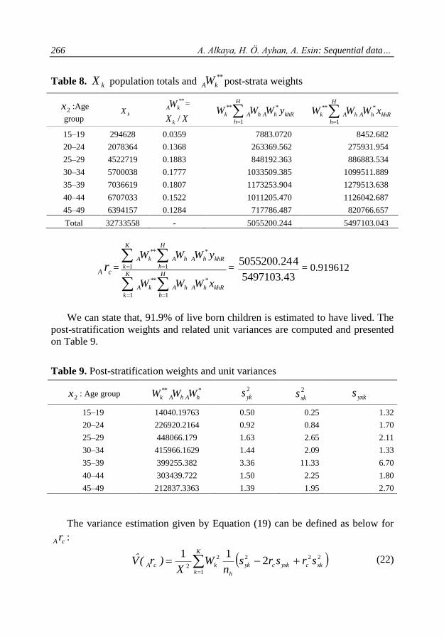
266 A. Alkaya, H. Ö. Ayhan, A. Esin: Sequential data…
Table 8. kX population totals and
**
kAW post-strata weights
2x :Age
group kX
**
kAW =
XX k /
H
h
khRhAhAk yWWW1
***
H
h
khRhAhAk xWWW1
***
15–19 294628 0.0359 7883.0720 8452.682
20–24 2078364 0.1368 263369.562 275931.954
25–29 4522719 0.1883 848192.363 886883.534
30–34 5700038 0.1777 1033509.385 1099511.889
35–39 7036619 0.1807 1173253.904 1279513.638
40–44 6707033 0.1522 1011205.470 1126042.687
45–49 6394157 0.1284 717786.487 820766.657
Total 32733558 - 5055200.244 5497103.043
cAr =
H
h
khRhAhA
K
k
kA
H
h
khRhAhA
K
k
kA
xWWW
yWWW
1
*
1
**
1
*
1
**
= 5497103.43
45055200.24= 0.919612
We can state that, 91.9% of live born children is estimated to have lived. The
post-stratification weights and related unit variances are computed and presented
on Table 9.
Table 9. Post-stratification weights and unit variances
2x : Age group ***
hAhAk WWW 2
yks 2
xks yxks
15–19 14040.19763 0.50 0.25 1.32
20–24 226920.2164 0.92 0.84 1.70
25–29 448066.179 1.63 2.65 2.11
30–34 415966.1629 1.44 2.09 1.33
35–39 399255.382 3.36 11.33 6.70
40–44 303439.722 1.50 2.25 1.80
45–49 212837.3363 1.39 1.95 2.70
The variance estimation given by Equation (19) can be defined as below for
cAr :
K
k
xkcyxkcyk
h
kcAsrsrs
nW
X)r(V
1
2222
22
11
(22)

STATISTICS IN TRANSITION new series, June 2017
267
The variance estimation value is
)(ˆ cArV (2.9) 10 –9
where ***
hAhAkk WWWW and
2
yks 2
xks unit variances of k th poststrata for y and
x, respectively and yxks is covariance of k th poststrata for y and x. Inflation
factor for kW obtained as 1.238408)( kWVIF . There is nearly 10% reduction in
the VIF value of proposed ratio estimator relative to conventional combined ratio
estimator. VIF is reduced from 1.387 with conventional combined ratio estimator
to 1.238 with proposed ratio estimator.
The comparison of the conventional combined ratio estimator and the
proposed combined ratio estimator results of means, variance estimations and
VIF are given on Table 10. In Table 10, we observe the values of mean, variance
estimation and VIF of the combined ratio estimator and the proposed combined
ratio estimator. From Table 10, it can be concluded that the proposed combined
ratio estimator has the minimum variance estimation but it is seen that both have
approximate variance estimation values. The variability level of weights
according VIF values cA
r seems as less variable thanc
r .
Table 10. The comparisons of combined ratio estimator results
Mean )ˆ(ˆ HTV VIF
Conventional combined
ratio estimator cr = 0.917 (3.2) 10 –9 VIF (
hW ) = 1.387289
Ayhan (2003)’s combined
ratio estimator cAr = 0.919 (2.9) 10 –9 VIF ( ***
hAhAk WWW ) = 1.238408
7. Conclusions
Researchers believe that, the weights that provide excellent estimates for
auxiliary variables will also provide good estimates for the interest variable. The
new weights will continue to give unbiased estimates, but a realistic expectation is
to remain near unbiasedness (Deville and Särndal 1992). Using the data weighted
according to the auxiliary variable(s) which are known to be related to the interest
variable lead to additional gains in the information. The weights in the combined
ratio estimator cAr are defined on the basis of population and sample sizes and
also information on the auxiliary variable. TDHS-2003 results have shown that,
the combined ratio estimator which is defined by Ayhan (2003) provided a better

268 A. Alkaya, H. Ö. Ayhan, A. Esin: Sequential data…
estimate of the parameter, by using auxiliary variable values in the calculation of
weights. The proposed estimator has lower variance; it is not enough to prove that
it is more efficient. The variance could be underestimated. We can say that, the
estimator better reflects the effect of post-stratification.
REFERENCES
ARDILLY, P., TILLE, Y., (2006). Sampling methods: exercises and solutions.
Translated from French by Leon Jang. Springer Science+Business Media, USA.
AYHAN, H. Ö., (1981). Sources and bias of nonresponse in the Turkish Fertility Survey
1978, Turkish Journal of Population Studies 2–3, pp. 104–148.
AYHAN, H. Ö., (1991). Post–stratification and weighting in sample surveys. Invited
paper, Research Symposium '91, State Institute of Statistics, Ankara.
AYHAN, H. Ö., (2003). Combined weighting procedures for post-survey adjustment in
complex sample surveys. Bulletin of the International Statistical Institute, 60 (1),
pp. 53–54.
BETHLEHEM, J. G., KERSTEN, H. M. P., (1985). On the treatment of nonresponse in
sample surveys. Journal of Official Statistics, 1 (3), pp. 287–300.
BETHLEHEM, J. G., KELLER, W. J., (1987). Linear weighting of the sample survey
data. Journal of Official Statistics, 3 (2), pp. 141–153.
CASSEL, C. M., SÄRNDAL, C. E., WRETMAN J. H., (1976). Some results on
generalized difference estimation and generalized regression estimation for finite
populations. Biometrika, 63, pp. 615–620.
CERVANTES, I. F., BRICK, J. F., (2009). Efficacy of Poststratification in Complex
Sample Design. Proceedings of the Survey Research Methods Section, American
Statistical Association, pp. 4642–4655.
COCHRAN, W. G., (1977). Sampling Techniques. 3rd ed. Wiley, New York.
DEMING, W. E., STEPHAN, F. F., (1940). On a least squares adjustment of a sample
frequency table when the expected marginal totals are known. Annals of
Mathematical Statistics, 11 (4), pp. 427–444.
DEVILLE, J. C., SARNDAL, C. E., (1992). Calibration estimators in survey sampling.
Journal of the American Statistical Association, 87, pp. 376–382.
DEVILLE, J. C., SARNDAL, C. E., SAUTORY, O., (1993). Generalized raking
procedure in survey sampling. Journal of the American Statistical Association, 88,
pp. 1013–1020.
ESTEVAO, V. M., SÄRNDAL, C. E., (2000). A functional form approach to calibration.
Journal of Official Statistics, 16 (4), pp. 379–399.
GUY, P. W., (1979). Small sample theory for poststratification, Doctor of Philosophy,
Graduate College of Texas ASM University, Texas.

STATISTICS IN TRANSITION new series, June 2017
269
HAJEK, J., (1971). Comment on a paper of D. Basu, In Foundations of Statistical
Inference, Toronto, pp. 236–237.
HOLT, D., ELLIOT, D., (1991). Methods of weighting for unit non-response. The
Statistician, 40, pp. 333–342.
HOLT, D., SMITH, T. M. F., (1979). Post stratification. Journal of the Royal Statistical
Society, Series A (General), 142 (1), pp. 33–46.
HORVITZ, D. G., THOMPSON, D. J., (1952). A generalization of sampling without
replacement from a finite universe. Journal of the American Statistical Association,
47, pp. 663–685.
ISAKI, C. T., FULLER, W. A., (1982). Survey design under the regression
superpopulation model. Journal of the American Statistical Association, 77,
pp. 89–96.
KALTON, G., CERVANTES, F. I., (2003). Weighting methods. Journal of Official
Statistics, 19 (2), pp. 81–97.
KISH, L., (1965). Survey Sampling. John Wiley & Sons, Inc., USA.
KISH, L., (1992). Weighting for unequal Pi. Journal of Official Statistics, 8 (2), pp. 183–
200.
KOTT, P. S., (2006). Using calibration weighting to adjust for nonresponse and coverage
errors. Survey Methodology, 32, pp. 133–142.
LITTLE, R. J. A., (1993). Post-stratification: A modeler’s perspective, Journal of The
American Statistical Association, 88, pp. 1001–1012.
LITTLE, R. J. A., VARTIVARIAN, S., (2005). Does weighting for nonresponse increase
the variance of survey means? Proceedings of American Statistical Association:
Section on Survey Research Methods, Minneapolis, pp. 3897–3904.
LU H., GELMAN, A., (2003). A method for estimating design based sampling variances
for surveys with weighting, post-stratification, and raking. Journal of Official
Statistics, 19(2), pp. 133–151.
OSIER, G., MUSEUX, J. M., (2006). Variance estimation for EU–SILC complex poverty
indicators using linearization techniques. European Conference on Quality in
Survey Statistics, Luxembourg, pp. 1–11.
SÄRNDAL, C. E., (1980). On -inverse weighting versus best linear unbiased weighting
in probability sampling, Biometrika, 67, pp. 639–650.
SÄRNDAL, C. E., SWENSON, B., WRETMAN, J., (1992). Model assisted survey
sampling. Springer–Verlag, New York.
SÄRNDAL, C. E., (2007). The calibration approach in survey theory and practice. Survey
Methodology, Statistics Canada, 33 (2), pp. 99–119.
SINGH, S., (2003). Advanced sampling theory with applications. Kluwer Academic
Publishers, Dordrecht Boston, London.
SMITH, T. M. F., (1991). Post–stratification. The Statistician, 40, pp. 315–321.

270 A. Alkaya, H. Ö. Ayhan, A. Esin: Sequential data…
STEPHAN, F. F., (1942). An iterative method of adjusting sample frequency tables when
expected marginal totals are known. Annals of Mathematical Statistics, 13 (2),
pp. 166–178.
TDHS, (2004). Turkey Demographic and Health Survey 2003. Hacettepe University,
Institute of Population Studies, Ankara, Turkey.
TIKKIWAL, G. C., RAI, P. K., GHIYA, A., (2013). On the Performance of Generalized
Regression Estimator for Small Domains, Communication in Statistics: Simulation
and Computation, 42, pp. 891–909.
VERMA, V., (1991). Sampling Methods. Manual for Statistical Trainers Number 2,
Statistical Institute for Asia and the Pacific, Tokyo, Japan.
VERMA, V., (2007). Recent advances in survey sampling. In: Ayhan, H.Ö. and Batmaz,
I. (eds.), Recent Advances in Statistics. Turkish Statistical Institute Press, Ankara,
Turkey, pp. 77–101.
WRIGHT, R. L., (1983). Finite population sampling with multivariate auxiliary
information. Journal of the American Statistical Association, 78, pp. 879–884.
WU, C., SITTER, R. R., (2001). A model-calibration approach to using complete
auxiliary information from survey data. Journal of the American Statistical
Association, 96, pp. 185–193.
WU, C., (2003). Optimal calibration estimators in survey sampling. Biometrika, 90(4),
pp. 937–951.