Sequential data analysis An introduction to R -...

Sequential data analysis

Sequential data analysisAn introduction to R

Gilbert Ritschard

Department of Econometrics and Laboratory of Demography, University ofGeneva

http://mephisto.unige.ch/biomining

APA-ATI Workshop on Exploratory Data MiningUniversity of Southern California, Los Angeles, CA, July 2009

23/7/2009gr 1/64

http://mephisto.unige.ch/biomining


Outline

1 Introduction

2 Installing and launching R

3 Objects and operators

4 Elements of statistical modeling

5 Growing trees: rpart and party

6 Custom functions and programming

23/7/2009gr 2/64


Introduction

Outline

1 Introduction






23/7/2009gr 3/64


Introduction

R

R is:

Software environment for statistical computing and graphics

Based on the S language (as is S-PLUS)

Freely distributed under GPL licence

Available for any platform: Windows/Mac/Linux/Unix

Easily extensible with numerous contributed modules

23/7/2009gr 4/64


Installing and launching R

Outline

1 Introduction






23/7/2009gr 5/64



Installation

R and the modules can be downloaded from the CRANhttp://cran.r-project.org

By default, no GUI is proposed under Linux.

Under Windows and MacOSX, the basic GUI remains limited.

... but try Rcmdr (can be download from the CRAN)

23/7/2009gr 6/64

http://cran.r-project.org



First steps in R

Four possibilities to send commands to R

1 Type commands in the R Console.

2 The script editor -> File/New script (only Windows/Mac)

3 The Rcmd module

4 Use a text editor with R support (Tinn-R, WinEdt, etc.)

In addition, you can also use your preferred text editor andcopy-paste the commands into the R Console,

23/7/2009gr 7/64


Objects and operators

Outline

1 Introduction






23/7/2009gr 8/64



Introduction to R objects

Section outline

3 Objects and operatorsIntroduction to R objectsActing on subsets of objectsImportation/exportation

23/7/2009gr 9/64




Objects

R works with objects

Assigning a value to an object ‘a’R> a <- 50

Operation on an objectR> a/50

[1] 1

Case-sensitive: a 6= AR> A/50

Error: object "A" not found

23/7/2009gr 10/64




Types of objects

Different types of objects

vector: 4 5 1 or in R c(4,5,1)”D” ”E” ”A” or in R c("D","E","A")

factor: categorical variable

matrix: table of numerical data

data frame: general data table (columns can be of differenttypes)

...

23/7/2009gr 11/64




Factors I

A factor is defined by “levels” (possible values) and anindicator of whether it is ordinal or not.

Vector of “strings”R> sex <- c("man", "woman", "woman", "man", "woman")

R> sex

[1] "man" "woman" "woman" "man" "woman"

Creation of a factorR> sex.fac <- factor(sex)

R> sex.fac

[1] man woman woman man woman

Levels: man woman

R> attributes(sex.fac)

23/7/2009gr 12/64




Factors II

$levels

[1] "man" "woman"

$class

[1] "factor"

R> table(sex.fac)

sex.fac

man woman

2 3

To change the order of the “levels”R> sex.fac2 <- factor(sex, levels = c("woman", "man"))

R> sex.fac2n <- as.numeric(sex.fac2)

R> table(sex.fac2, sex.fac2n)

sex.fac2n

sex.fac2 1 2

woman 3 0

man 0 2

23/7/2009gr 13/64




Objects (continued) I

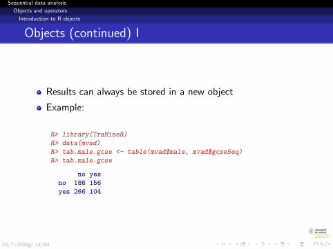
Results can always be stored in a new object

Example:

R> library(TraMineR)

R> data(mvad)

R> tab.male.gcse <- table(mvad$male, mvad$gcse5eq)

R> tab.male.gcse

no yes

no 186 156

yes 266 104

23/7/2009gr 14/64




Objects (continued)

Depending of its class, methods can be directly applied to it

R> plot(tab.male.gcse, cex.axis = 1.5)

tab.male.gcse

no yesno

yes

23/7/2009gr 15/64




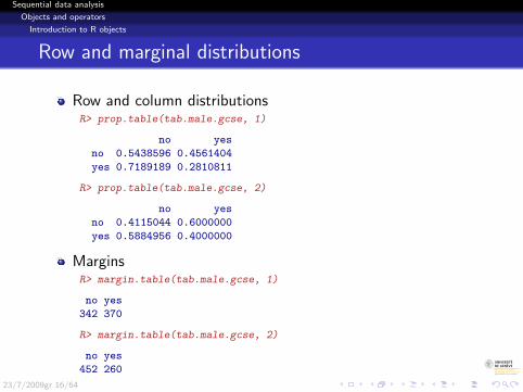
Row and marginal distributions

Row and column distributionsR> prop.table(tab.male.gcse, 1)

no yes

no 0.5438596 0.4561404

yes 0.7189189 0.2810811

R> prop.table(tab.male.gcse, 2)

no yes

no 0.4115044 0.6000000

yes 0.5884956 0.4000000

MarginsR> margin.table(tab.male.gcse, 1)

no yes

342 370

R> margin.table(tab.male.gcse, 2)

no yes

452 260

23/7/2009gr 16/64



Acting on subsets of objects

Section outline


23/7/2009gr 17/64




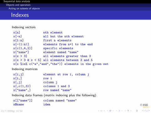
Indexes

Indexing vectors

x[n] nth element

x[-n] all but the nth element

x[1:n] first n elements

x[-(1:n)] elements from n+1 to the end

x[c(1,4,2)] specific elements

x["name"] element named "name"

x[x > 3] all elements greater than 3

x[x > 3 & x < 5] all elements between 3 and 5

x[x %in% c("a","and","the")] elements in the given set

Indexing matrices

x[i,j] element at row i, column j

x[i,] row i

x[,j] column j

x[,c(1,3)] columns 1 and 3

x["name",] row named "name"

Indexing data frames (matrix indexing plus the following)

x[["name"]] column named "name"

x$name idem

23/7/2009gr 18/64




Crosstable on data subsets

Cross tables for catholic and non catholic

R> table(mvad$male[mvad$catholic == "yes"], mvad$gcse5eq[mvad$catholic ==

+ "yes"])

no yes

no 82 77

yes 133 52

R> table(mvad$male[mvad$catholic == "no"], mvad$gcse5eq[mvad$catholic ==

+ "no"])

no yes

no 104 79

yes 133 52

23/7/2009gr 19/64




3-dimensional crosstables

AlternativelyR> table(mvad$male, mvad$gcse5eq, mvad$catholic)

, , = no

no yes

no 104 79

yes 133 52

, , = yes

no yes

no 82 77

yes 133 52

23/7/2009gr 20/64



Importation/exportation

Section outline


23/7/2009gr 21/64




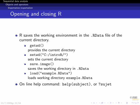
Opening and closing R

R saves the working environment in the .RData file of thecurrent directory.

getwd()provides the current directorysetwd("C:/introR/")

sets the current directorysave.image()

saves the working directory in .RDataload("example.RData")

loads working directory example.RData

On line help command: help(subject), or ?sujet

23/7/2009gr 22/64




Object Management

List of objects in the “Workingspace”R> ls()

[1] "a" "datadir" "filename" "graphdir"

[5] "mvad" "pngdir" "sex" "sex.fac"

[9] "sex.fac2" "sex.fac2n" "tab.male.gcse"

Removing objectsR> rm(sex, sex.fac2)

R> ls()

[1] "a" "datadir" "filename" "graphdir"

[5] "mvad" "pngdir" "sex.fac" "sex.fac2n"

[9] "tab.male.gcse"

23/7/2009gr 23/64




Importing text files

R can import text files (tab-delimited, CSV, ...) withread.table()

read.table(file, header = FALSE, sep = "", quote = "\"'", dec = ".",

row.names, col.names, as.is = FALSE, na.strings = "NA",

colClasses = NA, nrows = -1,

skip = 0, check.names = TRUE, fill = !blank.lines.skip,

strip.white = FALSE, blank.lines.skip = TRUE,

comment.char = "#")

Ex: importing a tab-delimited file with variables names in first row:

R> example <- read.table(file = "example.dat", header = TRUE,

+ sep = "\t")

R> example

age revenu sexe

1 25 100 homme

2 45 200 femme

3 30 50 homme

23/7/2009gr 24/64




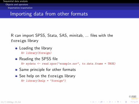
Importing data from other formats

R can import SPSS, Stata, SAS, minitab, ... files with theforeign library

Loading the libraryR> library(foreign)

Reading the SPSS fileR> mydata <- read.spss("example.sav", to.data.frame = TRUE)

Same principle for other formats

See help on the foreign libraryR> library(help = "foreign")

23/7/2009gr 25/64




Exportation

Exporting in text fileR> write.table(mydata, file = "export.txt", sep = "\t")

Labels are lost, factors are saved as strings

Alternatively with foreignR> write.foreign(mydata, datafile = "export.txt",

+ codefile = "export.sps", package = "SPSS")

23/7/2009gr 26/64


Elements of statistical modeling

Outline

1 Introduction






23/7/2009gr 27/64



Statistical modeling: Regression

We use the mvad data of TraMineR

Regression of longitudinal entropies on

male, catholic, ...

23/7/2009gr 28/64



Loading the data

R> mvad.lab <- seqstatl(mvad[, 17:86])

R> mvad.shortlab <- c("EM", "FE", "HE", "JL", "SC", "TR")

R> mvad.seq <- seqdef(mvad[, 17:86], labels = mvad.lab,

+ states = mvad.shortlab)

R> summary(mvad.seq)

[>] dimensionality of the sequence space: 350

[>] 712 sequences in the data set

[>] 490 unique sequences in the data set

[>] min/max sequence length: 70 / 70

[>] alphabet: 1=EM 2=FE 3=HE 4=JL 5=SC 6=TR

[>] colors: 1=#7FC97F 2=#BEAED4 3=#FDC086 4=#FFFF99 5=#386CB0 6=#F0027F

[>] labels: 1=employment 2=FE 3=HE 4=joblessness 5=school 6=training

[>] code for missing statuses: *

[>] code for void state: *

23/7/2009gr 29/64



Computing longitudinal entropies

Computing entropiesR> entrop <- seqient(mvad.seq)

Boxplot of their distributionR> boxplot(entrop, col = "lightblue", cex.axis = 1.5)

●●●●●●●●●●●●●●●●●●●●●●●●●●●●●●●●●●●●●●●●●●●●●●●●●●●●0.0

0.2

0.4

0.6

0.8

23/7/2009gr 30/64



Linear regression: lm() I

Creating the regression objectR> lm.entrop <- lm(entrop ~ male + catholic + gcse5eq, data = mvad)

23/7/2009gr 31/64



Linear regression: results

Displaying the resultsR> summary(lm.entrop)

Call:

lm(formula = entrop ~ male + catholic + gcse5eq, data = mvad)

Residuals:

Min 1Q Median 3Q Max

-4.713e-01 -9.506e-02 2.750e-05 1.286e-01 4.479e-01

Coefficients:

Estimate Std. Error t value Pr(>|t|)

(Intercept) 0.38916 0.01277 30.482 < 2e-16 ***

maleyes -0.04177 0.01329 -3.143 0.00174 **

catholicyes 0.01768 0.01307 1.353 0.17643

gcse5eqyes 0.06451 0.01378 4.680 3.43e-06 ***

---

Signif. codes: 0 '***' 0.001 '**' 0.01 '*' 0.05 '.' 0.1 ' ' 1

Residual standard error: 0.1741 on 708 degrees of freedom

Multiple R-squared: 0.05376, Adjusted R-squared: 0.04975

F-statistic: 13.41 on 3 and 708 DF, p-value: 1.615e-0823/7/2009gr 32/64



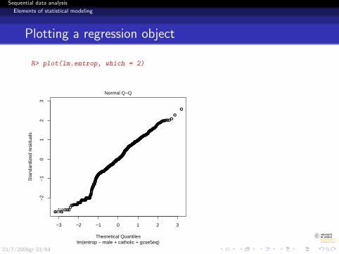
Plotting a regression object

R> plot(lm.entrop, which = 2)

●

●

●

●

●

●

●

●●

●●●

●●

●

●●

●

●

●

●

●

●

●

●

●

●

●●

●

●

●

●

●●

●

●●

●

●

●

●

●●●

●●

●●●●

●

●

●●

●

●

●●

●●

●

●

●

●

●

●

●

●

●

●

●●

●●

●

●

●

●

●

●

●

●●

●

●

●

●

●

●

●

●●

●

●

●

●

●

●

●

●

●

●

●

●

●

●

●

●

●●●

●

●

●

●

●●

●

●

●

●

●●

●●

●

●

●●

●

●

●

●

●

●

●

●●

●

●

●

●

●

●

●

●

●

●

●

●

●

●

●

●

●●

●

●

●●

●

●

●

●

●

●

●

●

●

●

●

●●

●

●

●

●

●

●

●

●

●

●

●

●

●

●

●

●

●

●

●

●

●

●

●

●●

●

●●

●

●

●

●

●●●

●●

●

●

●

●

●●●

●

●

●

●

●●

●

●

●

●

●

●

●

●

●

●

●

●

●

●

●

●

●

●

●

●

●

●

●

●

●●

●●

●

●

●

●

●

●

●

●

●

●

●

●

●

●

●

●

●

●

●

●

●

●

●

●●

●

●

●

●

●

●

●●

●

●●

●

●

●

●

●

●●

●

●

●

●

●

●

●

●

●●

●

●

●

●

●

●

●●

●

●

●●●

●

●

●

●

●

●

●

●●

●

●

●●

●

●

●●

●

●

●

●

●

●

●●

●

●

●●

●

●

●

●

●●

●

●

●

●●●

●

●

●

●

●

●●

●

●

●

●

●

●

●

●

●

●●

●

●

●

●

●

●

●

●

●

●

●

●●

●

●

●

●

●

●

●

●

●

●

●

●

●

●

●

●

●

●

●

●●

●

●

●

●

●

●

●●

●

●

●

●

●●

●

●●

●

●

●

●

●

●

●●

●●

●

●

●

●

●

●

●

●

●

●

●

●

●

●

●

●

●

●

●

●

●

●

●

●

●

●

●

●

●

●

●

●●

●

●

●

●

●

●

●

●

●

●

●

●

●●

●

●

●

●

●

●

●

●

●●

●

●

●

●

●

●

●●

●

●●

●

●

●●

●

●

●

●

●

●

●

●

●

●

●

●

●

●

●

●

●●

●

●

●

●

●●●

●

●

●●

●

●

●

●

●

●

●

●●

●

●

●

●●

●

●

●

●

●

●

●

●

●

●

●●

●

●

●

●

●

●

●●

●

●

●

●

●

●

●

●

●●

●

●

●

●●

●●

●●

●

●●

●

●

●

●

●

●

●

●●●

●

●

●

●

●

●

●

●

●

●

●

●

●

●

●

●

●

●

●

●

●

●

●

●

●

●

●

●

●●

●

●

●

●

●

●

●

●

●

●●

●

●

●

●

●

●

●

●

●

●

●

●

●

●

●

●

●

●

●

●

●●

●

● ●

●

●●

●

●

●

●

●

●

●

●

●

●

●

●

●

●

●

●●

●

●

●

●

●

●

●●

●●

●

●

●

●

●●

●

●

●

●

●

−3 −2 −1 0 1 2 3

−2

−1

01

23

Theoretical Quantiles

Sta

ndar

dize

d re

sidu

als

lm(entrop ~ male + catholic + gcse5eq)

Normal Q−Q

193421310

23/7/2009gr 33/64



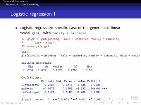
Logistic regression I

Logistic regression: specific case of the generalized linearmodel glm() with family = binomial

R> lg.gr <- glm(gcse5eq ~ male + catholic, family = binomial,

+ data = mvad)

R> summary(lg.gr)

Call:

glm(formula = gcse5eq ~ male + catholic, family = binomial, data = mvad)

Deviance Residuals:

Min 1Q Median 3Q Max

-1.1286 -1.0821 -0.7929 1.2758 1.6189

Coefficients:

Estimate Std. Error z value Pr(>|z|)

(Intercept) -0.2283 0.1315 -1.736 0.0825 .

maleyes -0.7677 0.1588 -4.833 1.34e-06 ***

catholicyes 0.1124 0.1586 0.709 0.4783

---

Signif. codes: 0 '***' 0.001 '**' 0.01 '*' 0.05 '.' 0.1 ' ' 123/7/2009gr 34/64



Logistic regression II

(Dispersion parameter for binomial family taken to be 1)

Null deviance: 934.62 on 711 degrees of freedom

Residual deviance: 910.51 on 709 degrees of freedom

AIC: 916.51

Number of Fisher Scoring iterations: 4

23/7/2009gr 35/64



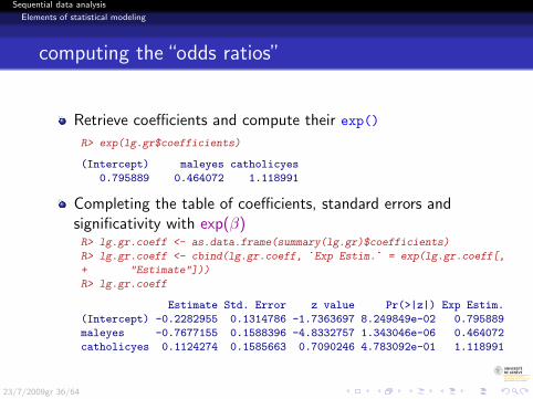
computing the “odds ratios”

Retrieve coefficients and compute their exp()

R> exp(lg.gr$coefficients)

(Intercept) maleyes catholicyes

0.795889 0.464072 1.118991

Completing the table of coefficients, standard errors andsignificativity with exp(β)R> lg.gr.coeff <- as.data.frame(summary(lg.gr)$coefficients)

R> lg.gr.coeff <- cbind(lg.gr.coeff, `Exp Estim.` = exp(lg.gr.coeff[,

+ "Estimate"]))

R> lg.gr.coeff

Estimate Std. Error z value Pr(>|z|) Exp Estim.

(Intercept) -0.2282955 0.1314786 -1.7363697 8.249849e-02 0.795889

maleyes -0.7677155 0.1588396 -4.8332757 1.343046e-06 0.464072

catholicyes 0.1124274 0.1585663 0.7090246 4.783092e-01 1.118991

23/7/2009gr 36/64



ANOVA

ANOVAR> summary(aov(entrop ~ male, data = mvad))

Df Sum Sq Mean Sq F value Pr(>F)

male 1 0.4888 0.4888 15.645 8.406e-05 ***

Residuals 710 22.1807 0.0312

---

Signif. codes: 0 '***' 0.001 '**' 0.01 '*' 0.05 '.' 0.1 ' ' 1

R> summary(aov(lm.entrop))

Df Sum Sq Mean Sq F value Pr(>F)

male 1 0.4888 0.4888 16.1322 6.539e-05 ***

catholic 1 0.0662 0.0662 2.1847 0.1398

gcse5eq 1 0.6637 0.6637 21.9046 3.434e-06 ***

Residuals 708 21.4508 0.0303

---

Signif. codes: 0 '***' 0.001 '**' 0.01 '*' 0.05 '.' 0.1 ' ' 1

23/7/2009gr 37/64


Growing trees: rpart and party

Outline

1 Introduction






23/7/2009gr 38/64



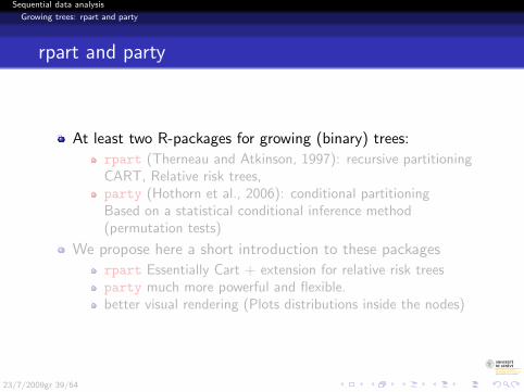
rpart and party

At least two R-packages for growing (binary) trees:

rpart (Therneau and Atkinson, 1997): recursive partitioningCART, Relative risk trees,party (Hothorn et al., 2006): conditional partitioningBased on a statistical conditional inference method(permutation tests)

We propose here a short introduction to these packages

rpart Essentially Cart + extension for relative risk treesparty much more powerful and flexible.better visual rendering (Plots distributions inside the nodes)

23/7/2009gr 39/64



rpart: methods

rpart proposes several methods:

"poisson", rate tree, for binary responses."class", classification tree, when response is a factor."anova", regression tree, when response is quantitative."exp", risk tree, for a survival response.

If method is not specified, rpart tries a guess from theresponse type.

23/7/2009gr 40/64



rpart

Section outline

5 Growing trees: rpart and partyrpartparty

23/7/2009gr 41/64



rpart

Growing a rate tree rpart

R> library(rpart)

R> cart.mvad.gcse <- rpart(gcse5eq ~ male + catholic, data = mvad,

+ method = "poisson", control = list(minsplit = 20,

+ minbucket = 10, cp = 1e-04))

R> cart.mvad.gcse

n= 712

node), split, n, deviance, yval

* denotes terminal node

1) root 712 115.74880 1.365169

2) male=yes 370 53.52554 1.281247 *

3) male=no 342 58.23767 1.455946

6) catholic=no 183 30.99274 1.431429 *

7) catholic=yes 159 27.08354 1.483731 *

23/7/2009gr 42/64



rpart

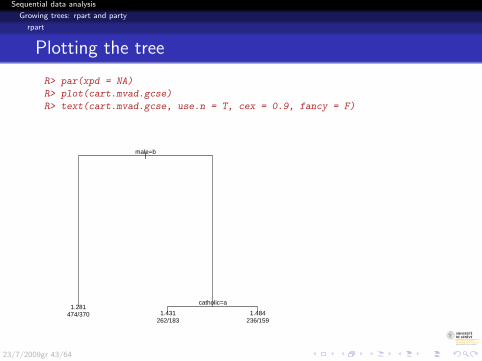
Plotting the tree

R> par(xpd = NA)

R> plot(cart.mvad.gcse)

R> text(cart.mvad.gcse, use.n = T, cex = 0.9, fancy = F)

|male=b

catholic=a1.281

474/370 1.431262/183

1.484236/159

23/7/2009gr 43/64



rpart

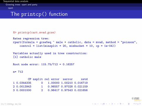
The printcp() function

R> printcp(cart.mvad.gcse)

Rates regression tree:

rpart(formula = gcse5eq ~ male + catholic, data = mvad, method = "poisson",

control = list(minsplit = 20, minbucket = 10, cp = 1e-04))

Variables actually used in tree construction:

[1] catholic male

Root node error: 115.75/712 = 0.16257

n= 712

CP nsplit rel error xerror xstd

1 0.0344335 0 1.00000 1.00210 0.016719

2 0.0013943 1 0.96557 0.97028 0.021159

3 0.0001000 2 0.96417 0.97543 0.021656

23/7/2009gr 44/64



rpart

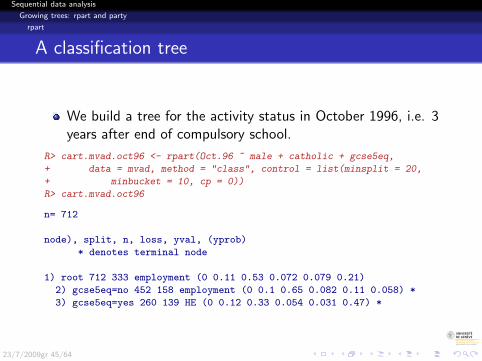
A classification tree

We build a tree for the activity status in October 1996, i.e. 3years after end of compulsory school.

R> cart.mvad.oct96 <- rpart(Oct.96 ~ male + catholic + gcse5eq,

+ data = mvad, method = "class", control = list(minsplit = 20,

+ minbucket = 10, cp = 0))

R> cart.mvad.oct96

n= 712

node), split, n, loss, yval, (yprob)


1) root 712 333 employment (0 0.11 0.53 0.072 0.079 0.21)

2) gcse5eq=no 452 158 employment (0 0.1 0.65 0.082 0.11 0.058) *

3) gcse5eq=yes 260 139 HE (0 0.12 0.33 0.054 0.031 0.47) *

23/7/2009gr 45/64



rpart

survival risk tree

We build a survival data object for time to marriage from thebiofam data set provided with TraMineR

States of interest are:

2: married without leaving home3: married and left home6: married with child7: divorced

If divorce occurs before any marriage, we assume marriage anddivorce the same year.

23/7/2009gr 46/64



rpart

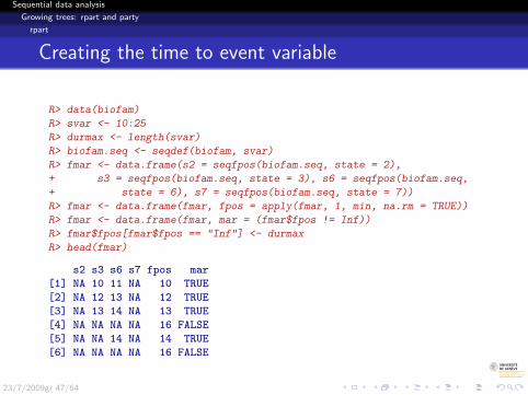
Creating the time to event variable

R> data(biofam)

R> svar <- 10:25

R> durmax <- length(svar)

R> biofam.seq <- seqdef(biofam, svar)

R> fmar <- data.frame(s2 = seqfpos(biofam.seq, state = 2),

+ s3 = seqfpos(biofam.seq, state = 3), s6 = seqfpos(biofam.seq,

+ state = 6), s7 = seqfpos(biofam.seq, state = 7))

R> fmar <- data.frame(fmar, fpos = apply(fmar, 1, min, na.rm = TRUE))

R> fmar <- data.frame(fmar, mar = (fmar$fpos != Inf))

R> fmar$fpos[fmar$fpos == "Inf"] <- durmax

R> head(fmar)

s2 s3 s6 s7 fpos mar

[1] NA 10 11 NA 10 TRUE

[2] NA 12 13 NA 12 TRUE

[3] NA 13 14 NA 13 TRUE

[4] NA NA NA NA 16 FALSE

[5] NA NA 14 NA 14 TRUE

[6] NA NA NA NA 16 FALSE

23/7/2009gr 47/64



rpart

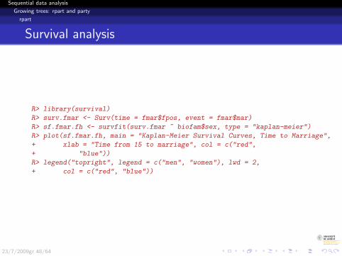
Survival analysis

R> library(survival)

R> surv.fmar <- Surv(time = fmar$fpos, event = fmar$mar)

R> sf.fmar.fh <- survfit(surv.fmar ~ biofam$sex, type = "kaplan-meier")

R> plot(sf.fmar.fh, main = "Kaplan-Meier Survival Curves, Time to Marriage",

+ xlab = "Time from 15 to marriage", col = c("red",

+ "blue"))

R> legend("topright", legend = c("men", "women"), lwd = 2,

+ col = c("red", "blue"))

23/7/2009gr 48/64



rpart

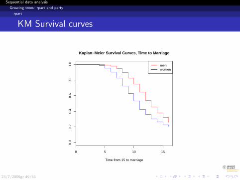
KM Survival curves

0 5 10 15

0.0

0.2

0.4

0.6

0.8

1.0

Kaplan−Meier Survival Curves, Time to Marriage

Time from 15 to marriage

menwomen

23/7/2009gr 49/64



rpart

Covariates

Preparing covariatesR> coho1 <- factor(biofam$birthyr < 1940)

R> coho2 <- factor(biofam$birthyr >= 1940 & biofam$birthyr <

+ 1950)

R> coho3 <- factor(biofam$birthyr >= 1950)

R> lang <- biofam$plingu02

R> sex <- biofam$sex

R> covariates <- data.frame(sex, lang, coho1, coho2, coho3)

R> head(covariates)

sex lang coho1 coho2 coho3

1 man german FALSE TRUE FALSE

2 man german TRUE FALSE FALSE

3 woman french FALSE TRUE FALSE

4 man german TRUE FALSE FALSE

5 man german FALSE TRUE FALSE

6 man italian TRUE FALSE FALSE

23/7/2009gr 50/64



rpart

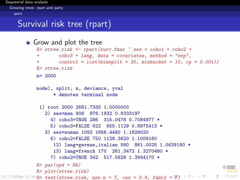
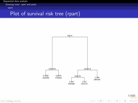
Survival risk tree (rpart)

Grow and plot the treeR> stree.risk <- rpart(surv.fmar ~ sex + coho1 + coho2 +

+ coho3 + lang, data = covariates, method = "exp",

+ control = list(minsplit = 20, minbucket = 10, cp = 0.001))

R> stree.risk

n= 2000

node), split, n, deviance, yval


1) root 2000 2681.7330 1.0000000

2) sex=man 908 978.1932 0.8333197

4) coho3=TRUE 286 315.0478 0.7084977 *

5) coho3=FALSE 622 655.1129 0.8975413 *

3) sex=woman 1092 1656.4480 1.1828020

6) coho2=FALSE 750 1128.3620 1.1009180

12) lang=german,italian 580 861.0025 1.0439180 *

13) lang=french 170 261.3472 1.3270480 *

7) coho2=TRUE 342 517.5828 1.3944170 *

R> par(xpd = NA)

R> plot(stree.risk)

R> text(stree.risk, use.n = T, cex = 0.9, fancy = F)23/7/2009gr 51/64



rpart

Plot of survival risk tree (rpart)

|sex=a

coho3=b coho2=a

lang=bc0.7085193/286

0.8975479/622

1.044444/580

1.327141/170

1.394285/342

23/7/2009gr 52/64



party

Section outline

5 Growing trees: rpart and partyrpartparty

23/7/2009gr 53/64



party

party principle

party selects each split in two steps (to avoid bias in favor ofpredictors with many different values):

First, selects the predictor with strongest association withtarget,Then, selects the best binary split for selected predictor.

23/7/2009gr 54/64



party

Linear statistic and permutation test

Both steps are based on the conditional distribution of linearstatistics in a permutation test framework.

Linear statistic is:

Tj = vec( n∑

i=1

wigj(Xji )h(Yi , (Y1, . . . ,Yn)

)T) ∈ Rpjq

where gj(Xji ) is a transformation of Xji , and h() an influencefunction.Tj is computed for each permutation of the Y values amongcases, and results characterize its conditional independencedistribution.the variable and split selection is then based on the p-value ofthe observed t under this conditional independence distribution.

23/7/2009gr 55/64



party

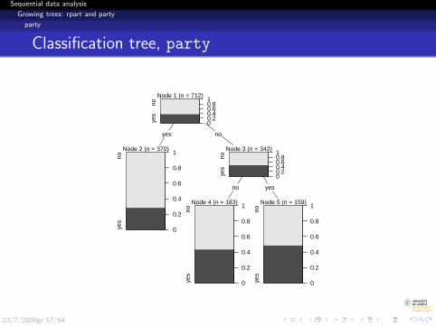
A R script for generating a tree

You grow the tree with the ctree command

R> library(party)

R> ctree.mvad.gcse <- ctree(gcse5eq ~ male + catholic, data = mvad,

+ controls = ctree_control(mincriterion = 0.3, minsplit = 0),

+ )

R> plot(ctree.mvad.gcse, drop_terminal = F, inner_panel = node_barplot)

23/7/2009gr 56/64



party

Classification tree, party

Node 1 (n = 712)

yes

no

00.20.40.60.81

yes no

Node 2 (n = 370)

yes

no

0

0.2

0.4

0.6

0.8

1Node 3 (n = 342)

yes

no

00.20.40.60.81

no yes

Node 4 (n = 183)

yes

no

0

0.2

0.4

0.6

0.8

1Node 5 (n = 159)

yes

no

0

0.2

0.4

0.6

0.8

1

23/7/2009gr 57/64



party

Classification tree, text output, party

R> ctree.mvad.gcse

Conditional inference tree with 3 terminal nodes

Response: gcse5eq

Inputs: male, catholic

Number of observations: 712

1) male == {yes}; criterion = 1, statistic = 23.462

2)* weights = 370

1) male == {no}

3) catholic == {no}; criterion = 0.448, statistic = 0.945

4)* weights = 183

3) catholic == {yes}

5)* weights = 159

23/7/2009gr 58/64



party

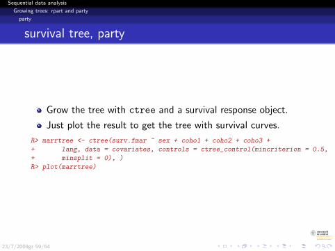
survival tree, party

Grow the tree with ctree and a survival response object.

Just plot the result to get the tree with survival curves.

R> marrtree <- ctree(surv.fmar ~ sex + coho1 + coho2 + coho3 +

+ lang, data = covariates, controls = ctree_control(mincriterion = 0.5,

+ minsplit = 0), )

R> plot(marrtree)

23/7/2009gr 59/64



party

Survival tree, text output, party

R> marrtree

Conditional inference tree with 5 terminal nodes

Response: surv.fmar

Inputs: sex, coho1, coho2, coho3, lang

Number of observations: 2000

1) sex == {woman}; criterion = 1, statistic = 54.008

2) coho2 == {TRUE}; criterion = 0.989, statistic = 9.395

3)* weights = 342

2) coho2 == {FALSE}

4) lang == {french}; criterion = 0.862, statistic = 7.067

5)* weights = 170

4) lang == {german, italian}

6)* weights = 580

1) sex == {man}

7) coho3 == {FALSE}; criterion = 0.996, statistic = 11.284

8)* weights = 622

7) coho3 == {TRUE}

9)* weights = 286

23/7/2009gr 60/64



party

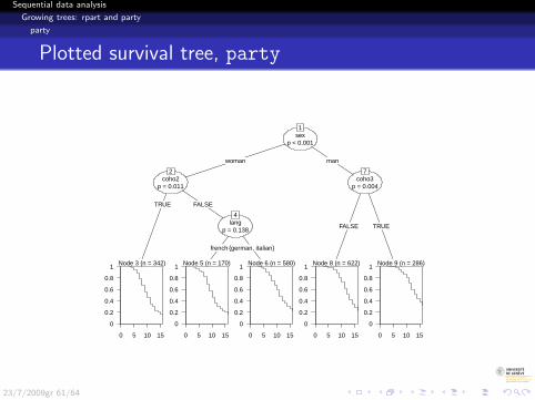
Plotted survival tree, party

sexp < 0.001

1

woman man

coho2p = 0.011

2

TRUE FALSE

Node 3 (n = 342)

0 5 10 15

0

0.2

0.4

0.6

0.8

1

langp = 0.138

4

french {german, italian}

Node 5 (n = 170)

0 5 10 15

0

0.2

0.4

0.6

0.8

1Node 6 (n = 580)

0 5 10 15

0

0.2

0.4

0.6

0.8

1

coho3p = 0.004

7

FALSE TRUE

Node 8 (n = 622)

0 5 10 15

0

0.2

0.4

0.6

0.8

1Node 9 (n = 286)

0 5 10 15

0

0.2

0.4

0.6

0.8

1

23/7/2009gr 61/64


Custom functions and programming

Outline

1 Introduction






23/7/2009gr 62/64



Functions

R> discretize <- function(a) {

+ if (a < 0.4) {

+ return(1)

+ }

+ else {

+ if (a < 0.6) {

+ return(2)

+ }

+ else {

+ return(3)

+ }

+ }

+ }

R> discretize(0.33)

[1] 1

R> table(apply(entrop, 1, discretize))

1 2 3

385 243 84

23/7/2009gr 63/64



References I

Gabadinho, A., G. Ritschard, M. Studer, and N. S. Muller (2008). Miningsequence data in R with TraMineR: A user’s guide. Technical report,Department of Econometrics and Laboratory of Demography, University ofGeneva, Geneva. (TraMineR is on CRAN the Comprehensive R ArchiveNetwork).

Hothorn, T., K. Hornik, and A. Zeileis (2006). party: A laboratory for recursivepart(y)itioning. User’s manual.

Maindonald, J. and J. Brown (2006). Data Analysis and Graphics Using R: AnExample-based Approach. Cambridge Series in Statistical and ProbabilisticMathematics. Cambridge: Cambridge University Press.

Paradis, E. (2006). R for beginners. Manual, Institut des Sciences de l’Evolution, Universite Montpellier II.

R-Development-Core-Team (2008). An introduction to R (v 2.8.0). Manual,R-project.

Spector, P. (2008). Data Manipulation with R. New York: Springer.

Therneau, T. M. and E. J. Atkinson (1997). An introduction to recursivepartitioning using the rpart routines. Technical Report Series 61, MayoClinic, Section of Statistics, Rochester, Minnesota.23/7/2009gr 64/64

Sequential data analysis An introduction to R -...

Documents

Transcript of Sequential data analysis An introduction to R -...