Sequential Bargaining in the Field: Evidence from...

Sequential Bargaining in the Field: Evidence from

Millions of Online Bargaining Interactions∗

Matthew Backus† Thomas Blake‡ Brad Larsen§ Steven Tadelis¶

March 8, 2018

Abstract

We study patterns of behavior in bilateral bargaining situations using a rich, new dataset

describing over 88 million listings from eBay’s Best Offer platform, with back-and-forth

bargaining occurring in over 25 million of these listings. We document patterns of behavior

and relate them to “rational” and “psychological” theories of bargaining and find that

bargaining patterns are consistent with elements of both approaches. Most notably, players

with more bargaining strength typically receive better outcomes, and players exhibit equi-

table behavior by making offers that split-the-difference between negotiating positions. We

are publicly releasing this new dataset to support additional empirical bargaining research.

JEL classifications: C78, D82, D83, M21.

∗We are grateful to eBay for allowing us to make the data used herein accessible and publicly available.We thank Luis Cabral, Peter Cramton, Emin Karagozoglu, Saul Lach, and Axel Ockenfels for thoughtfulcomments. We thank Brenden Eum, Ziao Ju, Rebecca Li, and Caio Waisman for outstanding researchassistance. Part of this research was supported by NSF Grant SES-1629060.†Columbia University and NBER, [email protected]‡eBay Research, [email protected]§Stanford University and NBER; [email protected]¶UC Berkeley, NBER, CEPR, and CESifo, [email protected]

1 Introduction

Bilateral bargaining is one of the oldest and most common forms of trade. Nations

negotiate trade deals, arms control, and climate change mitigation; legislators engage

in horse-trading to build coalitions and pass legislation; business people haggle over

contracts from corporate acquisitions to labor agreements; lawyers wrangle settlements

both civil and criminal, and private individuals bargain over wages, real estate, and the

allocation of household chores. Bargaining determines the allocation of surplus in these

settings, as well as the likelihood of breakdown—the latter with real economic and

human costs. Therefore, understanding how people bargain, and the institutions, norms,

and practices that affect bargaining outcomes, is a question of first-order importance.

Over the past sixty years, a large literature in economics has examined various

aspects of bargaining in theory and in laboratory experiments, but little evidence has

been presented about how people bargain in the field, and how negotiated prices

actually form in real-world negotiations. The theoretical literature typically assumes

a particular information structure and extensive form of the game, while bargaining

in real-world settings tends to be less structured. The advent of online marketplaces

provides a new opportunity to study negotiations in a setting where the extensive form

of the game is similar to those studied in the theoretical and experimental literature, but

with the advantage of being a setting where real-live participants are negotiating and

where the data collection is on a massive scale. In this paper, we utilize data on over

88 million listings on the eBay.com “Best Offer” platform, where sellers offer items at

a listed price and invite buyers to engage in alternating, sequential-offer bargaining,

very much in the spirit of Rubinstein (1982). In over 25 million of these listings, buyers

chose to make an offer, initiating the alternating-offer game. Within this setting, we

document a variety of facts on how bargaining proceeds and how prices form and the

forces that play a role in this process. We find evidence consistent with the most salient

predictions of economic theory and also document evidence suggesting that behavioral

factors based on equitable norms play a significant role in bargaining outcomes.

Our data come from eBay’s Best Offer platform. While more widely known for its

sales of goods through auctions or a fixed price, eBay has also offered sales through

alternating-offer bargaining for over a decade, and now almost ten percent of eBay

transaction volume occurs through bargaining. The mechanism allows each player in a

1

given buyer-seller pair to make up to three offers each. Given the sheer volume of trade

on eBay and the simple extensive form of the game, the Best Offer platform provides

a useful setting for studying the determination of agreed-upon prices in sequential

bargaining situations.1 The bargaining in this setting is only over a single dimension

(price), making it more straightforward to analyze than many other bargaining settings

(such as procurement contracts; Bajari et al. 2009), while still yielding the benefit of

being a real-world setting. Furthermore, the data allows us to link buyers and sellers

over time.

This dataset is, to our knowledge, the largest offer-level negotiations dataset to be

analyzed in the literature. In cooperation with eBay, we have anonymized the dataset

and have been given clearance to make it publicly available for research purposes. The

data can be accessed at http://www.nber.org/data/bargaining.html or by contacting

the authors. We hope that it will further fuel the recent surge of empirical work studying

bargaining in economics and stimulate additional work in the area, both empirical and

theoretical.

After summarizing recent work in the growing empirical bargaining literature in

Section 2, Section 3 describes background on the Best Offer platform and introduces our

dataset. Section 4 then documents how patterns observed in the data relate to rational

game-theoretic theories of bargaining. We provide a breakdown of how bargaining

sequences unfold in practice and the frequency with which different responses and

outcomes occur. We find that there are typically few back-and-forth offers between a

given bargaining pair, which is consistent with complete-information, common-priors

models of bargaining, such as the classical Rubinstein (1982) model. However, the fact

that some delay in agreement is observed is consistent with models of heterogeneous

priors (Yildiz 2003) or incomplete information (Rubinstein 1985; Admati and Perry

1987; Cramton 1992). And the observation that bargaining very frequently ends in

disagreement is consistent with the presence of incomplete information and bargaining

1Fudenberg et al. (1985) explained that the “thorny issue” arising in much of the bargaining literatureis that the researcher does not actually know the extensive form of real-world bargaining scenarios. Forexample, a street vendor bargaining over price might state an offer, watch the facial reaction of the buyer,and immediately state a lower price without waiting for a spoken response by the buyer. It is unclearwhether this situation should be modeled with alternating offers, one-sided offers, a concession game, orany number of possible options. In the situation we study, the extensive form is much clearer: buyers andsellers participate in an alternating-offer bargaining game through eBay’s platform, and never interactwith one another except through this platform.

2

costs. We show that the character of bargaining is different when players bargain over

expensive versus inexpensive products, in a way that is consistent with fixed costs of

bargaining playing a role.

We also find that final prices form very quickly, although not instantaneously, and

these final prices tend to be well within the interior of initial offers. We find that prices

tend to converge in a pattern consistent with Coasian dynamics, with seller offers

declining and buyer offers increasing over the duration of the bargaining interaction.

We demonstrate that bargaining sequences that end through the seller declining after

several back-and-forth offers are likely to be interactions in which the seller budged

little even from the initial listing price, while we do not find this result for buyers.

We also demonstrate that, for used goods, variation in the features of the bargaining

sequence—namely, whether the bargaining is successful, the number of offers made in

the bargaining sequence, and the final price—can be explained more by heterogeneity

in the participating buyer than by heterogeneity in the seller or in the product itself.

With new goods, on the other hand, variance in the final negotiated prices is explained

equally well by player heterogeneity and by product heterogeneity.

We examine several forms of bargaining strength. We find that buyers who are

more patient (as measured by their ex-post choice of shipping speed) tend to obtain

lower prices in the bargaining. Buyers who are more experienced in bargaining on this

platform (as measured by the number of previous Best Offer negotiations the buyer has

participated in) also tend to achieve lower final prices, and experienced sellers achieve

higher final prices. These results are consistent with common models of bargaining

in which patience or other measures of a player’s bargaining power affect outcomes

(Rubinstein 1982, 1985; Watson 1998); they are also consistent with laboratory evidence

(Rapoport et al. 1995) and survey data (Scott Morton et al. 2011), but, to our knowledge,

have not been previously confirmed with data from actual bargaining outcomes.

In Section 5 we explore players’ choices of counteroffers. We find that participants

in the market appear to concede more to the opposing party when the opposing party

is more experienced and concede less when they themselves are more experienced.

We also analyze aspects of non-standard, or “behavioral” bargaining models by ex-

amining the phenomenon documented throughout the experimental and theoretical

behavioral literature that market participants care about fairness, and often favor a

3

split-the-difference strategy in bargaining (Roth and Malouf 1979; Roth 1985; Binmore

et al. 1985; Bolton 1991; Bolton and Ockenfels 2000; Charness and Rabin 2002; An-

dreoni and Bernheim 2009). We demonstrate that a player often makes offers lying

halfway between the player’s own previous offer and the opponent’s current offer. We

further demonstrate that such split-the-difference offers have a higher likelihood of

being accepted—higher even than some offers that would be even more favorable in

money terms for the accepting party. This is consistent with preferences for fairness as

symmetry, notably with endogenous reference points.

While similar results have been documented among laboratory participants, these

are the first results of which we are aware documenting such findings in a real-world

setting. The large scale of our data and the variation across several measures of het-

erogeneity help paint a useful picture of sequential bargaining in the real world, and

confirm some of the most basic insights of bargaining theory.

2 Recent Empirical Work on Bargaining

Until recently, there was limited empirical work corresponding to the sprawling theoret-

ical literature on bargaining in economics. That work was mostly confined to the study

of labor negotiations and strikes (see, e.g., Cramton and Tracy 2003). The past five years,

however, have seen a burst of empirical studies of bargaining due to two concurrent

events: first, the development of tractable empirical models of bargaining for the study

of price-setting, and second, the increasing availability of data on bargaining outcomes.

Here we offer a map of current empirical work on bargaining based on the underlying

theory.

A commonly applied model of bargaining for empirical work is the cooperative

game theory concept of Nash bargaining, where players choose a price that maximizes

the joint product of their surplus, weighted by the player’s bargaining power weights.2

These models are tractable and offer unique solutions, making them extremely useful

for empirical work. This is particularly true in settings where the only observable

information from a bargaining process is the final price and only for instances when the

2Nash (1950) introduced a parsimonious set of axioms that resulted in a solution with these properties.

4

negotiating parties reach agreement. Early structural work on bargaining made these

assumptions to make otherwise unwieldy settings tractable, e.g. Elyakime et al. (1997).

Horn and Wolinsky (1988) extended the Nash bargaining solution to model vertical

firm-to-firm pricing. Their model softened the take-it-or-leave it assumption of tradi-

tional models of vertical relations, but required a restrictive assumption on disagreement

payoffs: that players do not incorporate the outside option of bargaining with other

parties. This assumption has become known as “Nash-in-Nash,” and noncooperative

underpinnings for this model are explored in Collard-Wexler et al. (2014). The useful-

nesses of the Horn and Wolinsky (1988) model was first exploited in Crawford and

Yurukoglu (2012), who studied the cable industry and demonstrated the importance of

accounting for bargaining in vertical relationships firms when evaluating downstream

retail bundling. Subsequently, the method has been applied to study insurance networks

(Ho and Lee, 2017), bargaining over medical devices (Grennan, 2013), hospital mergers

(Gowrisankaran et al., 2015), and vertical mergers in cable programming (Crawford

et al., 2015), to cite a few leading examples in this growing literature.

Nash bargaining and Nash-in-Nash bargaining, while yielding tractability, neither

explain nor accommodate bargaining breakdown, and the latter framework requires

restrictions on the formulation of disagreement payoffs. This second limitation has

sparked interests in a number of extensions, currently underway, that seek to add an

element of strategic exclusion following the “outside option principle” of Binmore et al.

(1989) (see, for example, Ghili (2016) and Ho and Lee (2016)).

Merlo and Tang (2012) also focus on complete-information settings, but study

stochastic bargaining games in which the size of the surplus may be unknown to

the players. The authors discuss identification and estimation strategies in these settings

and develop an identification strategy for stochastic bargaining games. In later work,

Merlo and Tang (2016) propose and estimate a complete-information model with hetero-

geneous priors, applying their framework to medical malpractice suits. As emphasized

in the theory literature, models of heterogeneous priors can offer explanations of delay

or breakdown that cannot be explained by traditional Nash bargaining.

Unlike the tractability of the Nash bargaining framework, non-cooperative game

theory models of bargaining, which depend on explicit procedures and incorporate

incomplete information, are often plagued by multiple equilibria and unclear predic-

5

tions. Due to these complications, very little empirical work exists viewing bargaining

through a lens of incomplete information. Such work includes several papers apply-

ing structural approaches, including Ambrus et al. (2016), who estimated a one-sided

incomplete-information model that highlighted a signaling role for delay by exploiting

exogenous variation in the time to counteroffers in ransom negotiations with Mediter-

ranean pirates. Silveira (2017) studied identification of asymmetric information models

of bargaining to study sentencing guidelines in pre-trial negotiations. Keniston (2011)

nested sequential-offer bargaining in an empirical dynamic game framework, using

field experimental data from India to study the welfare implications of transacting

through bargaining versus through posted prices. Allen et al. (2014) presented a search

model with bargaining to study the welfare loss due to negotiation frictions in oligopoly

markets. Larsen (2014) and Larsen and Zhang (2017) estimated primitives of two-sided

incomplete-information sequential-offer bargaining games while remaining agnostic

about the bargaining protocol and used these primitives to study bargaining efficiency

and equity in wholesale used-car markets.

Several recent papers have also documented insights from reduced-form analyses

in several bargaining settings. Scott Morton et al. (2011) documented the significance

of search costs and incomplete information in the market for new cars. Grennan and

Swanson (2016) studied the effect of price transparency on bargaining marketplaces,

testing predictions of a model of incomplete information. Shelegia and Sherman (2014)

and Jindal and Newberry (2017) study the costs of bargaining using data on retail

negotiations. Finally, Bagwell et al. (2017) documented a number of data patterns from

negotiated trade agreements, where they observe back-and-forth offers.

Finally, a promising and yet still largely untapped area for empirical work is the

analysis of models that append a “pre-game” to the bargaining protocol. A large set

of theoretical models study these games, which can be used to formalize notions of

pre-commitment a la Schelling (Crawford, 1982), or to capture a role for communication.

The role of communication in bargaining is particularly difficult to assess because it

is “cheap talk,” however there is theoretical and empirical evidence to suggest it may

be important (Farrell and Gibbons, 1989; Radner and Schotter, 1989; Crawford, 1990;

Cabral and Sakovics, 1995; Valley et al., 2002). Two recent papers addressing these issues

are Backus et al. (2016), which documents the use of round numbers as a cheap-talk

signal in bargaining, and Backus et al. (2018), which exploits a natural experiment in

6

Figure 1: Best Offer User Interface

Notes: This figure depicts the “view item” page for a listing with Best Offer enabled. The potential buyer may click on “Buy itNow” to purchase the painting at the listed price of $746.40—or they may click on “Make Offer” and be prompted to propose aprice.

the availability of text communication in Best Offer bargaining on eBay.de to study the

the role of communication in facilitating bargaining.

3 eBay’s Best Offer Mechanism: Facts and Data

eBay is one of the world’s largest online marketplace for consumer-to-consumer transac-

tions. It began in 1995 using second-price-like auctions as the sole format for transacting

on its platform. The site eventually allowed users the option of selling goods through

a single posted fixed-price. In 2005, the site began to allow sellers to sell through an

alternating-offer protocol referred to as “Best Offer.” This feature can be enabled (at

no cost) by the seller at the creation of the listing, and is only available for fixed-price

listings—there is no equivalent mechanism for auctions.

7

Goods offered for sale under the Best Offer format are listed as “accepts Best Offer”

in eBay search results.3 Throughout, we refer to these postings as Best Offer listings. A

buyer viewing a Best Offer listing sees similar information to a buyer viewing a fixed

price listing (referred to as a “Buy It Now” (BIN) listing), including the auction title,

seller id and feedback score, at least one picture of the item, and any other information

about the item that the seller decides to display.4 The buyer sees the BIN price, as in a

standard fixed price listing, but also sees an additional option, a button labeled “Make

Offer”, as illustrated in Figure 1. Selecting the Make Offer button allows the buyer to

send an offer to the seller. As such, we treat the BIN price (equivalently, “listing price”)

as the seller’s first offer to any buyer who wished to bargain.

Upon receiving this offer, the seller may accept the offer, make a counteroffer, or

decline the offer (without making a counteroffer in return).5 If the seller makes a

counteroffer, the buyer then can accept, decline, or counter in response. Play continues

until either party accepts or until the buyer declines. If the seller declines, the buyer may

still respond with a counteroffer or can, at any time, purchase at the BIN price. Each

party is limited to three offers (not including the listing price), and each offer expires 48

hours after being placed.6 We will refer to a sequence of back-and-forth offers —i.e. a

given buyer and seller pair bargaining over a given item — as a thread.

The Best Offer platform is currently a fast-growing sales format on eBay. Figure 2

shows the growth of this format relative to auctions and fixed price listings over the

past ten years. In 2005, when the format was first rolled out, only a tiny fraction of

listings were Best Offer listings, less than 1% of all eBay transactions occurred through

a buyer actually placing an offer (rather than accepting the Buy It Now price). By 2012,

that fraction had grown to just under 9%.

Figure 3 displays the percent of transactions that took place through Best Offer

for each major sales category from 2005–2015. The left panel demonstrates that the

3Potential buyers may filter search results to display only those listings that accept offers.4Throughout, we will use the term “buyer” to refer to the user interested in potentially buying the

item whether or not the transaction actually occurs.5As a time-saving device for sellers, the platform offers sellers the option to specify an “auto-accept”

price which is unobserved to buyers and which, if exceeded by the buyer’s offer, will result in the platformaccepting the offer on behalf of the seller. Seller’s can similarly specify an “auto-decline” price.

6In 2017 this maximum limit was changed to five offers. In our sample, approximately 1.1 percent ofinteractions reach the binding limit, and most of these fail; see Figure 4 below. The limit was extended inan attempt to encourage these negotiators to succeed. The time frame of our data does not permit us toevaluate this policy change.

8

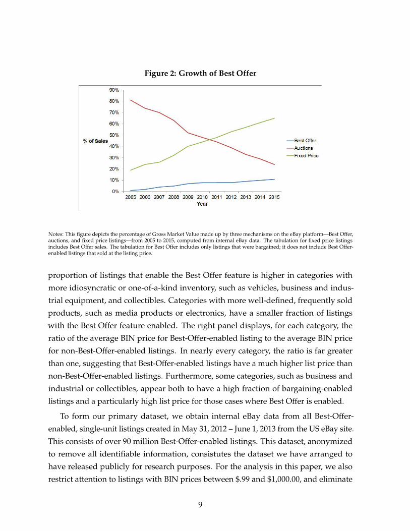
Figure 2: Growth of Best Offer

Notes: This figure depicts the percentage of Gross Market Value made up by three mechanisms on the eBay platform—Best Offer,auctions, and fixed price listings—from 2005 to 2015, computed from internal eBay data. The tabulation for fixed price listingsincludes Best Offer sales. The tabulation for Best Offer includes only listings that were bargained; it does not include Best Offer-enabled listings that sold at the listing price.

proportion of listings that enable the Best Offer feature is higher in categories with

more idiosyncratic or one-of-a-kind inventory, such as vehicles, business and indus-

trial equipment, and collectibles. Categories with more well-defined, frequently sold

products, such as media products or electronics, have a smaller fraction of listings

with the Best Offer feature enabled. The right panel displays, for each category, the

ratio of the average BIN price for Best-Offer-enabled listing to the average BIN price

for non-Best-Offer-enabled listings. In nearly every category, the ratio is far greater

than one, suggesting that Best-Offer-enabled listings have a much higher list price than

non-Best-Offer-enabled listings. Furthermore, some categories, such as business and

industrial or collectibles, appear both to have a high fraction of bargaining-enabled

listings and a particularly high list price for those cases where Best Offer is enabled.

To form our primary dataset, we obtain internal eBay data from all Best-Offer-

enabled, single-unit listings created in May 31, 2012 – June 1, 2013 from the US eBay site.

This consists of over 90 million Best-Offer-enabled listings. This dataset, anonymized

to remove all identifiable information, consistutes the dataset we have arranged to

have released publicly for research purposes. For the analysis in this paper, we also

restrict attention to listings with BIN prices between $.99 and $1,000.00, and eliminate

9

Figure 3: Percent BO Transactions and Ratio of BIN for BO/non-BO by Category

0%

10%

20%

30%

40%

50%

60%

70%

80%

Fraction of Listings with Best Offer Enabled

0.00

2.00

4.00

6.00

8.00

10.00

12.00

Relative BIN Price: BO to non-BO Listings

Notes: Left panel displays, for a number of categories, the proportion of listings with Best Offer enabled. Right panel computes, foreach category, the ratio of the average BIN price for Best-Offer-enabled listing to the average BIN price for non-Best-Offer-enabledlistings.

listings with apparent data errors (e.g., cases where we could not locate the original offer

corresponding to a counteroffer). Details on our sample construction criteria appear in

Appendix B.

Our final dataset analyzed in this paper contains approximately 88.4 million listings.

Of these, 25.4 million received a bargaining offer. Thus, there are 25.4 million bargaining

threads (defined as a listing-buyer pair). These bargaining threads involve 1.2 million

buyers and 4.7 million sellers. The top panel of Table 1 presents descriptive statistics

for this sample. The average list price (BIN) is $95, and the average sale price is 83% of

the list price. Sales include BIN choices as well—conditional on bargaining occurring,

the average sale prices comes down to 73% of the list price. We note that almost 80%

of listings never receive an offer and do not sell. 54.8% of listings are for used goods,

and 26.3% of listings have the BIN price revised at some point by the seller during the

listing life.

Table 1 also includes detailed information on market participants. On average,

sellers have a 99.4% positive feedback score. While there are many one-time sellers,

the market is skewed towards experienced sellers: the average number of listings per

seller is 74, sixteen of which sell, ten of which sell through bargaining. Most of the sales

in our dataset are made by a relatively small fraction of the sellers. The population

of buyers is skewed, but less so: on average, buyers in our sample are observed in 5

10

Table 1: Descriptive Statistics

Mean Std. Dev. Min MaxListing-Level DataListing Price 94.6 164 .01 1,000Used .548 .498 0 1List Price Ever Revised .263 .44 0 1Sold .215 .411 0 1Sold by Best Offer .132 .338 0 1Received an Offer .206 .405 0 1Sale Price 69.7 119 .01 1,000Sale Price / List Price .832 .175 .00099 1Bargained Price 74.1 121 .99 1,000Bargained Price / List Price .727 .146 .00099 1No. Listings 88,388,220Seller-Level DataFeedpack Postitive Percent 99.4 5.3 0 100No. Listings 73.8 1,941 1 1,084,794No. Sales 15.9 158 0 66,989No. Sales by Best Offer 9.72 101 0 56,480No. Sellers 1,197,419Buyer-Level DataNo. Bargaining Threads 5.12 17.9 1 5,697No. Offers 8.48 30 1 7,823No. Purchases 3.21 9.27 1 4,095No. Bargained Purchases 2.47 7.39 0 3,329No. Buyers 4,701,455Thread-Level DataNo. Offers 1.66 .942 1 6Agreement Reached .454 .498 0 1First Buyer Offer 86.6 126 0 1,000First Buyer Offer / List Price .608 .193 0 1No. Threads 25,458,516

Notes: This table presents summary statistics for the main dataset. Note that indicator “Used” (for used vs. new status of item)is only available for 60,709,655 listings, and feedback variables are only available for 1,145,426 sellers. See text for a discussion ofexclusion criteria and, in particular, Appendix A.

bargaining threads, make 8 offers, and purchase 3 items (2.5 of these coming through

bargaining). Finally, at the thread level, Table 1 shows that most bargaining threads are

short (only 1.6 offers, on average, where the first offer is always made by the buyer), and

11

surprisingly likely to be successful. On average, buyers offer $86.60, which represents

61% of the list price. Bargaining is ultimately successful 45% of the time.

4 Observed Behavior and Standard Bargaining Theories

In this section, we analyze a number of features of the data to which standard game

theoretic models of bargaining would speak. First, note that Table 1 showed that

there are typically very few back-and-forth offers between a given bargaining pair (1.6

offers on average). This is consistent with many complete-information, common-priors

models of bargaining, in which each party knows the other’s willingness to pay and

all other features of the game, and both parties agree on the likelihood of each party

winning a certain split of the surplus, and thus there is no reason for bargaining to last

more than one round. For example, in the canonical model of Rubinstein (1982), the

unique subgame perfect equilibrium is for the initial offer to be such that the player

responding to this offer immediately accepts. However, the fact that some delay does

occur in this data would not be explained by such a model. Alternative models, such

as models with heterogeneous priors (e.g. Yildiz 2003) can yield delay in some cases.

Delay can also be a result of incomplete information, as demonstrated by Admati and

Perry (1987), Cramton (1992), and others.

Table 1 also shows that bargaining does not always end in agreement. More than

half of threads end without any trade taking place. This is consistent with the presence

of incomplete information. Myerson and Satterthwaite (1983) demonstrated that, in the

presence of two-sided incomplete information, where there is uncertainty about whether

gains from trade exist, any bilateral trade mechanism will yield some inefficiency—i.e.

some cases where the buyer indeed values the good more than the seller but the parties

fail to agree on a price. The descriptive statistics in Table 1 are also consistent with the

presence of bargaining costs: without some cost of bargaining, players could continue

bargaining even when there is no surplus to be exploited.

The structure of eBay’s Best Offer bargaining is almost identical to a three-stage

Rubinstein sequential-bargaining game. We illustrate the back-and-forth patterns in the

bargaining data that correspond to the game in Figure 4 in a familiar game tree form.

Square boxes represent the identity of the player (B = buyer, S = seller). At the right

12

of each box, we display the number of observations that reach the node. Below each

node are edges representing the player’s decision to make an initial offer (O), accept

(A), decline (D), or counter (C). Each edge shows the percent of observations passing

through that edge corresponding to a given action being chosen. We will denote periods

of the game with t = 0, 1, ..., 7, where the t = 0 represents the seller’s choice of the BIN

price, t = 1 represents the period of the buyer’s first offer, t = 2 represents the period of

the seller’s first response, etc.7

As Figure 4 demonstrates, sellers frequently decline the initial offer (40% of the time),

to which buyers respond by countering 37% of the time. Sellers accept the initial offer

33% of the time and provide a counteroffer 27% of the time. In cases in which the seller

did not decline either of the first two offers (i.e. the left-most column of the tree), sellers

who receive the opportunity to make a second or third counteroffer at t = 4 or t = 6 are

likely to do so, making offers with greater than 45% probability. Buyers, on the other

hand, appear less likely to make later counteroffers. A primary goal of our descriptive

analysis will be to study these and other patterns in this back-and-forth data in detail

and explore how the bargaining environment (such as characteristics of the good or

characteristics of the participants) impacts these patterns.

4.1 Bargaining Costs

Given the variety of product categories on eBay, one might expect to see substantial

heterogeneity in the expected outcomes. One way to frame this heterogeneity is in

terms of the listing price. Figures 5 and 6 present smoothed plots of expected outcomes

against the listing price for our sample. To construct these plots, we employed a

stratified subsampling approach discussed in Appendix C. The distribution of listing

prices is presented in Panel A of Figure 5, where we see that the vast majority of listings

fall in the $.99 to $100 range. While average first offers are decreasing throughout the

range (Panel B), bargained prices are initially rising and then fall (Panel C), and the

slope of the expected sale prices flips from negative to positive and back again (Panel

D). Figure 6 provides some insight into this pattern. For very cheap items, more buyers

7For the sake of visual clarity, Figure 4 does not display the buyer’s option to buy at the BIN pricelater in the bargaining sequence, which is always an option buyers have available.

13

Figure 4: Bargaining Sequence Patterns

B

S

33%

A

27%

B

17%

A

25%

S

32%

A

45%

B

21%

A

30%

S

31%

A

49%

B

31%

A

69%

D

C

20%

D

C

48%

D

C

23%

B

22%

S

40%

A

30%

B

27%

A

73%

D

C

30%

D

C

78%

D

D

C

58%

D

C

40%

B

37%

S

16%

A

11%

B

17%

A

26%

S

28%

A

38%

B

30%

A

70%

D

C

33%

D

C

57%

D

C

74%

B

48%

S

20%

A

7%

B

22%

A

78%

D

C

73%

D

C

52%

D

D

C

63%

D

D

O

25,117,275

6,897,020

1,744,585

792,970

241,772

118,251

9,969,528

3,728,581

405,905

104,565

39,923

395,583

88,242

26,499

2,742,520

1,324,190

93,744

Notes: This figure summarizes the offer-level data in terms of the “game tree” of bargaining. See text fordetailed discussion.

14

Figure 5: Bargaining Outcomes by Listing Price

(A) Histogram of Listing Prices

0

.005

.01

.015

.02

.025

Frac

tion

of L

istin

gs

0 200 400 600 800 1000Listing Price

(B) First Offers

(C) Bargained Prices (D) Sale Prices

Notes: Panel A depicts a histogram of the listing prices for the full sample of listings. The remaining panels depict LOWESSplots of the outcome variables in terms of the listing price. In Panel B the variable of interest is the mean first offer of bargainingthreads; in Panel C it is the bargained price, conditional on sale and the buyer not executing the BIN option; and in Panel D we areinterested in the sale price, conditional on sale.

exercise the BIN option and forego bargaining (Panels B and C). Moreover, sellers who

do receive offers on cheaper items tend to accept them immediately (Panel D).

We interpret the consumer’s BIN vs. BO choice as informative about the costs of

bargaining. Rubinstein (1982) proposed two models of bargaining costs: one in which

the surplus at stake is discounted exponentially, as if the primary cost of bargaining

were delayed consumption, and a second, in which there is a fixed cost of making offers.

In the first case bargaining costs scale up with the value of the transaction, while in the

latter they are fixed. Assuming higher listing prices correspond to settings with a larger

surplus on the table, our data is consistent with the second hypothesis—that when

15

the listing price is greater and the amount of surplus to be negotiated is large, parties

are more willing to engage in the back and forth of negotiation; and when the listing

price is low and there is little surplus on the table, bargaining power tends to sit with

whomever is making the current offer. This model of costs is also consistent with casual

empiricism: bargaining in street markets is less frequent in developed economies with

higher incomes—it is in some sense an inferior good—but bargaining remains prevalent

among high-value transactions, e.g. salary negotiations, plea bargaining, terms of a

merger, and trade deals; or even big-ticket consumer transactions, such as cars, large

appliances, or homes.

These findings are especially important insofar as most testing of theoretical models

of bargaining has been primarily done in the lab. Experimental work focuses, for reasons

of feasibility, on low-stakes bargaining. If players behave differently when the stakes

are high, because there are fixed costs of bargaining, then this implies an important

caveat to the external validity of those findings. It also highlights the importance of

complementing this experimental testing in the lab with evidence from the field.

16

Figure 6: More Bargaining Outcomes by Listing Price

(A) Probability of Sale

(B) Probability of Bargained Sale

Conditional on Sale

(C) Probability of Offer (D) Probability First Offer Accepted

(E) Number of Threads (F) Number of Offers per Thread

Notes: These panels depict LOWESS plots of bargaining outcomes in terms of the listing price. Panel A concerns the probability

of sale for all listings; Panel B restricts attention to successful listings, and plots the likelihood that the price was bargained (as

opposed to a buyer executing the Buy-it-Now option); Panel C concerns the empirical likelihood of receiving any offer; Panel D

concerns the likelihood that, conditional on such an offer arriving, it is immediately accepted; Panel E concerns the number of

bargaining threads per listing, and finally Panel F measures the number of offers associated with each thread, not including the

listing price as an offer. 17

4.2 Heterogeneity: Players or Products?

We now turn to the question of whether variance in bargaining outcomes is more a

feature of who is bargaining or of what is being bargained over. The outcomes we

examine are whether or not the bargaining pair comes to an agreement, how many

periods the bargaining takes, and what price the players agree on when they do agree.

The bargaining literature provides a number of possible explanations for why player

heterogeneity may matter in explaining these outcomes: players may differ in their

levels of patience, experience, or other measures of bargaining power/ability, or may

differ in their valuations for the good. We also see the literature as establishing a role for

heterogeneity in the items being bargained over, as markets for different items may be

characterized by varying degrees of asymmetric information, for example. We explore

these issues by regressing outcomes on buyer fixed effects, seller fixed effects, and

product fixed effects in three separate regressions and reporting the R-squared and

adjusted R-squared.

For this exercise, we limit to a sample in which we observe catalog product identifiers,

where each product identifier represents a distinct product SKU that can be linked to

third-party catalogs to which eBay subscribes. These products are narrowly defined,

matching a product available at retail stores, such as: “Microsoft Xbox One, 500 GB

Black Console,” “Chanel No.5 3.4oz, Women’s Eau de Parfum,” and “The Sopranos -

The Complete Series (DVD, 2009).” We also construct a flag for the condition of the item

as being new or used. For each product-by-condition cell, we compute what we refer

to as a reference price (as in Einav et al. (2015)), which is the average price of sold fixed

price listings of the same product and condition over the time frame of our sample that

did not have the Best Offer option enabled, limiting to product-by-condition cells with

at least 20 such transactions. Therefore, these reference prices are computed entirely

outside of our sample, as our sample consists of Best-Offer-enabled listings. For each

thread in our bargaining data, we then compute a normalized price by dividing the

final sales price (when a sale occurred) by the reference price for that product.

While it has the advantage of offering a reference price for the value of a product,

the construction of this sample imposes an opaque form of selection. It rules out one-

of-a-kind listings, and in this way may differ substantially from our main sample. In

Appendix B we replicate Table 1 for this sample and discuss the differences.

18

Table 2: Explaining Heterogeneity in Bargaining Outcomes

Dependent Variable: Normalized Price

(1) (2) (3) (4) (5) (6)

R2 .8948 .598 .5938 .8389 .5203 .4553Adj. R2 .3714 .3719 .3652 .4563 .3551 .3187

No. FE 104,437 45,154 45,181 230,908 84,046 65,763N 125,429 125,429 125,429 328,119 328,119 328,119

Condition New New New Used Used UsedFixed Effects Buyer Seller Product Buyer Seller Product

Dependent Variable: Sold

(1) (2) (3) (4) (5) (6)

R2 .5878 .3398 .2895 .5039 .2604 .1885Adj. R2 .2856 .2177 .1759 .2357 .171 .1254

No. FE 160,709 59,278 52,348 349,321 107,363 71,867N 379,896 379,896 379,896 995,490 995,490 995,490


Dependent Variable: No. Offers

(1) (2) (3) (4) (5) (6)

R2 .5113 .2672 .1702 .44 .2191 .09192Adj. R2 .1529 .1317 .03753 .1372 .1247 .02126

No. FE 160,709 59,278 52,348 349,321 107,363 71,867N 379,896 379,896 379,896 995,490 995,490 995,490


Notes: This table presents R2 and adjusted R2 coefficients from regressions of three dependent variables—normalized pricesconditional on sale (see text for a discussion of the construction of reference prices), a dummy for whether the thread ends in asale, and the number of offers—where we vary both the condition of the item and the inclusion of buyer, seller, and product fixedeffects.

19

The results are displayed in Table 2, separately for new items (columns 1–3) and

used items (columns 4–6). For each of the three outcomes—normalized price, a dummy

for whether the bargaining thread ended in agreement, and the number of offers—we

find that buyer fixed effects explain more of the variation in the outcome than do seller

fixed effects or product fixed effects. Specifically, over 83% of the variance in prices

is explained by buyer fixed effects alone, while only 45–60% is explained by seller or

product fixed effects. Variation in sales and the number of offers is also explained

approximately twice as well by buyer fixed effects than by seller or product fixed effects.

This finding may be unsurprising, as there are many more buyer fixed effects.

When we look at the adjusted R2 values, the story is rather more subtle. For new

products, product identity is substantially more relevant for predicting prices, but

not for used ones—this is intuitive, as used products introduce heterogeneity poorly

captured by product identifiers. In terms of the probability that a bargaining thread is

successful or the number of offers, the buyer fixed effects are also favored, and the seller

effects appear to explain more than the product fixed effects. We take this as evidence

that, except in the case of new products where there is a clear outside option for both

parties, buyer characteristics are of first-order importance for understanding bargaining

outcomes. Seller characteristics also appear to be more important than the product

identity in explaining variance in outcomes, suggesting that the traits of players play

an important role in bargaining. We will return to this finding in Section 4.4 when we

study buyer and seller characteristics influencing bargaining outcomes.

4.3 Coasian Dynamics and Price Convergence

We next examine patterns of price convergence (or non-convergence) over the duration

of the bargaining sequence. A large portion of the theoretical bargaining literature (see,

for example, Fudenberg et al. (1985) or Gul et al. (1986)) has focused on models that

produce Coasian dynamics, with high-value buyers and low-value sellers agreeing

earlier in a bargaining game than low-value buyers or high-value sellers, leading to a

gradual increase in buyer offers and gradual decrease in sellers offers over the duration

of a given bargaining sequence.

In each panel of Figures 7 and 8 we plot, on the vertical axis, the average amount of

the offer and, on the horizontal axis, the period of the game in which the offer is made,

20

Figure 7: Price Convergence Over the Duration of Bargaining (t = 4, 5)

(A) End at t = 4, seller accepts

Seller per-offer change: -13.37

Buyer per-offer change: 11.58

050

100

150

Offe

r am

ount

0 1 2 3

(B) End at t = 4, seller declines



050

100

150

200

Offe

r am

ount

0 1 2 3

(C) End at t = 5 buyer accepts



050

100

150

Offe

r am

ount

0 1 2 3 4

(D) End at t = 5, buyer declines



050

100

150

200

Offe

r am

ount

0 1 2 3 4

Notes: Figure displays the average first offer (BIN price), average second offer, etc. for bargaining sequences that ended in four

(Panels A and B) or five (Panels C and D) periods. Panels on the left ended in acceptance and panels on the right ended in decline.

with the t = 0 offer representing the list (BIN) price. In each figure, panels on the left

include sequences ending in agreement and panels on the right include those ending in

disagreement. We analyze separately those sequences that ended in period 4− 7, where

sequences ending in even periods ended with the seller declining (and the buyer not

taking any further action) or the seller accepting, and those ending in odd periods ended

with the buyer accepting or declining. Each panel also displays the average change in

offer price the seller makes from one offer to the next, averaged across all periods of the

game, and similarly for the buyer. In creating these figures, we treat periods in which a

seller declines a buyer offer and the buyer follows up with an additional counteroffer as

21

Figure 8: Price Convergence Over the Duration of Bargaining (t = 6, 7)

(A) End at t = 6, seller accepts



050

100

150

Offe

r am

ount

0 1 2 3 4 5

(B) End at t = 6, seller declines



050

100

150

200

Offe

r am

ount

0 1 2 3 4 5

(C) End at t = 7 buyer accepts



050

100

150

200

Offe

r am

ount

0 2 4 6

(D) End at t = 7, buyer declines



050

100

150

200

Offe

r am

ount

0 2 4 6

Notes: Figure displays the average first offer (BIN price), average second offer, etc. for bargaining sequences that ended in six(Panels A and B) or seven (Panels C and D) periods. Panels on the left ended in acceptance and panels on the right ended indecline.

periods in which the seller did not decline but rather countered at her most recent offer

(or at the list price in the case where the list price is the most recent price stated by the

seller).

Each panel of Figures 7 and 8 displays a clear pattern of buyer offers increasing and

seller offers decreasing, consistent with Coasian dynamics. Several other interesting

patterns also emerge. Panel A of Figure 7 demonstrates that, in games that ended

in period 4 with the seller accepting, on average, the game proceeds as follows: the

list price is approximately $120; the buyer then counters at about $75; the seller then

counters at -$13.37 less than the list price; the buyer then counters at $11.58 above

his previous offer; the seller then accepts. In Panel B, the same pattern of (seller list

22

price, buyer counter, seller counter, buyer counter) ends with the seller declining. In

contrast to Panel A, however, the overall price level in Panel B is much higher (the list

price is about $200 on average), the gap between buyer offers and seller offers is larger,

the seller’s per-offer change in price is much lower (-$5.64), and the buyer’s per-offer

change in price is higher ($14.31). This suggests that bargaining games in which the

seller budges very little early on are likely to end in disagreement, in spite of the buyer

conceeding to an even greater degree.

A comparison of Panels C and D of Figure 7 shows that the gap between buyer and

seller offers is larger in Panel D (where the buyer declines the seller’s last offer) than in

Panel C (where the buyer accepts). However, the per-offer change in buyer and seller

prices appear very similar in both panels. Figure 8 displays similar patterns, with games

ending in period 6 with the seller accepting (Panel A) showing a greater degree of price

convergence (and in a particular a greater degree of seller concession) than those ending

in the same period with the seller declining (Panel B); and games ending in period 7

with the buyer accepting (Panel C) appearing similar to those ending in the same period

with the buyer declining (Panel D). One feature of the data that can be seen clearly in

Figure 8 is that, on average, the rate of convergence from a player’s offer to that player’s

next offer is remarkably constant across periods of the game; the convergence does not

appear to speed up or slow down as the game progresses.

Another interesting feature in Panel C of Figure 8 is that the final, agreed-upon price

(proposed by the seller at t = 6 and accepted by the buyer at t = 7) lies precisely at a

point where the buyer and seller offer lines would have intersected had these lines been

extrapolated using only the period 1–5 offers. This same relationship holds roughly in

each of the agreement panels (A and C) of Figures 7 and 8. This suggests that, using

the level of initial offers of each player and the rate of change of these offers early in

the game, it may be possible to predict quite well the final offer and final period of the

game.

4.4 Bargaining Power

An additional feature of many theoretical models of bargaining is that players with

more bargaining power obtain a greater share of the surplus. This bargaining power is

captured differently in different contexts. In some models, such as Rubinstein (1982)

23

and Rubinstein (1985), bargaining power is explicitly represented by a player’s pa-

tience (discount factor). In other bargaining models, in particular many recent models

applied in empirical research in bargaining settings (e.g. Crawford and Yurukoglu

2012; Grennan 2013), bargaining power is instead a reduced-form feature of the model

rather than an underlying primitive, with a direct correspondence to the share of the

surplus the player would receive in a static Nash bargaining game, where both players

agree to maximize the total surplus weighted by the bargaining power weights (see

Binmore et al. 1986). In these models, bargaining power can represent concepts such as

a bargaining party’s negotiation skill or experience.

Starting with patience, we use a simple, yet novel approach to identify buyers who

may have a greater degree of patience than others. In particular, we identify patient

buyers as those who, ex-post (after the bargaining ended), chose the slowest shipping

option when multiple options were available. Namely, at checkout, a buyer often

can choose between several shipping options, where faster shipping costs more that

slower shipping. Hence, by revealed preference, buyers who choose a slower shipping

method reveal that they are willing to wait rather than spend more money, and are

thus more patient than buyers who opt for faster shipping at a higher price. Turning

to experience, we measure experienced buyers and sellers using their accumulated

bargaining experience as shown in Table 1.

Table 3 shows the results of regressing the bargained outcome on our measures of

buyer patience and both parties’ experience. For this analysis, we again rely on the

subsample of the data used in creating Table 2, for which we can compute a reference

price for each good. (See Appendix B for a discussion of, and summary statistics for,

that sample.) As in Table 2, we treat new products (columns 1–3) separately from used

products (column 4–6). Our dependent variable in each of the regressions in Table 3 is

the final price from a bargaining transaction in which agreement occurred, divided by

the reference price for that item.

We find that, for used products, more patient buyers tend to have lower final prices

in bargaining, consistent with the theoretical models. Column 4 demonstrates that

buyers who selected the slowest shipping option obtained prices that were lower by 7.2

precentage points (of the reference price). Column 6 controls for both experience and

patience, and finds a similar premium for patient buyers, who obtain prices that are 5.7

24

Table 3: Bargaining Power and Prices

(1) (2) (3) (4) (5) (6)Norm. Price Norm. Price Norm. Price Norm. Price Norm. Price Norm. Price

Slowest -0.0238 0.0318 -0.0722∗∗∗ -0.0566∗∗∗

Shipping (0.0322) (0.0411) (0.0128) (0.0147)

Log Seller 0.0228∗∗∗ 0.0643∗∗∗ 0.0137∗∗∗ -0.00227Experience (0.00214) (0.00915) (0.00105) (0.00279)

Log Buyer -0.00234 -0.00423 -0.0184∗∗∗ -0.0242∗∗∗

Experience (0.00304) (0.0137) (0.00166) (0.00418)

Constant 1.215∗∗∗ 0.893∗∗∗ 0.858∗∗∗ 1.224∗∗∗ 1.081∗∗∗ 1.260∗∗∗

(0.0226) (0.0112) (0.0543) (0.00977) (0.00748) (0.0234)Condition New New New Used Used UsedR2 0.0000264 0.00154 0.00423 0.000515 0.00123 0.00128N 20,200 79,176 12,079 58,661 211,286 37,020

Notes: This table presents results from regressions where the dependent variable is the normalized price (see text for a discussionof the construction of reference prices) and the regressors are buyer and seller attributes. Robust standard errors are presented inparentheses. *: α = 0.14, **: α = 0.05, and ***: α = 0.01.

percentage points lower than than less-patient buyers. For new goods, the relationship

between patience and prices is not statistically significant.

Table 3 also demonstrates that, for both used and new items, more experienced

buyers tend to obtain lower prices, although the point estimates only stastically sig-

nificant (and are larger in magnitude) in the used goods sample. Column 5 suggests

and that 1% change in the buyer experience measure is associated with a decrease in

prices corresponding to 1.8 percent of the reference price. When controlling for patience

as well (column 6), the estimate increases in magnitude to 2.4 percentage points. For

seller experience in both new and used good markets we find a similarly intuitive

result: sellers with more experience tend to obtain higher prices, with the price increase

ranging from 1.4 to 6.4 percent of the reference price, although this is result disappears

in column 6 when controlling for patience.

The fact that, overall, the strongest results appear in the used goods sample is

consistent with our findings in Table 2. There we documented that buyer fixed effects

played less of a role in explaining price outcomes for new products, which tend to

have a better defined market price and hence for such products there is less scope for

bargaining.

25

5 Observed Behavior and “Split-the-Difference” Offers

We now turn to players’ choices of counteroffers to previously made offers. In particular,

we are interested in how the offer in period t relates to the offers in periods s < t.

Throughout this section we will use the following notation. As above, let t = 0, 1, ..., 7

represent the different periods of the bargaining game. We use the term “player t”

to refer to the player whose turn it is in period t (so player t is the seller for even t

and the buyer for odd t). At t = 0, the seller chooses a Buy It Now price, which we

denote p0. Any offer made at period t will be denoted pt. Thus, p1 is the buyer’s first

offer, p2 is the seller’s first counteroffer, etc. Let γ1 = p1/p0, and, for t = 2, 3, ..., 6, let

γt ∈ [0, 1] be the weight such that pt = γt pt−1 + (1− γt)pt−2. Therefore, γt represents

the weight that player t places upon the opponent’s previous offer, and 1− γt represents

the weight the player places on his or her own previous offer. Note that by definition,

p1 = γ1p0 + (1− γ1)0, so we can think of the buyer’s “previous” offer when he makes

his first offer as his bliss point of paying nothing for the good.

Figure 9 displays histograms of these offer weights for the bargaining threads

observed in the data. For simplicity, for this figure, we limit to threads with back-and-

forth sequences corresponding to the left side of the game tree displayed in Figure 4;

that is, we focus on threads with a series of offers and counteroffers, while ignoring

threads in which the seller declines but the buyer continues to make additional offers.

Panel A plots a histogram of γ1, Panel B plots a histogram of γ2, limiting to those

threads in the data in which a period-2 offer was made, and so on.

Several interesting patterns are evident in this analysis. We note first that offers

skew away from concession (γt skews towards zero) with the exception of the first

offer that skews towards the BIN price. Second, some common mass points emerge,

in particular, counteroffers that are halfway between the previous two offers, or “split-

the-difference” counteroffers. The pattern even holds for buyers’ first offers, where the

modal initial offer is half of the BIN. The mid-point offer is also the modal offer for the

first seller counter. In subsequent seller counters, the modal offer gives zero or nearly

zero weight to the opponent’s most recent offer, and second only to this choice is again

the split-the-difference point.

This pattern is consistent with previously documented laboratory evidence and

behavioral economic theory (Roth and Malouf 1979; Roth 1985; Binmore et al. 1985;

26

Figure 9: Where Current Offer Lies Relative to Previous Offers

(A) γ1, where p1 = γ1 p0

0.0

2.0

4.0

6.0

8

0 .2 .4 .6 .8 1

(B) γ2, where p2 = γ2 p1 + (1− γ2)p0

0.0

2.0

4.0

6.0

8

0 .2 .4 .6 .8 1

(C) γ3, where p3 = γ3 p2 + (1− γ3)p1

0.0

5.1

.15

.2

0 .2 .4 .6 .8 1

(D) γ4, where p4 = γ4 p3 + (1− γ4)p20

.05

.1.1

5.2

.25

0 .2 .4 .6 .8 1

(E) γ5, where p5 = γ5 p4 + (1− γ5)p3

0.0

5.1

.15

0 .2 .4 .6 .8 1

(F) γ6, where p6 = γ6 p5 + (1− γ6)p4

0.1

.2.3

.4

0 .2 .4 .6 .8 1

Notes: Each panel displays a histogram of offer weights defining how the current offer relates to the previous offers, whereγ1 = p1/p0, and, for t = 2, 3, ..., 6, γt is such that pt = γt pt−1 + (1− γt)pt−2.

27

Table 4: Offer Weights and Experience

(1) (2) (3) (4) (5) (6)γ 1 γ 2 γ 3 γ 4 γ 5 γ 6

Log of Buyer Experience -0.0104∗∗∗ 0.00282∗∗∗ -0.0121∗∗∗ 0.00252∗∗∗ -0.00292∗∗∗ 0.00340∗∗∗

(0.0000225) (0.0000455) (0.0000869) (0.000139) (0.000257) (0.000368)

Log of Seller Experience -0.00353∗∗∗ -0.00445∗∗∗ 0.00188∗∗∗ -0.00363∗∗∗ 0.00204∗∗∗ 0.00109∗∗∗

(0.0000156) (0.0000322) (0.0000632) (0.000101) (0.000190) (0.000276)

Constant 0.667∗∗∗ 0.446∗∗∗ 0.424∗∗∗ 0.257∗∗∗ 0.325∗∗∗ 0.182∗∗∗

(0.000123) (0.000250) (0.000503) (0.000807) (0.00155) (0.00220)Observations 24,695,728 6,741,903 1,679,447 731,893 217,156 101,771

Notes: This table presents results from regressions where the dependent variable is γt (see text for a discussion of the constructionof this variable) and the independent variables are measures of buyer and seller experience. Note that buyers make offers whent is odd, and sellers make offers when t is even. The number of observations changes across columns (becomes smaller) becausefewer observations reached later periods of bargaining. *: α = 0.14, **: α = 0.05, and ***: α = 0.01.

Bolton 1991; Bolton and Ockenfels 2000; Charness and Rabin 2002; Andreoni and

Bernheim 2009), in which market participants may care about notions of fairness and

may favor a split-the-difference strategy in negotiations. Interestingly, however, the

split-the-difference pattern we observe is not a pattern of splitting surplus between the

two parties, as the surplus is not necessarily known to the players given the potential

presence of incomplete information about opponent valuations. Rather, here, the split-

the-difference phenomenon we observe regards splitting the two most recent offers,

regardless of how those offers relate to surplus.

In Table 4, we explore how these offer weights relate to bargaining power as mea-

sured by buyer and seller experience. We run regressions of each stage’s weight on

buyer and seller experience (measured as in Table 3). The coefficients of the linear-log

regressions can therefore be interpreted as the effect on the proportion conceded (γ).

Recall that odd t represent buyer turns. In column 3, for example, the significant pos-

itive coefficient on seller experience indicates that a one percent change in the seller

experience measure is associated with a 0.002 increase in the weight placed by the

buyer on the seller’s previous offer, and the significant negative coefficient on buyer

experience in column 3 indicates that a one percent change in the buyer experience

measure is associated with a 0.012 decrease in the buyer’s concession. Thus, in their

period 3 offers, buyers tend to concede more to more experienced sellers and concede

less if they themselves are more experienced. This same pattern is observed in the

period 5 offers in column 5.

28

Results for seller offers weights can be seen in even columns. In columns 2 and

4 we find the same patterns for sellers that we observed for buyers: sellers tend to

concede more to more experienced buyers and concede less if they themselves are more

experienced. For example, we find that, in seller’s period 2 offers, a one percent change

in the buyer experience measure is associated with at 0.003 increase in the amount

conceded by the seller, and a one percent change in the seller experience measure is

associated with a 0.004 decrease in the seller’s concession.

This pattern is remarkably robust across time periods and across both buyers and

sellers, with two minor exceptions. First, in column 1, we see that an increase in the

seller experience measure is associated with a decrease in the buyer’s concession. We

expect that this is an artifact of selection due to the seller being the player to set the

initial price (if more experienced sellers tend to set higher initial prices, buyer offers on

these listings will appear to be conceding less to the seller, all else equal). Second, in

column 6, we see that more experienced sellers appear to concede more in their final

offer weight (γ6). We suspect this is positive because experienced sellers are more likely

to be aware that this is the final offer, and are therefore more generous.

We now explore how a player’s choice of offer, as measured by the weight, γt, relates

to later outcomes in the bargaining game. We create a measure for whether the offer

is a ‘split’ offer by creating an indicator that is equal to one if γt is equal to 0.5 (after

being rounded to the nearest hundredth) for each t ∈ 1, 2, 3, 4, 5, 6. We find that about 7

percent of offers are split offers by this definition.8 We estimate a local linear regression

of an indicator for whether each offer is accepted on both this split indicator and the

underlying γt.9 Results are shown in Table 5.

Table 5 demonstrates that, as would be expected, the coefficient on the concession

rate (γ) is positive: the more a player concedes relative to previous offers, the more

likely it is that the opposing player accepts the offer. The key result of Table 5, however,

is that an offer in bargaining is more likely to be accepted if it is a split offer than if it is

not, and this effect is both statistically significant and surprisingly large in magnitude,

8Broader definitions of split, by rounding γt to the nearest five hundredths or nearest tenth yield 9percent and 14 percent split rates, respectively.

9We follow Fan and Gijbels (1992) in the construction of the optimal variable bandwidth for estimationof the effect at 0.5 using a rectangular kernel. See their paper for details.

29

Table 5: Probability of Split Offer Accepted

(1) (2) (3) (4) (5) (6)Pr(Accept) Pr(Accept) Pr(Accept) Pr(Accept) Pr(Accept) Pr(Accept)

Split 0.0512∗∗∗ 0.0683∗∗∗ 0.0879∗∗∗ 0.0993∗∗∗ 0.0982∗∗∗ 0.0980∗∗∗

(0.000358) (0.000559) (0.00111) (0.00216) (0.00333) (0.00645)

γi 0.894∗∗∗ 0.623∗∗∗ 1.199∗∗∗ 0.807∗∗∗ 1.018∗∗∗ 0.769∗∗∗

(0.00174) (0.00269) (0.00481) (0.00643) (0.0103) (0.0117)

Constant 0.187∗∗∗ 0.181∗∗∗ 0.416∗∗∗ 0.343∗∗∗ 0.462∗∗∗ 0.489∗∗∗

(0.000136) (0.000249) (0.000592) (0.00117) (0.00177) (0.00333)Observations 9573704 3170486 993246 353115 135332 61656

Notes: This table displays the results from a linear regression of the probability of an offer being accepted regressed on the offerweight, γt, and on an indicator for whether γt is approximately equal to 0.5. Columns 1 through 6 display results for γt fort = 1, ..., 6. *: α = 0.14, **: α = 0.05, and ***: α = 0.01.

as well as being curiously stable across periods of the bargaining, lying in a range of

5–10% independent of what point in the bargaining game the split offer occurs.

We supplement this approach with a more flexible fit of γt and plot fractional

polynomial fits of acceptance and γt in Figure 10. As can be seen, the underlying

relationship between γt and acceptance is positive and split offers are substantially

more likely to be accepted. This is particularly surprising because, taken seriously, it

implies a non-monotonicity in the likelihood of acceptance—that is, a player is more

likely to accept a split-the-difference offer than an even slightly more favorable offer.

30

Figure 10: Probability of Split Offer Accepted

(A) γ1, where p1 = γ1 p0

0.1

.2.3

.4.5

.6.7

.8.9

1Ac

cept

Pro

b

.2 .3 .4 .5 .6 .7 .8

(B) γ2, where p2 = γ2 p1 + (1− γ2)p0

0.1

.2.3

.4.5

.6.7

.8.9

1Ac

cept

Pro

b

.2 .3 .4 .5 .6 .7 .8

(C) γ3, where p3 = γ3 p2 + (1− γ3)p1

0.1

.2.3

.4.5

.6.7

.8.9

1Ac

cept

Pro

b

.2 .3 .4 .5 .6 .7 .8

(D) γ4, where p4 = γ4 p3 + (1− γ4)p20

.1.2

.3.4

.5.6

.7.8

.91

Acce

pt P

rob

.2 .3 .4 .5 .6 .7 .8

(E) γ5, where p5 = γ5 p4 + (1− γ5)p3

0.1

.2.3

.4.5

.6.7

.8.9

1Ac

cept

Pro

b

.2 .3 .4 .5 .6 .7 .8

(F) γ6, where p6 = γ6 p5 + (1− γ6)p4

0.1

.2.3

.4.5

.6.7

.8.9

1Ac

cept

Pro

b

.2 .3 .4 .5 .6 .7 .8

Notes: This figure displays a local polynomial fit of the probability of an offer being accepted regressed on the offer weight, γt,

and on an indicator for whether γt is approximately equal to 0.5. From left to right, top to bottom, the panels display results for

γt, where t ranges from 1 to 6.

31

6 Conclusion

In this paper we analyzed a novel dataset of bilateral bargaining used by millions of

users in a live ecosystem. We documented a number of facts consistent with rational

theories of bargaining behavior. First, we found small but positive amounts of delay and

frequent disagreement. We also found evidence favoring fixed over proportional costs

of bargaining. This is important for understanding mechanism selection but also for

thinking about the external validity of experimental studies of low-stakes bargaining: if

our conclusion is correct, behavioral patterns in high- and low-stakes bargaining will be

very different.

Second, we found evidence that variance in bargaining outcomes (including prices,

the probability of trade, and the number of bargaining offers) is better explained by

variance in player characteristics rather than variance in the good being bargained

over. In particular, characteristcs of buyers, moreso than sellers, appear to be important

in explaining variance in bargaining outcomes. We analyzed specific types of player

characteristics that are arguably related to bargaining power, namely buyer and seller

experience and buyer patience. We found that more patient or more experienced players

obtain better deals. We also found that more experienced players appear to concede

more in making their counteroffers when facing a more experienced opponent, and

concede less when they themselves are more experienced.

Third, we analyzed the convergence of buyer and seller offers over the duration of

a bargaining interaction, and found that a characteristic feature of bargaining threads

that end in disagreement is that the seller budges very little even in the beginning of the

back-and-forth bargaining. We do not find a similar result for buyer obstinacy.

Finally, we offered descriptive evidence of “splitting-the-difference” behavior, a re-

sult that supports the incorporation of behavioral elements to understanding bargaining

dynamics. We documented the surprising fact that counteroffers lying halfway between

the two preceding offers are significantly more likely to be accepted by the opposing

party than are offers which are even slightly more favorable to the opposing party.

We believe that the rich data we used herein, which is henceforth now publicly

available, offers opportunities to explore the ways in which people bargain, and can

help shed light on what determines bargaining outcomes in the real world.

32

ReferencesAdmati, A. and Perry, M. (1987). Strategic delay in bargaining. Review of Economic Studies, 54(3):345.

Allen, J., Clark, R., and Houde, J.-F. (2014). Search frictions and market power in negotiated price markets.NBER Working Paper 19883.

Ambrus, A., Chaney, E., and Salitsky, I. (2016). Pirates of the Mediterranean: An empirical investigationof bargaining with transaction costs. Quantitative Economics, forthcoming.

Andreoni, J. and Bernheim, B. D. (2009). Social image and the 50–50 norm: A theoretical and experimentalanalysis of audience effects. Econometrica, 77(5):1607–1636.

Backus, M., Blake, T., and Tadelis, S. (2016). On the empirical content of cheap-talk signaling: Anapplication to bargaining. NBER Working Paper 21285.

Backus, M., Blake, T., and Tadelis, S. (2018). Communication and bargaining breakdown: Empiricalevidence. Working Paper.

Bagwell, K., Staiger, R. W., and Yurukoglu, A. (2017). Multilateral trade bargaining: A first peek at theGATT bargaining records. Working paper, Stanford University.

Bajari, P., McMillan, R., and Tadelis, S. (2009). Auctions versus negotiations in procurement: An empiricalanalysis. Journal of Law, Economics, and Organization, 25(2):372–399.

Binmore, K., Rubinstein, A., and Wolinsky, A. (1986). The Nash bargaining solution in economic modelling.RAND Journal of Economics, pages 176–188.

Binmore, K., Shaked, A., and Sutton, J. (1985). Testing noncooperative bargaining theory: A preliminarystudy. American Economic Review, 75(5):1178–1180.

Binmore, K., Shaked, A., and Sutton, J. (1989). An outside option experiment. Quarterly Journal ofEconomics, 104(4):753–770.

Bolton, G. E. (1991). A comparative model of bargaining: Theory and evidence. American Economic Review,pages 1096–1136.

Bolton, G. E. and Ockenfels, A. (2000). ERC: A theory of equity, reciprocity, and competition. AmericanEconomic Review, pages 166–193.

Cabral, L. and Sakovics, J. (1995). Must sell. Journal of Econoomics and Management Strategy, 4(1):55–68.

Charness, G. and Rabin, M. (2002). Understanding social preferences with simple tests. Quarterly Journalof Economics, pages 817–869.

Collard-Wexler, A., Gowrisankaran, G., and Lee, R. (2014). ’Nash-in-Nash’ bargaining: A microfoundationfor applied work. NBER Working Paper 20641.

Cramton, P. (1992). Strategic delay in bargaining with two-sided uncertainty. Review of Economic Studies,59:205–225.

Cramton, P. and Tracy, J. (2003). Unions, bargaining and strikes. In Addison, J. T. and Schnabel, C.,editors, International Handbook of Trade Unions. Edward Elgar Cheltenham, UK.

Crawford, G., Lee, R., Whinston, M., and Yurukoglu, A. (2015). The welfare effects of vertical integrationin multichannel television makrets. NBER Working Paper 21832.

33

Crawford, G. S. and Yurukoglu, A. (2012). The welfare effects of bundling in multichannel televisionmarkets. American Economic Review, 102(2):643–685.

Crawford, V. P. (1982). A theory of disagreement in bargaining. Econometrica, 50(3):607–637.

Crawford, V. P. (1990). Explicit communication and bargaining outcomes. American Economic Review,80(2):213–219.

Einav, L., Kuchler, T., Levin, J., and Sundaresan, N. (2015). Assessing sale strategies in online marketsusing matched listings. American Economic Journal: Microeconomics, 7(2):215–247.

Elyakime, B., Laffont, J.-J., Loisel, P., and Vuong, Q. (1997). Auctioning and bargaining: An econometricstudy of timber auctions with secret reservation prices. Journal of Business & Economic Statistics,15(2):209–220.

Fan, J. and Gijbels, I. (1992). Variable bandwidth and local linear regression smoothers. The Annals ofStatistics, 20(4):2008–2036.

Farrell, J. and Gibbons, R. (1989). Cheap talk can matter in bargaining. Journal of Economic Theory,48(1):221–237.

Fudenberg, D., Levine, D., and Tirole, J. (1985). Infinite-horizon models of bargaining with one-sided in-complete information. In Roth, A., editor, Game Theoretic Models of Bargaining, pages 73–98. Cambridge:Cambridge University Press.

Ghili, S. (2016). Network formation and bargaining in vertical markets: The case of narrow networks inthe health insurance industry. Working Paper, Yale University.

Gowrisankaran, G., Nevo, A., and Town, R. (2015). Mergers when prices are negotiated: Evidence fromthe hospital industry. American Economic Review, 105(1):172–203.

Grennan, M. (2013). Price discrimination and bargaining: Empirical evidence from medical devices.American Economic Review, 103(1):145–177.

Grennan, M. and Swanson, A. (2016). Transparency and negotiated prices: The value of information inhospital-supplier bargaining. Working Paper, Wharton.

Gul, F., Sonnenschein, H., and Wilson, R. (1986). Foundations of dynamic monopoly and the Coaseconjecture. Journal of Economic Theory, 39(1):155–190.

Ho, K. and Lee, R. (2016). Equilibrium insurer-provider networks: Bargaining and exclusion in healthcaremarkets. NBER Working Paper 23742.

Ho, K. and Lee, R. (2017). Insurer competition in health care markets. Econometrica, 85(2):379–417.

Horn, H. and Wolinsky, A. (1988). Bilateral monopolies and incentives for merger. RAND Journal ofEconomics, 19(3):408–419.

Jindal, P. and Newberry, P. (2017). To bargain or not to bargain - the role of fixed costs in negotiations.Working Paper, Pennsylvania State University.

Keniston, D. (2011). Bargaining and welfare: A dynamic structural analysis. Working Paper, YaleUniversity.

Larsen, B. (2014). The efficieny of real-world bargaining: Evidence from wholesale used-auto auctions.NBER Working paper 20431.

34

Larsen, B. and Zhang, A. (2017). A mechanism design approach to identification and estimation. WorkingPaper, Stanford University.

Merlo, A. and Tang, X. (2012). Identification and estimation of stochastic bargaining models. Econometrica,80:1563–1604.

Merlo, A. and Tang, X. (2016). Bargaining with optimism: Identification and estimation of a model ofmedical malpractice litigation. Working Paper, Rice University.

Myerson, R. and Satterthwaite, M. (1983). Efficient mechanisms for bilateral trading. Journal of EconomicTheory, 29(2):265–281.

Nash, J. F. (1950). The bargaining problem. Econometrica, 18(2):155–162.

Radner, R. and Schotter, A. (1989). The sealed-bid mechanism: An experimental study. Journal of EconomicTheory, 48(1):179–220.

Rapoport, A., Erev, I., and Zwick, R. (1995). Bargaining behavior in a bilateral monopoly with one-sidedincomplete information. Management Science, 41:377–394.

Roth, A. E. (1985). Toward a focal point theory of bargaining. volume 259, pages 265–67. CambridgeUniversity Press Cambridge, UK.

Roth, A. E. and Malouf, M. W. (1979). Game-theoretic models and the role of information in bargaining.Psychological Review, 86(6):574.

Rubinstein, A. (1982). Perfect equilibrium in a bargaining model. Econometrica, pages 97–109.

Rubinstein, A. (1985). A bargaining model with incomplete information about time preferences. Econo-metrica, pages 1151–1172.

Scott Morton, F., Silva-Risso, J., and Zettelmeyer, F. (2011). What matters in a price negotiation: Evidencefrom the US auto retailing industry. Quantitative Marketing and Economics, pages 1–38.

Shelegia, S. and Sherman, J. (2014). When the price you see is not the price you get: A bargaining study.Working Paper No. 1410, University of Vienna.

Silveira, B. S. (2017). Bargaining with asymmetric information: An empirical study of plea negotiations.Econometrica, 85(2):419–452.

Valley, K., Thompson, L., Gibbons, R., and Bazerman, M. (2002). How communication improves efficiencyin bargaining games. Games and Economic Behavior, 38(1):127–155.

Watson, J. (1998). Alternating-offer bargaining with two-sided incomplete information. Review of EconomicStudies, 65(3):573–594.

Yildiz, M. (2003). Bargaining without a common prior—an immediate agreement theorem. Econometrica,71(3):793–811.

35

Appendix

A Sample Construction

Starting with our original sample of approximately 92 million Best Offer listings, we

imposed a handful of sample restrictions. Note that all sample restrictions are imposed

at the listing level. That is, even if the sample restriction pertains to characteristics

of an offer, we removed all listing that are associated with any offer that violates the

restriction. In total, this leaves us with a sample of 82 million listings.

The sample restrictions are as follows:

Restrictions on Listing Attributes

(L1) Listing price at or below $1000.

(L2) In the event of a sale, the sale price is at or below the listing price.

Restrictions on Thread Attributes

(T1) All offers are at or below the listing price.

(T2) Neither the buyer nor the seller makes more than three offers.

(T3) For all offers with a status of “countered,” a counter-offer exists in the dataset.

(T4) For all offers accepted, there are no subsequent offers in the thread.

The quantitative significance of these sample restrictions is described in Table A1.

Restriction (L1), the largest, is an arbitrary restriction to simplify the analysis and the

graphics and excludes approximately 10% of our sample. The second listing-level

restriction, (L2), binds rarely, for only 42 thousand listings. It is possible that it happens

because the sellers have agreed to bundle other products or services with the sale,

however this is abnormal and inconsistent with eBay guidelines for communication in

Best Offer bargaining.

Among the thread-level restrictions, (T1) is the most significant, affecting approxi-

mately 335 thousand listings. We suspect that it happens when an offer is made and

Appendix-1

Table A1: Summary of Sample Restrictions

No. Violations Fraction of Listings

L1 9,547,987 0.0971L2 42,524 0.000433T1 386,096 0.00393T2 - buyer 3,529 0.0000359T2 - seller 0 0T3 1,453 0.0000148T4 1,111 0.0000113No. Listings Before 98,307,281No. Listings After 88,388,220

Notes: This table summarizes the incidence of violations of sample restrictions L1-L2, and T1-T4, to document the exclusion ofapproximately 10m listings from our main estimation sample.

the seller subsequently revises her price downward. In that case we only observe the

final listing price, not the standing listing price that the buyer saw when making the

offer. Indeed, we see from Table 1 that about 26% of listings have their prices adjusted

at some point.

In addition to imposing this restriction on our sample, we check to make sure that all

of our results are robust to excluding listings that were ever revised (results available on

request). Restrictions (T2) - (T4) are rarely binding, and we do not have an explanation

for them besides data processing errors.

B Reference Price Sample

Here we offer, in Table B1, an analogue of Table 1 describing the subsample of listings

for which we are able to construct reference prices. A reference price is defined as a

price outcome for a listing with an identical title and item condition identifier (e.g.,

new vs. used). We restrict attention to cases where the reference set has at least twenty

elements.

The advantage of this subsample is that we have some evidence on the expected

outcome price, so we can think about whether the buyer got a “deal.” However, this

comes at the cost of a somewhat opaque sample construction. By ruling out one-of-a-

Appendix-2

kind listings, for which no reference price will exist, it biases the sample towards the

kinds of listings for which we expect relatively less bargaining.

Consistent with this intuition, we see that these listings are substantially more likely

to sell (47% as compared to 22%), but that there is less “room to bargain.” Sale prices

are substantially closer to list prices (91% as compared to 83%), and bargaining threads

are substantially less likely to succeed (25% as compared to 45%). However, we still

find that just over half of listings that sell in this sample are bargained (.227/.435 yields

52%).

C Stratified Subsampling for Figures 5 and 6

Figures 5 and 6 were constructed as LOWESS plots. To make this feasible, given the

large sample size of the dataset, we subsampled. As Panel A of Figure 5 makes clear,

however, stratification is required to obtain an adequate sample of listings at prices

above $100. Therefore we sampled 70,000 listings from 20 bins, each $50 in length

(inclusive on the upper extreme). Figure C1 presents two histograms to document the

subsampling: Panel A is a histogram with a bin width that reflects the stratification

strategy, and Panel B has 100 bins of length $10. The regular peaks in Panel B reflect

the prevalence of round numbers (since our bins are constructed to be inclusive on the

upper extreme). The increasing use of round numbers at higher prices may be affecting

sale price outcomes from Figure 5, consistent with Backus et al. (2016).

Appendix-3

Table B1: Descriptive Statistics

Mean Std. Dev. Min MaxListing-Level DataListing Price 100 162 .99 1,000Used .719 .45 0 1Revised .233 .423 0 1Sold .467 .499 0 1Sold by Best Offer .224 .417 0 1Received an Offer .427 .495 0 1Sale Price 111 158 .99 1,000Sale Price / List Price .91 .127 .00099 1Bargained Price 122 161 .99 1,000Bargained Price / List Price .813 .124 .00099 1No. Listings 2,047,079Seller-Level DataFeedpack Postitive Percent 99.3 4.84 0 100No. Listings 9.05 120 1 26,132No. Sales 4.23 42.6 0 9,415No. Sales by Best Offer 2.02 18 0 4,078No. Sellers 226,237Buyer-Level DataNo. Bargaining Threads 7.96 29.5 1 4,734No. Offers 13.4 48 1 7,229No. Purchases 1.49 4.1 1 1,059No. Bargained Purchases 1.07 2.46 0 408No. Buyers 427,935Thread-Level DataNo. Offers 1.7 .959 1 6Agreement Reached .25 .433 0 1First Buyer Offer 152 166 0 1,000First Buyer Offer / List Price .681 .188 0 1No. Threads 1,815,601

Notes: This table presents summary statistics for the subsample of our data for which we have reference prices. Note that indicator“Used” (for used vs. new status of item) is only available for 2,044,419 listings, and feedback variables are only available for 218,739sellers. See text for a discussion of exclusion criteria and, in particular, Appendix A.

Appendix-4

Figure C1: Subsample Histograms

(A) Histogram with 20 Bins

0

1.0e-04

2.0e-04

3.0e-04

4.0e-04

5.0e-04

6.0e-04

7.0e-04

8.0e-04

9.0e-04

.001

Frac

tion

of L

istin

gs

0 200 400 600 800 1000Listing Price

(B) Histogram with 100 Bins

0

5.0e-04

.001

.0015

.002

.0025

.003

.0035

Frac

tion

of L

istin

gs

0 200 400 600 800 1000Listing Price

Notes: This figure presents two histograms of the stratified subsample with bandwidth 50 (panel A) and 10 (panel B) in order todocument the clustering at round prices, even in the stratified subsample.

Appendix-5

Sequential Bargaining in the Field: Evidence from...

Documents

Transcript of Sequential Bargaining in the Field: Evidence from...