SeqMonk RNA-seq and ChIP-seqAnalysis

Open SeqMonkLaunch SeqMonk

The first thing you will see is the opening page. SeqMonk scans your copy and make sure everythingis in order, indicated by the green check marks.

SeqMonk RNA-seq and ChIP-seqAnalysis


Create New ProjectTo use SeqMonk, you need to create a new project and chose a genome related to your experiment

1. Under the top menu, go to File and select New project ...2. When prompted to select a genome, chose GRCh37 under the Homo sapiens folder3. Click OK to proceed



SeqMonk First LookSeqMonk layout is divided into 4 panels; Quick Access Panel, List Panel, Chromosome Panel,and Track Panel

Quick Access Panel:A series of buttons allow quick access to various layout, navigation and search functions

List Panel:A listing of all the imported and created files

Chromosome Panel:A quick bird's eye view of data signal on the chromosomes

Track Panel:A detail view of annotation and data tracks



Import BAMImporting BAM files into SeqMonk

1. To import data into SeqMonk, go to File, chose Import Data, then BAM/SAM ...2. Navigate to the BAM files location, highlight and select all BAM file (.bam), and click Open.

On the new Import Options window, follow these instructions:3. Min mapping quality: 204. Data Type: Single End5. Extend reads by (bp): 50

6. Click Import to start importing the files



Import In ProgressBAM files are huge, please allow some time to finish the importing process



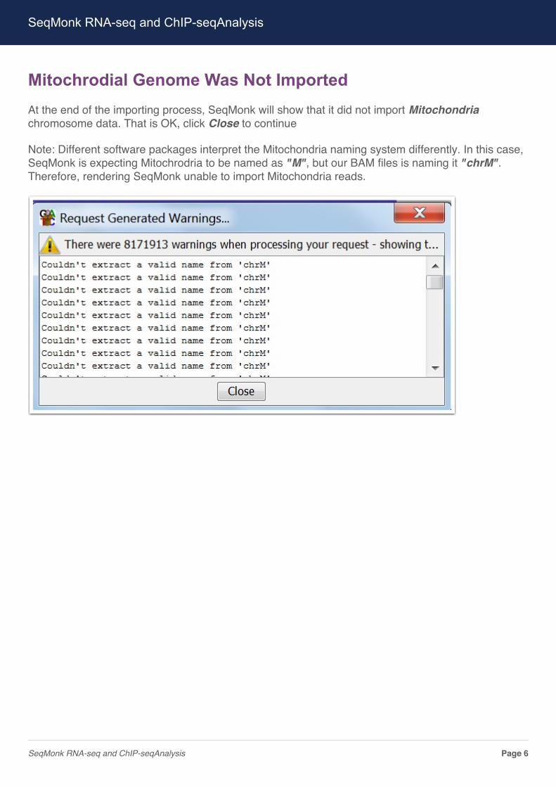
Mitochrodial Genome Was Not ImportedAt the end of the importing process, SeqMonk will show that it did not import Mitochondriachromosome data. That is OK, click Close to continue

Note: Different software packages interpret the Mitochondria naming system differently. In this case,SeqMonk is expecting Mitochrodria to be named as "M", but our BAM files is naming it "chrM".Therefore, rendering SeqMonk unable to import Mitochondria reads.



Quick Tour of Track PanelAfter suceessfully import the BAM. Examime the Track Panel to get familiar with the data layout.

Notice the referece materials:gene, mRNA and CDS

Notice the data track names as same as the BAM file namesABC_DHL2.bamABC_Ly10.bam...



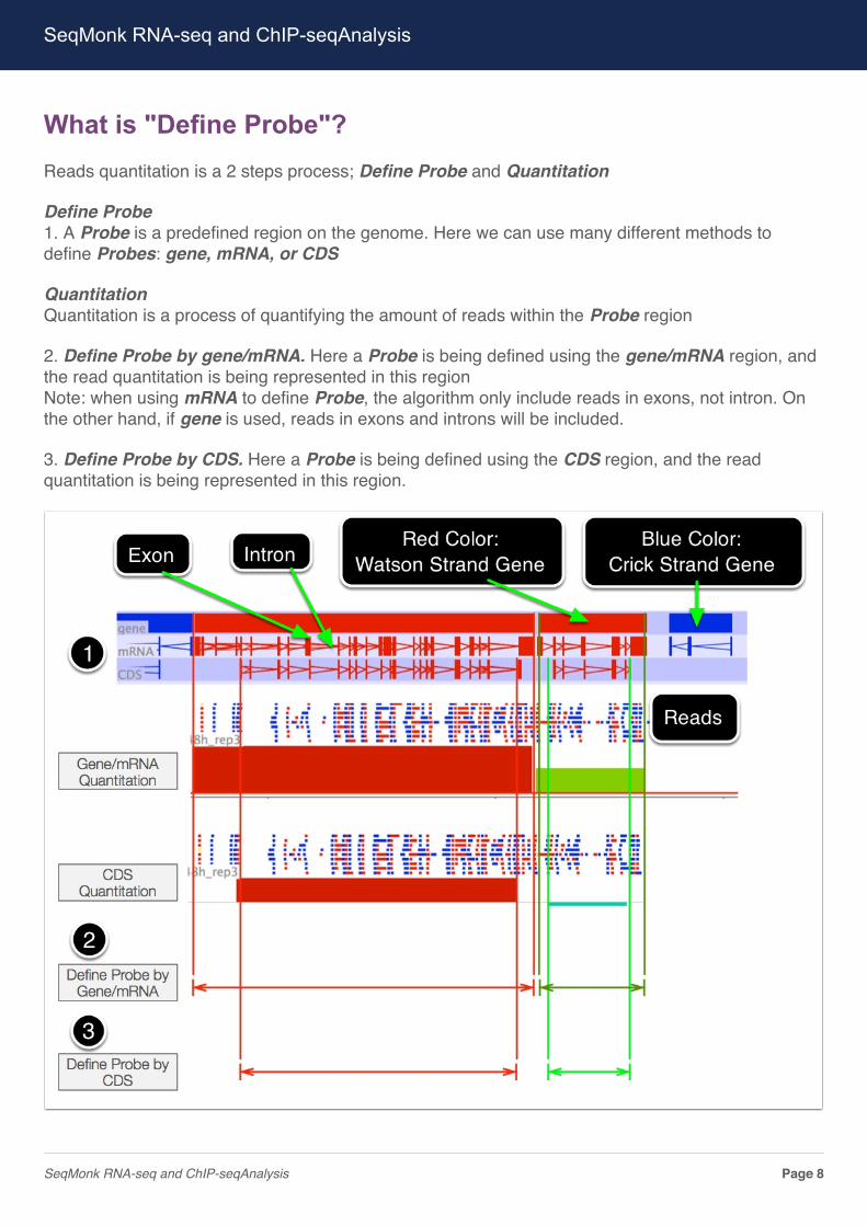
What is "Define Probe"?Reads quantitation is a 2 steps process; Define Probe and Quantitation

Define Probe1. A Probe is a predefined region on the genome. Here we can use many different methods todefine Probes: gene, mRNA, or CDS

QuantitationQuantitation is a process of quantifying the amount of reads within the Probe region

2. Define Probe by gene/mRNA. Here a Probe is being defined using the gene/mRNA region, andthe read quantitation is being represented in this regionNote: when using mRNA to define Probe, the algorithm only include reads in exons, not intron. Onthe other hand, if gene is used, reads in exons and introns will be included.

3. Define Probe by CDS. Here a Probe is being defined using the CDS region, and the readquantitation is being represented in this region.



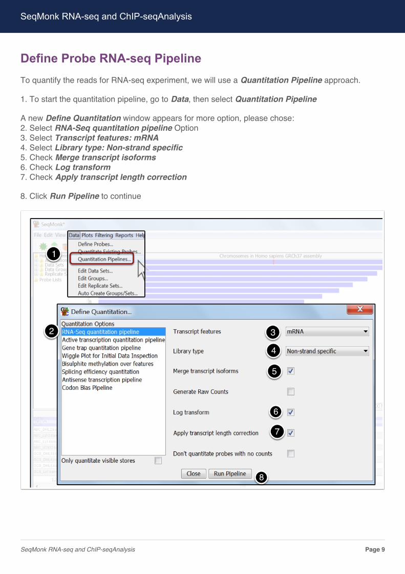
Define Probe RNA-seq PipelineTo quantify the reads for RNA-seq experiment, we will use a Quantitation Pipeline approach.

1. To start the quantitation pipeline, go to Data, then select Quantitation Pipeline

A new Define Quantitation window appears for more option, please chose:2. Select RNA-Seq quantitation pipeline Option3. Select Transcript features: mRNA4. Select Library type: Non-strand specific5. Check Merge transcript isoforms6. Check Log transform7. Check Apply transcript length correction

8. Click Run Pipeline to continue



Result of Probe DefinitionAfter read quantitation, 31,017 Probes were defined.

This is being shown on the List Panel, under the Probe Lists



QC Inspection of ReadsWe will do a visual inspection on the imported samples

1. At the Chromosome Panel, use your mouse to highlight the left most region of Chromosome 4.2. Careful examination reveals that sample ABC_Ly3.bam is particularly noisy; having readsscattered all over the region

Based on this assessment, we have decided to remove sample ABC_Ly3.bam



Remove Bad Sample1. To remove a sample, go to Data, and select Edit Data Sets ...2. On the new Edit DataSets ... window, select the bad sample ABC_Ly3.bam3. Click Delete Dataset to remove the sample from the project



Create Replicate Dataset: Step 1Next, we will group samples into 2 replicate sets: ABC and GCB

1. To group replicate set, go to Data, and chose Edit Replicate Sets...2. On the Edit Replicate Set... window, click Add New Replicate Set to add the first replicate set3. We will name the first replicate set ABC -- the new replicate set appears on the Groups box4 & 5 Repeat step 2 & 3 to add GCB replicate set

See next step on how to assign samples into each replicate set

Continues on the next page ...



Create Replicate Dataset: Step 2Assigning samples into each replicate sets

While still on the Edit Replicate Set window1. Highlight to select the ABC replicate set on the Groups box2. Highlight to select all the ABC samples (use shift key to make multiple selection)3. Click Add to assign these samples to the ABC replicate set

4. Do the same for GCB replicate set.

5. Notice the List Panel: Replicate Sets, where ABC and GCB sets were added



Add Rep Track to Track PanelWe will add the newly created Replicate Set onto the Track Panel

1. To add data track, go to View, and select Set Data Tracks ...2. In the new Select Data Track window, highlight both ABC and GCB Replicate Sets3. Click Add to add these data onto the Track Panel4. Here, it shows that the new data has been added

Note: Examine the Track Panel where the replicate sets ABC and GCB have added to the bottom ofthe tracks.



RNA-Seq QC PlotWe can perform a RNA-Seq QC Plot to determine the genomic content of our samples

1. From the Plots pull down menu, select RNA-Seq QC Plot2. Make sure only select the two duplicates: ABC and GCB. Leave the rest of the options as default3. After computation, a plot will display the percentage of various genomic content of our samples;such as Gene, Exons, rRNA, etc.

These information is important to detect contaminations



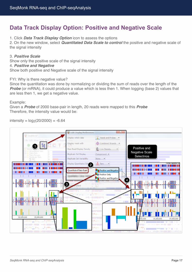
Data Track Display Option: Positive and Negative Scale1. Click Data Track Display Option icon to assess the options2. On the new window, select Quantitated Data Scale to control the positive and negative scale ofthe signal intensity

3. Positive ScaleShow only the positive scale of the signal intensity4. Positive and NegativeShow both positive and Negative scale of the signal intensity

FYI: Why is there negative value?Since the quantitation was done by normalizing or dividing the sum of reads over the length of theProbe (or mRNA), it could produce a value which is less then 1. When logging (base 2) values thatare less then 1, we get a negative value.

Example:Given a Probe of 2000 base-pair in length, 20 reads were mapped to this ProbeTherefore, the intensity value would be:

intensity = log2(20/2000) = -6.64



Data Track Display Option: Gradiant vs. Indexed Colors1. Click Data Track Display Option icon2. On the new window, select Quantitated Colour Scheme

3 Gradient ColorsWhen Gradient Colors is used, the Probe Quantitation bar change color according to the amountof reads found within the Probes.

4. Indexed ColorsWhen Indexed Colors is used, the color retain constant in the Probe Quantitation bars.



Data Track Display Option: Show Probes and Reads1. Click Data Track Display Option icon2. On the new window, select Display which data

3. Reads OnlyOnly show the reads distribution

4. Probe OnlyOnly show the Probe Quantitation bars

5. Reads and ProbeShow both the read distribution and Probe Quantitation bars together.



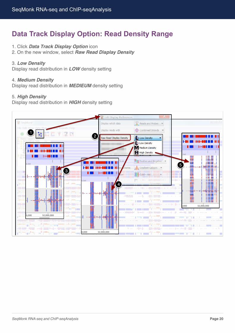
Data Track Display Option: Read Density Range1. Click Data Track Display Option icon2. On the new window, select Raw Read Display Density

3. Low DensityDisplay read distribution in LOW density setting

4. Medium DensityDisplay read distribution in MEDIEUM density setting

5. High DensityDisplay read distribution in HIGH density setting



Data Track Display Option: Combine and Separated Strands1. Click Data Track Display Option icon2. On the new window, select Display reads with

3. Separated StrandsDisplay read distribution for forward and reverse strand reads separately(Forword on top [Red], and reverse on bottom [Blue])

4. Combined StrandsDisplay read distribution by mixing the forward and reverse strand reads



Quick Access Panel: Change Annotation and Data Tracks1. Change Annotation TracksActivate to add, remove or organize the Annotation Tracks

2. Change Data TracksActivate to add, remove or organize the Data Tracks



Plot Probe Length HistogramPlot the histogram for the different Probe Length

1. Make sure to select one of the sample on the List Panel2. Go to Plots, then select Probe Length Histogram3. Most Probe (mRNA in this case), have relatively short length4. The probe length result is more apparent when set to Log scale



Plot Probe Value HistogramPlot the histogram for the overall Probe quantitation value

1. Make sure to select one of the sample on the List Panel

2. Go to Plots, then select Probe Value Histogram

3. Adjust the Division level for a more granular view of the signal

Note: The Probe Value Histogram gives us a sense of the distribution of positive vs. negative probe(mRNA in this case) quantitation. Here, we see that negative probe value is slightly higher thanpositive.



Plot Read Length HistogramPlot the histogram for the overall Read Length

1. Make sure to select one of the sample on the List Panel

2. Go to Plots, then select Read Length Histogram

3. Here, the plot shows that all reads have the same length; which is 86 nucleotide in lengthNote: the original read length is 36, recall the during the Import BAM step, we extended the readsby 50 bp. (see Page 4)



Plot BoxWhisker PlotPlot BoxWhisker Plot to assess the overall distribution of each individual sample

1. Go to Plots, then select Box Whisker Plot, follow by Visible Data Stores...2. The BoxWhisker Plot shows very even distribution among the samples, which indicates that thenormalization process was appropriate.



Plot Correlation MatrixPlot the Correlation Matrix for all data tracks

1. Go to Plots, then select Correlation Matrix...2. The Correlation Matrix shows that samples in the same group (ABC or GCB) have highercorrelation coefficient (>0.9). Although the correlation between samples from other group is not toomuch lower (~0.8). Similar to microarray experiment, we do not expect between group difference formost Probes.



Plot Scatter PlotPlot Scatter Plot to assess the relationship between the two replicate sets

1. Go to Plot, then select Scatter Plot...2. On the new window, Plot ABC vs. GCB3. Mouse over each point to see its gene symbols



Statistical Test & FDRPerform statistical test to identify genes that are significantly difference between the two replicatesets: ABC vs. GCB

1. Go to Filtering, then select Filter by Statistical Test, follow by Intensity Difference, and selectIndividual Probes ...

On the new window Intensity Difference Filter, do the following:2. On From Data Store / Group, select ABC3. On To Data Store / Group, select GCB4. On P-value must be below = 0.055. Check Apply Multiple Testing Correction6. Click Run Filter

7. On the new window Found XXX probes, give the gene list a meaningful name

8. The gene list will show up on the List Panel, under Probe Lists. In this case, we found 748statistically significant genes.



Annotate Significant Gene ListFor the newly created gene list, we will next perform annotation to give biological meaning to the list

1. Make sure to select the significant gene list

2. Go to Reports, then select Annotated Probe Report...

On the new window Annotated Probe Report Options3. On Annotate with select overlapping and gene4. Set Exclude on unannotated probes5. Click OK to proceed

Note: We did not use mRNA as annotate choice here, becuase it will return gene isoformsinformation. Instace, we have chosen to use gene which will collapse all the isoforms into a singleeasy to handle entry.



Examine the Signficant TableThe annotated table contains all the biological information about the gene list. The table can besorted using the Diff p-value column to further refine the list. Note that this column is FDR (FalseDiscovery Rate) corrected p-value. The table can be exported as text file and manipulated further inMicrosoft Excel.



Comparing Linear Statistics vs. Count StatisticsNext Generation Sequencing (NGS) produces count data. Previously, we have converted thesequencing data into linear space that allows us to use regular linear statistics, such as Student T-test, to perform statistical analysis. In the spirit of NGS inherited count statistics distribution, we willperform count statistica analysis. We need to Re-Quantitate the Probes into count space, inorder to use the count statistics methods

DESeq2edgeR

We will also perform Venn Diagram analysis using the generated gene lists.



Count Statistics QuantitationTo Re-Quantitate the Probes

1. select Quantitate Existing Probes ... from the Data pull down menu2. On the Define Quantittion ... window, select Read Count Quantitation, and leave everythingelse as blanks.3. Clink Quantitation button to begin the quantitation process.

The Quantitation process will start, and upon completion, no indicator will be presented.



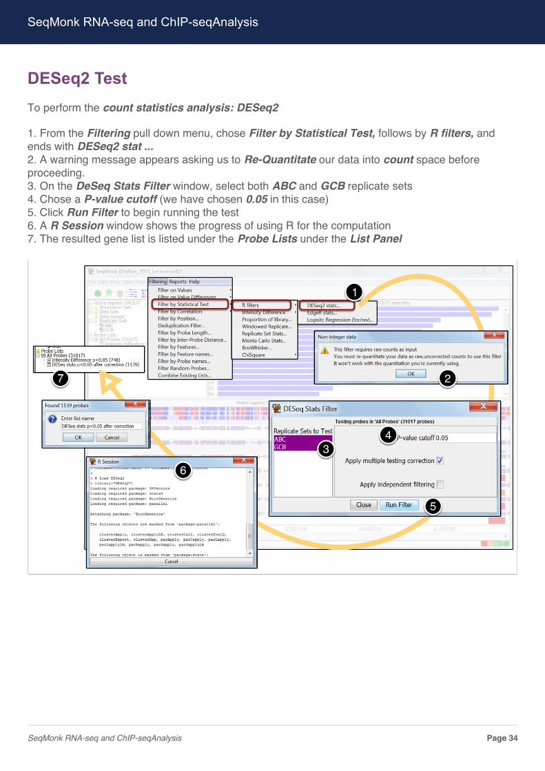
DESeq2 TestTo perform the count statistics analysis: DESeq2

1. From the Filtering pull down menu, chose Filter by Statistical Test, follows by R filters, andends with DESeq2 stat ...2. A warning message appears asking us to Re-Quantitate our data into count space beforeproceeding.3. On the DeSeq Stats Filter window, select both ABC and GCB replicate sets4. Chose a P-value cutoff (we have chosen 0.05 in this case)5. Click Run Filter to begin running the test6. A R Session window shows the progress of using R for the computation7. The resulted gene list is listed under the Probe Lists under the List Panel



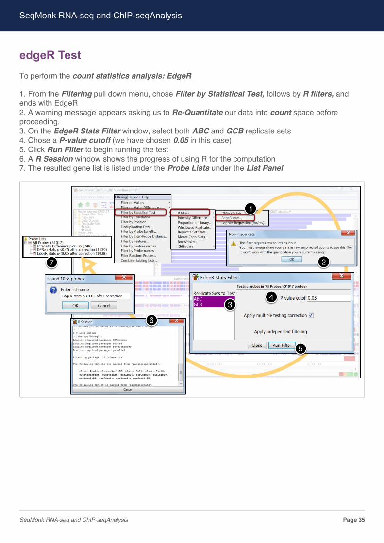
edgeR TestTo perform the count statistics analysis: EdgeR

1. From the Filtering pull down menu, chose Filter by Statistical Test, follows by R filters, andends with EdgeR2. A warning message appears asking us to Re-Quantitate our data into count space beforeproceeding.3. On the EdgeR Stats Filter window, select both ABC and GCB replicate sets4. Chose a P-value cutoff (we have chosen 0.05 in this case)5. Click Run Filter to begin running the test6. A R Session window shows the progress of using R for the computation7. The resulted gene list is listed under the Probe Lists under the List Panel



Venn DiagramNow that we have 3 significant gene list (one from linear statistics, and 2 from count statistics), wecan perform Venn Diagram analysis.

1. Select Venn Diagram ..., from the Plots pull down menu2. On the new Venn Diagram window, select Intensity Difference p<0.05 (748) and DESeq statsp<0.05 after correction (1139) for set analysis3. On the new Venn Diagram window, select EdgeR stats p<0.05 after correction (1038) andDESeq stats p<0.05 after correction (1139) for set analysis



ChIP-seq Analysis StrategyChIP-seq experiment is designed to identify the protein binding site on the genome. In this case, theauthors use ChIP-seq to locate the binding site for STAT3 protein, a Transcription Factor (TF). TFbinds to the upstream region of a Transcription Start Site (TSS), and activate the expression of thatgene. Sometimes, TF binds to other regions of the gene; such as inside and downstream of the geneboundary. To identify the potential STAT3 regulated genes, we have device a strategy to DefineProbe around the TF binding site and quantitate RNA-seq reads in the defined Probes. As shownbelow, the strategy is an attempt to capture gene expression signal surrounding the TF bindng site.We have arbituary pick 2000 base-pair up- and down-stream of the TF binding to define our probefor read quantitation purposes.



ChIP-seq Define Probe CaveatThere are some caveats using our strategy to identify STAT3 regulated genes. First, the definedProbe region might include more then one gene which can introduce complications (top figure).Second, the defined Probe region might not be large enough to capture the full extend of the gene(bottom figure).



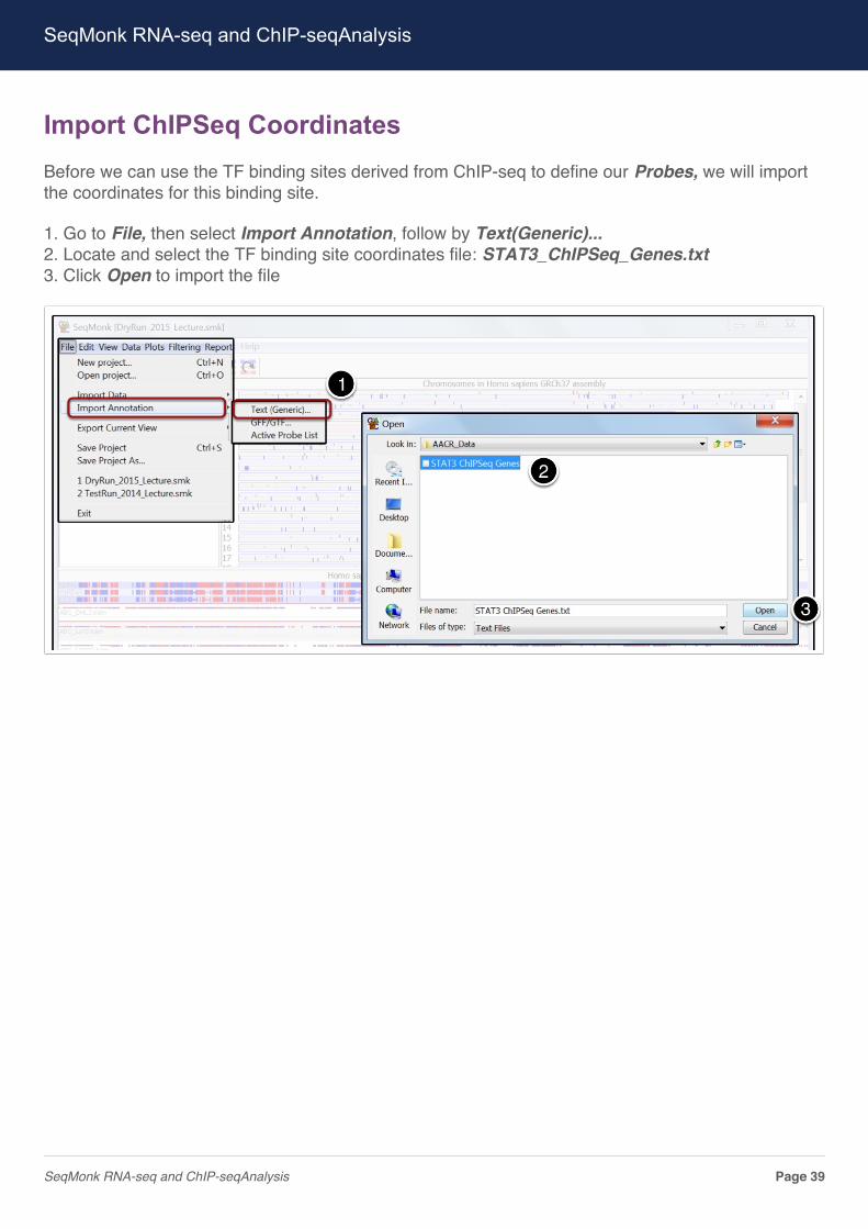
Import ChIPSeq CoordinatesBefore we can use the TF binding sites derived from ChIP-seq to define our Probes, we will importthe coordinates for this binding site.

1. Go to File, then select Import Annotation, follow by Text(Generic)...2. Locate and select the TF binding site coordinates file: STAT3_ChIPSeq_Genes.txt3. Click Open to import the file



Set ChIPSeq CoordinatesTo import a generic table, SeqMonk requires us to explicitly show it the column identifies.

1. In Start at Row, select 1 since the data starts from row number one2. In Chr Col (Chromosome Column), select 2 for the chromosome column3. In Start Col (start of genomic region), select 3 for the beginnig of the genomic region (or TFbinding site)4. In End Col (end of genomic region), select differenc 4 for the end of the genomic region.

That is all we need to provide SeqMonk to import the table.



ChIPSeq ImportedThe newly imported Annotation is listed under the List Panel, under Annotation Sets



Define Probe Using STAT3 PeaksNow that we have imported the TF binding site coordinate (see List Panel under Annotation Setsfor STAT3 ChIPSeq Genes.txt we can use them to define our Probes

1. Go to Data, then select Define Probes...

In the new Define Probes... window2. Select the Feature Probe Generator3. In Feature to design around, choose STAT3 ChIPSeq Gene.txt4. Check the Remove exact duplicate5. Check the Ignore feature strand information6. Select Over feature, and select From -2000 to +20007. Click Create Probes

Warning ........

One of the major limitation of SeqMonk is that it can only store one set of Probes. Therefore, when anew set of Probes is being defined here, the old set will be removed.

8. Click Yes to acknowledge the removal of the old set of Probes



Probe QuantitationOnce we have set up the Probe Defintion, we are now ready to quantify the reads within thoseProbes

1. Select Read Count Quantitation

In the new Define Quantitation window2. In Count reads in strand, select All Reads3. Check the Correct for total read cont:4. In Correct to what? chose Largest DataStore5. Check the Count total only within probes6. Check the Correct for probe length7. Check the Log Transform Count8. Click Quantitate to proceed



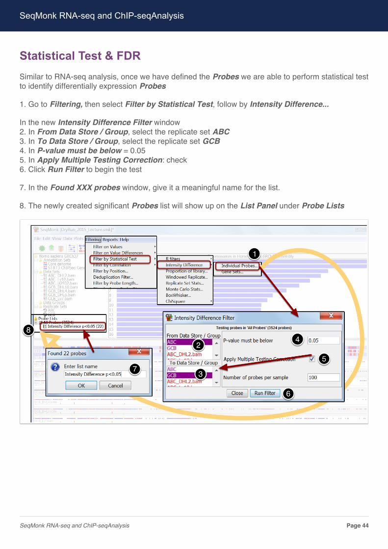
Statistical Test & FDRSimilar to RNA-seq analysis, once we have defined the Probes we are able to perform statistical testto identify differentially expression Probes

1. Go to Filtering, then select Filter by Statistical Test, follow by Intensity Difference...

In the new Intensity Difference Filter window2. In From Data Store / Group, select the replicate set ABC3. In To Data Store / Group, select the replicate set GCB4. In P-value must be below = 0.055. In Apply Multiple Testing Correction: check6. Click Run Filter to begin the test

7. In the Found XXX probes window, give it a meaningful name for the list.

8. The newly created significant Probes list will show up on the List Panel under Probe Lists



Annotate STAT3 Regulated GenesThe newly created potential STAT3 regulated genes is annotated to give biological meaning to thelist

1. Go to Report, then select Annotated Probes Report...

In the new Annotated Probe Report Options window2. In Annotate with, select closest and gene3. In Annotation distance cutoff type 10,000 bp4. Select Exclude, unannotated probes5. Select Include, data for currently visible stores6. Click OK to proceed



Potential STAT3 Regulated GenesThe annotated table contains all the biological information about the gene list. The table can besorted using the Diff p-value column to further refine the list. Note that this column is FDR (FalseDiscovery Rate) corrected p-value. The table can be exported as text file and manipulated further inMicrosoft Excel.Note: * (Asterisk) represent genes reported in the paper we found in our analysis



Ingenuity Pathway AnalysisThe instructor for this section (Dr. Edwards) will expect that the workshop participants will havewatched the video, “Understanding Bioinformatics: Finding the Biology in a List of Genes” beforeattending the laboratory. This ~20 min. video provides background information on the types ofbiological information we look for in a list of genes. Dr. Edwards has also provided video tutorials oflast year’s AACR workshop for those that wanted to get a head start on the lesson plan. Therequired video and additional instructional material can be found at Dr. Edwards’ YouTube channelat the following links:

Michael Edwards YouTube channel

• (https://www.youtube.com/channel/UCUAyxGdB-3uNJkee2qvHKCg)

Understanding Bioinformatics Video (required)

• https://www.youtube.com/watch?v=uOAgGrD4lbM

2014 AACR Workshop Genomics and Bioinformatics (optional)

• https://www.youtube.com/playlist?list=PLCQx4mwID7jtniWdoLkKbKzzwNPVZXETX

Additional tutorials using Ingenuity Pathway Analysis software

• https://www.youtube.com/playlist?list=PLCQx4mwID7js2su2SNBNF_N9o063eInmn

Participants for this workshop are encouraged to bring in their own gene lists to analyze atthe end of this session. Please make sure all gene lists include an established gene identifier(gene symbol, refseq #, Affymetrix probeset ID, etc…), fold change and p-value information.



https://www.youtube.com/channel/UCUAyxGdB-3uNJkee2qvHKCg

https://www.youtube.com/watch?v=uOAgGrD4lbM

https://www.youtube.com/playlist?list=PLCQx4mwID7jtniWdoLkKbKzzwNPVZXETX

https://www.youtube.com/playlist?list=PLCQx4mwID7js2su2SNBNF_N9o063eInmn

SeqMonk RNA-seq and ChIP-seqAnalysis

Documents

Transcript of SeqMonk RNA-seq and ChIP-seqAnalysis