arX

iv:0

910.

1122

v1 [

mat

h.ST

] 6

Oct

200

9

Invited Review Article: A Selective Overview of Variable

Selection in High Dimensional Feature Space

Jianqing Fan and Jinchi Lv ∗

Princeton University and University of Southern California

September 1, 2009

Abstract

High dimensional statistical problems arise from diverse fields of scientific research

and technological development. Variable selection plays a pivotal role in contemporary

statistical learning and scientific discoveries. The traditional idea of best subset selection

methods, which can be regarded as a specific form of penalized likelihood, is computa-

tionally too expensive for many modern statistical applications. Other forms of penalized

likelihood methods have been successfully developed over the last decade to cope with

high dimensionality. They have been widely applied for simultaneously selecting im-

portant variables and estimating their effects in high dimensional statistical inference.

In this article, we present a brief account of the recent developments of theory, meth-

ods, and implementations for high dimensional variable selection. What limits of the

dimensionality such methods can handle, what the role of penalty functions is, and what

the statistical properties are rapidly drive the advances of the field. The properties of

non-concave penalized likelihood and its roles in high dimensional statistical modeling

are emphasized. We also review some recent advances in ultra-high dimensional variable

selection, with emphasis on independence screening and two-scale methods.

Short title: Variable Selection in High Dimensional Feature Space

AMS 2000 subject classifications: Primary 62J99; secondary 62F12, 68Q32

Key words and phrases: Variable selection, model selection, high dimensionality, penal-

ized least squares, penalized likelihood, folded-concave penalty, oracle property, dimension-

ality reduction, LASSO, SCAD, sure screening, sure independence screening

∗Jianqing Fan is Frederick L. Moore ’18 Professor of Finance, Department of Operations Research and

Financial Engineering, Princeton University, Princeton, NJ 08544, USA (e-mail: jqfan@princeton.edu).

Jinchi Lv is Assistant Professor of Statistics, Information and Operations Management Department, Mar-

shall School of Business, University of Southern California, Los Angeles, CA 90089, USA (e-mail: jin-

chilv@marshall.usc.edu). Fan’s research was partially supported by NSF Grants DMS-0704337 and DMS-

0714554 and NIH Grant R01-GM072611. Lv’s research was partially supported by NSF Grant DMS-0806030

and 2008 Zumberge Individual Award from USC’s James H. Zumberge Faculty Research and Innovation Fund.

We sincerely thank the Co-Editor, Professor Peter Hall, for his kind invitation to write this article. We are

also very grateful to the helpful comments of the Co-Editor, Associate Editor and referees that substantially

improved the presentation of the paper.

1

1 Introduction

High dimensional data analysis has become increasingly frequent and important in diverse

fields of sciences, engineering, and humanities, ranging from genomics and health sciences

to economics, finance and machine learning. It characterizes many contemporary problems

in statistics (Hastie, Tibshirani and Friedman (2009)). For example, in disease classification

using microarray or proteomics data, tens of thousands of expressions of molecules or ions

are potential predictors; in genowide association studies between genotypes and phenotypes,

hundreds of thousands of SNPs are potential covariates for phenotypes such as cholesterol

levels or heights. When interactions are considered, the dimensionality grows quickly. For ex-

ample, in portfolio allocation among two thousand stocks, it involves already over two million

parameters in the covariance matrix; interactions of molecules in the above examples result in

ultra-high dimensionality. To be more precise, throughout the paper ultra-high dimensional-

ity refers to the case where the dimensionality grows at a non-polynomial rate as the sample

size increases, and high dimensionality refers to the general case of growing dimensionality.

Other examples of high dimensional data include high-resolution images, high-frequency fi-

nancial data, e-commerce data, warehouse data, functional, and longitudinal data, among

others. Donoho (2000) convincingly demonstrates the need for developments in high dimen-

sional data analysis, and presents the curses and blessings of dimensionality. Fan and Li

(2006) give a comprehensive overview of statistical challenges with high dimensionality in a

broad range of topics, and in particular, demonstrate that for a host of statistical problems,

the model parameters can be estimated as well as if the best model is known in advance,

as long as the dimensionality is not excessively high. The challenges that are not present in

smaller scale studies have been reshaping statistical thinking, methodological development,

and theoretical studies.

Statistical accuracy, model interpretability, and computational complexity are three im-

portant pillars of any statistical procedures. In conventional studies, the number of observa-

tions n is much larger than the number of variables or parameters p. In such cases, none of

the three aspects needs to be sacrificed for the efficiency of others. The traditional methods,

however, face significant challenges when the dimensionality p is comparable to or larger

than the sample size n. These challenges include how to design statistical procedures that

are more efficient in inference; how to derive the asymptotic or nonasymptotic theory; how

to make the estimated models interpretable; and how to make the statistical procedures

computationally efficient and robust.

A notorious difficulty of high dimensional model selection comes from the collinearity

among the predictors. The collinearity can easily be spurious in high dimensional geometry

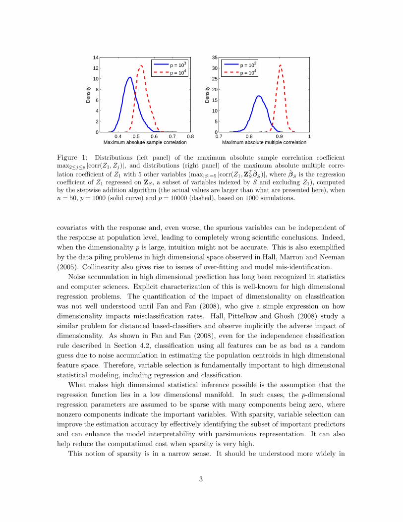
(Fan and Lv (2008)), which can make us select a wrong model. Figure 1 shows the maximum

sample correlation and multiple correlation with a given predictor despite that predictors are

generated from independent Gaussian random variables. As a result, any variable can be

well-approximated even by a couple of spurious variables, and can even be replaced by them

when the dimensionality is much higher than the sample size. If that variable is a signature

predictor and is replaced by spurious variables, we choose wrong variables to associate the

2

0.4 0.5 0.6 0.7 0.80

2

4

6

8

10

12

14

Maximum absolute sample correlation

Den

sity

0.7 0.8 0.9 10

5

10

15

20

25

30

35

Maximum absolute multiple correlation

Den

sity

p = 103

p = 104p = 103

p = 104

Figure 1: Distributions (left panel) of the maximum absolute sample correlation coefficientmax2≤j≤p |corr(Z1, Zj)|, and distributions (right panel) of the maximum absolute multiple corre-

lation coefficient of Z1 with 5 other variables (max|S|=5 |corr(Z1,ZTS βS)|, where βS is the regression

coefficient of Z1 regressed on ZS , a subset of variables indexed by S and excluding Z1), computedby the stepwise addition algorithm (the actual values are larger than what are presented here), whenn = 50, p = 1000 (solid curve) and p = 10000 (dashed), based on 1000 simulations.

covariates with the response and, even worse, the spurious variables can be independent of

the response at population level, leading to completely wrong scientific conclusions. Indeed,

when the dimensionality p is large, intuition might not be accurate. This is also exemplified

by the data piling problems in high dimensional space observed in Hall, Marron and Neeman

(2005). Collinearity also gives rise to issues of over-fitting and model mis-identification.

Noise accumulation in high dimensional prediction has long been recognized in statistics

and computer sciences. Explicit characterization of this is well-known for high dimensional

regression problems. The quantification of the impact of dimensionality on classification

was not well understood until Fan and Fan (2008), who give a simple expression on how

dimensionality impacts misclassification rates. Hall, Pittelkow and Ghosh (2008) study a

similar problem for distanced based-classifiers and observe implicitly the adverse impact of

dimensionality. As shown in Fan and Fan (2008), even for the independence classification

rule described in Section 4.2, classification using all features can be as bad as a random

guess due to noise accumulation in estimating the population centroids in high dimensional

feature space. Therefore, variable selection is fundamentally important to high dimensional

statistical modeling, including regression and classification.

What makes high dimensional statistical inference possible is the assumption that the

regression function lies in a low dimensional manifold. In such cases, the p-dimensional

regression parameters are assumed to be sparse with many components being zero, where

nonzero components indicate the important variables. With sparsity, variable selection can

improve the estimation accuracy by effectively identifying the subset of important predictors

and can enhance the model interpretability with parsimonious representation. It can also

help reduce the computational cost when sparsity is very high.

This notion of sparsity is in a narrow sense. It should be understood more widely in

3

transformed or enlarged feature spaces. For instance, some prior knowledge may lead us to

apply some grouping or transformation of the input variables (see, e.g., Fan and Lv (2008)).

Some transformation of the variables may be appropriate if a significant portion of the

pairwise correlations are high. In some cases, we may want to enlarge the feature space by

adding interactions and higher order terms to reduce the bias of the model. Sparsity can also

be viewed in the context of dimensionality reduction by introducing a sparse representation,

i.e., by reducing the number of effective parameters in estimation. Examples include the

use of a factor model for high dimensional covariance matrix estimation in Fan, Fan and Lv

(2008).

Sparsity arises in many scientific endeavors. In genomic studies, it is generally believed

that only a fraction of molecules are related to biological outcomes. For example, in disease

classification, it is commonly believed that only tens of genes are responsible for a disease.

Selecting tens of genes helps not only statisticians in constructing a more reliable classifi-

cation rule, but also biologists to understand molecular mechanisms. In contrast, popular

but naive methods used in microarray data analysis (Dudoit, Shaffer and Boldrick (2003);

Storey and Tibshirani (2003); Fan and Ren (2006); Efron (2007)) rely on two-sample tests

to pick important genes, which is truly a marginal correlation ranking (Fan and Lv (2008))

and can miss important signature genes (Fan, Samworth and Wu (2009)). The main goals

of high dimensional regression and classification, according to Bickel (2008), are

• to construct as effective a method as possible to predict future observations;

• to gain insight into the relationship between features and response for scientific pur-

poses, as well as, hopefully, to construct an improved prediction method.

The former appears in problems such as text and document classification or portfolio opti-

mization, whereas the latter appears naturally in many genomic studies and other scientific

endeavors.

As pointed out in Fan and Li (2006), it is helpful to differentiate two types of statistical

endeavors in high dimensional statistical learning: accuracy of estimated model parameters

and accuracy of the expected loss of the estimated model. The latter property is called

persistence in Greenshtein and Ritov (2004) and Greenshtein (2006), and arises frequently

in machine learning problems such as document classification and computer vision. The

former appears in many other contexts where we want to identify the significant predictors

and characterize the precise contribution of each to the response variable. Examples include

health studies, where the relative importance of identified risk factors needs to be assessed for

prognosis. Many of the existing results in the literature have been concerned with the study

of consistency of high dimensional variable selection methods, rather than characterizing

the asymptotic distributions of the estimated model parameters. However, consistency and

persistence results are inadequate for understanding uncertainty in parameter estimation.

High dimensional variable selection encompasses a majority of frontiers where statistics

advances rapidly today. There has been an evolving literature in the last decade devoted to

understanding the performance of various variable selection techniques. The main theoretical

4

questions include determining the limits of the dimensionality that such methods can handle

and how to characterize the optimality of variable selection procedures. The answers to the

first question for many existing methods were largely unknown until recently. To a large

extent, the second question still remains open for many procedures. In the Gaussian linear

regression model, the case of orthonormal design reduces to the problem of Gaussian mean

estimation, as do the wavelet settings where the design matrices are orthogonal. In such

cases, the risks of various shrinkage estimators and their optimality have been extensively

studied. See, e.g., Donoho and Johnstone (1994) and Antoniadis and Fan (2001).

In this article we address the issues of variable selection for high dimensional statisti-

cal modeling in the unified framework of penalized likelihood estimation. It has been widely

used in statistical inferences and machine learning, and is basically a moderate scale learning

technique. We also give an overview on the techniques for ultrahigh dimensional screening.

Combined iteratively with large scale screening, it can handle problems of ultra-high dimen-

sionality (Fan, Samworth and Wu (2009)). This will be reviewed as well.

The rest of the article is organized as follows. In Section 2, we discuss the connections

of penalized likelihood to classical model selection methods. Section 3 details the methods

and implementation of penalized likelihood estimation. We review some recent advances in

ultra-high dimensional variable selection in Section 4. In Section 5, we survey the sampling

properties of penalized least squares. Section 6 presents the classical oracle property of

penalized least squares and penalized likelihood methods in ultra-high dimensional space.

We conclude the article with some additional remarks in Section 7.

2 Classical model selection

Suppose that the available data are (xTi , yi)

ni=1, where yi is the i-th observation of the response

variable and xi is its associated p-dimensional covariates vector. They are usually assumed

to be a random sample from the population (XT , Y ), where the conditional mean of Y given

X depends on the linear predictor βTX with β = (β1, · · · , βp)T . In sparse modeling, it is

frequently assumed that most regression coefficients βj are zero. Variable selection aims to

identify all important variables whose regression coefficients do not vanish and to provide

effective estimates of those coefficients.

More generally, assume that the data are generated from the true density function fθ0

with parameter vector θ0 = (θ1, · · · , θd)T . Often, we are uncertain about the true density,

but more certain about a larger family of models fθ1in which θ0 is a (nonvanishing) subvector

of the p-dimensional parameter vector θ1. The problems of how to estimate the dimension

of the model and compare models of different dimensions naturally arise in many statistical

applications, including time series modeling. These are referred to as model selection in the

literature.

Akaike (1973, 1974) proposes to choose a model that minimizes the Kullback-Leibler (KL)

divergence of the fitted model from the true model. Akaike (1973) considers the maximum

likelihood estimator (MLE) θ = (θ1, · · · , θp)T of the parameter vector θ and shows that, up

5

to an additive constant, the estimated KL divergence can be asymptotically expanded as

−ℓn(θ) + λdim(θ) = −ℓn(θ) + λ

p∑

j=1

I(θj 6= 0),

where ℓn(θ) is the log-likelihood function, dim(θ) denotes the dimension of the model, and

λ = 1. This leads to the AIC. Schwartz (1978) takes a Bayesian approach with prior dis-

tributions that have nonzero prior probabilities on some lower dimensional subspaces and

proposes the BIC with λ = (log n)/2 for model selection. Recently, Lv and Liu (2008) gave a

KL divergence interpretation of Bayesian model selection and derive generalizations of AIC

and BIC when the model may be misspecified.

The work of AIC and BIC suggests a unified approach to model selection: choose a

parameter vector θ that maximizes the penalized likelihood

ℓn(θ) − λ‖θ‖0, (1)

where the L0-norm of θ counts the number of non-vanishing components in θ and λ ≥ 0

is a regularization parameter. Given ‖θ‖0 = m, the solution to (1) is the subset with the

largest maximum likelihood among all subsets of size m. The model size m is then chosen

to maximize (1) among p best subsets of sizes m (1 ≤ m ≤ p). Clearly, the computation of

the penalized L0 problem is a combinational problem with NP-complexity.

When the normal likelihood is used, (1) becomes penalized least squares. Many tradi-

tional methods can be regarded as penalized likelihood methods with different choices of

λ. Let RSSd be the residual sum of squares of the best subset with d variables. Then

Cp = RSSd/s2 + 2d − n in Mallows (1973) corresponds to λ = 1, where s2 is the mean

squared error of the full model. The adjusted R2 given by

R2adj = 1 − n− 1

n− d

RSSd

SST

also amounts to a penalized-L0 problem, where SST is the total sum of squares. Clearly

maximizing R2adj is equivalent to minimizing log(RSSd/(n− d)). By RSSd/n ≈ σ2 (the error

variance), we have

n logRSSd

n− d≈ RSSd/σ

2 + d+ n(log σ2 − 1).

This shows that the adjusted R2 method is approximately equivalent to PMLE with λ = 1/2.

Other examples include the generalized cross-validation (GCV) given by RSSd/(1 − d/n)2,

cross-validation (CV), and RIC in Foster and George (1994). See Bickel and Li (2006) for

more discussions of regularization in statistics.

3 Penalized likelihood

As demonstrated above, L0 regularization arises naturally in many classical model selection

methods. It gives a nice interpretation of best subset selection and admits nice sampling

6

properties (Barron, Birge and Massart (1999)). However, the computation is infeasible in

high dimensional statistical endeavors. Other penalty functions should be used. This results

in a generalized form

n−1ℓn(β) −p∑

j=1

pλ(|βj |), (2)

where ℓn(β) is the log-likelihood function and pλ(·) is a penalty function indexed by the

regularization parameter λ ≥ 0. By maximizing the penalized likelihood (2), we hope to

simultaneously select variables and estimate their associated regression coefficients. In other

words, those variables whose regression coefficients are estimated as zero are automatically

deleted.

A natural generalization of penalized L0-regression is penalized Lq-regression, called

bridge regression in Frank and Friedman (1993), in which pλ(|θ|) = λ|θ|q for 0 < q ≤ 2.

This bridges the best subset section (penalized L0) and ridge regression (penalized L2), in-

cluding the L1-penalty as a specific case. The non-negative garrote is introduced in Breiman

(1995) for shrinkage estimation and variable selection. Penalized L1-regression is called the

LASSO by Tibshirani (1996) in the ordinary regression setting, and is now collectively re-

ferred to as penalized L1-likelihood. Clearly, penalized L0-regression possesses the variable

selection feature, whereas penalized L2-regression does not. What kind of penalty functions

are good for model selection?

Fan and Li (2001) advocate penalty functions that give estimators with three properties:

1) Sparsity : The resulting estimator automatically sets small estimated coefficients to

zero to accomplish variable selection and reduce model complexity.

2) Unbiasedness: The resulting estimator is nearly unbiased, especially when the true

coefficient βj is large, to reduce model bias.

3) Continuity : The resulting estimator is continuous in the data to reduce instability in

model prediction (Breiman (1996)).

They require the penalty function pλ(|θ|) to be nondecreasing in |θ|, and provide insights

into these properties. We first consider the penalized least squares in a canonical form.

3.1 Canonical regression model

Consider the linear regression model

y = Xβ + ε, (3)

where X = (x1, · · · ,xn)T , y = (y1, · · · , yn)T , and ε is an n-dimensional noise vector. If

ε ∼ N(0, σ2In), then the penalized likelihood (2) is equivalent, up to an affine transformation

of the log-likelihood, to the penalized least squares (PLS) problem

minβ∈Rp

1

2n‖y− Xβ‖2 +

p∑

j=1

pλ(|βj |)

, (4)

7

where ‖ · ‖ denotes the L2-norm. Of course, the penalized least squares continues to be

applicable even when the noise does not follow a normal distribution.

For the canonical linear model in which the design matrix multiplied by n−1/2 is or-

thonormal (i.e., XTX = nIp), (4) reduces to the minimization of

1

2n‖y − Xβ‖2 + ‖β − β‖2 +

p∑

j=1

pλ(|βj |), (5)

where β = n−1XTy is the ordinary least squares estimate. Minimizing (5) becomes a

componentwise regression problem. This leads to considering the univariate PLS problem

θ(z) = arg minθ∈R

{1

2(z − θ)2 + pλ(|θ|)

}. (6)

Antoniadis and Fan (2001) show that the PLS estimator θ(z) possesses the properties:

1) sparsity if mint≥0{t+ p′λ(t)} > 0;

2) approximate unbiasedness if p′λ(t) = 0 for large t;

3) continuity if and only if arg mint≥0{t+ p′λ(t)} = 0,

where pλ(t) is nondecreasing and continuously differentiable on [0,∞), the function −t−p′λ(t)

is strictly unimodal on (0,∞), and p′λ(t) means p′λ(0+) when t = 0 for notational simplicity.

In general for the penalty function, the singularity at the origin (i.e., p′λ(0+) > 0) is needed for

generating sparsity in variable selection and the concavity is needed to reduce the estimation

bias.

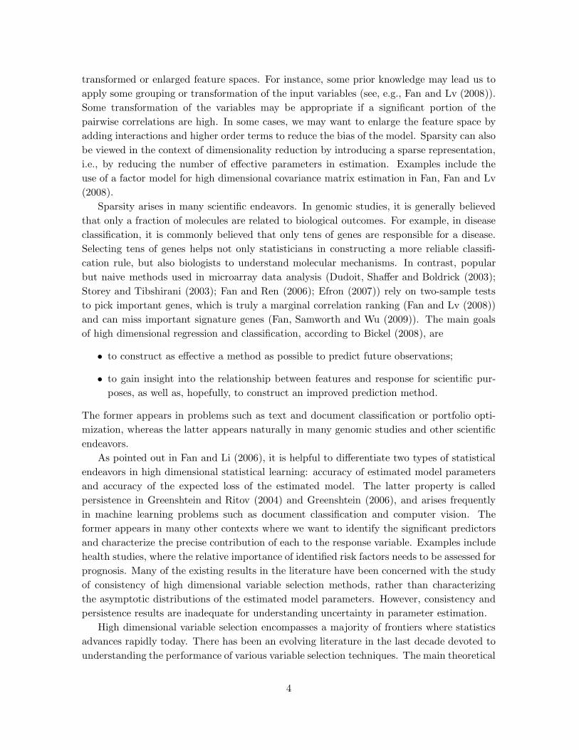
3.2 Penalty function

It is known that the convex Lq penalty with q > 1 does not satisfy the sparsity condition,

whereas the convex L1 penalty does not satisfy the unbiasedness condition, and the concave

Lq penalty with 0 ≤ q < 1 does not satisfy the continuity condition. In other words, none

of the Lq penalties satisfies all three conditions simultaneously. For this reason, Fan (1997)

and Fan and Li (2001) introduce the smoothly clipped absolute deviation (SCAD), whose

derivative is given by

p′λ(t) = λ

{I (t ≤ λ) +

(aλ− t)+(a− 1)λ

I (t > λ)

}for some a > 2, (7)

where pλ(0) = 0 and, often, a = 3.7 is used (suggested by a Bayesian argument). It satisfies

the aforementioned three properties. A penalty of similar spirit is the minimax concave

penalty (MCP) in Zhang (2009), whose derivative is given by

p′λ(t) = (aλ− t)+ /a. (8)

8

−10 −5 0 5 100

2

4

6

8

10

θ

p λ(|θ|

)

SCADMCPHardSoft

0 2 4 6 80

0.5

1

1.5

2

2.5

3

3.5

4

θ

p λ’(|θ|

)

SCADMCPHardSoft

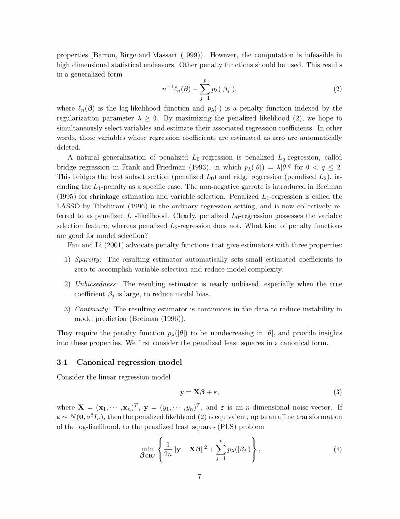
Figure 2: Some commonly used penalty functions (left panel) and their derivatives (right panel).They correspond to the risk functions shown in the right panel of Figure 3. More precisely, λ = 2 forhard thresholding penalty, λ = 1.04 for L1-penalty, λ = 1.02 for SCAD with a = 3.7, and λ = 1.49for MCP with a = 2.

Clearly SCAD takes off at the origin as the L1 penalty and then gradually levels off, and

MCP translates the flat part of the derivative of SCAD to the origin. When

pλ(t) = λ2 − (λ− t)2+, (9)

Antoniadis (1996) shows that the solution is the hard-thresholding estimator θH(z) = zI(|z| >λ). A family of concave penalties that bridge the L0 and L1 penalties is studied by Lv and Fan

(2009) for model selection and sparse recovery. A linear combination of L1 and L2 penalties

is called an elastic net by Zou and Hastie (2005), which encourages some grouping effects.

Figure 2 depicts some of those commonly used penalty functions.

We now look at the PLS estimator θ(z) in (6) for a few penalties. Each increasing penalty

function gives a shrinkage rule: |θ(z)| ≤ |z| and θ(z) = sgn(z)|θ(z)| (Antoniadis and Fan

(2001)). The entropy penalty (L0 penalty) and the hard thresholding penalty yield the

hard thresholding rule (Donoho and Johnstone (1994)), while the L1 penalty gives the soft

thresholding rule (Bickel (1983); Donoho and Johnstone (1994)). The SCAD and MCP give

rise to analytical solutions to (6), each of which is a linear spline in z (Fan (1997)).

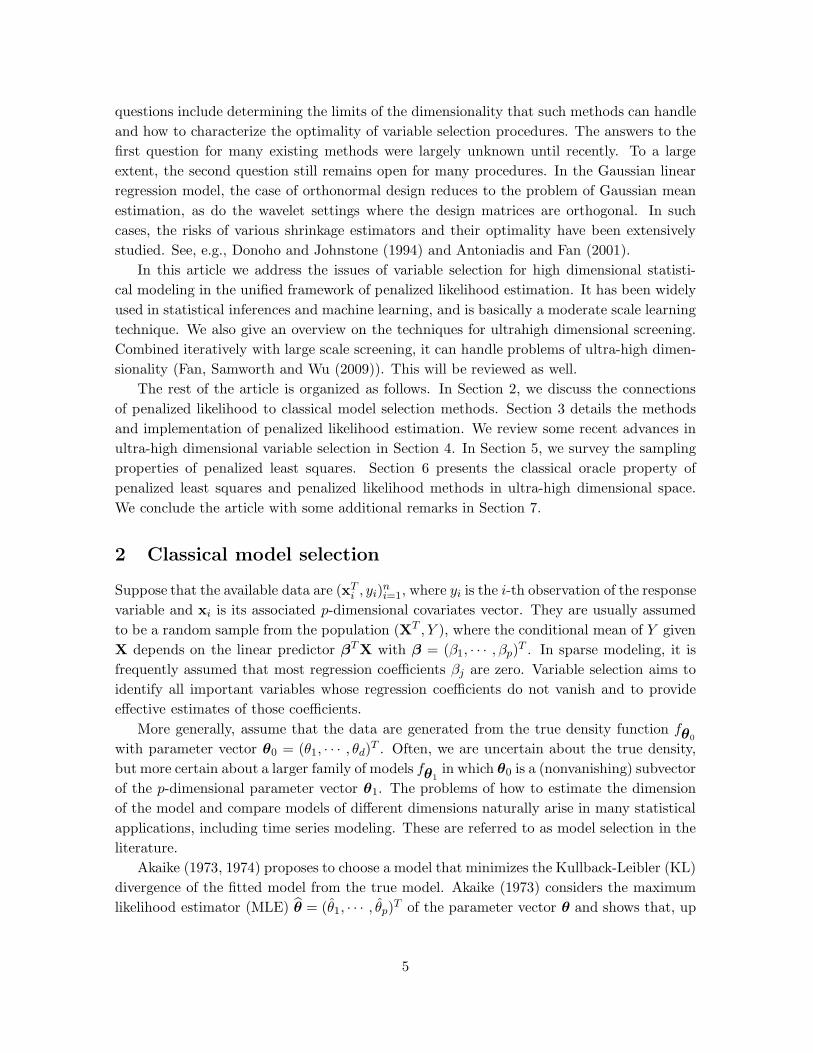
How do those thresholded-shrinkage estimators perform? To compare them, we compute

their risks in the fundamental model in which Z ∼ N(θ, 1). Let R(θ) = E(θ(Z) − θ)2.

Figure 3 shows the risk functions R(θ) for some commonly used penalty functions. To make

them comparable, we chose λ = 1 and 2 for the hard thresholding penalty, and for other

penalty functions the values of λ were chosen to make their risks at θ = 3 the same. Clearly

the penalized likelihood estimators improve the ordinary least squares estimator Z in the

region where θ is near zero, and have the same risk as the ordinary least squares estimator

when θ is far away from zero (e.g., 4 standard deviations away), except the LASSO estimator.

When θ is large, the LASSO estimator has a bias approximately of size λ, and this causes

higher risk as shown in Figure 3. When λhard = 2, the LASSO estimator has higher risk

than the SCAD estimator, except in a small region. The bias of the LASSO estimator makes

9

−10 −5 0 5 10

0.7

0.8

0.9

1

1.1

1.2

1.3

1.4

θ

Ris

k

λhard

= 1

SCADMCPHardSoft

−10 −5 0 5 100

0.5

1

1.5

2

2.5

3

θ

Ris

k

λhard

= 2

SCADMCPHardSoft

Figure 3: The risk functions for penalized least squares under the Gaussian model for the hard-thresholding penalty, L1-penalty, SCAD (a = 3.7), and MCP (a = 2). The left panel corresponds toλ = 1 and the right panel corresponds to λ = 2 for the hard-thresholding estimator, and the rest ofparameters are chosen so that their risks are the same at the point θ = 3.

LASSO prefer a smaller λ. For λhard = 1, the advantage of the LASSO estimator around

zero is more pronounced. As a result in model selection, when λ is automatically selected

by a data-driven rule to compensate the bias problem, the LASSO estimator has to choose a

smaller λ in order to have a desired mean squared error. Yet, a smaller value of λ results in

a complex model. This explains why the LASSO estimator tends to have many false positive

variables in the selected model.

3.3 Computation and implementation

It is challenging to solve the penalized likelihood problem (2) when the penalty function pλ

is nonconvex. Nevertheless, Fan and Lv (2009) are able to give the conditions under which

the penalized likelihood estimator exists and is unique; see also Kim and Kwon (2009) for

the results of penalized least squares with SCAD penalty. When the L1-penalty is used,

the objective function (2) is concave and hence convex optimization algorithms can be ap-

plied. We show in this section that the penalized likelihood (2) can be solved by a sequence

of reweighted penalized L1-regression problems via local linear approximation (Zou and Li

(2008)).

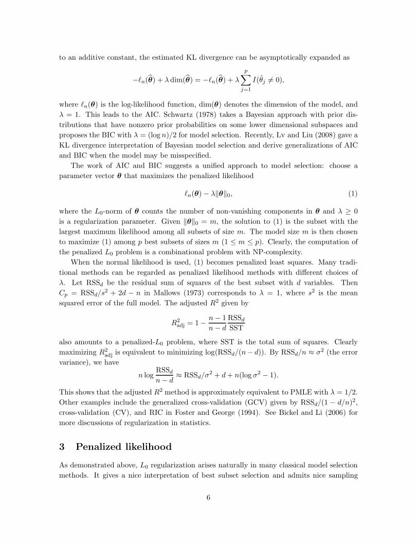
In the absence of other available algorithms at that time, Fan and Li (2001) propose a

unified and effective local quadratic approximation (LQA) algorithm for optimizing noncon-

cave penalized likelihood. Their idea is to locally approximate the objective function by a

quadratic function. Specifically, for a given initial value β∗ = (β∗1 , · · · , β∗p)T , the penalty

function pλ can be locally approximated by a quadratic function as

pλ(|βj |) ≈ pλ(|β∗j |) +1

2

p′λ(|β∗j |)|β∗j |

[β2j − (β∗j )2] for βj ≈ β∗j . (10)

With this and a LQA to the log-likelihood, the penalized likelihood (2) becomes a least

squares problem that admits a closed-form solution. To avoid numerical instability, it sets

10

−10 −5 0 5 100

5

10

15

20

25

θ

Pen

alty

Figure 4: The local linear (dashed) and local quadratic (dotted) approximations to the SCADfunction (solid) with λ = 2 and a = 3.7 at a given point |θ| = 4.

the estimated coefficient βj = 0 if β∗j is very close to 0, which amounts to deleting the j-th

covariate from the final model. Clearly the value 0 is an absorbing state of LQA in the sense

that once a coefficient is set to zero, it remains zero in subsequent iterations.

The convergence property of the LQA was studied in Hunter and Li (2005), who show

that LQA plays the same role as the E-step in the EM algorithm in Dempster, Laird and Rubin

(1977). Therefore LQA has similar behavior to EM. Although the EM requires a full itera-

tion for maximization after each E-step, the LQA updates the quadratic approximation at

each step during the course of iteration, which speeds up the convergence of the algorithm.

The convergence rate of LQA is quadratic, which is the same as that of the modified EM

algorithm in Lange (1995).

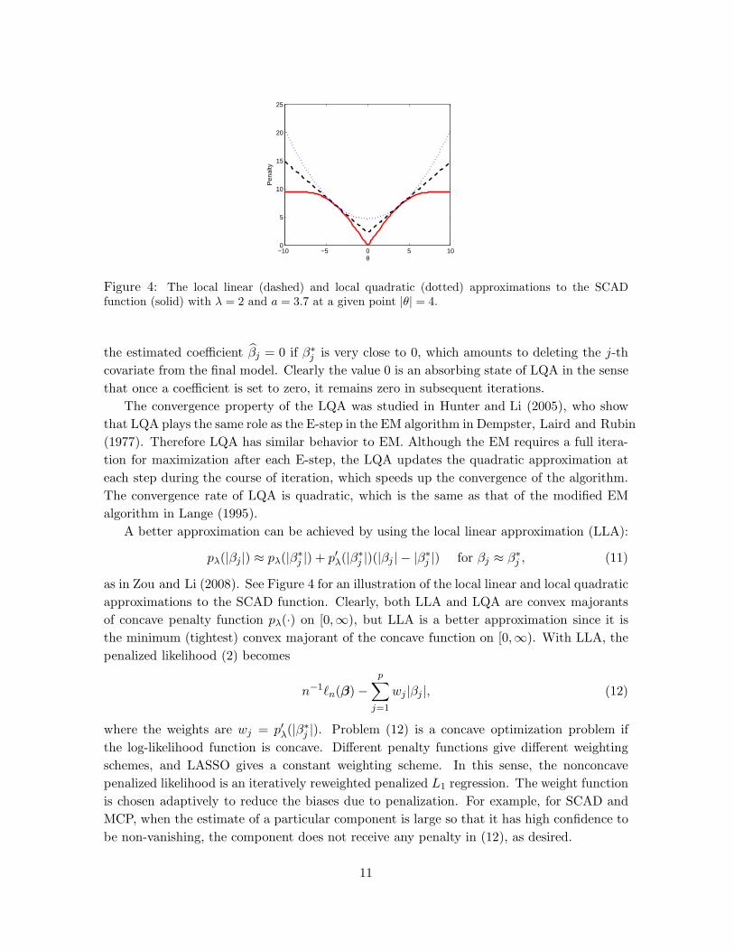
A better approximation can be achieved by using the local linear approximation (LLA):

pλ(|βj |) ≈ pλ(|β∗j |) + p′λ(|β∗j |)(|βj | − |β∗j |) for βj ≈ β∗j , (11)

as in Zou and Li (2008). See Figure 4 for an illustration of the local linear and local quadratic

approximations to the SCAD function. Clearly, both LLA and LQA are convex majorants

of concave penalty function pλ(·) on [0,∞), but LLA is a better approximation since it is

the minimum (tightest) convex majorant of the concave function on [0,∞). With LLA, the

penalized likelihood (2) becomes

n−1ℓn(β) −p∑

j=1

wj |βj |, (12)

where the weights are wj = p′λ(|β∗j |). Problem (12) is a concave optimization problem if

the log-likelihood function is concave. Different penalty functions give different weighting

schemes, and LASSO gives a constant weighting scheme. In this sense, the nonconcave

penalized likelihood is an iteratively reweighted penalized L1 regression. The weight function

is chosen adaptively to reduce the biases due to penalization. For example, for SCAD and

MCP, when the estimate of a particular component is large so that it has high confidence to

be non-vanishing, the component does not receive any penalty in (12), as desired.

11

Zou (2006) proposes the weighting scheme wj = |β∗j |−γ for some γ > 0 and calls the

resulting procedure adaptive LASSO. This weight reduces the penalty when the previous

estimate is large. However, the penalty at zero is infinite. When the procedure is applied

iteratively, zero becomes an absorbing state. On the other hand, the penalty functions such

as SCAD and MCP do not have this undesired property. For example, if the initial estimate

is zero, then wj = λ and the resulting estimate is the LASSO estimate.

Fan and Li (2001), Zou (2006), and Zou and Li (2008) all suggest a consistent estimate

such as the un-penalized MLE. This implicitly assumes that p ≪ n. For dimensionality p

that is larger than sample size n, the above method is not applicable. Fan and Lv (2008)

recommend using β∗j = 0, which is equivalent to using the LASSO estimate as the initial

estimate. Another possible initial value is to use a stepwise addition fit or componentwise

regression. They put forward the recommendation that only a few iterations are needed,

which is in line with Zou and Li (2008).

Before we close this section, we remark that with the LLA and LQA, the resulting

sequence of target values is always nondecreasing, which is a specific feature of minorization-

maximization (MM) algorithms (Hunter and Lange (2000)). Let pλ(β) =∑p

j=1 pλ(|βj |).Suppose that at the k-th iteration, pλ(β) is approximated by qλ(β) such that

pλ(β) ≤ qλ(β) and pλ(β(k)) = qλ(β(k)), (13)

where β(k) is the estimate at the k-th iteration. Let β(k+1) maximize the approximated

penalized likelihood n−1ℓn(β) − qλ(β). Then we have

n−1ℓn(β(k+1)) − pλ(β(k+1)) ≥ n−1ℓn(β(k+1)) − qλ(β(k+1))

≥ n−1ℓn(β(k)) − qλ(β(k))

= n−1ℓn(β(k)) − pλ(β(k)).

Thus, the target values are non-decreasing. Clearly, the LLA and LQA are two specific cases

of the MM algorithms, satisfying condition (13); see Figure 4. Therefore, the sequence of

target function values is non-decreasing and thus converges provided it is bounded. The

critical point is the global maximizer under the conditions in Fan and Lv (2009).

3.4 LARS and other algorithms

As demonstrated in the previous section, the penalized least squares problem (4) with an

L1 penalty is fundamental to the computation of penalized likelihood estimation. There are

several additional powerful algorithms for such an endeavor. Osborne, Presnell and Turlach

(2000) cast such a problem as a quadratic programming problem. Efron et al. (2004) propose

a fast and efficient least angle regression (LARS) algorithm for variable selection, a simple

modification of which produces the entire LASSO solution path {β(λ) : λ > 0} that optimizes

(4). The computation is based on the fact that the LASSO solution path is piecewise linear

in λ. See Rosset and Zhu (2007) for a more general account of the conditions under which

the solution to the penalized likelihood (2) is piecewise linear. The LARS algorithm starts

12

from a large value of λ which selects only one covariate that has the greatest correlation

with the response variable and decreases the λ value until the second variable is selected,

at which the selected variables have the same correlation (in magnitude) with the current

working residual as the first one, and so on. See Efron et al. (2004) for details.

The idea of the LARS algorithm can be expanded to compute the solution paths of

penalized least squares (4). Zhang (2009) introduces the PLUS algorithm for efficiently

computing a solution path of (4) when the penalty function pλ(·) is a quadratic spline such

as the SCAD and MCP. In addition, Zhang (2009) also shows that the solution path β(λ) is

piecewise linear in λ, and the proposed solution path has desired statistical properties.

For the penalized least squares problem (4), Fu (1998), Daubechies, Defrise and De Mol

(2004), and Wu and Lang (2008) propose a coordinate descent algorithm, which iteratively

optimizes (4) one component at a time. This algorithm can also be applied to optimize the

group LASSO (Antoniadis and Fan (2001); Yuan and Lin (2006)) as shown in Meier, van de Geer and Buhlmann

(2008), penalized precision matrix estimation (Friedman, Hastie and Tibshirani (2007)), and

penalized likelihood (2) (Fan and Lv (2009); Zhang and Li (2009)).

More specifically, Fan and Lv (2009) employ a path-following coordinate optimization

algorithm, called the iterative coordinate ascent (ICA) algorithm, for maximizing the non-

concave penalized likelihood. It successively maximizes the penalized likelihood (2) for reg-

ularization parameters λ in decreasing order. A similar idea is also studied in Zhang and Li

(2009), who introduce the ICM algorithm. The coordinate optimization algorithm uses

the Gauss-Seidel method, i.e., maximizing one coordinate at a time with successive dis-

placements. Specifically, for each coordinate within each iteration, it uses the second order

approximation of ℓn(β) at the p-vector from the previous step along that coordinate and

maximizes the univariate penalized quadratic approximation

maxθ∈R

{−1

2(z − θ)2 − Λpλ(|θ|)

}, (14)

where Λ > 0. It updates each coordinate if the maximizer of the corresponding univari-

ate penalized quadratic approximation makes the penalized likelihood (2) strictly increase.

Therefore, the ICA algorithm enjoys the ascent property that the resulting sequence of values

of the penalized likelihood is increasing for a fixed λ. Compared to other algorithms, the

coordinate optimization algorithm is especially appealing for large scale problems with both

n and p large, thanks to its low computational complexity. It is fast to implement when the

univariate problem (14) admits a closed-form solution. This is the case for many commonly

used penalty functions such as SCAD and MCP. In practical implementation, we pick a suf-

ficiently large λmax such that the maximizer of the penalized likelihood (2) with λ = λmax is

0, and a decreasing sequence of regularization parameters. The studies in Fan and Lv (2009)

show that the coordinate optimization works equally well and efficiently for producing the

entire solution paths for concave penalties.

The LLA algorithm for computing penalized likelihood is now available in R at

http://cran.r-project.org/web/packages/SIS/index.html

13

as a function in the SIS package. So is the PLUS algorithm for computing the penalized

least squares estimator with SCAD and MC+ penalties. The Matlab codes are also available

for the ICA algorithm for computing the solution path of the penalized likelihood estimator

and for computing SIS upon request.

3.5 Composite quasi-likelihood

The function ℓn(β) in (2) does not have to be the true likelihood. It can be a quasi-likelihood

or a loss function (Fan, Samworth and Wu (2009)). In most statistical applications, it is of

the form

n−1n∑

i=1

Q(xTi β, yi) −

p∑

j=1

pλ(|βj |), (15)

where Q(xTi β, yi) is the conditional quasi-likelihood of Yi given Xi. It can also be the loss

function of using xTi β to predict yi. In this case, the penalized quasi-likelihood (15) is written

as the minimization of

n−1n∑

i=1

L(xTi β, yi) +

p∑

j=1

pλ(|βj |), (16)

where L is a loss function. For example, the loss function can be a robust loss: L(x, y) =

|y−x|. How should we choose a quasi-likelihood to enhance the efficiency of procedure when

the error distribution possibly deviates from normal?

To illustrate the idea, consider the linear model (3). As long as the error distribution of

ε is homoscedastic, xTi β is, up to an additive constant, the conditional τ quantile of yi given

xi. Therefore, β can be estimated by the quantile regression

n∑

i=1

ρτ (yi − bτ − xTi β),

where ρτ (x) = τx+ + (1 − τ)x− (Koenker and Bassett (1978)). Koenker (1984) proposes

solving the weighted composite quantile regression by using different quantiles to improve

the efficiency, namely, minimizing with respect to b1, · · · , bK and β,

K∑

k=1

wk

n∑

i=1

ρτk(yi − bk − xT

i β), (17)

where {τk} is a given sequence of quantiles and {wk} is a given sequence of weights. Zou and Yuan

(2008) propose the penalized composite quantile with equal weights to improve the efficiency

of the penalized least squares.

Recently, Bradic, Fan and Wang (2009) proposed the more general composite quasi-

likelihoodK∑

k=1

wk

n∑

i=1

Lk(xTi β, yi) +

p∑

j=1

pλ(|βj |). (18)

14

They derive the asymptotic normality of the estimator and choose the weight function to

optimize the asymptotic variance. In this view, it always performs better than a single quasi-

likelihood function. In particular, they study in detail the relative efficiency of the composite

L1-L2 loss and optimal composite quantile loss with the least squares estimator.

Note that the composite likelihood (18) can be regarded as an approximation to the

log-likelihood function via

log f(y|x) = log f(y|xT β) ≈ −K∑

k=1

wkLk(xT β, y)

with∑K

k=1wk = 1. Hence, wk can also be chosen to minimize (18) directly. If the convexity

of the composite likelihood is enforced, we need to impose the additional constraint that all

weights are non-negative.

3.6 Choice of penalty parameters

The choice of penalty parameters is of paramount importance in penalized likelihood esti-

mation. When λ = 0, all variables are selected and the model is even unidentifiable when

p > n. When λ = ∞, if the penalty satisfies limλ→∞ pλ(|θ|) = ∞ for θ 6= 0, then none of the

variables is selected. The interesting cases lie between these two extreme choices.

The above discussion clearly indicates that λ governs the complexity of the selected

model. A large value of λ tends to choose a simple model, whereas a small value of λ inclines

to a complex model. The estimation using a larger value of λ tends to have smaller variance,

whereas the estimation using a smaller value of λ inclines to smaller modeling biases. The

trade-off between the biases and variances yields an optimal choice of λ. This is frequently

done by using a multi-fold cross-validation.

There are relatively few studies on the choice of penalty parameters. In Wang, Li and Tsai

(2007), it is shown that the model selected by generalized cross-validation using the SCAD

penalty contains all important variables, but with nonzero probability includes some unim-

portant variables, and that the model selected by using BIC achieves the model selection

consistency and an oracle property. It is worth to point out that missing some true pre-

dictor causes model misspecification, as does misspecifying the family of distributions. A

semi-Bayesian information criterion (SIC) is proposed by Lv and Liu (2008) to address this

issue for model selection.

4 Ultra-high dimensional variable selection

Variable selection in ultra-high dimensional feature space has become increasingly important

in statistics, and calls for new or extended statistical methodologies and theory. For exam-

ple, in disease classification using microarray gene expression data, the number of arrays is

usually on the order of tens while the number of gene expression profiles is on the order of

tens of thousands; in the study of protein-protein interactions, the number of features can

be on the order of millions while the sample size n can be on the order of thousands (see,

15

d p

SIS

SCADMCP

LASSODS

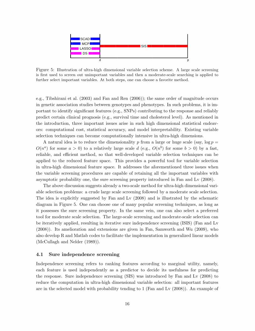
Figure 5: Illustration of ultra-high dimensional variable selection scheme. A large scale screeningis first used to screen out unimportant variables and then a moderate-scale searching is applied tofurther select important variables. At both steps, one can choose a favorite method.

e.g., Tibshirani et al. (2003) and Fan and Ren (2006)); the same order of magnitude occurs

in genetic association studies between genotypes and phenotypes. In such problems, it is im-

portant to identify significant features (e.g., SNPs) contributing to the response and reliably

predict certain clinical prognosis (e.g., survival time and cholesterol level). As mentioned in

the introduction, three important issues arise in such high dimensional statistical endeav-

ors: computational cost, statistical accuracy, and model interpretability. Existing variable

selection techniques can become computationally intensive in ultra-high dimensions.

A natural idea is to reduce the dimensionality p from a large or huge scale (say, log p =

O(na) for some a > 0) to a relatively large scale d (e.g., O(nb) for some b > 0) by a fast,

reliable, and efficient method, so that well-developed variable selection techniques can be

applied to the reduced feature space. This provides a powerful tool for variable selection

in ultra-high dimensional feature space. It addresses the aforementioned three issues when

the variable screening procedures are capable of retaining all the important variables with

asymptotic probability one, the sure screening property introduced in Fan and Lv (2008).

The above discussion suggests already a two-scale method for ultra-high dimensional vari-

able selection problems: a crude large scale screening followed by a moderate scale selection.

The idea is explicitly suggested by Fan and Lv (2008) and is illustrated by the schematic

diagram in Figure 5. One can choose one of many popular screening techniques, as long as

it possesses the sure screening property. In the same vein, one can also select a preferred

tool for moderate scale selection. The large-scale screening and moderate-scale selection can

be iteratively applied, resulting in iterative sure independence screening (ISIS) (Fan and Lv

(2008)). Its amelioration and extensions are given in Fan, Samworth and Wu (2009), who

also develop R and Matlab codes to facilitate the implementation in generalized linear models

(McCullagh and Nelder (1989)).

4.1 Sure independence screening

Independence screening refers to ranking features according to marginal utility, namely,

each feature is used independently as a predictor to decide its usefulness for predicting

the response. Sure independence screening (SIS) was introduced by Fan and Lv (2008) to

reduce the computation in ultra-high dimensional variable selection: all important features

are in the selected model with probability tending to 1 (Fan and Lv (2008)). An example of

16

independence learning is the correlation ranking proposed in Fan and Lv (2008) that ranks

features according to the magnitude of its sample correlation with the response variable.

More precisely, let ω = (ω1, · · · , ωp)T = XTy be a p-vector obtained by componentwise

regression, where we assume that each column of the n × p design matrix X has been

standardized with mean zero and variance one. For any given dn, take the selected submodel

to be

Md = {1 ≤ j ≤ p : |ωj| is among the first dn largest of all}. (19)

This reduces the full model of size p≫ n to a submodel with size dn, which can be less than

n. Such correlation learning screens those variables that have weak marginal correlations

with the response. For classification problems with Y = ±1, the correlation ranking reduces

to selecting features by using two-sample t-test statistics. See Section 4.2 for additional

details.

Other examples of independence learning include methods in microarray data analysis

where a two-sample test is used to select significant genes between the treatment and control

groups (Dudoit, Shaffer and Boldrick (2003); Storey and Tibshirani (2003); Fan and Ren (2006);

Efron (2007)), feature ranking using a generalized correlation (Hall and Miller (2009a)), non-

parametric learning under sparse additive models (Ravikumar et al. (2009)), and the method

in Huang, Horowitz and Ma (2008) that uses the marginal bridge estimators for selecting

variables in high dimensional sparse regression models. Hall, Titterington and Xue (2009)

derive some independence learning rules using tilting methods and empirical likelihood, and

propose a bootstrap method to assess the fidelity of feature ranking. In particular, the false

discovery rate (FDR) proposed by Benjamini and Hochberg (1995) is popularly used in mul-

tiple testing for controlling the expected false positive rate. See also Efron et al. (2001),

Abramovich et al. (2006), Donoho and Jin (2006), and Clarke and Hall (2009).

We now discuss the sure screening property of correlation screening. Let M∗ = {1 ≤ j ≤p : βj 6= 0} be the true underlying sparse model with nonsparsity size s = |M∗|; the other

p−s variables can also be correlated with the response variable via the link to the predictors

in the true model. Fan and Lv (2008) consider the case p ≫ n with log p = O(na) for some

a ∈ (0, 1 − 2κ), where κ is specified below, and Gaussian noise ε ∼ N(0, σ2) for some σ > 0.

They assume that var(Y ) = O(1), λmax(Σ) = O(nτ ),

minj∈M∗

|βj | ≥ cn−κ and minj∈M∗

|cov(β−1j Y,Xj)| ≥ c,

where Σ = cov(x), κ, τ ≥ 0, c is a positive constant, and the p-dimensional covariate

vector x has an elliptical distribution with the random matrix XΣ−1/2 having a concentra-

tion property that holds for Gaussian distributions. For studies on the extreme eigenvalues

and limiting spectral distributions of large random matrices, see, e.g., Silverstein (1985),

Bai and Yin (1993), Bai (1999), Johnstone (2001), and Ledoux (2001, 2005).

Under the above regularity conditions, Fan and Lv (2008) show that if 2κ+ τ < 1, then

there exists some θ ∈ (2κ+ τ, 1) such that when dn ∼ nθ, we have for some C > 0,

P (M∗ ⊂ Md) = 1 −O(pe−Cn1−2κ/ log n). (20)

17

In particular, this sure screening property entails the sparsity of the model: s ≤ dn. It

demonstrates that SIS can reduce exponentially high dimensionality to a relatively large

scale dn ≪ n, while the reduced model Mγ still contains all the important variables with

an overwhelming probability. In practice, to be conservative we can choose d = n − 1 or

[n/ log n]. Of course, one can also take final model size d ≥ n. Clearly larger d means larger

probability of including the true underlying sparse model M∗ in the final model Md. See

Section 4.3 for further results on sure independence screening.

When the dimensionality is reduced from a large scale p to a moderate scale d by applying

a sure screening method such as correlation learning, the well-developed variable selection

techniques, such as penalized least squares methods, can be applied to the reduced feature

space. This is a powerful tool of SIS based variable selection methods. The sampling proper-

ties of these methods can be easily obtained by combining the theory of SIS and penalization

methods.

4.2 Feature selection for classification

Independence learning has also been widely used for feature selection in high dimensional

classification problems. In this section we look at the specific setting of classification and

continue the topic of independence learning for variable selection in Section 4.3. Consider

the p-dimensional classification between two classes. For k ∈ {1, 2}, let Xk1, Xk2, · · · , Xknk

be i.i.d. p-dimensional observations from the k-th class. Classification aims at finding a

discriminant function δ(x) that classifies new observations as accurately as possible. The

classifier δ(·) assigns x to the class 1 if δ(x) ≥ 0 and class 2 otherwise.

Many classification methods have been proposed in the literature. The best classifier is

the Fisher δF (x) = (x − µ)′Σ−1(µ1 − µ2) when the data are from the normal distribution

with a common covariance matrix: Xki ∼ N(µk,Σ), for k = 1, 2 and µ = (µ1 + µ2)/2.

However, this method is hard to implement when dimensionality is high due to the difficulty

of estimating the unknown covariance matrix Σ. Hence, the independence rule that involves

estimating the diagonal entries of the covariance matrix, with discriminant function δ(x) =

(x−µ)′D−1(µ1 −µ2) is frequently employed for the classification, where D = diag{Σ}. For

a survey of recent developments, see Fan, Fan and Wu (2010).

Classical methods break down when the dimensionality is high. As demonstrated by

Bickel and Levina (2004), the Fisher discrimination method no longer performs well in high

dimensional settings due to the diverging spectra and singularity of the sample covariance

matrix. They show that the independence rule overcomes these problems and outperforms

the Fisher discriminant in high dimensional setting. However, in practical implementation

such as tumor classification using microarray data, one hopes to find tens of genes that have

high discriminative power. The independence rule does not possess the property of feature

selection.

The noise accumulation phenomenon is well-known in the regression setup, but has never

been quantified in the classification problem until Fan and Fan (2008). They show that the

difficulty of high dimensional classification is intrinsically caused by the existence of many

18

noise features that do not contribute to the reduction of classification error. For example,

in linear discriminant analysis one needs to estimate the class mean vectors and covariance

matrix. Although each parameter can be estimated accurately, aggregated estimation error

can be very large and can significantly increase the misclassification rate.

Let R0 be the common correlation matrix, λmax(R0) be its largest eigenvalue, and α =

µ1 − µ2. Consider the parameter space

Γ = {(α,Σ) : α′D−1α ≥ Cp, λmax(R0) ≤ b0, min1≤j≤p

σ2j > 0},

where Cp and b0 are given constants, and σ2j is the j-th diagonal element of Σ. Note

that Cp measures the strength of signals. Let δ be the estimated discriminant function

of the independence rule, obtained by plugging in the sample estimates of α and D. If√n1n2/(np)Cp → D0 ≥ 0, Fan and Fan (2008) demonstrate that the worst case classification

error, W (δ), over the parameter space Γ converges:

W (δ)P−→ 1 − Φ

( D0

2√b0

), (21)

where n = n1 + n2 and Φ(·) is the cumulative distribution function of the standard normal

random variable.

The misclassification rate (21) relates to dimensionality in the term D0, which depends

on Cp/√p. This quantifies the tradeoff between dimensionality p and the overall signal

strength Cp. The signal Cp always increases with dimensionality. If the useful features are

located at the first s components, say, then the signals stop increasing when more than

s features are used, yet the penalty of using all features is√p. Clearly, using s features

can perform much better than using all p features. The optimal number should be the one

that minimizes Cm/√m, where the Cm are the signals of the best subset S of m features,

defined as αSD−1S αS, where αS and DS are the sub-vector and sub-matrix of α and D

constructed using variables in S. The result (21) also indicates that the independence rule

works no better than random guessing due to noise accumulation, unless the signal levels are

extremely high, say,√n/pCp ≥ B for some B > 0. Hall, Pittelkow and Ghosh (2008) show

that if C2p/p → ∞, the classification error goes to zero for a distance-based classifier, which

is a specific result of Fan and Fan (2008) with B = ∞.

The above results reveal that dimensionality reduction is also very important for reducing

misclassification rate. A popular class of dimensionality reduction techniques is projection.

See, for example, principal component analysis in Ghosh (2002) and Zou, Hastie and Tibshirani

(2004); partial least squares in Huang and Pan (2003), and Boulesteix (2004); and sliced in-

verse regression in Chiaromonte and Martinelli (2002), Antoniadis, Lambert-Lacroix and Leblanc

(2003), and Bura and Pfeiffer (2003). These projection methods attempt to find directions

that can result in small classification errors. In fact, the directions that they find usually

put much larger weights on features with large classification power, which is indeed a type

of sparsity in the projection vector. Fan and Fan (2008) formally show that linear projec-

tion methods are likely to perform poorly unless the projection vector is sparse, namely, the

19

effective number of selected features is small. This is due to the aforementioned noise accu-

mulation when estimating µ1 and µ2 in high dimensional problems. For formal results, see

Theorem 2 in Fan and Fan (2008). See also Tibshirani et al. (2002), Donoho and Jin (2008),

Hall, Park and Samworth (2008), Hall, Pittelkow and Ghosh (2008), Hall and Chan (2009),

Hall and Miller (2009b), and Jin (2009) for some recent developments in high dimensional

classifications.

To select important features, the two-sample t test is frequently employed (see, e.g.,

Tibshirani et al. (2003)). The two-sample t statistic for feature j is

Tj =X1j − X2j√

S21j/n1 + S2

2j/n2

, j = 1, · · · , p, (22)

where Xkj and S2kj are the sample mean and variance of the j-th feature in class k. This

is a specific example of independence learning, which ranks the features according to |Tj |.Fan and Fan (2008) prove that when dimensionality p grows no faster than the exponential

rate of the sample size, if the lowest signal level is not too small, the two-sample t test can

select all important features with probability tending to 1. Their proof relies on the devia-

tion results of the two-sample t-statistic. See, e.g., Hall (1987, 2006), Jing, Shao and Wang

(2003), and Cao (2007) for large deviation theory.

Although the t test can correctly select all important features with probability tending

to 1 under some regularity conditions, the resulting choice is not necessarily optimal, since

the noise accumulation can exceed the signal accumulation for faint features. Therefore,

it is necessary to further single out the most important features. To address this issue,

Fan and Fan (2008) propose the Features Annealed Independence Rule (FAIR). Instead of

constructing the independence rule using all features, FAIR selects the most important ones

and uses them to construct an independence rule. To appreciate the idea of FAIR, first note

that the relative importance of features can be measured by |αj |/σj , where αj is the j-th

component of α = µ1 − µ2 and σ2j is the common variance of the j-th feature. If such

oracle ranking information is available, then one can construct the independence rule using

m features with the largest |αj |/σj , with optimal value of m to be determined. In this case,

the oracle classifier takes the form

δ(x) =

p∑

j=1

αj(xj − µj)/σ2j 1{|αj |/σj>b},

where b is a positive constant. It is easy to see that choosing the optimal m is equivalent to

selecting the optimal b. However oracle information is usually unavailable, and one needs to

learn it from the data. Observe that |αj |/σj can be estimated by |αj|/σj , where the latter is in

fact√n/(n1n2)|Tj |, in which the pooled sample variance is used. This is indeed the same as

ranking the feature by using the correlation between the jth variable with the class response

±1 when n1 = n2 (Fan and Lv (2008)). Indeed, as pointed out by Hall, Titterington and Xue

(2008), this is always true if the response for the first class is assigned as 1, whereas the

response for the second class is assigned as −n1/n2. Thus to mimick the oracle, FAIR takes

20

a slightly different form to adapt to the unknown signal strength

δFAIR(x) =

p∑

j=1

αj(xj − µj)/σ2j 1{

√n/(n1n2)|Tj |>b}. (23)

It is clear from (23) that FAIR works the same way as if we first sort the features by the

absolute values of their t-statistics in descending order, then take out the first m features to

construct a classifier. The number of features is selected by minimizing the upper bound of

the classification error:

m = arg max1≤m≤p

1

λmmax

n[∑m

j=1 T2(j) +m(n1 − n2)/n]2

mn1n2 + n1n2∑m

j=1 T2(j)

,

where T 2(1) ≥ T 2

(2) ≥ · · · ≥ T 2(p) are the ordered squared t-statistics, and λm

max is the estimate

of the largest eigenvalue of the correlation matrix Rm0 of the m most significant features.

Fan and Fan (2008) also derive the misclassification rates of FAIR and demonstrate that it

possesses an oracle property.

4.3 Sure independence screening for generalized linear models

Correlation learning cannot be directly applied to the case of discrete covariates such as

genetic studies with different genotypes. The mathematical results and technical arguments

in Fan and Lv (2008) rely heavily on the joint normality assumptions. The natural question

is how to screen variables in a more general context, and whether the sure screening property

continues to hold with a limited false positive rate.

Consider the generalized linear model (GLIM) with canonical link. That is, the condi-

tional density is given by

f(y|x) = exp {yθ(x) − b(θ(x)) + c(y)} , (24)

for some known functions b(·), c(·), and θ(x) = xT β. As we consider only variable selection

on the mean regression function, we assume without loss of generality that the dispersion

parameter φ = 1. As before, we assume that each variable has been standardized with mean

0 and variance 1.

For GLIM (24), the penalized likelihood (2) is

− n−1n∑

i=1

ℓ(xTi β, yi) −

p∑

j=1

pλ(|βj |), (25)

where ℓ(θ, y) = b(θ) − yθ. The maximum marginal likelihood estimator (MMLE) βMj is

defined as the minimizer of the componentwise regression

βMj = (βM

j,0, βMj ) = argminβ0,βj

n∑

i=1

ℓ(β0 + βjXij , Yi), (26)

21

where Xij is the ith observation of the jth variable. This can be easily computed and its

implementation is robust, avoiding numerical instability in ultra-high dimensional problems.

The marginal estimator estimates the wrong object of course, but its magnitude provides

useful information for variable screening. Fan and Song (2009) select a set of variables whose

marginal magnitude exceeds a predefined threshold value γn:

Mγn = {1 ≤ j ≤ p : |βMj | ≥ γn}, (27)

This is equivalent to ranking features according to the magnitude of MMLEs {|βMj |}. To

understand the utility of MMLE, we take the population version of the minimizer of the

componentwise regression to be

βMj = (βM

j,0, βMj )T = argminβ0,βj

Eℓ(β0 + βjXj, Y ).

Fan and Song (2009) show that βMj = 0 if and only if cov(Xj , Y ) = 0, and under some

additional conditions if |cov(Xj , Y )| ≥ c1n−κ for j ∈ M⋆, for given positive constants c1 and

κ, then there exists a constant c2 such that

minj∈M⋆

|βMj | ≥ c2n

−κ. (28)

In words, as long asXj and Y are somewhat marginally correlated with κ < 1/2, the marginal

signal βMj is detectable. They prove further the sure screening property:

P(M⋆ ⊂ Mγn

)→ 1 (29)

(the convergence is exponentially fast) if γn = c3n−κ with a sufficiently small c3, and that

only the size of non-sparse elements (not the dimensionality) matters for the purpose of

sure screening property. For the Gaussian linear model (3) with sub-Gaussian covariate

tails, the dimensionality can be as high as log p = o(n(1−2κ)/4), a weaker result than that in

Fan and Lv (2008) in terms of condition on p, but a stronger result in terms of the conditions

on the covariates. For logistic regression with bounded covariates, such as genotypes, the

dimensionality can be as high as log p = o(n1−2κ).

The sure screening property (29) is only part of the story. For example, if γn = 0 then

all variables are selected and hence (29) holds. The question is how large the size of the

selected model size in (27) with γn = c3n−κ should be. Under some regularity conditions,

Fan and Song (2009) show that with probability tending to one exponentially fast,

|Mγn | = O{n2κλmax(Σ)}. (30)

In words, the size of selected model depends on how large the thresholding parameter γn is,

and how correlated the features are. It is of order O(n2κ+τ ) if λmax(Σ) = O(nτ ). This is the

same or somewhat stronger result than in Fan and Lv (2008) in terms of selected model size,

but holds for a much more general class of models. In particularly, there is no restrictions

on κ and τ , or more generally λmax(Σ).

22

Fan and Song (2009) also study feature screening by using the marginal likelihood ratio

test. Let L0 = minβ0n−1

∑ni=1 ℓ(β0, Yi) and

Lj = L0 − minβ0,βjn−1

n∑

i=1

ℓ(β0 + βjXij , Yi). (31)

Rank the features according to the marginal utility {Lj}. Thus, select a set of variables

Nνn = {1 ≤ j ≤ pn : Lj ≥ νn}, (32)

where νn is a predefined threshold value. Let L⋆j be the population counterpart of Lj.

Then, the minimum signal minj∈M∗L⋆

j is of order O(n−2κ), whereas the individual noise

Lj − L⋆j = Op(n

−1/2). In words, when κ ≥ 1/4, the noise level is larger than the signal.

This is the key technical challenge. By using the fact that the ranking is invariant to

monotonic transformations, Fan and Song (2009) are able to show that with νn = c4n−2κ

for a sufficiently small c4 > 0,

P{M∗ ⊂ Nνn , |Nνn | ≤ O(n2κλmax(Σ))} → 1.

Thus the sure screening property holds with a limited size of the selected model.

4.4 Reduction of false positive rate

A screening method is usually a crude approach that results in many false positive variables.

A simple idea of reducing the false positive rate is to apply a resampling technique as proposed

by Fan, Samworth and Wu (2009). Split the samples randomly into two halves and let A1

and A2 be the selected sets of active variables based on, respectively, the first half and the

second half of the sample. If A1 and A2 both have a sure screening property, so does the

set A. On the other hand, A = A1 ∩ A2 has many fewer falsely selected variables, as an

unimportant variable has to be selected twice at random in the ultra-high dimensional space,

which is very unlikely. Therefore, A reduces the number of false positive variables.

Write A for the set of active indices – that is, the set containing those indices j for which

βj 6= 0 in the true model. Let d be the size of the selected sets A1 and A2. Under some

exchangeability conditions, Fan, Samworth and Wu (2009) demonstrate that

P (|A ∩ Ac| ≥ r) ≤(dr

)2

(p−|A|r

) ≤ 1

r!

( n2

p− |A|)r, (33)

where, for the second inequality, we require that d ≤ n ≤ (p − |A|)1/2. In other words, the

probability of selecting at least r inactive variables is very small when n is small compared

to p, such as for the situations discussed in the previous two sections.

4.5 Iterative sure independence screening

SIS uses only the marginal information of the covariates and its sure screening property can

fail when technical conditions are not satisfied. Fan and Lv (2008) point out three potential

problems with SIS:

23

a) (False Negative) An important predictor that is marginally uncorrelated but jointly

correlated with the response cannot be picked by SIS. An example of this has the

covariate vector x jointly normal with equi-correlation ρ, while Y depends on the

covariates through

xT β⋆ = X1 + · · · +XJ − JρXJ+1.

Clearly, XJ+1 is independent of xT β⋆ and hence Y , yet the regression coefficient −Jρcan be much larger than for other variables. Such a hidden signature variable cannot

be picked by using independence learning, but it has a dominant predictive power on

Y .

b) (False Positive) Unimportant predictors that are highly correlated with the important

predictors can have higher priority to be selected by SIS than important predictors

that are relatively weakly related to the response. An illustrative example has

Y = ρX0 +X1 + · · · +XJ + ε,

where X0 is independent of the other variables which have a common correlation ρ.

Then corr(Xj , Y ) = Jρ = J corr(X0, Y ), for j = J + 1, · · · , p, and X0 has the lowest

priority to be selected.

c) The issue of collinearity among the predictors adds difficulty to the problem of variable

selection.

Translating a) to microarray data analysis, a two-sample test can never pick up a hidden

signature gene. Yet, missing the hidden signature gene can result in very poor understanding

of the molecular mechanism and in poor disease classification. Fan and Lv (2008) address

these issues by proposing an iterative SIS (ISIS) that extends SIS and uses more fully the

joint information of the covariates. ISIS still maintains computational expediency.

Fan, Samworth and Wu (2009) extend and improve the idea of ISIS from the multiple

regression model to the more general loss function (16); this includes, in addition to the

log-likelihood, the hinge loss L(x, y) = (1−xy)+ and exponential loss L(x, y) = exp(−xy) in

classification in which y takes values ±1, among others. The ψ-learning (Shen et al. (2003))

can also be cast in this framework. ISIS also allows variable deletion in the process of

iteration. More generally, suppose that our objective is to find a sparse β to minimize

n−1n∑

i=1

L(Yi,xTi β) +

p∑

j=1

pλ(|βj |).

The algorithm goes as follows.

1. Apply an SIS such as (32) to pick a set A1 of indices of size k1, and then employ a

penalized (pseudo)-likelihood method (15) to select a subset M1 of these indices.

24

2. (Large-scale screening) Instead of computing residuals as in Fan and Lv (2008), com-

pute

L(2)j = min

β0,βM1,βj

n−1n∑

i=1

L(Yi, β0 + xTi,M1

βM1+Xijβj), (34)

for j 6∈ M1, where xi,M1is the sub-vector of xi consisting of those elements in M1.

This measures the additional contribution of variable Xj in the presence of variables

xM1. Pick k2 variables with the smallest {L(2)

j , j 6∈ M1} and let A2 be the resulting

set.

3. (Moderate-scale selection) Use penalized likelihood to obtain

β2 = argminβ0,βM1,βA2

n−1n∑

i=1

L(Yi, β0 + xTi,M1

βM1+ xT

i,A2βA2

) +∑

j∈M1∪A2

pλ(|βj |).

(35)

This gives new active indices M2 consisting of nonvanishing elements of β2. This step

also deviates importantly from the approach in Fan and Lv (2008) even in the least

squares case. It allows the procedure to delete variables from the previous selected

variables M1.

4. (Iteration) Iterate the above two steps until d (a prescribed number) variables are

recruited or Mℓ = Mℓ−1.

The final estimate is then βMℓ. In implementation, Fan, Samworth and Wu (2009) choose

k1 = ⌊2d/3⌋, and thereafter at the r-th iteration, take kr = d − |Mr−1|. This ensures that

the iterated versions of SIS take at least two iterations to terminate. The above method

can be considered as an analogue of the least squares ISIS procedure (Fan and Lv (2008))

without explicit definition of the residuals. Fan and Lv (2008) and Fan, Samworth and Wu

(2009) show empirically that the ISIS significantly improves the performance of SIS even in

the difficult cases described above.

5 Sampling properties of penalized least squares

The sampling properties of penalized likelihood estimation (2) have been extensively stud-

ied, and a significant amount of work has been contributed to penalized least squares (4).

The theoretical studies can be mainly classified into four groups: persistence, consistency

and selection consistency, the weak oracle property, and the oracle property (from weak to

strong). Again, persistence means consistency of the risk (expected loss) of the estimated

model, as opposed to consistency of the estimate of the parameter vector under some loss.

Selection consistency means consistency of the selected model. By the weak oracle property,

we mean that the estimator enjoys the same sparsity as the oracle estimator with asymp-

totic probability one, and has consistency. The oracle property is stronger than the weak

oracle property in that, in addition to the sparsity in the same sense and consistency, the

estimator attains an information bound mimicking that of the oracle estimator. Results have

25

revealed the behavior of different penalty functions and the impact of dimensionality on high

dimensional variable selection.

5.1 Dantzig selector and its asymptotic equivalence to LASSO

The L1 regularization (e.g., LASSO) has received much attention due to its convexity

and encouraging sparsity solutions. The idea of using the L1 norm can be traced back

to the introduction of convex relaxation for deconvolution in Claerbout and Muir (1973),

Taylor, Banks and McCoy (1979), and Santosa and Symes (1986). The use of the L1 penalty

has been shown to have close connections to other methods. For example, sparse approxi-

mation using an L1 approach is shown in Girosi (1998) to be equivalent to support vector

machines (Vapnik (1995)) for noiseless data. Another example is the asymptotic equivalence

between the Dantzig selector (Candes and Tao (2007)) and LASSO.

The L1 regularization has also been used in the Dantzig selector recently proposed by

Candes and Tao (2007), which is defined as the solution to

min ‖β‖1 subject to ‖n−1XT (y − Xβ)‖∞ ≤ λ, (36)

where λ ≥ 0 is a regularization parameter. It was named after Dantzig because the convex

optimization problem (36) can easily be recast as a linear program. Unlike the PLS (4) which

uses the residual sum of squares as a measure of goodness of fit, the Dantzig selector uses the

L∞ norm of the covariance vector n−1XT (y − Xβ), i.e., the maximum absolute covariance

between a covariate and the residual vector y − Xβ, for controlling the model fitting. This

L∞ constraint can be viewed as a relaxation of the normal equation

XTy = XTXβ, (37)

namely, finding the estimator that has the smallest L1-norm in the neighborhood of the

least squares estimate. A prominent feature of the Dantzig selector is its nonasymptotic

oracle inequalities under L2 loss. Consider the Gaussian linear regression model (3) with

ε ∼ N(0, σ2In) for some σ > 0, and assume that each covariate is standardized to have L2

norm√n (note that we changed the scale of X since it was assumed that each covariate has

unit L2 norm in Candes and Tao (2007)). Under the uniform uncertainty principle (UUP)

on the design matrix X, a condition on the finite condition number for submatrices of X,

they show that, with high probability, the Dantzig selector β mimics the risk of the oracle

estimator up to a logarithmic factor log p, specifically

‖β − β0‖2 ≤ C√

(2 log p)/n(σ2 +∑

j∈supp(β0)β2

0,j ∧ σ2)1/2, (38)

where β0 = (β0,1, · · · , β0,p)T is the vector of the true regression coefficients, C is some

positive constant, and λ ∼√

(2 log p)/n. Roughly speaking, the UUP condition (see also

Donoho and Stark (1989); Donoho and Huo (2001)) requires that all n × d submatrices of

X with d comparable to ‖β0‖0 are uniformly close to orthonormal matrices, which can

be stringent in high dimensions. See Fan and Lv (2008) and Cai and Lv (2007) for more

discussions. The oracle inequality (38) does not infer much about the sparsity of the estimate.

26

Shortly after the work on the Dantzig selector, it was observed that the Dantzig selector

and the LASSO share some similarities. Bickel, Ritov and Tsybakov (2008) present a theo-

retical comparison of the LASSO and the Dantzig selector in the general high dimensional

nonparametric regression model. Under a sparsity scenario, Bickel, Ritov and Tsybakov

(2008) derive parallel oracle inequalities for the prediction risk for both methods, and es-

tablish the asymptotic equivalence of the LASSO estimator and the Dantzig selector. More

specifically, consider the nonparametric regression model

y = f + ε, (39)

where f = (f(x1), · · · , f(xn))T with f an unknown p-variate function, and y, X = (x1, · · · ,xn)T ,

and ε are the same as in (3). Let {f1, · · · , fM} be a finite dictionary of p-variate func-

tions. As pointed out in Bickel, Ritov and Tsybakov (2008), fj’s can be a collection of basis

functions for approximating f , or estimators arising from M different methods. For any

β = (β1, · · · , βM )T , define fβ =∑M

j=1 βjfj. Then similarly to (4) and (36), the LASSO

estimator fL and Dantzig selector fD can be defined accordingly as f bβL

and f bβD

with βL

and βD the corresponding M -vectors of minimizers. In both formations, the empirical norm

‖fj‖n =√n−1

∑ni=1 f

2j (xi) of fj is incorporated as its scale. Bickel, Ritov and Tsybakov

(2008) show that under the restricted eigenvalue condition on the Gram matrix and some

other regularity conditions, with significant probability, the difference between ‖fD − f‖2n

and ‖fL − f‖2n is bounded by a product of three factors. The first factor sσ2/n corresponds

to the prediction error rate in regression with s parameters, and the other two factors in-

cluding logM reflect the impact of a large number of regressors. They further prove sparsity

oracle inequalities for the prediction loss of both estimators. These inequalities entail that

the distance between the prediction losses of the Dantzig selector and the LASSO estimator

is of the same order as the distances between them and their oracle approximations.

Bickel, Ritov and Tsybakov (2008) also consider the specific case of a linear model (3),

say (39) with true regression function f = Xβ0. If ε ∼ N(0, σ2In) and some regularity

conditions hold, they show that, with large probability, the Lq estimation loss for 1 ≤ q ≤ 2

of the Dantzig selector βD is simultaneously given by

‖βD − β0‖qq ≤ Cσq

(1 +

√s/m

)2(q−1)s

(log p

n

)q/2

, (40)

where s = ‖β0‖0, m ≥ s is associated with the strong restricted eigenvalue condition on the

design matrix X, and C is some positive constant. When q = 1, they prove (40) under a

(weak) restricted eigenvalue condition that does not involve m. Bickel, Ritov and Tsybakov

(2008) also derive similar inequalities to (40) with slightly different constants on the Lq

estimation loss, for 1 ≤ q ≤ 2, of the LASSO estimator βL. These results demonstrate the

approximate equivalence of the Dantzig selector and the LASSO. The similarity between the

Dantzig selector and LASSO has also been discussed in Efron, Hastie and Tibshirani (2007).

Lounici (2008) derives the L∞ convergence rate and studies a sign concentration property

27

simultaneously for the LASSO estimator and the Dantzig selector under a mutual coherence

condition.

Note that the covariance vector n−1XT (y − Xβ) in the formulation of Dantzig selector

(36) is exactly the negative gradient of (2n)−1‖y−Xβ‖2 in PLS (4). This in fact entails that

the Dantzig selector and the LASSO estimator are identical under some suitable conditions,

provided that the same regularization parameter λ is used in both methods. For exam-

ple, Meinshausen, Rocha and Yu (2007) give a diagonal dominance condition of the p × p

matrix (XTX)−1 that ensures their equivalence. This condition implicitly assumes p ≤ n.

James, Radchenko and Lv (2009) present a formal necessary and sufficient condition, as well

as easily verifiable sufficient conditions ensuring the identical solution of the Dantzig selector

and the LASSO estimator when the dimensionality p can exceed sample size n.

5.2 Model selection consistency of LASSO

There is a huge literature devoted to studying the statistical properties of LASSO and re-

lated methods. This L1 method as well as its variants have also been extensively stud-

ied in such other areas as compressed sensing. For example, Greenshtein and Ritov (2004)

show that under some regularity conditions the LASSO-type procedures are persistent un-

der quadratic loss for dimensionality of polynomial growth, and Greenshtein (2006) extends

the results to more general loss functions. Meinshausen (2007) presents similar results for

the LASSO for dimensionality of exponential growth and finite nonsparsity size, but its

persistency rate is slower than that of a relaxed LASSO. For consistency and selection

consistency results see Donoho, Elad and Temlyakov (2006), Meinshausen and Buhlmann

(2006), Wainwright (2006), Zhao and Yu (2006), Bunea, Tsybakov and Wegkamp (2007),

Bickel, Ritov and Tsybakov (2008), van de Geer (2008), and Zhang and Huang (2008), among

others.

As mentioned in the previous section, consistency results for the LASSO hold under

some conditions on the design matrix. For the purpose of variable selection, we are also

concerned with the sparsity of the estimator, particularly its model selection consistency

meaning that the estimator β has the same support as the true regression coefficients vector

β0 with asymptotic probability one. Zhao and Yu (2006) characterize the model selection

consistency of the LASSO by studying a stronger but technically more convenient property

of sign consistency: P (sgn(β) = sgn(β0)) → 1 as n → ∞. They show that the weak

irrepresentable condition

‖XT2 X1(X

T1 X1)

−1sgn(β1)‖∞ < 1 (41)

is necessary for sign consistency of the LASSO, and the strong irrepresentable condition,

which requires that the left-hand side of (41) be uniformly bounded by a positive constant

C < 1, is sufficient for sign consistency of the LASSO, where β1 is the subvector of β0 on its

support supp(β0), and X1 and X2 denote the submatrices of the n×p design matrix X formed

by columns in supp(β0) and its complement, respectively. See also Zou (2006) for the fixed

p case. However, the irrepresentable condition can become restrictive in high dimensions.

See Section 5.5 for a simple illustrative example, because the same condition shows up in

28

a related problem of sparse recovery by using L1 regularization. This demonstrates that in

high dimensions, the LASSO estimator can easily select an inconsistent model, which explains

why the LASSO tends to include many false positive variables in the selected model.

To establish the weak oracle property of the LASSO, in addition to the sparsity charac-

terized above, we need its consistency. To this end, we usually need the condition on the

design matrix that

‖XT2 X1(X

T1 X1)

−1‖∞ ≤ C (42)

for some positive constant C < 1, which is stronger than the strong irrepresentable condition.

It says that the L1-norm of the regression coefficients of each inactive variable regressed on

s active variables must be uniformly bounded by C < 1. This shows that the capacity of the

LASSO for selecting a consistent model is very limited, noticing also that the L1-norm of the

regression coefficients typically increase with s. See, e.g., Wainwright (2006). As discussed

above, condition (42) is a stringent condition in high dimensions for the LASSO estimator

to enjoy the weak oracle property. The model selection consistency of the LASSO in the

context of graphical models has been studied by Meinshausen and Buhlmann (2006), who

consider Gaussian graphical models with polynomially growing numbers of nodes.

5.3 Oracle property

What are the sampling properties of penalized least squares (4) and penalized likelihood

estimation (2) when the penalty function pλ is no longer convex? The oracle property

(Fan and Li (2001)) provides a nice conceptual framework for understanding the statistical

properties of high dimensional variable selection methods.

In a seminal paper, Fan and Li (2001) build the theoretical foundation of nonconvex

penalized least squares or, more generally, nonconcave penalized likelihood for variable se-

lection. They introduce the oracle property for model selection. An estimator β is said to

have the oracle property if it enjoys sparsity in the sense that β2 = 0 with probability tending

to 1 as n→ ∞, and β1 attains an information bound mimicking that of the oracle estimator,

where β1 and β2 are the subvectors of β formed by components in supp(β0) and supp(β0)c,

respectively, while the oracle knows the true model supp(β0) beforehand. The oracle proper-

ties of penalized least squares estimators can be understood in the more general framework of

penalized likelihood estimation. Fan and Li (2001) study the oracle properties of nonconcave

penalized likelihood estimators in the finite-dimensional setting, and Fan and Peng (2004)

extend their results to the moderate dimensional setting with p = o(n1/5) or o(n1/3).

More specifically, without loss of generality, assume that the true regression coefficients

vector is β0 = (βT1 ,β

T2 )T with β1 and β2 the subvectors of nonsparse and sparse elements

respectively: ‖β1‖0 = ‖β0‖0 and β2 = 0. Let an = ‖p′λ(|β1|)‖∞ and bn = ‖p′′λ(|β1|)‖∞.

Fan and Li (2001) and Fan and Peng (2004) show that, as long as an, bn = o(1), under some

regularity conditions there exists a local maximizer β to the penalized likelihood (2) such

that

‖β − β0‖2 = OP (√p(n−1/2 + an)). (43)

29

This entails that choosing the regularization parameter λ with an = O(n−1/2) gives a root-

(n/p) consistent penalized likelihood estimator. In particular, this is the case when the

SCAD penalty is used if λ = o(min1≤j≤s |β0,j |), where β1 = (β0,1, · · · , β0,s)T . Recently,

Fan and Lv (2009) gave a sufficient condition under which the solution is unique.

Fan and Li (2001) and Fan and Peng (2004) further prove the oracle properties of penal-

ized likelihood estimators under some additional regularity conditions. Let Σ = diag{p′′λ(|β1|)}and pλ(β1) = sgn(β1) ◦ p′λ(|β1|), where ◦ denotes the the Hadamard (componentwise) prod-

uct. Assume that λ = o(min1≤j≤s |β0,j |),√n/pλ→ ∞ as n→ ∞, and the penalty function

pλ satisfies lim infn→∞ lim inft→0+ p′λ(t)/λ > 0. They show that if p = o(n1/5), then with

probability tending to 1 as n→ ∞, the root-(n/p) consistent local maximizer β = (βT

1 , βT

2 )T

satisfies the following

a) (Sparsity) β2 = 0;

b) (Asymptotic normality)

√nAnI

−1/21 (I1 + Σ)[β1 − β1 + (I1 + Σ)−1pλ(β1)]

D−→ N(0,G), (44)

where An is a q×s matrix such that AnATn → G, a q×q symmetric positive definite matrix,

I1 = I(β1) is the Fisher information matrix knowing the true model supp(β0), and β1 is a

subvector of β formed by components in supp(β0).

Consider a few penalties. For the SCAD penalty, the condition λ = o(min |β1|) entails

that both pλ(β1) and Σ vanish asymptotically. Therefore, the asymptotic normality (44)

becomes √nAnI

1/21 (β1 − β1)

D−→ N(0,G), (45)

which shows that β1 has the same asymptotic efficiency as the MLE of β1 knowing the true

model in advance. This demonstrates that the resulting penalized likelihood estimator is as

efficient as the oracle one. For the L1 penalty (LASSO), the root-(n/p) consistency of β

requires λ = an = O(n−1/2), whereas the oracle property requires√n/pλ → ∞ as n → ∞.

However, these two conditions are incompatible, which suggests that the LASSO estimator

generally does not have the oracle property. This is intrinsically due to the fact that the L1

penalty does not satisfy the unbiasedness condition.

It has indeed been shown in Zou (2006) that the LASSO estimator does not have the

oracle property even in the finite parameter setting. To address the bias issue of LASSO, he

proposes the adaptive LASSO by using an adaptively weighted L1 penalty. More specifically,

the weight vector is |β|−γ for some γ > 0 with the power understood componentwise, where β

is an initial root-n consistent estimator of β0. Since β is root-n consistent, the constructed

weights can separate important variables from unimportant ones. This is an attempt to

introduce the SCAD-like penalty to reduce the biases. From (12), it can easily be seen that

the adaptive LASSO is just a specific solution to penalized least squares using LLA. As a

consequence, Zou (2006) shows that the adaptive LASSO has the oracle property under some

regularity conditions. See also Zhang and Huang (2008).

30

5.4 Additional properties of SCAD estimator

In addition to the oracle properties outlined in the last section and also in Section 6.2,

Kim, Choi and Oh (2008) and Kim and Kwon (2009) provide insights into the SCAD es-

timator. They attempt to answer the question of when the oracle estimator βo

is a local

minimizer of the penalized least squares with the SCAD penalty, when the SCAD estima-

tor and the oracle estimator coincide, and how to check whether a local minimizer is a

global minimizer. The first two results are indeed stronger than the oracle property as they

show that the SCAD estimator is the oracle estimator itself rather than just mimicking its

performance.

Recall that all covariates have been standardized. The follow assumption is needed.

Condition A: The nonsparsity size is sn = O(nc1) for some 0 < c1 < 1, the minimum

eignvalue of the correlation matrix of those active variables is bounded away from zero,

and the minimum signal min1≤j≤sn |βj | > c3n−(1−c2)/2 for some constant c2 ∈ (c1, 1].

Under Condition A, Kim, Choi and Oh (2008) prove that if Eε2ki < ∞ for the linear model

(3),

P (βo

is a local minima of PLS with the SCAD penalty) → 1, (46)

provided that λn = o(n−{1−(c2−c1)}/2) and pn = o{(√nλn)2k}. This shows that the SCAD

method produces the oracle estimator. When k is sufficiently large, the dimensionality

pn can be of any polynomial order. For the Gaussian error, the result holds even with

NP-dimensionality. More precisely, for the Gaussian errors, they show that (46) holds for

pn = O(exp(c4n)) and λn = O(n−(1−c5)/2), where 0 < c4 < c5 < c2 − c1. The question

then arises naturally whether the global minimizer of penalized least squares with the SCAD

penalty is the oracle estimator. Kim, Choi and Oh (2008) give an affirmative answer: with

probability tending to one, the global minimizer of penalized least squares with the SCAD

penalty is the same as the oracle estimator when the correlation matrix of all covariates is

bounded away from zero and infinity (necessarily, pn ≤ n).

Kim and Kwon (2009) also give a simple condition under which the SCAD estimator is

unique and is a global minimizer (see also the simple conditions in Fan and Lv (2009) for

a more general problem). They also provide sufficient conditions to check whether a local

minimizer is a global minimizer. They show that the SCAD method produces the oracle

estimator,

P{The SCAD estimator = βo} → 1,

under conditions similar to Condition A, even when the minimum eigenvalue of the correla-

tion matrix of all variables converges to zero.

5.5 Sparse recovery and compressed sensing

Penalized L1 methods have been widely applied in areas including compressed sensing

(Donoho (2006a)). In those applications, we want to find good sparse representations or

31

approximations of signals that can greatly improve efficiency of data storage and transmis-

sion. We have no intent here to survey results on compressed sensing. Rather, we would

like to make some innate connections of the problem of sparse recovery in the noiseless case

to model selection. Unveiling the role of penalty functions in sparse recovery can give a

simplified view of the role of penalty functions in high dimensional variable selection as the

noise level approaches zero. In particular, we see that concave penalties are advantageous in

sparse recovery, which is in line with the advocation of folded concave penalties for variable

selection as in Fan and Li (2001).

Consider the noiseless case y = Xβ0 of the linear model (3). The problem of sparse

recovery aims to find the sparsest possible solution

arg min ‖β‖0 subject to y = Xβ. (47)

The solution to y = Xβ is not unique when the n × p matrix X has rank less than p, e.g.,

when p > n. See Donoho and Elad (2003) for a characterization of the identifiability of

the minimum L0 solution β0. Although by its nature, the L0 penalty is the target penalty

for sparse recovery, its computational complexity makes it infeasible to implement in high

dimensions. This motivated the use of penalties that are computationally tractable relax-

ations or approximations to the L0 penalty. In particular, the convex L1 penalty provides

a nice convex relaxation and has attracted much attention. For properties of various L1

and related methods see, for example, the Basis Pursuit in Chen, Donoho and Saunders

(1999), Donoho and Elad (2003), Donoho (2004), Fuchs (2004), Candes and Tao (2005,

2006), Donoho, Elad and Temlyakov (2006), Tropp (2006), Candes, Wakin and Boyd (2008),

and Cai, Xu and Zhang (2009).

More generally, we can replace the L0 penalty in (47) by a penalty function ρ(·) and

consider the ρ-regularization problem

min

p∑

j=1

ρ(|βj |) subject to y = Xβ. (48)

This constrained optimization problem is closely related to the PLS in (4). A great deal

of research has contributed to identifying conditions on X and β0 that ensure the L1/L0

equivalence, i.e., the L1-regularization (48) gives the same solution β0. For example, Donoho

(2004) contains deep results and shows that the individual equivalence of L1/L0 depends only

on supp(β0) and β0 on its support. See also Donoho and Huo (2001) and Donoho (2006b).

In a recent work, Lv and Fan (2009) present a sufficient condition that ensures the ρ/L0

equivalence for concave penalties. They consider increasing and concave penalty functions

ρ(·) with finite maximum concavity (curvature). The convex L1 penalty falls at the boundary

of this class of penalty functions. Under these regularity conditions, they show that β0 is a

local minimizer of (48) if there exists some ǫ ∈ (0,minj≤s |β0,j |) such that

maxu∈Uǫ

‖XT2 X1(X

T1 X1)

−1u‖∞ < ρ′(0+), (49)

where Uǫ = {sgn(β1) ◦ ρ′(|v|) : ‖v− β1‖∞ ≤ ǫ}, the notation being that of the previous two

sections.

32

When the L1 penalty is used, Uǫ contains a single point sgn(β1) with sgn understood

componentwise. In this case, condition (49) becomes the weak irrepresentable condition (41).

In fact the L1/L0 equivalence holds provided that (41) weakened to nonstrict inequality is

satisfied. However, this condition can become restrictive in high dimensions. To appreciate

this, look at an example given in Lv and Fan (2009). Suppose that X1 = (x1, · · · ,xs) is

orthonormal, y =∑s

j=1 β0,jxj with |β0,1| = · · · = |β0,s|, xs+1 has unit L2 norm and corre-

lation r with y, and all the rest of the xj ’s are orthogonal to {xj}sj=1. The above condition

becomes |r| ≤ s−1/2. This demonstrates that the L1 penalty can fail to recover the sparsest

solution β0 when the maximum correlation of the noise variable and response is moderately

high, which, as explained in the Introduction, can easily happen in high dimensions.

On the other hand, the concavity of the penalty function ρ entails that its derivative

ρ′(t) is deceasing in t ∈ [0,∞). Therefore, condition (49) can be (much) less restrictive for

concave penalties other than L1. This shows the advantage of concave penalties in sparse

recovery, which is consistent with similar understandings in variable selection in Fan and Li

(2001).

6 Oracle property of penalized likelihood with ultra-high di-

mensionality

As shown in Section 4, large-scale screening and moderate-scale selection is a good strategy

for variable selection in ultra-high dimensional feature spaces. A less stringent screening (i.e.,

a larger selected model size in (24)) will have a higher probability of retaining all important

variables. It is important to study the limits of the dimensionality that nonconcave penalized

likelihood methods can handle. The existing result of Fan and Peng (2004) is too weak in

terms of the dimensionality allowed for high dimensional modeling; they deal with too broad

a class of models.

What are the roles of the dimensionality p and nonsparsity size s? What is the role

of penalty functions? Does the oracle property continue to hold in ultra-high dimensional

feature spaces? These questions have been driving the theoretical development of high di-

mensional variable selection. For example, Koltchinskii (2008) obtains oracle inequalities

for penalized least squares with entropy penalization, and van de Geer (2008) establishes a

nonasymptotic oracle inequality for the Lasso estimator as the empirical risk minimizer in

high dimensional generalized linear models. There are relatively few studies on the statis-

tical properties of high dimensional variable selection methods by using regularization with

nonconvex penalties. More recent studies on this topic include Huang, Horowitz and Ma

(2008), Kim, Choi and Oh (2008), Meier, van de Geer and Buhlmann (2008), Lv and Fan

(2009), Zhang (2009), and Fan and Lv (2009), among others.

6.1 Weak oracle property

An important step towards the understanding of the oracle property of penalized likelihood

methods in ultra-high dimensions is the weak oracle property for model selection, introduced

33

by Lv and Fan (2009) in the context of penalized least squares. An estimator β is said to

have the weak oracle property if it is uniformly consistent and enjoys sparsity in the sense

of β2 = 0 with probability tending to 1, i.e. model selection consistency, where β2 is

the subvector of β formed by components in supp(β0)c and the oracle knows the true model

supp(β0) beforehand. This property is weaker than the oracle property in Fan and Li (2001).

Consistency is derived under L∞ loss, mainly due to the technical difficulty of proving the

existence of a solution to the nonlinear equation that characterizes the nonconcave penalized

likelihood estimator. It is important to study the rate of the probability bound for sparsity

and the rate of convergence for consistency. The dimensionality p usually enters the former

rate explicitly, from which we can see the allowable growth rate of p with sample size n.

Consider the PLS problem (4) with penalty function pλ. Let ρ(t;λ) = λ−1pλ(t) and write

it as ρ(t) whenever there is no confusion. Lv and Fan (2009) and Fan and Lv (2009) consider

the following class of penalty functions:

• ρ(t;λ) is increasing and concave in t ∈ [0,∞), and has a continuous derivative ρ′(t;λ)

with ρ′(0+;λ) > 0. In addition, ρ′(t;λ) is increasing in λ ∈ (0,∞) and ρ′(0+;λ) is

independent of λ.

This is a wide class of concave penalties including SCAD and MCP, and the L1 penalty at

its boundary. Lv and Fan (2009) establish a nonasymptotic weak oracle property for the

PLS estimator. They consider (3) with ε ∼ N(0, σ2In). The notation here is the same as in

Section 5. Assume that each column of the n×p design matrix X (covariate) is standardized

to have L2 norm√n (or of this order), and let dn = 2−1 min {|β0,j | : β0,j 6= 0} be the minimal

signal. The following condition is imposed on the design matrix

‖XT2 X1(X

T1 X1)

−1‖∞ ≤ min(Cρ′(0+)

ρ′(dn), O(nα1)) (50)

where α1 ≥ 0, C ∈ (0, 1), and ρ is associated with the regularization parameter λ ∼nα1−1/2un. Here {un} is a sequence of positive numbers diverging to infinity. Clearly, for

the L1 penalty, condition (50) becomes (42) which is a somewhat stronger form of the strong

irrepresentable condition in Zhao and Yu (2006). Condition (50) consists of two parts: the

first part is intrinsic to the penalty function whereas the second part is purely a technical

condition. For folded-concave penalties other than L1, the intrinsic condition is much more

relaxed: the intrinsic upper bound is C < 1 for the L1 penalty whereas it is ∞ when dn ≫ λn

for the SCAD type of penalty. In other words, the capacity for LASSO to have model se-

lection consistency is limited, independent of model signals, whereas no limit is imposed for

SCAD type of penalties when the signals are strong enough. In general, the concavity of ρ(·)guarantees condition (50) and is more relaxed than the L1 penalty.

Under the above and some additional regularity conditions, if ‖(n−1XT1 X1)

−1‖∞ =

O(nα0) for some α0 ≥ 0, Lv and Fan (2009) show that for sufficiently large n, with proba-

bility at least 1 − 2√πpu−1

n e−u2n/2, the PLS estimator β = (β

T

1 , βT

2 )T satisfies the following

a) (Sparsity) β2 = 0;

34

b) (L∞ loss) ‖β1 − β1‖∞ = O(nα0−1/2un),

where β1 is a subvector of β formed by components in supp(β0). In particular, when the

signals are so sparse that s is finite, α0 = 0 for all non-degenerate problems. In this case,

by taking u2n = c log p for c ≥ 2 so that the probability 1 − 2√

πpu−1

n e−u2n/2 → 1, we have

‖β1 − β1‖∞ = OP (n−1/2√

log p). As an easy consequence of the general result,

‖β − β0‖2 = OP (√snα0−1/2un) (51)

when p = o(uneu2

n/2). The dimensionality p is allowed to grow up to exponentially fast

with un. More specifically, un can be allowed as large as o(n1/2−α0−α1dn) and thus log p =

o(n1−2(α0+α1)d2n). This shows that a weaker minimal signal needs slower growth of dimen-

sionality for successful variable selection. From their studies, we also see the known fact that

concave penalties can reduce the biases of estimates.

Recently, Fan and Lv (2009) extended the results of Lv and Fan (2009) and established

a nonasymptotic weak oracle property for non-concave penalized likelihood estimator in

generalized linear models with ultra-high dimensionality. In their weak oracle property, they

relax the term un from the consistency rate. A similar condition to (50) appears, which shows

the drawback of the L1 penalty. The dimensionality p is allowed to grow at a non-polynomial

(NP) rate. Therefore, penalized likelihood methods can still enjoy the weak oracle property

in ultra-high dimensional space.

6.2 Oracle property with NP-dimensionality

A long-standing question is whether the penalized likelihood methods enjoy the oracle prop-

erty (Fan and Li (2001)) in ultra-high dimensions. This issue has recently been addressed

by Fan and Lv (2009) in the context of generalized linear models. Such models include the

commonly used linear, logistic, and Poisson regression models.

More specifically Fan and Lv (2009) show that, under some regularity conditions, there

exists a local maximizer β = (βT

1 , βT

2 )T of the penalized likelihood (2) such that β2 = 0 with

probability tending to 1 and ‖β−β0‖2 = OP (√sn−1/2), where β1 is a subvector of β formed

by components in supp(β0) and s = ‖β0‖0. They further establish asymptotic normality

and thus the oracle property. The conditions are less restrictive for such concave penalties

as SCAD. In particular, their results suggest that the L1 penalized likelihood estimator

generally cannot achieve the consistent rate of OP (√sn−1/2) and does not have the oracle

property when the dimensionality p is diverging with the sample size n. This is consistent

with results in Fan and Li (2001), Fan and Peng (2004), and Zou (2006).

It is natural to ask when the non-concave penalized likelihood estimator is also a global

maximizer of the penalized likelihood (2). Fan and Lv (2009) give characterizations of such

a property from two perspectives: global optimality and restricted global optimality. In

particular, they show that under some regularity conditions, the SCAD penalized likelihood

estimator can be identical to the oracle estimator. This feature of the SCAD penalty is not

shared by the L1 penalty.

35

7 Concluding remarks

We now have a better picture of the role of penalty functions and the impact of dimensionality

on high dimensional regression and classification. The whole story of high dimensional

statistical learning is far from complete. New innovative techniques are needed and critical

analyses of their relative merits are required. Issues include the characterization of optimality

properties, the selection of data-driven penalty functions and parameters, the confidence

in selected models and estimated parameters, group variable selection and its properties,

inference after model selection, the incorporation of information on covariates, nonparametric

statistical learning, manifold learning, compressed sensing, developments of high dimensional

statistical techniques in other important statistical contexts, and development of robust and

user-friendly algorithms and software. High dimensional statistical learning is developed to

confront and address the challenges in the frontiers of scientific research and technological

innovation. It interfaces nicely with many scientific disciplines and will undoubtedly further

advances on emerging societal needs.

References

Abramovich, F., Benjamini, Y., Donoho, D., and Johnstone, I. (2006). Adapting to unknownsparsity by controlling the false discovery rate. Ann. Statist. 34, 584–653.

Akaike, H. (1973). Information theory and an extension of the maximum likelihood principle.In Second International Symposium on Information Theory (eds. B. N. Petrov and F.Csaki), 267–281, Akademiai Kiado, Budapest.

Akaike, H. (1974). A new look at the statistical model identification. IEEE Trans. Auto.Control 19, 716–723.

Antoniadis, A. (1996). Smoothing noisy data with tapered coiflets series. Scand. J. Statist.23, 313–330.

Antoniadis, A. and Fan, J. (2001). Regularization of wavelets approximations (with discus-sion). J. Amer. Statist. Assoc. 96, 939–967.

Antoniadis, A., Lambert-Lacroix, S., and Leblanc, F. (2003). Effective dimension reductionmethods for tumor classification using gene expression data. Bioinformatics 19, 563–570.

Bai, Z. D. (1999). Methodologies in spectral analysis of large dimensional random matrices,a review. Statist. Sin. 9, 611–677.

Bai, Z. D. and Yin, Y. Q. (1993). Limit of smallest eigenvalue of a large dimensional samplecovariance matrix. Ann. Probab. 21, 1275–1294.

Barron, A., Birge, L., and Massart, P. (1999). Risk bounds for model selection via penaliza-tion. Probab. Theory Related Fields 113, 301–413.

Benjamini, Y. and Hochberg, Y. (1995). Controlling the false discovery rate: a practical andpowerful approach to multiple testing. J. Roy. Statist. Soc. B 57, 289–300.

36

Bickel, P. J. (1983). Minimax estimation of a normal mean subject to doing well at a point.In Recent Advances in Statistics (ed. by M. H. Rizvi, J. S. Rustagi, and D. Siegmund),511–528, Academic Press, NewYork.

Bickel, P. J. (2008). Discussion of “Sure independence screening for ultrahigh dimensionalfeature space”. J. Roy. Statist. Soc. B 70, 883–884.

Bickel, P. J. and Levina, E. (2004). Some theory for Fisher’s linear discriminant function,“naive Bayes”, and some alternatives when there are many more variables than observa-tions. Bernoulli 10, 989–1010.

Bickel, P. J. and Li, B. (2006). Regularization in statistics (with discussion). Test 15, 271–344.

Bickel, P. J., Ritov, Y., and Tsybakov, A. (2008). Simultaneous analysis of LASSO andDantzig selector. Ann. Statist., to appear.

Boulesteix, A. (2004). PLS Dimension reduction for classification with microarray data.Statistical Applications in Genetics and Molecular Biology 3, 1–33.

Bradic, J., Fan, J., and Wang, W. (2009). Penalized composite quasi-likelihood for high-dimensional variable selection. Manuscript.

Breiman, L. (1995). Better subset regression using the non-negative garrote. Technometrics37, 373–384.

Breiman, L. (1996). Heuristics of instability and stabilization in model selection. Ann. Statist.24, 2350–2383.

Bunea, F., Tsybakov, A., and Wegkamp, M. H. (2007). Sparsity oracle inequalities for theLASSO. Elec. Jour. Statist. 1, 169–194.

Bura, E. and Pfeiffer, R. M. (2003). Graphical methods for class prediction using dimensionreduction techniques on DNA microarray data. Bioinformatics 19, 1252–1258.

Cai, T. and Lv, J. (2007). Discussion: The Dantzig selector: statistical estimation when p ismuch larger than n. Ann. Statist. 35, 2365–2369.

Cai, T., Xu, G., and Zhang, J. (2009). On recovery of sparse signals via ℓ1 minimization.IEEE Transactions on Information Theory, to appear.

Candes, E. J. and Tao, T. (2005). Decoding by linear programming. IEEE Trans. Inform.Theory 51, 4203–4215.

Candes, E. J. and Tao, T. (2006). Near-optimal signal recovery from random projections:Universal encoding strategies? IEEE Trans. Inform. Theory 52, 5406–5425.

Candes, E. and Tao, T. (2007). The Dantzig selector: Statistical estimation when p is muchlarger than n (with discussion). Ann. Statist. 35, 2313–2404.

Candes, E. J., Wakin, M. B., and Boyd, S. P. (2008). Enhancing sparsity by reweighted ℓ1minimization. J. Fourier Anal. Appl. 14, 877–905.

37

Cao, H.Y. (2007). Moderate deviations for two sample t-statistics. ESAIM Probab. Statist.11, 264–627.

Chen, S., Donoho, D. L., and Saunders, M. (1999). Atomic decomposition by basis pursuit.SIAM Journal of Scientific Computing 20, 33–61.

Chiaromonte, F. and Martinelli, J. (2002). Dimension reduction strategies for analyzingglobal gene expression data with a response. Mathematical Biosciences 176, 123–144.

Claerbout, J. F. and Muir, F. (1973). Robust modeling of erratic data. Geophysics 38,826–844.

Clarke, S. and Hall, P. (2009). Robustness of multiple testing procedures against dependence.Ann. Statist. 37, 332–358.

Daubechies, I., Defrise, M., and De Mol, C. (2004). An iterative thresholding algorithm forlinear inverse problems with a sparsity constraint. Comm. Pure Appl. Math. 57, 1413–1457.

Dempster, A. P., Laird, N. M., and Rubin, D. B. (1977). Maximum likelihood from incom-plete data via the EM algorithm. J. Royal Statist. Soc. B 39, 1–38.

Donoho, D. L. (2000). High-dimensional data analysis: The curses and blessings of dimen-sionality. Aide-Memoire of a Lecture at AMS Conference on Math Challenges of the 21stCentury.

Donoho, D. L. (2004). Neighborly polytopes and sparse solution of underdetermined linearequations. Technical Report, Department of Statistics, Stanford University.

Donoho, D. L. (2006a). Compressed sensing. IEEE Trans. Inform. Theory 52, 1289–1306.

Donoho, D. L. (2006b). For most large undetermined systems of linear equations the minimalℓ1-norm solution is the sparsest solution. Comm. Pure Appl. Math. 59, 797–829.

Donoho, D. L. and Elad, M. (2003). Optimally sparse representation in general (nonorthog-onal) dictionaries via ℓ1 minimization. Proc. Natl. Acad. Sci. 100, 2197–2202.

Donoho, D. L., Elad, M., and Temlyakov, V. (2006). Stable recovery of sparse overcompleterepresentations in the presence of noise. IEEE Trans. Inform. Theory 52, 6–18.

Donoho, D. and Huo, X. (2001). Uncertainty principles and ideal atomic decomposition.IEEE Trans. Inform. Theory 47, 2845–2862.

Donoho, D. and Jin, J. (2006). Asymptotic minimaxity of false discovery rate thresholdingfor sparse exponential data. Ann. Statist. 34, 2980–3018.

Donoho, D. and Jin, J. (2008). Higher criticism thresholding: optimal feature selection whenuseful features are rare and weak. Proc. Natl. Acad. Sci. 105, 14790–14795.

Donoho, D. L. and Johnstone, I. M. (1994). Ideal spatial adaptation by wavelet shrinkage.Biometrika 81, 425–455.

38

Donoho, D. L. and Stark, P. B. (1989). Uncertainty principles and signal recovery. SIAMJournal on Applied Mathematics 49, 906–931.

Dudoit, S., Shaffer, J. P., and Boldrick, J. C. (2003). Multiple hypothesis testing in microar-ray experiments. Statist. Sci. 18, 71–103.

Efron, B. (2007). Correlation and large-scale simultaneous significance testing. Jour. Amer.Statist. Assoc. 102, 93–103.

Efron, B., Hastie, T., Johnstone, I., and Tibshirani, R. (2004). Least angle regression (withdiscussion). Ann. Statist. 32, 407–499.

Efron, B., Hastie, T., and Tibshirani, R. (2007). Discussion: The Dantzig selector: statisticalestimation when p is much larger than n. Ann. Statist. 35, 2358–2364.

Efron, B., Tibshirani, R., Storey, J., and Tusher, V. (2001). Empirical Bayes analysis of amicroarray analysis experiment. J. Amer. Statist. Assoc. 99, 96–104.

Fan, J. (1997). Comments on “Wavelets in statistics: A review” by A. Antoniadis. J. ItalianStatist. Assoc. 6, 131–138.

Fan, J. and Fan, Y. (2008). High-dimensional classification using features annealed indepen-dence rules. Ann. Statist. 36, 2605–2637.

Fan, J., Fan, Y., and Lv, J. (2008). High dimensional covariance matrix estimation using afactor model. Journal of Econometrics 147, 186–197.

Fan, J., Fan, Y., and Wu, Y. (2010). High dimensional classification. To appear in High-dimensional Statistical Inference (T. Cai and X. Shen, eds.), World Scientific, New Jersey.

Fan, J. and Li, R. (2001). Variable selection via nonconcave penalized likelihood and itsoracle properties. J. Amer. Statist. Assoc. 96, 1348–1360.

Fan, J. and Li, R. (2006). Statistical challenges with high dimensionality: Feature selectionin knowledge discovery. Proceedings of the International Congress of Mathematicians (M.Sanz-Sole, J. Soria, J.L. Varona, and J. Verdera, eds.), Vol. III, 595–622.

Fan, J. and Lv, J. (2008). Sure independence screening for ultrahigh dimensional featurespace (with discussion). J. Roy. Statist. Soc. B 70, 849–911.

Fan, J. and Lv, J. (2009). Properties of non-concave penalized likelihood with NP-dimensionality. Manuscript.

Fan, J. and Peng, H. (2004). Nonconcave penalized likelihood with diverging number ofparameters. Ann. Statist. 32, 928–961.

Fan, J. and Ren, Y. (2006). Statistical analysis of DNA microarray data. Clinical CancerResearch 12, 4469–4473.

Fan, J., Samworth, R., and Wu, Y. (2009). Ultrahigh dimensional variable selection: beyondthe linear model. Journal of Machine Learning Research 10, 1829–1853.

39

Fan, J. and Song, R. (2009). Sure independence screening in generalized linear models withNP-dimensionality. Revised for Ann. Statist.

Foster, D. and George, E. (1994). The risk inflation criterion for multiple regression. Ann.Statist. 22, 1947–1975.

Frank, I. E. and Friedman, J. H. (1993). A statistical view of some chemometrics regressiontools (with discussion). Technometrics 35, 109–148.

Friedman, J., Hastie, T., Hofling, H., and Tibshirani, R. (2007). Pathwise coordinate opti-mization. Ann. Appl. Statist. 1, 302–332.

Friedman, J., Hastie, T., and Tibshirani, R. (2007). Sparse inverse covariance estimationwith the LASSO. Manuscript.

Fu, W. J. (1998). Penalized regression: the bridge versus the LASSO. Journal of Computa-tional and Graphical Statistics 7, 397–416.

Fuchs, J.-J. (2004). Recovery of exact sparse representations in the presence of noise. Proc.IEEE Int. Conf. Acoustics, Speech, and Signal Processing, 533–536.

Ghosh, D. (2002). Singular value decomposition regression modeling for classification oftumors from microarray experiments. Proceedings of the Pacific Symposium on Biocom-puting, 11462–11467.

Girosi, F. (1998). An equivalence between sparse approximation and support vector ma-chines. Neural Comput. 10, 1455–1480.

Greenshtein, E. (2006). Best subset selection, persistence in high-dimensional statisticallearning and optimization under ℓ1 constraint. Ann. Statist. 34, 2367–2386.

Greenshtein, E. and Ritov, Y. (2004). Persistence in high-dimensional predictor selectionand the virtue of overparametrization. Bernoulli 10, 971–988.

Hall, P. (1987). Edgeworth expansion for Student’s t statistic under minimal moment con-ditions. Ann. Probab. 15, 920–931.

Hall, P. (2006). Some contemporary problems in statistical sciences. The Madrid Intelli-gencer, to appear.

Hall, P. and Chan, Y.-B. (2009). Scale adjustments for classifiers in high-dimensional, lowsample size settings. Biometrika 96, 469–478.

Hall, P., Marron, J. S., and Neeman, A. (2005). Geometric representation of high dimension,low sample size data. J. R. Statist. Soc. B 67, 427–444.

Hall, P. and Miller, H. (2009a). Using generalized correlation to effect variable selection invery high dimensional problems. Jour. Comput. Graphical. Statist., to appear.

Hall, P. and Miller, H. (2009b). Recursive methods for variable selection in very high dimen-sional classification. Manuscript.

40

Hall, P., Park, B., and Samworth, R. (2008). Choice of neighbor order in nearest-neighborclassification. Ann. Statist. 5, 2135-2152.

Hall, P., Pittelkow, Y., and Ghosh, M. (2008). Theoretic measures of relative performanceof classifiers for high dimensional data with small sample sizes. J. Roy. Statist. Soc. B 70,158–173.

Hall, P., Titterington, D. M., and Xue, J.-H. (2008). Discussion of “Sure independencescreening for ultrahigh dimensional feature space”. J. Roy. Statist. Soc. Ser. B 70, 889–890.

Hall, P., Titterington, D. M., and Xue, J.-H. (2009). Tilting methods for assessing theinfluence of components in a classifier. Jour. Roy. Statist. Soc. B, to appear.

Hastie, T., Tibshirani, R., and Friedman, J. (2009). The Elements of Statistical Learning:Data Mining, Inference, and Prediction (2nd edition). Springer-Verlag, New York.

Huang, J., Horowitz, J., and Ma, S. (2008). Asymptotic properties of bridge estimators insparse high-dimensional regression models. Ann. Statist. 36, 587–613.

Huang, X. and Pan, W. (2003). Linear regression and two-class classification with geneexpression data. Bioinformatics 19, 2072–2078.

Hunter, D. R. and Lange, K. (2000). Rejoinder to discussion of “Optimization transfer usingsurrogate objective functions.” J. Comput. Graph. Statist. 9, 52–59.

Hunter, D. R. and Li, R. (2005). Variable selection using MM algorithms. Ann. Statist. 33,1617–1642.

James, G., Radchenko, P., and Lv, J. (2009). DASSO: connections between the Dantzigselector and LASSO. J. Roy. Statist. Soc. B 71, 127–142.

Jin, J. (2009). Impossibility of successful classification when useful features are rare andweak. Proc. Natl. Acad. Sci. 106, 8859–8864.

Jing, B. Y., Shao, Q.-M., and Wang, Q. Y. (2003). Self-normalized Cramer type large devi-ations for independent random variables. Ann. Probab. 31, 2167–2215.

Johnstone, I. M. (2001). On the distribution of the largest eigenvalue in principal componentsanalysis. Ann. Statist. 29, 295–327.

Kim, Y., Choi, H., and Oh, H.S. (2008). Smoothly clipped absolute deviation on high di-mensions. Jour. Amer. Statist. Assoc. 103, 1665–1673.

Kim, Y. and Kwon, S. (2009). On the global optimum of the SCAD penalized estimator.Manuscript.

Koenker, R. (1984). A note on L-estimates for linear models. Statistics and Probability Letters2, 323–325.

Koenker, R. and Bassett, G. (1978). Regression quantiles. Econometrica 46, 33–50.

41

Koltchinskii, V. (2008). Sparse recovery in convex hulls via entropy penalization. Ann.Statist., to appear.

Lange, K. (1995). A gradient algorithm locally equivalent to the EM algorithm. J. RoyalStatist. Soc. B 57, 425–437.

Ledoux, M. (2001). The Concentration of Measure Phenomenon. American MathematicalSociety, Cambridge.

Ledoux, M. (2005). Deviation inequalities on largest eigenvalues. Manuscript.

Lounici, K. (2008). Sup-norm convergence rate and sign concentration property of Lasso andDantzig estimators. Electronic Journal of Statistics 2, 90–102.

Lv, J. and Fan, Y. (2009). A unified approach to model selection and sparse recovery usingregularized least squares. Ann. Statist. 37, 3498–3528.

Lv, J. and Liu, J. S. (2008). New principles for model selection when models are possiblymisspecified. Manuscript.

Mallows, C. L. (1973). Some comments on Cp. Technometrics 15, 661–675.

McCullagh, P. and Nelder, J. A. (1989). Generalized Linear Models. Chapman and Hall,London.

Meier, L., van de Geer, S., and Buhlmann, P. (2008). The group LASSO for logistic regression.J. R. Statist. Soc. B 70, 53–71.

Meinshausen, N. (2007). Relaxed LASSO. Computnl Statist. Data Anal. 52, 374–393.

Meinshausen, N. and Buhlmann, P. (2006). High dimensional graphs and variable selectionwith the LASSO. Ann. Statist. 34, 1436–1462.

Meinshausen, N., Rocha, G., and Yu, B. (2007). Discussion: A tale of three cousins: LASSO,L2Boosting and Dantzig. Ann. Statist. 35, 2373–2384.

Osborne, M. R., Presnell, B., and Turlach, B. A. (2000). On the LASSO and its dual. Journalof Computational and Graphical Statistics 9, 319–337.

Ravikumar, P., Lafferty, J., Liu, H., and Wasserman, L. (2009). Sparse additive models.Jour. Roy. Statist. Soc. B, to appear.

Rosset, S. and Zhu, J. (2007). Piecewise linear regularized solution paths. Ann. Statist. 35,1012–1030.

Santosa, F. and Symes, W. W. (1986). Linear inversion of band-limited reflection seismo-grams. SIAM J. Sci. Statist. Comput. 7, 1307–1330.

Schwartz, G. (1978). Estimating the dimension of a model. Ann. Statist. 6, 461–464.

Shen, X., Tseng, G.C., Zhang, X., and Wong, W.H. (2003). On ψ-learning. Jour. Ameri.Statist. Assoc. 98, 724–734.

42

Silverstein, J. W. (1985). The smallest eigenvalue of a large dimensional Wishart matrix.Ann. Probab. 13, 1364–1368.

Storey, J. D. and Tibshirani R. (2003). Statistical significance for genome-wide studies. Proc.Natl. Aca. Sci. 100, 9440–9445.

Taylor, H. L., Banks, S. C., and McCoy, J. F. (1979). Deconvolution with the ℓ1 norm.Geophysics 44, 39–52.

Tibshirani, R. (1996). Regression shrinkage and selection via the LASSO. J. Roy. Statist.Soc. B 58, 267–288.

Tibshirani, R., Hastie, T., Narasimhan, B., and Chu, G. (2002). Diagnosis of multiple cancertypes by shrunken centroid of gene expression. Proc. Natl. Acad. Sci. 99, 6567–6572.

Tibshirani, R., Hastie, T., Narasimhan, B., and Chu, G. (2003). Class prediction by nearestshrunken centroids, with applications to DNA microarrays. Statist. Sci. 18, 104–117.

Tropp, J. A. (2006). Just relax: convex programming methods for identifying sparse signalsin noise. IEEE Transactions on Information Theory 5, 1030–1051.

van de Geer, S. (2008). High-dimensional generalized linear models and the LASSO. Ann.Statist. 36, 614–645.

Vapnik, V. (1995). The Nature of Statistical Learning. Springer-Verlag, New York.

Wainwright, M. J. (2006). Sharp thresholds for high-dimensional and noisy recovery of spar-sity. Technical Report, Department of Statistics, UC Berkeley.

Wang, H., Li, R., and Tsai, C.-L. (2007). Tuning parameter selectors for the smoothly clippedabsolute deviation method. Biometrika 94, 553–568.

Wu, T. T. and Lange, K. (2008). Coordinate descent algorithms for LASSO penalized re-gression. Ann. Appl. Stat. 2, 224–244.

Yuan, M. and Lin, Y. (2006). Model selection and estimation in regression with groupedvariables. Jour. Roy. Statist. Soc. B 68, 49–67.

Zhang, C.-H. (2009). Penalized linear unbiased selection. Ann. Statist., to appear.

Zhang, C.-H. and Huang, J. (2008). The sparsity and bias of the LASSO selection in high-dimensional linear regression. Ann. Statist. 36, 1567–1594.

Zhang, Y. and Li, R. (2009). Iterative conditional maximization algorithm for nonconcavepenalized likelihood. IMS Lecture Notes-Monograph Series, to appear.

Zhao, P. and Yu, B. (2006). On model selection consistency of LASSO. Journal of MachineLearning Research 7, 2541–2563.

Zou, H. (2006). The adaptive LASSO and its oracle properties. J. Amer. Statist. Assoc. 101,1418–1429.

43

Zou, H. and Hastie, T. (2005). Regularization and variable selection via the elastic net. Jour.Roy. Statist. Soc. B 67, 301–320.

Zou, H., Hastie, T., and Tibshirani. R. (2004). Sparse principal component analysis. Technicalreport.

Zou, H. and Li, R. (2008). One-step sparse estimates in nonconcave penalized likelihoodmodels (with discussion). Ann. Statist. 36, 1509–1566.

Zou, H. and Yuan, M. (2008). Composite quantile regression and the oracle model selectiontheory. Ann. Statist. 36, 1108–1126.

44