www.SandV.com6 SOUND & VIBRATION/JUNE 2012

Defining sine and random environments for test or analysis requires measurement on a test article for which these components of the environments are superimposed with electrical noise and structural modal responses. Examples of such combined environ-ments are rocket motors, helicopters, and propeller airplanes. Sine and random specifications have typically been defined by enveloping spectra from the combined environment, which may lead to overly conservative specifications and possible overtesting and overly conservative analyses. This article presents a signal processing method that accurately separates multiple sinusoidal components and their harmonics from background random. This method is validated and demonstrated using signals with known sine and random components both as clean data and with the superposition of electrical noise and structural dynamic modal responses. Speed profiles for sources of the sinusoidal excitations are used to identify the sinusoidal excitations and, the Vold-Kalman filter is used to extract order time histories. The extracted sine and random spectra may be used to define accurate environ-ments for testing or analysis. Component finite-element analyses in particular are usually performed separately for random and sine. More accurate environments will lead to more accurate margins and more efficient designs.

To design and qualify components of rocket engines and equip-ment for transport or installation in flight vehicles or for operation near rotating equipment, it is necessary to first measure these environments, usually with accelerometers. Common examples of such environments are shown in Figure 1. The measurements often include sine and random components; however, the analysis and test methods that use these environmental measurements require different analysis and test methods for sine, random, and shock. So it is typical to process the test measurement of the environment as separate elements. The overall process is shown in Figure 2.

Quite often the approach to defining these environments is to process acceleration time histories into power spectral density (PSD) functions as shown in Figure 3, try to estimate the random vibration background by enveloping all but the clear sine tones, and then estimate the amplitudes of sine tones from filtering of the data based on frequency or conservative determination from the area under the PSD at the sine tones. Such a process often results in sine and random definitions much as shown in this figure, which can lead to analyses or tests that try to drive anti-resonances or simply apply too much energy to the test article.

Even Mil-Std-810G, the very broadly used military standard1 for vibration exposure uses an ambiguous definition of sine and random environments, suggesting an envelope over PSD data and then some uncertainty width of the sine tones. This can lead to overly conservative interpretation of the environment energy con-tent if the sine tone uncertainty is interpreted as a PSD rather than the narrow-band tone that most probably exists due to a rotating element such as a propeller. Examples of this from Mil-Std-810G are provided in Figure 4.

Our goal is to be able to measure the sine tones and background random so that neither has added conservatism coming from its coexistence with other elements of the environment. This separa-tion often has the added challenge of electrical noise and structural resonances of the test article that need to be identified so they are not misinterpreted as source functions.

Once accurate determination of each component of the actual environment is made, the appropriate type of analysis for that element of the environment can be performed. Uncertainty can be

added for the frequency of the sine tones by varying the actual fre-quency of the sine tone in the analysis rather than confusing it with a broadband excitation. The random background can be treated as a truly random signal, and the correct statistical interpretation of the result can then be made. The overall analysis process once the sine and random tones have been measured and the desired uncertainties defined has been described previously.2 In this article, we focus on separating the sine and random definitions from the acceleration measurements without conservatism due to signal processing. We do this by first creating an acceleration history with known components and show that we can get the correct answer. We then apply the methods to a more realistic example.

Separation from Known SignalsThe separation of sine and random components from an ac-

celeration measurement on a real structure presents a challenge in that both types of signals are present in addition to electrical noise. Furthermore, for many applications the measurement of the environment cannot be made at the actual location where the environment will be simulated in the analysis or defined in the specification. Because the measurement is connected to the source location by a structure, the structural dynamic response will act as a dynamic filter on the signal and can result in misinterpretation of the environment. For example, it is important to distinguish between source sine tones, such as a rotating element, and a mode of the supporting structure. The modes of the structure and the dynamic filter they create are truly part of the environment at the response location. But these modes may be misinterpreted and used as input at the excitation location(s), resulting in double ac-counting for the dynamic amplification.

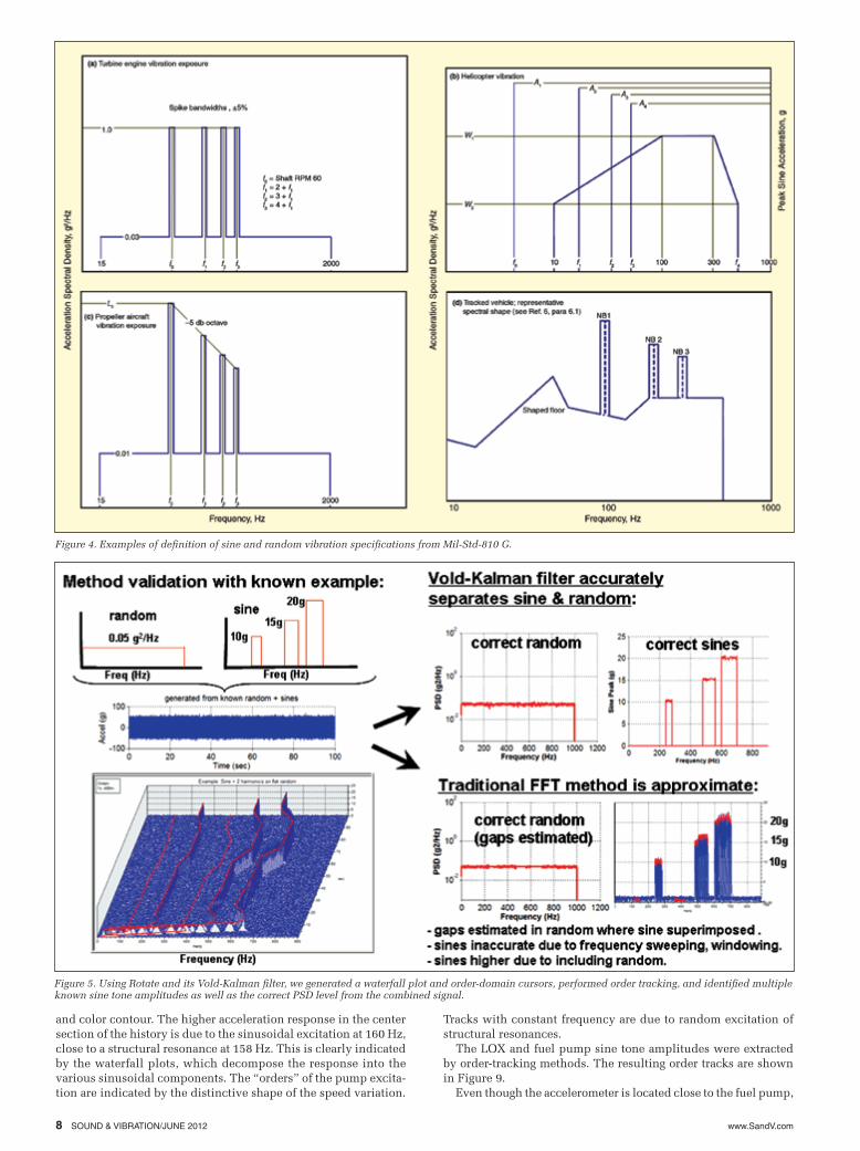
As the first part of the task of demonstrating the process of separating sine and random, known sine and random components were added in the time domain to obtain an example measurement signal. This measurement was then analyzed to separate out the sine and random components to validate the proposed sine and random separation methods. The overall process and results are shown in Figure 5. Sine tones of known amplitudes were defined in the frequency domain and then converted to the time domain by including a variation in frequency as designated by the width of the sine tone shown in the frequency domain. Each sine tone is related to the others as orders or multiples of the frequencies. A separate time function was generated for each of the three tones shown. These time functions are added to obtain the total time domain sine signal. The random component was defined as a PSD. This PSD was converted to an equivalent time signal with exactly the defined PSD. The sine was then added to the random to provide an acceleration time history for signal processing to test the ability to extract the sine and random components. In this case, NX I-deas was used to generate the time domain signals from the frequency domain definition of the sine tones and random spectrum. This signal generation uses similar algorithms to those used for control-ling shake tables to move in time in response to sine or random specifications in the frequency domain as described by Tom Irvine in his vibration data web site.3

The overall process uses order tracking and the speed change in the fundamental sine tone to recognize modes and rotating sine sources. In performing the processing to separate sine and random components from the acceleration history, the ATA Rotate™ pro-gram4 is used to do order tracking and to apply the Vold-Kalman filter5,6 to accurately identify the amplitudes, phases, and time histories of the sine tones. The use of the speed profiles, which for real data might come from the tachometer signal, is the key to achieving accurate filtering, order tracking, and order normaliza-tion with Rotate. When there is no tachometer, you may be able to

Separation of Sine and Random Com ponents from Vibration MeasurementsCharlie Engelhardt, Mary Baker, Andy Mouron, and Håvard Vold, ATA Engineering, Inc., San Diego, California

Based on a paper presented at IMAC-XXX, the 30th Conference & Exposition on Structural Dynamics, Jacksonville, FL, January/February 2012.

www.SandV.com SOUND & VIBRATION/JUNE 2012 7

generate the speed profile in other ways:• An accelerometer located close to a rotating excitation source• A track on the waterfall of the fundamental sine tone

As shown in Figure 5, we were able to generate a waterfall with order cursors that indicated which sine tones were harmonics. With the Vold-Kalman filter, we extracted from the original history the accurate sine tone histories, one history for each sine tone. We subtracted the sine tone histories from the original measurement, leaving us with an accurate history of the broadband random environment, from which we generated a PSD. The resulting separate sine and random environments very closely match the known inputs.

We also processed the data using more traditional fast-Fourier-

transform (FFT) methods. Using this alternative approach, the random and sine results are each distorted by the presence of the other. The sine tone amplitudes show errors where incremental amplitude (shown in red) from some of the random shows up as sine amplitude; the random signal has gaps associated with the frequency range where there is a sine tone missing data after subtraction of the Fourier components. It is common in making sine and random measurements to overestimate both the sine and random by allowing each to contribute to the estimate of the other.

In the next section, the processing example includes multiple-source excitations driving a structure response with electrical noise; this example is closer to a real environmental definition.

Separation from Noise and Structural ResponseA finite-element model of a simplified rocket engine was used

for a more realistic test case. This rocket engine model, shown in Figure 6, included a liquid oxygen (LOX) turbopump and a fuel turbopump that were used as source excitation locations along with the combustion chamber located at the throat above the nozzle. An accelerometer placed near the fuel turbopump is used to generate the measurement. The goal of this example is to separate the sine and random environments from this sample measurement. These accurate environments may be used to identify source functions for use as excitation for analysis.7

In this case, the challenge for data extraction is that the accel-eration response histories will not only include sine and random components but also structural dynamic responses that are not part of the source function. It is important to define the excitation specification by recognizing and separating sine tones and random excitations from combustion chamber and turbopumps and to not include in the source definition any structural resonant response or noise. Any uncertainty in the source functions’ measurements or specifications should be actual variability of the sources, not double accounting for elements of the environment.

Using this finite-element model, known fuel and LOX force sine tones and combustion chamber random forcing functions were applied as time histories at locations shown above, including small shaft speed variations in the sine tones. For this analytical example, the LOX pump force excitation was used as the tachom-eter signal. This tachometer (Figure 7, top) was processed using a threshold-crossing algorithm to generate a smooth speed profile (Figure 7, bottom). The speed profile shown in Figure 7 indicates that the pump speed ramps up and down as the rocket engine thrust is throttled. The pump speed crosses the frequencies of two significant structural modes in this example.

The resulting acceleration response near the fuel pump is shown in Figure 8; after the simulation, 60-cycle noise was added to the acceleration history. A waterfall was computed from this accelera-tion history, also shown in Figure 8 in two different formats: 3D

Figure 1. Typical environments that have mixed sine and random elements include helicopters and rocket motors.

Figure 2. Overall process of collection of environmental data and perfor-mance of separate analyses.

0 200 400 600 800 1000 1200 1400 1600Frequency, Hz

0.0001

0.001

0.01

0.1

1

PS

D G

2/H

z

Figure 3. Sine and random specification estimation from processing of combined acceleration data.

www.SandV.com8 SOUND & VIBRATION/JUNE 2012

and color contour. The higher acceleration response in the center section of the history is due to the sinusoidal excitation at 160 Hz, close to a structural resonance at 158 Hz. This is clearly indicated by the waterfall plots, which decompose the response into the various sinusoidal components. The “orders” of the pump excita-tion are indicated by the distinctive shape of the speed variation.

Figure 4. Examples of definition of sine and random vibration specifications from Mil-Std-810 G.

Figure 5. Using Rotate and its Vold-Kalman filter, we generated a waterfall plot and order-domain cursors, performed order tracking, and identified multiple known sine tone amplitudes as well as the correct PSD level from the combined signal.

Tracks with constant frequency are due to random excitation of structural resonances.

The LOX and fuel pump sine tone amplitudes were extracted by order-tracking methods. The resulting order tracks are shown in Figure 9.

Even though the accelerometer is located close to the fuel pump,

www.SandV.com SOUND & VIBRATION/JUNE 2012 9

Figure 6. The measurement challenge is to determine appropriate source functions due to excitation of turbopump sine and combustion chamber random from an accelerometer located near one of the pumps.

Figure 7. The LOX pump tachometer (top) is used to generate a speed profile (bottom).

structural resonances near the LOX pump excitation cause the ac-celeration to increase dramatically when the LOX pump crosses those resonances and dwells at 160 Hz near the second resonance.

An order track is the history of the sinusoidal amplitude, follow-ing the particular “order” of the excitation. The ridge on a waterfall may be an order if it follows the excitation speed. Order-tracking algorithms extract such ridges to produce an order track, as shown in Figure 10.

The Vold-Kalman filter is key to determining the amplitude associated only with the sine tone that follows a particular order of the speed profile. The orders of the LOX pump and fuel pump were extracted from the signal identifying these source functions, as shown in Figure 11 and Figure 12.

After each of the sine tone source contributions to the accelera-

tion response and the 60-cycle noise were identified, they were all subtracted from the original acceleration measurement. This leaves the response to the random source, as shown in Figure 13.

The structural response due to the random excitation (after removing the responses due to the sinusoidal excitations) can be seen also in Figure 14 as two ridges indicating frequencies, which do not vary with the changes in speed of the shaft over time. The frequencies of these ridges are at 149 Hz and 158 Hz, which indicate the presence of significant structural modes.

Examining the model shows that indeed there are modes at these frequencies, with participation at the source and response locations pictured in Figure 15. These two modes account for the dynamic amplification of response due to just the sine components of the excitations visible in Figures 9 and 10 and the dynamic amplifica-tion due to just the random source visible in Figure 13.

Depending on the application of interest, the separate sine and random environments defined in this way could be used directly as environments for these locations. If what is needed is an environ-ment for equipment mounted at the location of the accelerometer, then the separate sine and random environments identified above are the correct specification for the dynamic environment for that equipment. As long as the equipment or its mass is present when the measurement or simulation is performed, these separate sine and random functions provide accurate and not overly conservative environments for performing sine and random tests and analyses.

If the real interest is force excitations at different locations, such as the center of the combustion chamber and the center of gravity of each pump, then an additional step is necessary. If the source force histories are needed to analytically simulate the dynamic excitation due to the pumps and combustion chamber to assess the structural integrity of the engine, then we need to use the structural model to remove the dynamic structural transfer func-tion so we can determine an appropriate source forcing function. In our example, this transfer function can be easily obtained from the finite-element model, and the random and sine acceleration response functions shown above can be transformed to the source excitation functions.

In the real measurement situation, however, the finite-element model only approximates the dynamic transfer functions. So the use of these approximate transfer functions to back-calculate the

www.SandV.com10 SOUND & VIBRATION/JUNE 2012

Figure 8. Acceleration history (left) with corresponding 3D waterfall (center) and color contour waterfall (right).

Figure 9 Order tracks for the first two LOX pump orders (left) and first two fuel pump orders (right).

Figure 10. Comparing the LOX pump first-order track with the waterfall plots confirms that order-tracking profiles are accurate.

Figure 11. Vold-Kalman filter used for extracting orders from accelerometer history is shown here for the LOX pump source.

Figure 12. Vold-Kalman filter used for extracting orders from accelerometer history, shown here for the fuel pump source.

Figure 13. Waterfalls are shown before and after subtracting four order his-tories and electrical noise from accelerometer history leaving a definition of the random background.

excitations may create incorrect excitations (compared to actual excitations). Some type of optimization may be needed to create physically reasonable source excitations, because the actual reso-nances may not exactly match the finite-element model modes. Furthermore, the measurements may not have included the correla-tion between accelerations at different locations. In this case, the

transformation from acceleration measurements requires not only the separation of sine and random but also optimization to obtain the best fit of the response measurements with estimated source functions. This additional process is provided in Reference 7.

Conclusions and RecommendationsStructures may be overtested or analyzed with overly conserva-

tive excitations due to the measurement of environments with sine and random components incorrectly combined as well as structural responses and noise incorrectly interpreted as excitations. The sine components and the random components may be doubly accounted for as part of both the sine and random excitations. Environments defined from envelopes of this type of data may lead to attempts to drive structures at their anti-resonances or to input significantly more energy into the test article than is actually present in the

www.SandV.com SOUND & VIBRATION/JUNE 2012 11

References1. MIL-STD-810G, “Environmental Engineering Considerations & Laboratory

Tests,” October 31, 2008.2. Baker, M., Mouron, Andy, and Engelhardt, Charlie, “Combined Sine and

Random Analysis Process,” Presented at Spacecraft and Launch Vehicle Dynamic Environments Workshop, El Segundo, CA, June 7-9 2011.

3. Irvine, Tom. http://www.vibrationdata.com/NESC_Units.htm4. http://www.ata-e.com/software/rotate5. Vold, H., Mains, M., and Blough, J., “The Mathematical Background of the

Vold-Kalman Harmonic Tracking Filter,” SAE Paper No. 972007, 1997.6. Gade, S., Herlufsen, H., Konstantin-Hansen, H., Vold, H., “Characteristics

of the Vold-Kalman Order Tracking Filter,” B&K Technical Review No. 1, 1999.

7. Blelloch, P., “Matching Random Response,” Presented at Spacecraft and Launch Vehicle Dynamic Environments Workshop, El Segundo, CA, June 11, 2009.

Figure 15. Modes that have participation at source function locations of the turbopumps and combustion chamber as well as response accelerometer location.

Figure 14. Background random environment shows modal responses from structure.

The author may be reached at: charlie.engelhardt@ata-e.com.

actual environment.Using the Vold-Kalman filter with order tracking, these different

components can be accurately separated; this avoids contributing incremental amplitude from each component to the others. When accurate components are specified, the uncertainty due to actual variability in sine frequencies or statistical variations in the random sources can be properly tracked so that the final test or analysis can be assigned an accurate life or margin with known uncertainties.

This whole process requires three parts. The first part is to ac-curately separate the sine and random environments from each other and from noise. Accurate sine and random environments enable the next step: to analyze/test to the distinct sine and random environments, or analyze/test to a combined environment that includes phase and cycle definition. This analysis approach was addressed previously.2 The third part of the analysis process is to use the structural dynamic transfer functions to back out source ex-citations so that these excitations can be applied at locations other than the acceleration measurements. An approach for doing this for the random measurements has also been treated previously.7