Separation and Recovery of a Complexing Agent in the ...

Separation and Recovery of a Complexing Agent in the

Production of Lithium Hexfluorophosphate

by

Nadine Moodley

BSc. Eng.

Submitted in fulfilment of the academic requirements of

Master of Science

in

Chemical Engineering

College of Agriculture, Engineering and Science

University of KwaZulu-Natal

February 2019

Supervisors: Prof D Ramjugernath, Prof P Naidoo, Dr WM Nelson

and Dr K Wagener

2019/03/06

07/03/2019

07/03/2019

iii

ACKNOWLEDGMENTS

I would like to acknowledge and thank the following people:

The DST/NRF South African Research Chairs Initiative (SARChI), the Nuclear Energy

Corporation of South Africa (NECSA) and the Thermodynamics Research Unit (TRU) for

the support of this research.

Dr Kobus Wagener for granting permission to present the information and flow sheets

regarding the PF5 production process.

My supervisors Prof Deresh Ramjugernath, Prof Prathieka Naidoo and Dr Wayne Michael

Nelson for their guidance and for imparting their extensive knowledge.

My colleagues and research staff in the Thermodynamics Research Unit and the department:

Ayanda Khanyile, Sivanna Naicker, Sanjay Deeraj and Sikhumbuzo Sithole for their

assistance with the lab equipment and procedures.

My parents, grandparents and friends for their constant prayers, motivation and support.

And God for providing me with the strength, motivation and determination to persevere.

iv

ABSTRACT

A novel process for the production of lithium hexafluorophosphate (LiPF6) has been developed

by NECSA (Nuclear Energy Corporation of South Africa). The starting materials include

hexafluorophosphoric acid (HPF6) aqueous solution and a complexing agent, pyridine. This study

focused on the separation and recovery of the waste material from this production process

(pyridine, ethanol, water and nitrogen), with high recovery rates and final mole purities for each

component such that they can be recycled and reused in the process. Two separation schemes

were investigated. Process A treats the waste stream firstly via a flash vessel to remove the

nitrogen, then a conventional distillation column to separate the pyridine from the mixture

followed by an extractive distillation column to separate the ethanol from water. The solvent

chosen for extractive distillation was ethylene glycol. Process B follows the same scheme as

process A for the nitrogen and pyridine separation; however it uses a pervaporation membrane

modular setup, incorporating a polyvinylalcohol membrane in a spiral wound configuration, to

separate ethanol from water as opposed to the use of the extractive distillation column in process

A. Modifications were made to each process where an additional flash vessel was used to further

purify the nitrogen stream. The Aspen Plus® process simulator was used to design the proposed

separation schemes. The design and development of separation processes rely on accurate vapour

liquid equilibrium (VLE) data. The ethanol/pyridine (40 kPa, 100 kPa, 313.15 K) and

water/pyridine (40 kPa, 333.15 K) phase data were measured since the VLE data found in

literature for these systems were inconsistent. A modified recirculating VLE still was used to

measure the phase equilibrium data with sample analysis performed using a Shimadzu GC-2014.

The measured data was regressed using various thermodynamic models in Aspen Plus®. The

model that best suited the components of interest was the Peng-Robinson equation of state

incorporating the Mathias Copeman alpha function with the Wong-Sandler mixing rules and the

NRTL activity coefficient model (PR-MC-WS-NRTL). The binary parameters obtained with the

use of this model was then incorporated into the Aspen Plus® computer software where it was

used to simulate the proposed process schemes. The purpose of this is to provide a more accurate

representation of the industrial process. A sensitivity analysis on the proposed process schemes

was performed in order to obtain the optimal solution. The economic analysis showed that while

process A met the specified purity and recovery of 99.9 mol %, it had a high total annual cost

(approximately R46 million) due to the large amount of solvent required for extractive distillation.

Process B had a significantly lower total annual cost (approximately R32 million). However, this

is due to the area restriction imposed on the membrane (960 m2) due to the pyridine loss and slow

separation process as the water composition decreased. The ethanol-rich stream (retentate)

leaving the membrane unit contained a water content of 0.21 mol %; had this stream been

v

dehydrated to a water content of 0.01 mol % (similar to the purity obtained with extractive

distillation), the total membrane area would have increased to a value of 2000 m2. The area

required for the membrane then becomes practically and economically unfeasible. Furthermore,

increasing the membrane area, increases the flow rate of the recycle stream (permeate) thereby

decreasing the allowable recovery and purity of the core component, pyridine. Thus, process B

does not meet the purity and recovery specifications for pyridine and ethanol. If it is attempted to

achieve the ethanol purity specification, the membrane process becomes impractical due to the

large membrane area required and the recovery and purity of the core component pyridine

decreases. Furthermore, the additional flash vessel used in this process significantly increases the

total annual cost (R4 million) and does not improve the product purities. Process A meets the

required purity and recovery specifications for all components and is practically feasible. The

additional flash vessel used in this process recovers a further 6.18 kg/hr of ethanol whilst slightly

increasing the total annual cost (R0.14 million) and hence is the optimal solution.

vi

TABLE OF CONTENTS

Page

Preface ............................................................................................................................................ i

Declaration: Plagiarism ................................................................................................................. ii

Acknowledgements ...................................................................................................................... iii

Abstract ........................................................................................................................................ iv

Table of Contents ......................................................................................................................... vi

List of Tables ............................................................................................................................... ix

List of Figures ............................................................................................................................ xiii

Nomenclature ........................................................................................................................... xviii

Chapter 1: Introduction ..................................................................................................................1

1.1 Project Background ...............................................................................................................2

1.2 Thesis Outline .....................................................................................................................12

Chapter 2: Theoretical Background .............................................................................................13

2.1 Phase Equilibrium Data Available in Literature .................................................................14

2.2 Residue Curve Map ............................................................................................................18

2.3 Extractive Distillation .........................................................................................................21

2.4 Pervaporation ......................................................................................................................22

2.4.1 Selection of Membrane (Pervaporation) Material ...................................................... 23

2.4.2 Membrane Design ...................................................................................................... 23

2.4.3 Selection of Membrane (Pervaporation) Module ....................................................... 24

Chapter 3: Theoretical Modelling ................................................................................................27

3.1 Analyses of VLE Data ........................................................................................................27

3.2 Thermodynamic Models used in this study ........................................................................28

3.2.1 Peng-Robinson Cubic Equation of State .................................................................... 29

3.2.2 Mathias Copeman Alpha Function ............................................................................. 30

3.2.3 Mixing rules: Wong-Sandler ...................................................................................... 30

3.2.4 Activity Coefficient Models ....................................................................................... 32

3.3 Vapour Liquid Equilibrium Prediction ...............................................................................35

3.3.1 Predictive Soave Redlich Kwong (PSRK) ................................................................. 35

3.4 Data Regression ..................................................................................................................36

Chapter 4: Experimental Equipment and Procedure ....................................................................37

4.1 Low Pressure VLE Equipment ...........................................................................................37

vii

4.2 Experimental Method .........................................................................................................40

4.2.1 Preparation ................................................................................................................. 40

4.2.2 Temperature and Pressure Calibration ....................................................................... 40

4.2.3 Gas Chromatograph Thermal Conductivity Detector Calibration ............................. 43

4.2.4 Isobaric Operation ...................................................................................................... 44

4.2.5 Isothermal Operation .................................................................................................. 45

Chapter 5: Results and Discussion: Experimental VLE Data and Modelling ..............................46

5.1 Chemical Characterisation ..................................................................................................46

5.2 Vapour Pressure Measurement ...........................................................................................47

5.3 Phase Equilibrium Measurements and Modelling ..............................................................51

5.3.1 Test System: Ethanol (1) + Cyclohexane (4) ............................................................. 53

5.3.2 New Binary Phase Equilibrium Data ......................................................................... 55

5.4 Comparison of Model Parameters ......................................................................................81

Chapter 6: Process Design and Costing .......................................................................................85

6.1 Design Methodology ...........................................................................................................85

Process A ............................................................................................................................. 89

Process B ............................................................................................................................. 92

6.2 Process Optimisation ..........................................................................................................93

6.2.1 Flash Vessels .............................................................................................................. 93

6.3.2 Distillation Columns .................................................................................................. 95

Conventional Distillation Column (C-01) ........................................................................... 96

Extractive Distillation Column (C-02) ................................................................................ 99

Solvent Recovery Distillation Column (C-03) .................................................................. 101

6.3 Membrane Design .............................................................................................................102

6.4 Simulation Results ............................................................................................................105

6.5 Comparison of the Design Proposed by NECSA and this study ......................................109

6.6 Cost Evaluation .................................................................................................................110

Chapter 7: Conclusion ................................................................................................................116

Chapter 8: Recommendations ....................................................................................................119

References ..................................................................................................................................120

Appendix A: Membrane Design ................................................................................................126

Appendix B: Detailed Costing Procedure ..................................................................................129

B.1: Capital Investment Cost of Membrane and Module .......................................................129

viii

B.2: Operating Costs ...............................................................................................................129

B.3: Inter-stage Heat Exchangers ...........................................................................................131

Appendix C: Gas Chromatograph Calication Charts .................................................................132

C.1 Test System: Ethanol (1) + Cyclohexane (4) System ......................................................132

C.2 Ethanol (1) + Pyridine (3) System ...................................................................................134

C.3 Water (2) + Pyridine (3) System ......................................................................................136

Appendix D: Experimental Uncertainty Calculation .................................................................138

D.1 Temperature and Pressure Uncertainty ............................................................................139

D.2 Phase Composition Uncertainty .......................................................................................139

Appendix E: Sensitivity Analysis Plots .....................................................................................141

E.1 Process 1FE (1 flash, extractive distillation): ...................................................................141

Solvent Recovery Column (C-03) ..................................................................................... 141

E.2 Process 2FE (2 flash, extractive distillation): ...................................................................142

Conventional Distillation Column (C-01) ......................................................................... 142

Extractive Distillation Column (C-02) .............................................................................. 143

Solvent Recovery Column (C-03) ..................................................................................... 145

E.3 Process 1FM (1 flash, membranes) ..................................................................................146


E.4 Process 2FM (2 flash, membranes) ..................................................................................147


ix

LIST OF TABLES

Table 1.1: Stream results for the PF5 production process proposed by NECSA ........................... 5

Table 1.2: Stream results for the waste treatment process proposed by NECSA ....................... 10

Table 2.1: Boiling points and azeotropic compositions for the system ethanol (1) + water (2) +

pyridine (3) generated on Aspen Plus® at 80 kPa. ..................................................................... 18

Table 3.1: Significance of 𝑘𝑖𝑗 binary interaction parameter ....................................................... 31

Table 3.2: Suitable guideline for 𝛼𝑖𝑗 parameter .......................................................................... 34

Table 4.1: Operating conditions for the Shimadzu GC- 2014 ..................................................... 43

Table 5.1: Chemical characterisation at 293.15 K ...................................................................... 46

Table 5.2: Combined expanded uncertainties for temperature and pressure............................... 47

Table 5.3: Comparison of experimental vapour pressure data for cyclohexane to literature sources

..................................................................................................................................................... 48

Table 5.4: Comparison of the experimental vapour pressure data for ethanol to literature sources.

..................................................................................................................................................... 49

Table 5.5: Comparison of the experimental vapour pressure data for pyridine to literature sources.

..................................................................................................................................................... 50

Table 5.6: Average absolute deviation (AAD) and average absolute relative deviation (AARD)

for the experimental vapour pressures using the reference sources. ........................................... 51

Table 5.7: Uncertainties observed in temperature and pressure for the systems of interest ....... 51

Table 5.8: Uncertainties observed in composition for the systems of interest ............................ 52

Table 5.9: Combined expanded uncertainties for temperature, pressure and mole compositions for

the VLE binary systems, averaged over all data points for each system .................................... 52

Table 5.10: Regressed MC parameters (PR-MC-EoS) ............................................................... 55

Table 5.11: Deviations in the experimental vapour pressure data from modelled data using the PR

EoS with the MC alpha function ................................................................................................. 56

x

Table 5.12: Comparison of the experimental VLE data to modelled data for the isobaric ethanol

(1) + pyridine (3) system at 40 kPa ............................................................................................. 65

Table 5.13: Comparison of the experimental VLE data to modelled data for the ethanol (1) +

pyridine (3) system at 100 kPa .................................................................................................... 66

Table 5.14: Comparison of the experimental VLE data to modelled data for the ethanol (1) +

pyridine (3) system at 313.15 K. ................................................................................................. 67

Table 5.15: Data regression deviations for the isobaric ethanol (1) + pyridine (3) binary system.

..................................................................................................................................................... 68

Table 5.16: Data regression deviations for the isothermal ethanol (1) + pyridine (3) binary system.

..................................................................................................................................................... 69

Table 5.17: Model parameters regressed for the ethanol (1) + pyridine (3) binary system ........ 69

Table 5.18: Azeotropic data for the water (2) + pyridine (3) system .......................................... 75

Table 5.19: Comparison of the experimental VLE data to modelled data for the water (2) +

pyridine (3) system at 40 kPa ...................................................................................................... 76

Table 5.20: Comparison of the experimental VLE data to modelled data for the water (2) +

pyridine (3) system at 333.15 K .................................................................................................. 77

Table 5.21: Data regression deviations for the isobaric water (2) + pyridine (3) binary system 78

Table 5.22: Data regression deviations for the isothermal water (2) + pyridine (3) binary system.

..................................................................................................................................................... 79

Table 5.23: Model parameters regressed for the water (2) + pyridine (3) binary system ........... 80

Table 5.24: Data regression deviations for the systems studied averaged over all points. ......... 84

Table 6.1: Stream results for process 1FE (1-flash extractive) ................................................... 87

Table 6.2: Stream results for process 2FE (2-flash extractive) ................................................... 88

Table 6.3: Stream results for process 1FM (1-flash membrane) ................................................. 91

Table 6.4: Stream results for process 2FM (2-flash membrane) ................................................. 91

Table 6.5: Component Murphree Efficiencies ............................................................................ 95

xi

Table 6.6: Critical properties of components .............................................................................. 96

Table 6.7: Variation of feed stage (FS) location and reflux ratio (RR) to meet desired distillate

specifications for column C-01 (process A: 1 flash extractive) .................................................. 97

Table 6.8: Extractive distillation column specifications for each case for column C-02 (process

A: 1 flash extractive) ................................................................................................................. 100

Table 6.9: Membrane and module specifications...................................................................... 103

Table 6.10: First row results of module configuration .............................................................. 104

Table 6.11: Distillation column specifications for process A (2FE & 1FE) ............................. 105

Table 6.12: Distillation column specifications for process B (2FM & 1FM) ........................... 105

Table 6.13: Flash vessel specifications ..................................................................................... 106

Table 6.14: Final stream compositions and purities for process A: .......................................... 107

Table 6.15: Final stream compositions and purities for process B ........................................... 109

Table 6.16: Capital and operating cost summary ...................................................................... 111

Table 6.17: Purity and flow rate of relevant streams ................................................................ 114

Table A.1: Coefficients for the Antoine equation: .................................................................... 128

Table A.2: Coefficients for the Van Laar equation: .................................................................. 128

Table B.1: Literature cost of membrane and module ................................................................ 129

Table B.2: Utility costs ............................................................................................................. 129

Table B.3: Conversion of currencies to rands ........................................................................... 130

Table B.4: Chemical Engineering Plant Cost Index ................................................................. 130

Table B.5: Enthalpy of vaporisation and heat capacities .......................................................... 131

Table B.6: Enthalpy of vaporisation and heat capacities from Aspen Plus® ........................... 131

Table E.1: Variation of feed stage location with reflux ratio .................................................... 141


xii

Table E.3: Extractive distillation column specifications for each case ..................................... 144




xiii

LIST OF FIGURES

Figure 1.1: PF5 production process as proposed by NECSA ........................................................ 4

Figure 1.2: Waste treatment process as proposed by NECSA ...................................................... 9

Figure 2.1: Literature data available for ethanol (1) + pyridine (3) system ................................ 16

Figure 2.2: Some of the literature data available for the water (2) + pyridine (3) system ......... 17

Figure 2.3: Residue curve map generated on Aspen Plus® using the NRTL activity coefficient

model with azeotropes (mole fractions) at 80 kPa ...................................................................... 19


model with stream compositions and azeotropes (mole fractions) at 80 kPa ............................ 20

Figure 2.5: Schematic of the pervaporation process ................................................................... 23

Figure 4.1: Schematic diagram of the VLE recirculating still .................................................... 38

Figure 4.2: Temperature calibration for the VLE still ................................................................ 41

Figure 4.3: Uncertainty in temperature calibration for the VLE still .......................................... 42

Figure 4.4: Pressure calibration for the VLE still ....................................................................... 42

Figure 4.5: Uncertainty in pressure calibration for the VLE still ................................................ 43

Figure 5.1: Vapour pressure data for cyclohexane.. .................................................................... 48

Figure 5.2: Vapour pressure data for ethanol. ............................................................................. 49

Figure 5.3: Vapour pressure data for pyridine. ........................................................................... 50

Figure 5.4: Isobaric VLE data for the ethanol (1) + cyclohexane (4) system at 40 kPa. ............ 53

Figure 5.5: Isobaric x-y data for the ethanol (1) + cyclohexane (4) system at 40 kPa. ............... 53

Figure 5.6: Isothermal VLE data for the ethanol (1) + cyclohexane (4) system at 313.15 K.. ... 54

Figure 5.7: Isothermal x-y data for the ethanol (1) + cyclohexane (4) system at 313.15 K. ....... 54

Figure 5.8: Isobaric VLE data for the ethanol (1) + pyridine (3) system at 40 kPa. Comparison of

experimental data to literature and predicted data ...................................................................... 56

xiv

Figure 5.9: Isobaric x-y data for the ethanol (1) + pyridine (3) system at 40 kPa. Comparison of


Figure 5.10: Isobaric VLE data for the ethanol (1) + pyridine (3) system at 100 kPa. Comparison

of experimental data to literature and predicted data .................................................................. 57

Figure 5.11: Isobaric x-y data for the ethanol (1) + pyridine (3) system at 100 kPa. Comparison


Figure 5.12: Isothermal VLE data for the ethanol (1) + pyridine (3) system at 313.15 K.

Comparison of experimental data to literature and predicted data .............................................. 59

Figure 5.13: Isothermal x-y data for the ethanol (1) + pyridine (3) system at 313.15 K. Comparison

of experimental data to literature and predicted data. ................................................................. 59


of experimental data to modelled data ........................................................................................ 60

Figure 5.15: Isobaric x-y data for the ethanol (1) + pyridine (3) system at 40 kPa. Comparison of

experimental data to modelled data ............................................................................................. 61



Figure 5.17: Isobaric x-y data for the ethanol (1) + pyridine (3) system at 100 kPa. Comparison


Figure 5.18: Isothermal VLE data for the ethanol (1) + pyridine (3) system at 313.15 K.

Comparison of experimental data to modelled data .................................................................... 63

Figure 5.19: Isothermal x-y data for the ethanol (1) + pyridine (3) system at 313.15 K. Comparison


Figure 5.20: Isobaric VLE data for the water (2) + pyridine (3) system at 40 kPa. Comparison of


Figure 5.21: Isobaric x-y data for the water (2) + pyridine (3) system at 40 kPa. Comparison of


Figure 5.22: Isothermal VLE data for the water (2) + pyridine (3) system at 333.15 K. Comparison


xv

Figure 5.23: Isothermal x-y data for the water (2) + pyridine (3) system at 333.15 K. Comparison


Figure 5.24: Isobaric VLE data for the water (2) + pyridine (3) system at 40 kPa. Comparison of

experimental data to modelled data. ............................................................................................ 72

Figure 5.25: Isobaric x-y data for the water (2) + pyridine (3) system at 40 kPa. Comparison of

experimental data to modelled data. ............................................................................................ 73

Figure 5.26: Isothermal VLE data for the water (2) + pyridine (3) system at 333.15 K. Comparison


Figure 5.27: Isothermal x-y data for the water (2) + pyridine (3) system at 333.15 K Comparison


Figure 5.28: Isothermal VLE data for the ethanol (1) + pyridine (3) system. Comparison of

literature data to modelled data using the Dortmund Data Bank and Aspen Plus® ................... 81

Figure 5.29: Isothermal VLE data for the water (2) + pyridine (3) system. Comparison of literature

data to modelled data using the Dortmund Data Bank and Aspen Plus®. .................................. 82

Figure 5.30: Isothermal x-y data for the water (2) + pyridine (3) system. Comparison of literature

data to modelled data using the Dortmund Data Bank and Aspen Plus®. .................................. 83

Figure 6.1: Process A .................................................................................................................. 86

Figure 6.2: Process B .................................................................................................................. 90

Figure 6.3: Influence of pressure on the nitrogen mole purity, nitrogen recovery and ethanol mass

flow rate in the vapour outlet for F-01 (1-flash process) ............................................................ 93





Figure 6.6: Influence of the number of stages on TAC for column C-01, process A: 1 flash

extractive ..................................................................................................................................... 98

Figure 6.7: Influence of the feed stage on the total annual cost at 75 stages for column C-01,

process A: 1 flash extractive ....................................................................................................... 98

xvi

Figure 6.8: Influence of number of stages on reboiler heat duty for column C-02, process A: 1

flash extractive ............................................................................................................................ 99

Figure 6.9: Effect of solvent to feed ratio on RHD for case 5 for column C-02, process A: 1 flash

extractive ................................................................................................................................... 100

Figure 6.10: Total annual cost for the different cases in column C-02, process A, 1 flash extractive.

................................................................................................................................................... 101

Figure A.1: Permeation flux of ethanol as a function of ethanol feed concentration ................ 127

Figure A.2: Permeation flux of water as a function of ethanol feed concentration................... 128

Figure C.1: GC calibration for the ethanol (1) + cyclohexane (4) system in the more dilute regions

of ethanol. Representation of the relationship between the number of moles vs the peak area. 132

Figure C.2: GC calibration for ethanol (1) + cyclohexane (4) system in the more dilute regions of

ethanol. Deviations in composition using a second order polynomial. ..................................... 132

Figure C.3: GC calibration for the ethanol (1) + cyclohexane (4) system in the more concentrated

regions of ethanol. Representation of the relationship between the number of moles vs the peak

area. ........................................................................................................................................... 133

Figure C.4: GC calibration for the ethanol (1) + cyclohexane (4) system in the more concentrated

regions of ethanol. Deviations in composition using a second order polynomial. .................... 133

Figure C.5: GC calibration for the ethanol (1) + pyridine (3) system in the more dilute regions of

ethanol. Representation of the relationship between the number of moles vs the peak area. ... 134

Figure C.6: GC calibration for the ethanol (1) + pyridine (3) system in the more dilute regions of

ethanol. Deviations in composition using a second order polynomial ...................................... 134

Figure C.7: GC calibration for the ethanol (1) + pyridine (3) system in the more concentrated


area. ........................................................................................................................................... 135


regions of ethanol. Deviations in composition using a second order polynomial ..................... 135

Figure C.9: GC calibration for the water (2) + pyridine (3) system in the more dilute regions of

water. Representation of the relationship between the number of moles vs the peak area. ...... 136

xvii


water. Deviations in composition using a second order polynomial. ........................................ 136

Figure C.11: GC calibration for the water (2) + pyridine (3) system in the more concentrated

regions of water. Representation of the relationship between the number of moles vs the peak

area. ........................................................................................................................................... 137


regions of water. Deviations in composition using a second order polynomial. ....................... 137

Figure E.1: Influence of number of stages on the total annual cost .......................................... 141

Figure E.2: Influence of feed entry stage on the total annual cost at 32 stages ........................ 141


Figure E.4: Influence of feed entry stage on total annual cost at 73 stages .............................. 142

Figure E.5: Influence of number of stages on reboiler heat duty .............................................. 143

Figure E.6: Influence of solvent to feed ratio on reboiler heat duty for case 6 ......................... 143

Figure E.7: Total annual cost for the different cases in the extractive distillation column ....... 144


Figure E.9: Influence of feed entry stage on total annual cost at 33 stages .............................. 145

Figure E.10: Influence of number of stages on the total annual cost ........................................ 146

Figure E.11: Influence of feed entry stage on the total annual cost at 65 stages ...................... 146

Figure E.12: Influence of number of stages on the total annual cost ........................................ 147

Figure E.13: Influence on feed entry stage on the total annual cost at 63 stages ...................... 147

xviii

NOMENCLATURE

Symbol

a Intermolecular attraction force parameter in PR EoS

A Integrated peak area from GC (m2)

𝐴𝐸 Excess Helmholtz free energy (kJ/mol)

𝐴𝑘 Differential area of element k in membrane (m2)

𝐴12, 𝐴21 Van Laar equation constants

A, B, C Antoine equation constants

𝑎𝑖𝑗 , 𝑏𝑖𝑗 , 𝑐𝑖𝑗, 𝑑𝑖𝑗 , 𝑒𝑖𝑗, 𝑓𝑖𝑗 NTRL parameters from Aspen Plus®

b Molecular size parameter in EoS, half width interval in type B

evaluation

c Composition (kmol/h)

C Mathias Copeman parameter

𝐶𝑓 Annual fixed cost

𝐶𝑃 Heat capacity (kJ/kmol.h)

𝐶𝑉 Process variable cost

f Fugacity (kPa)

𝑓𝑐 Fixed capital investment

F Response factor from GC

𝐹𝐹 Feed flow rate to membrane (kmol/h)

𝐹𝑃 Permeate flow rate from membrane (kmol/h)

G Gas

𝐺𝐸 Excess Gibbs free energy (kJ/mol)

𝐺𝑖𝑗, 𝐺𝑗𝑖 Parameter in the NRTL model (kJ/mol)

∆ℎ𝑣𝑎𝑝 Enthalpy of vapourisation (kJ/kmol)

xix

𝑖𝑚 Minimum acceptable rate of return

𝑖𝑟 Fixed capital recovery rate

J Normalised permeation flux (kmol/m2.h.kPa)

k Coverage factor

𝑘𝑖𝑗,𝑙𝑖𝑗 Binary interaction parameter for the Wong-Sandler mixing rule

L Liquid

m Mass (kg)

n Number of moles (mol)

𝑁𝑃 Number of points

P Pressure (kPa), permeate (kmol/h)

𝑝𝑜 Vapour pressure on feed side of membrane (kPa)

𝑝" Vapour pressure on permeate side of membrane (kPa)

Q Duty (kW), permeation flux (kmol/h/m2)

𝑄𝐶 Condenser duty (kW)

𝑄𝑅 Reboiler duty (kW)

𝑄𝑡𝑜𝑡 Total permeation flux (kmol/h.m2)

R Universal gas constant (J/mol.K), retentate (kmol/h)

S Solid

T Temperature (K)

𝑇𝑅 Reduced temperature (K)

TRUE True value of the property

u Uncertainty

𝑢𝐶 Combined standard uncertainty

𝑈𝐶 Combined expanded uncertainty

V Vapour, volume (m3)

xx

𝑉𝑙 Saturated liquid molar volume (m3/mol)

𝑣 Molar volume (m3/mol) in PR EoS

w Weight fraction

x Liquid phase mole fraction

y Vapour phase mole fraction

Greek Symbols

𝛼 Scaling factor in the PR EoS, non-randomness interaction parameter

in the NRTL model

𝛼𝑖 (T) Alpha function in cubic equation of state

𝜏𝑖𝑗, 𝜏𝑗𝑖 Parameter in the NRTL model

𝛾 Activity Coefficient

𝜎 Standard deviation for type A evaluation

ф Fugacity coefficient

Φ Ratio of fugacity coefficient and Poynting correction factor

𝜔 Acentric factor

Subscript

bal Mass balance

c Critical property

calc Calculated

cali Calibrated

exp Experimental

fluct Fluctuation

i, j Component identification

ij Interaction between molecular species i and j

xxi

lit Literature

rep Repeatability

std Standard

Superscripts

sat Property evaluated at the saturation pressure

o Standard state

l Liquid

v Vapour

^ Mixture

E Excess

Abbreviations

AAD Absolute Average Deviation

AARD Absolute Average Relative Deviation

DDB Dortmund Data Bank

DSV Design/Spec Vary

EoS Equation of State

FS Feed Stage

GC Gas Chromatograph

MC Mathias Copeman

NoS Number of Stages

NIST National Institute of Standards and Technology

NRTL Non-Random-Two-Liquid

PR Peng-Robinson

PSRK Predictive-Soave-Redlich-Kwong

xxii

PVA Polyvinyl alcohol

RCM Residue Curve Map

RHD Reboiler Heat Duty

RMSE Root Mean Square Error

RR Reflux Ratio

RSS Root Sum Squares

S/F Solvent to Feed ratio

TAC Total Annual Cost

TCD Thermal Conductivity Detector

VLE Vapour Liquid Equilibrium

WS Wong-Sandler

UNIFAC Universal Functional Group Activity Coefficient Model

UNIQUAC Universal Quasi-Chemical Activity Coefficient Model

1

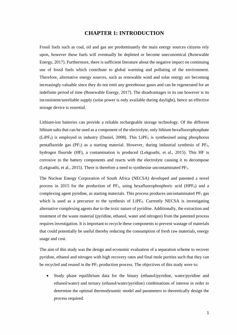
CHAPTER 1: INTRODUCTION

Fossil fuels such as coal, oil and gas are predominantly the main energy sources citizens rely

upon, however these fuels will eventually be depleted or become uneconomical (Renewable

Energy, 2017). Furthermore, there is sufficient literature about the negative impact on continuing

use of fossil fuels which contribute to global warming and polluting of the environment.

Therefore, alternative energy sources, such as renewable wind and solar energy are becoming

increasingly valuable since they do not emit any greenhouse gases and can be regenerated for an

indefinite period of time (Renewable Energy, 2017). The disadvantages in its use however is its

inconsistent/unreliable supply (solar power is only available during daylight), hence an effective

storage device is essential.

Lithium-ion batteries can provide a reliable rechargeable storage technology. Of the different

lithium salts that can be used as a component of the electrolyte, only lithium hexafluorophosphate

(LiPF6) is employed in industry (Daniel, 2008). This LiPF6 is synthesised using phosphorus

pentafluoride gas (PF5) as a starting material. However, during industrial synthesis of PF5,

hydrogen fluoride (HF), a contamination is produced (Lekgoathi, et al., 2015). This HF is

corrosive to the battery components and reacts with the electrolyte causing it to decompose

(Lekgoathi, et al., 2015). There is therefore a need to synthesise uncontaminated PF5.

The Nuclear Energy Corporation of South Africa (NECSA) developed and patented a novel

process in 2015 for the production of PF5, using hexafluorophosphoric acid (HPF6) and a

complexing agent pyridine, as starting materials. This process produces uncontaminated PF5 gas

which is used as a precursor to the synthesis of LiPF6. Currently NECSA is investigating

alternative complexing agents due to the toxic nature of pyridine. Additionally, the extraction and

treatment of the waste material (pyridine, ethanol, water and nitrogen) from the patented process

requires investigation. It is important to recycle these components to prevent wastage of materials

that could potentially be useful thereby reducing the consumption of fresh raw materials, energy

usage and cost.

The aim of this study was the design and economic evaluation of a separation scheme to recover

pyridine, ethanol and nitrogen with high recovery rates and final mole purities such that they can

be recycled and reused in the PF5 production process. The objectives of this study were to:

Study phase equilibrium data for the binary (ethanol/pyridine, water/pyridine and

ethanol/water) and ternary (ethanol/water/pyridine) combinations of interest in order to

determine the optimal thermodynamic model and parameters to theoretically design the

process required.

2

Investigate typical separation methods for the components of interest to gain an

understanding on the current processes used and to determine whether a cheaper and more

efficient alternative can be found.

Propose a separation scheme to recover and recycle pyridine, ethanol and nitrogen with

high recovery rates and final mole purities such that they can be recycled and reused in

the PF5 production process.

Process simulation tools are able to represent (based on the information and thermodynamic

models inherent in the package) the behaviour of a chemical process and are very useful to

determine the validity of the design from an energetic and economic point of view. The Aspen

Plus® process simulator was used to design the proposed separation schemes. The design and

development of separation processes rely on accurate vapour liquid equilibrium (VLE) data.

Therefore, the first step in this study was to perform VLE experiments to acquire the binary

ethanol/pyridine and water/pyridine phase data since the VLE data found in literature for these

systems were inconsistent. A modified recirculating VLE still was used to measure the phase

equilibrium data with sample analysis performed using a Shimadzu GC-2014. The isothermal and

isobaric binary VLE data measurements were undertaken for pyridine + ethanol at 313.15 K; 100

kPa and 40 kPa respectively. The isothermal and isobaric VLE data measurements for pyridine +

water was performed at 333.15 K and 40 kPa respectively. The measured data was regressed on

Aspen Plus® using various thermodynamic models to obtain the binary parameters required for

process design. With the use of these parameters, two process schemes were designed and a

sensitivity analysis performed in order to obtain the optimal solution. There-after, an economic

analysis was performed to compare the processes and determine its feasibility.

1.1 Project Background

The current industrial process for LiPF6 involves reacting PF5 and LiF (dry method) in the

presence of anhydrous hydrofluoric acid (Nakajima and Groult, 2011). The PF5 gas normally used

in this reaction is produced from fluorine gas, which is contaminated with impurities such as N2,

SF4, COF2 and HF. Contamination with HF results in the corrosion of the battery components and

consequently distillation is required to purify the PF5 gas. However, distillation is an additional

and expensive step in the process (Lekgoathi, et al., 2015). The production process as proposed

by NECSA differs from the current method in that it involves cationic exchange and emanates

from the idea of Willmann, et al. (1999) where it is believed that the direct synthesis of LiPF6 is

possible when the hydrogen ion in the pyridinium hexafluorophosphate (C5H5NHPF6) is

exchanged with the lithium ion, forming C5H5NLiPF6. According to Lekgoathi, et al. (2015), this

direct route for LiPF6 synthesis is not viable since the C5H5NLiPF6 compound is stable, hence the

separation of LiPF6 from pyridine is not possible. However, the same technique used to synthesise

3

the LiPF6–pyridine complex can be utilised to synthesise the less electronegative alkali metal

hexafluorophosphate NaPF6. This compound forms less stable complexes than the LiPF6–pyridine

complex and can therefore be used as a PF5 generator by thermal decomposition as shown in

equation 1.1.

𝑁𝑎𝑃𝐹6∆𝑇 (𝐾)↔ 𝑃𝐹5 (𝑔) + 𝑁𝑎𝐹(𝑠) (1.1)

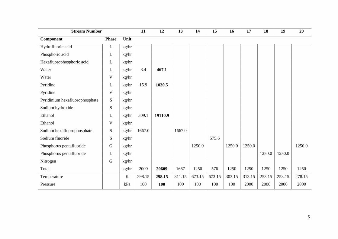
This process is illustrated in Figure 1.1. The PF5 gas produced is used as a precursor to the

synthesis of LiPF6. The stream compositions and conditions are presented in Table 1.1. The waste

streams that require purification and recycling from Figure 1.1 are streams 5 (pyridine to

pervaporation), 12 (liquid to pervaporation system) and 25 (wet N2 to gas membranes). These

streams are highlighted in red in Figure 1.1 and highlighted in bold in Table 1.1.

4

Figure 1.1: PF5 production process (NECSA, 2017)

Pyridine from

pervaporation system

Hydrofluoric acid

from storage

Phosphoric acid

from storage

Cooler

HE-01

61 W

Hexafluorophosphoric acid reactor R-01

P-01 Sodium hydroxide

Ethanol from distillation system

Sodium hydroxide

dissolution tank T-01

Sodium hydroxide

solution storage vessel tank V-01

Nitrogen from gas membranes

P-04

118 kW

P-02

Cooler

HE-02

303 kW

Pyridinium

hexafluorophosphate

reactor R-02

Sodium

hexafluorophosphate

reactor R-03

Rotary drum

filter F-01

Filter

F-01

FC-01

7.5 kW

HE-03

300 kW

Rotary dryer

D-01 Rotary kiln

K-01

7 MW

HE-04

107.4 kW

PF5

Compressor

MC-01

77 kW

PF5

Condenser

C-01

40 kW

PF5 Day

storage V-02

PF5

Compressor

MC-02

13 kW

Evaporator

HE-05

26 kW

Cooler HE-06

12 kW

Pyridine to

pervaporation

Wet nitrogen to

gas membranes

Liquid to

pervaporation system

Phosphorous pentafluoride

into cylinders

Sodium fluoride to

fluoride recovery

5

Table 1.1: Stream results for the PF5 production process proposed by NECSA

Stream Number 1 2 3 4 5 6 7 8 9 10

Component Phase Unit

Hydrofluoric acid L kg/hr 1190.8

Phosphoric acid L kg/hr 972.2

Hexafluorophosphoric acid L kg/hr 1666.7

Water L kg/hr 171.6 2.7 171.6 886.0 296.0 474.6

Water V kg/hr

Pyridine L kg/hr 1832.9 785.7 262.2 1047.2

Pyridine V kg/hr

Pyridinium hexafluorophosphate S kg/hr 2233.0

Sodium hydroxide S kg/hr 397.0 397.0

Ethanol L kg/hr 38.8 16.3 5.4 19414.6 19420.0 19420.0

Ethanol V kg/hr

Sodium hexafluorophosphate S kg/hr 1666.7

Sodium fluoride S kg/hr

Phosphorus pentafluoride G kg/hr

Phosphorus pentafluoride L kg/hr

Nitrogen G kg/hr

Total kg/hr 1191 1144 1874 1838 1688 2797 22603 397 19420 19817

Temperature K 298.15 298.15 298.15 303.15 303.15 303.15 298.15 298.15 298.15 298.15

Pressure kPa 100 100 100 100 100 100 100 100 100 100

6

Stream Number 11 12 13 14 15 16 17 18 19 20


Hydrofluoric acid L kg/hr

Phosphoric acid L kg/hr

Hexafluorophosphoric acid L kg/hr

Water L kg/hr 8.4 467.1

Water V kg/hr

Pyridine L kg/hr 15.9 1030.5

Pyridine V kg/hr

Pyridinium hexafluorophosphate S kg/hr

Sodium hydroxide S kg/hr

Ethanol L kg/hr 309.1 19110.9

Ethanol V kg/hr

Sodium hexafluorophosphate S kg/hr 1667.0 1667.0

Sodium fluoride S kg/hr 575.6

Phosphorus pentafluoride G kg/hr 1250.0 1250.0 1250.0 1250.0

Phosphorus pentafluoride L kg/hr 1250.0 1250.0

Nitrogen G kg/hr

Total kg/hr 2000 20609 1667 1250 576 1250 1250 1250 1250 1250

Temperature K 298.15 298.15 311.15 673.15 673.15 303.15 313.15 253.15 253.15 278.15

Pressure kPa 100 100 100 100 100 100 2000 2000 2000 2000

7

Stream Number 21 22 23 24 25


Hydrofluoric acid L kg/hr

Phosphoric acid L kg/hr

Hexafluorophosphoric acid L kg/hr

Water L kg/hr

Water V kg/hr 0.6 7.6

Pyridine L kg/hr

Pyridine V kg/hr 16.7

Pyridinium hexafluorophosphate S kg/hr

Sodium hydroxide S kg/hr

Ethanol L kg/hr

Ethanol V kg/hr 309.1

Sodium hexafluorophosphate S kg/hr


Phosphorus pentafluoride G kg/hr 1250.0 1250.0

Phosphorus pentafluoride L kg/hr

Nitrogen G kg/hr 9524.0 9804.0 9524.0

Total kg/hr 1250 1250 9525 9804 9857

Temperature K 313.15 303.15 298.15 313.15 313.15

Pressure kPa 2860 2860 100 100 100

8

Figure 1.2 presents the process scheme proposed by NECSA to treat waste streams 5, 12 and 25.

It is important to note that this separation scheme has not been designed but merely suggested.

Figure 1.2 comprises the following process streams:

Stream 5: Pyridine from Reactor R-02

Stream 12: Liquid from Rotary Filter

Stream 23: Nitrogen gas to dryer D-01

Stream 25: Nitrogen Gas from Rotary Drum D-01

Stream 27: Liquid from Condenser C-03

Stream 28: Feed to Gas Membrane System GM-101

Stream 29: Vapour from Gas Membrane System GM-101 (Ethanol + Pyridine)

Stream 30: Vapour from Gas Menbrane System GM-101 (Nitrogen +Water)

Stream 31: Nitrogen gas to atmosphere

Stream 32: Liquid from Pervaporation Feed Tank T-09

Stream 34: Vapour from Pervaporation System PV-101

Stream 36: Feed to Distillation System DC-101

Stream 37: Feed to Ethanol Storage Tank T-12

Stream 38: Feed to Pyridine Storage Tank T-13

Stream 25 (comprising nitrogen, ethanol, water and pyridine) is first fed to a compressor (MC-

03) to set the required temperature and pressure and there-after to a condenser (C-03) to separate

some of the ethanol, water and pyridine from nitrogen. Stream 28 from C-03 is then fed to a gas

permeation unit (GM-01) where only nitrogen and water leave in the permeate (stream 30). This

stream is sent to a temperature swing absorption dryer (AD-01) to remove the water from

nitrogen. Make-up nitrogen gas is then mixed with stream 23 from AD-01 and sent for use in the

PF5 production process. Streams 5, 12 and 27 (comprising ethanol, water and pyridine) are mixed

and sent to a pervaporation unit (PV-01) to remove the water from the mixture. Stream 34 from

PV-01 is then mixed with stream 29 from GM-01 and sent to a distillation column (DC-01) where

ethanol is obtained in stream 37 and pyridine achieved in stream 38. These streams are then sent

for use in the PF5 production process.

9

Figure 1.2: Waste treatment process (NECSA, 2017)

25 26

5

12

28

32

29

27

39

23

30

36

34

35

37

9

31

3

38

33

Nitrogen gas make-up

Pyridine from reactor R-02

Liquid from rotary filter

Nitrogen gas from rotary drier D-01

Pyridine to pyridinium

hexafluorophosphate

reactor R-02

Ethanol to NaOH dissolution tank T-01

Steam to atmosphere

Nitrogen gas to atmosphere

Nitrogen gas to dryer D-01

Condenser C-03

287 kW

Compressor

MC-03 919 kW

Pervaporation feed tank T-09

P-07

Heat

exchanger

HE-10 218 kW

Pervaporation system PV-01

Gas membrane system GM-01

Reboiler

Condenser 13.6 MW

Distillation system DC-01

Temperature swing

adsorption dryer AD-01

Pyridine storage tank T-13

Ethanol storage tank T-12

P-11

P-10

10

Table 1.2 presents the stream composition and conditions for the waste treatment process proposed by NECSA. This process was not designed but merely

suggested. The values presented in the table comprise predominantly of assumptions and estimations.

Table 1.2: Stream results for the waste treatment process proposed by NECSA

Stream Number 26 27 28 29 30 31 32 33 34 35


Water L kg/hr 6.0 1359.1

Water V kg/hr 7.6 1.5 1.5 0.9 1359.1 2.7 1356.4

Pyridine L kg/hr 10.2 1826.5

Pyridine V kg/hr 16.7 6.5 6.5 1826.5 1826.5


Ethanol V kg/hr 309.1 10.2 10.2 19409.8 19409.8


Nitrogen G kg/hr 9524.0 9524.0 9524.0 476.2

Total kg/hr 9857 315 9542 17 9526 477 22595 22595 21239 1356

Temperature K 353.15 280.15 280.15 293.15 293.15 343.15 298.15 393.15 373.15 303.15

Pressure kPa 4000 4000 4000 4000 600 100 100 100 100 500

11

Stream Number 36 37 38 39


Water L kg/hr 0 2.7

Water V kg/hr 2.7

Pyridine L kg/hr 1832.9

Pyridine V kg/hr 1832.9


Ethanol V kg/hr 19420.0


Nitrogen G kg/hr 476.2

Total kg/hr 21256 19381 1875 476

Temperature K 303.15 351.15 373.15 298.15

Pressure kPa 100 100 100 100

12

In this study, it was intended to preliminary design NECSA’s proposal presented in Figure 1.2

however, this could not be done. In order to design a membrane, experimental permeation flux

data for the system of components needs to be available. After extensive research, no data for

both the nitrogen/ethanol/water/pyridine system (fed to the gas permeation unit) and the

ethanol/water/pyridine system (fed to the pervaporation unit) were found in literature; hence the

membrane design presented in Figure 1.2 could not be performed.

Furthermore, physically measuring the permeation flux data was not in the scope of this project

since the focus of the thermodynamics research group is phase equilibrium measurements and

simulation design; hence the equipment required for measurements were not available. Therefore,

alternative separation schemes for the waste treatment process were developed and designed in

this work.

1.2 Thesis Outline

The thesis has been compiled in 8 chapters. Chapter 1 provides a brief background to the process

and presents the aims and objectives. Chapter 2 describes the separation technologies available

and the phase behaviour of the systems studied. Chapter 3 presents a brief review of the

thermodynamic principles for low pressure VLE data correlation and analysis. Chapter 4 focuses

on the description of the low pressure VLE recirculating still and the experimental procedure

followed in this study. Chapter 5 presents and analyses the experimental results via a comparison

to literature data, predicted data and modelled data. Chapter 6 describes the process design and

costing for both processes. The conclusion is presented in chapter 7 followed by the

recommendations in chapter 8.

13

CHAPTER 2: THEORETICAL BACKGROUND

This chapter describes the separation technologies available and the phase behaviour of the

systems studied. A mixture of four components (nitrogen, ethanol, water and pyridine) required

separation and recovery. Nitrogen can be easily removed with the use of a flash vessel, condenser,

etc. A typical separation method for the ethanol (1) + water (2) + pyridine (3) system is distillation.

However, there exist two homogenous binary azeotropes in this mixture, one between ethanol and

water and the other between water and pyridine. Azeotropic mixtures cannot be easily separated

by conventional distillation and hence require enhanced separation techniques. Some of the

separation methods available in literature to break the ethanol/water azeotrope include:

Heterogeneous azeotropic distillation: utilises a solvent with an intermediate boiling

point, such as cyclohexane, to form new azeotropes in the mixture, generating two liquid

phases allowing the separation of ethanol from water. Although this process is widely

used, it has poor stability and a high energy consumption (Bastidas, et al., 2010).

Adsorption on molecular sieves: operates on the difference in molecular size of

components to be separated, defined types of chemical species are retained on its surface.

Water molecules are adsorbed in a selective way allowing ethanol separation (Bastidas,

et al., 2010). However, the net flow rate of the anhydrous ethanol produced is lower than

that achieved in the distillation-based operations and the total energy consumption is

increased due to the high ethanol recycle required and energy necessary for the

regeneration cycle (Bastidas, et al., 2010).

Extractive distillation: utilises a solvent with a high boiling point, such as ethylene glycol,

to alter the relative volatility, allowing the separation of components. A second column

is required to recover and recycle the solvent. When compared to azeotropic distillation

and adsorption on molecular sieves, it has a lower energy consumption and capital cost

(Bastidas, et al., 2010).

Pervaporation: “Mixtures are separated on the basis of physical or chemical attributes,

such as molecular size, charge, or solubility” (Kujawski, 2000). Pervaporation transport

is driven by a pressure gradient across the membrane, and therefore operates

independently from the vapour liquid equilibrium, avoiding the issue of the ethanol/water

azeotrope. The addition of a third component is not required thereby reducing the energy

consumption and operating costs associated with solvent recovery. However, this process

produces a low flux and has a high membrane replacement cost (Kujawski, 2000).

14

The separation methods available in literature to break the water/pyridine azeotrope include:

Liquid-liquid extraction: “compounds are separated based on their relative solubilities in

two immiscible liquids” (Kumar, et al., 2010). An organic solvent is introduced into the

mixture, separating the organic phase and aqueous phase. Pyridine is transferred from the

aqueous phase to the organic phase. The aqueous phase and organic phase are then

separated, thereafter pyridine is separated from the organic phase. The organic solvent is

then recovered and recycled (Kumar, et al., 2010). Organic solvents generally employed

to break the water/pyridine azeotrope include benzene, methylene chloride, chloroform,

xylene, nitrobenzene, caustic soda (Crew & Schafer, 1993), environmentally non-

hazardous alkyl acetate and pressurised carbon dioxide (Kumar, et al., 2010).

Azeotropic distillation: a typical solvent used for the water/pyridine azeotrope is toluene

(Wu & Chien, 2009). Benzene is also commonly used as a solvent for this system.

However, benzene is a hazardous component associated with high costs (Kumar, et al.,

2011).

Extractive distillation: typical examples of effective agents are: isophorone, sulfolane and

a caustic solution (Kumar, et al., 2011).

Pervaporation: a hydrophilic cross-linked poly (vinyl alcohol) membrane withdraws the

water from the organic stream by attracting the polar water molecules in the solution

(Cheng, et al., 2010). Further examples include a polyethylene membrane to extract the

pyridine and a cellophane membrane to extract the water (Kujawski, 2000).

Hybrid systems (pervaporation, extraction, etc. in combination with distillation) have also been

employed and show promising results, in some cases: reduces costs, energy requirements and loss

of chemical.

2.1 Phase Equilibrium Data Available in Literature

The design and development of separation processes rely on accurate vapour liquid equilibrium

(VLE) data. Therefore, the phase equilibrium data available in literature (NIST, DDB, internet

searches) up until the year 2014 for the systems of interest were collected and comprise the

following:

3 isothermal P-x data sets exist for the ethanol (1) + pyridine (3) system from 2 sources:

o At temperatures between 338.15 K and 348.15 K and pressures between 18.2 kPa

and 88.7 kPa (Findlay & Copp, 1969)

15

o At a temperature of 313.15 K and pressures between 6.04 and 17.90 (Warycha,

1977)

23 Isothermal P-x-y, isothermal P-x and isobaric T-x-y data sets exist for the water (2) +

pyridine (3) system from 13 sources:

o At a temperature of 353.17 K and pressures between 31.85 kPa and 58.80 kPa

(Zawidzki, 1900)


and 59.11 kPa (Ibl, et al., 1954) & (Ibl, et al., 1956)


(Andon, et al., 1957)

o At temperatures between 300.19 K and 339.37 K and pressures between 11.93

kPa and 60.81 kPa (Woycicka & Kurtyka, 1965)


(Gierycz, 1996)


and 5.25 kPa (Ewert, 1936)


and 12.0 kPa (Abe, et al., 1978)

o At pressures between 15.9 kPa and 101 kPa and temperatures between 322.53 K

and 388.43 kPa (Fowler, 1952).

o At a pressure of 101 kPa and temperatures between 367.52 K and 384.03 kPa

(Vriens & Medcalf, 1953)

o At a pressure of 101.325 kPa and temperatures between 367.62 K and 377.12 kPa

(Prausnitz & Targovnik, 1958)

o At a pressure of 101.3 kPa and temperatures between 367.9 K and 384.3 kPa

(Dharmendira Kumar & Rajendran, 1998)

o At a pressure of 94 kPa and temperatures between 366.05 K and 385.75 kPa (Abu

Al-Rub & Datta, 2001)

Isobaric VLE, SLE and isothermal VLE data for the ethanol (1) + water (2) system are

well documented in hundreds of literature sources. Listed are a few: (Pickering, 1893),

(Beebe, et al., 1942), (D'Avila & Silva, 1970).

An extensive search through the open literature showed that no ternary phase equilibria

exist for the system ethanol (1) + water (2) + pyridine (3).

16

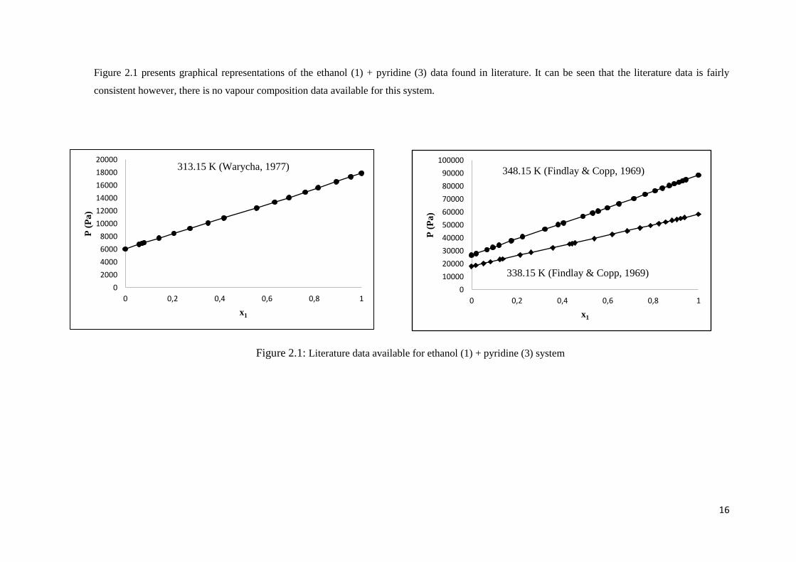
Figure 2.1 presents graphical representations of the ethanol (1) + pyridine (3) data found in literature. It can be seen that the literature data is fairly

consistent however, there is no vapour composition data available for this system.

0

10000

20000

30000

40000

50000

60000

70000

80000

90000

100000

0 0,2 0,4 0,6 0,8 1

P (

Pa

)

x1

0

2000

4000

6000

8000

10000

12000

14000

16000

18000

20000

0 0,2 0,4 0,6 0,8 1

P (

Pa

)

x1

313.15 K (Warycha, 1977) 348.15 K (Findlay & Copp, 1969)

338.15 K (Findlay & Copp, 1969)

Figure 2.1: Literature data available for ethanol (1) + pyridine (3) system

17

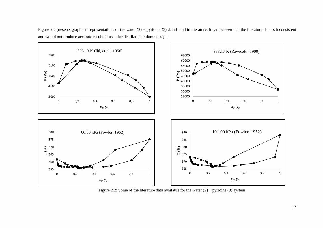
Figure 2.2 presents graphical representations of the water (2) + pyridine (3) data found in literature. It can be seen that the literature data is inconsistent

and would not produce accurate results if used for distillation column design.

Figure 2.2: Some of the literature data available for the water (2) + pyridine (3) system

25000

30000

35000

40000

45000

50000

55000

60000

65000

0 0,2 0,4 0,6 0,8 1

P (

Pa

)

x3, y3

353.17 K (Zawidzki, 1900)

365

370

375

380

385

390

0 0,2 0,4 0,6 0,8 1

T (

K)

x3, y3

101.00 kPa (Fowler, 1952)

355

360

365

370

375

380

0 0,2 0,4 0,6 0,8 1

T (

K)

x3, y3

66.60 kPa (Fowler, 1952)

3600

4100

4600

5100

5600

0 0,2 0,4 0,6 0,8 1

P (

Pa

)

x3, y3

303.13 K (Ibl, et al., 1956)

18

2.2 Residue Curve Map

A residue curve map (RCM) describes the equilibrium relationships for a ternary mixture. Each

curve represents the liquid residue composition with time obtained from a one stage batch

distillation. The process designed in this study is continuous (the RCM can also be used to

illustrate continuous distillation). Residue curves are used to test the feasibility of separation

schemes and therefore are a valuable tool in designing separation schemes for distillation

processes. These diagrams are commonly used for studying ternary mixtures which cannot be

easily separated by distillation due to azeotropic points.

An extensive literature review indicated that the Non-Random Two Liquid (NRTL) activity

coefficient model was the appropriate thermodynamic model for the binary/ternary combinations

studied. Hence, the RCM for the ethanol (1) + water (2) + pyridine (3) system was generated on

Aspen Plus® using the NRTL activity coefficient model and is displayed in Figure 2.3. This

Figure was generated at a series of pressures to study the phase behaviour at various conditions.

The RCM presented in Figure 2.3 is at a pressure of 80 kPa. The remaining diagrams display a

similar trend with slight differences in temperature and composition.

Table 2.1 presents the boiling points for the system ethanol (1) + water (2) + pyridine (3) with the

azeotropic compositions included. In the RCM, the unstable node is referred to the point where

all residue curves in a region originate and typically has the lowest boiling point; the stable node

refers to the point where all residue curves terminate and has the highest boiling point in the

region; lastly, the saddle is the point which residue curves move toward and then away from and

consists of intermediate boiling components in the region (Seader, et al., 2011).

Table 2.1: Boiling points and azeotropic compositions for the system ethanol (1) + water (2) +

pyridine (3) generated on Aspen Plus® at 80 kPa.

Mole Fraction

Temperature (K) Classification Ethanol Water Pyridine

345.58 Saddle 1 0 0

366.67 Stable Node 0 1 0

380.38 Stable Node 0 0 1

345.44 Unstable Node 0.9012 0.0988 0

360.57 Saddle 0 0.7443 0.2557

19


model with azeotropes (mole fractions) at 80 kPa, ( ) indicates azeotropic compositions.

Each apex in Figure 2.3 represents the pure chemical component, labelled with the pure

component boiling temperature at 80 kPa (ethanol: 345.58 K; water: 366.67 K; pyridine: 380.38

K). The RCM shows an arrow on each residue curve. The arrows point from a lower boiling point

to a higher boiling point. All residue curves originate from the ethanol/water azeotrope (lowest

boiling point, 345.44 K). One of the curves terminates at the other azeotrope (water/pyridine,

which has a higher boiling point, 360.57 K) and is a special residue curve, called a distillation

boundary (indicated by bold green line) because it divides the ternary diagram into two separate

regions. This boundary cannot be crossed or is extremely difficult to cross thus; restricting the

possible distillation products. All residue curves in region 1 terminate at the pyridine apex, which

has the highest boiling point (380.38 K) for that region. All residue curves in region 2 terminate

at the water apex, whose boiling point (366.67 K) is the highest for that region (Seader, et al.,

2011).

From the RCM, it can be seen that if a mixture composition point lies in region 1, pure pyridine

can be obtained by conventional distillation since the residue curves move toward and terminate

at the pyridine apex. The output from the top of the distillation column will result at/near the

ethanol/water azeotropic composition. Enhanced distillation processes are then required to the

break the ethanol/water azeotrope to separate these components.

Region 1

Region 2

20

If a mixture composition point lies in region 2, the process becomes more complex because the

pyridine and ethanol apex lie on the other side of the distillation boundary hence the stream cannot

be separated by conventional distillation into pure components. Instead the product streams will

consist of an ethanol/water mixture at the top of the column and a water/pyridine mixture at the

bottom of the column. Enhanced distillation processes will be required to break both azeotropes.

The RCM displayed in Figure 2.4 below includes the stream compositions of interest. Streams 5,

12, 27 and 29 are obtained from the process flow diagram developed by NECSA (Figure 1.2).

Stream 36 is the mixed stream (a combination of streams 5, 12, 27 and 29).


model with stream compositions and azeotropes (mole fractions) at 80 kPa, (O) indicates stream

compositions, ( ) indicates azeotropic compositions.

Stream 5

Ethanol : 0.0060 Water : 0.8271 Pyridine: 0.1669

Stream 12

Ethanol : 0.9142 Water : 0.0571 Pyridine : 0.0287

Stream 27


Nitrogen: 0.0035

Stream 29


Nitrogen : 0.0333

Stream 36 Ethanol : 0.8105 Water : 0.1450 Pyridine : 0.0445

Region 2

Tolerance Point


Region 1

D

B

21

Since the objective of this project is to separate the waste stream into pure components: pyridine,

ethanol and nitrogen, it is therefore necessary to ensure that the combined waste stream (streams

5, 12, 27 & 29 combined to stream 36) has a final composition which still lies in region 1 so that

the separation scheme developed will be less complex, costly and energy intensive as opposed to

the separation scheme required if the final composition lies in region 2. The tolerance point as

shown in Figure 2.4 indicates the composition with the maximum allowable water concentration

to remain in region 1 so as to obtain a high pyridine mole purity after distillation.

If more water is added to stream 36, its composition will be altered and its location on the diagram

will move. This new location is called the tolerance point. It was found that a mass addition of

540 kg/hr of water to stream 36 will still enable good separation to meet the objectives. However,

as the water content is increased above this composition, a high pyridine mole purity is still

possible but the recovery decreases resulting in a loss of pyridine. This is not acceptable since the

complexing agent is the most vital component in this study. If a larger amount of water is added

to stream 36 such that it is shifted into region 2, the separation of pyridine via conventional

methods is not possible due to the azeotrope it forms with water. Therefore, an enhanced

distillation process such as extractive distillation, azeotropic distillation, pervaporation, etc. is

required to obtain pure pyridine which would increase costs and complicate the design process.

From Figure 2.4, it can be seen that stream 36 does lie in region 1. Therefore, pure pyridine can

be obtained by conventional distillation since the residue curves move toward and terminate at

the pyridine apex (output from the bottom of the distillation column represented by point B). The

output from the top of the distillation column will result at/near the ethanol/water azeotropic

composition (point D). The ethanol/water mixture will then be separated using an enhanced

separation technique. Extractive distillation and pervaporation were selected for further

investigation since these are common and simple processes, less energy intensive than the

alternatives and can handle the feed capacity. These processes are discussed in the sections which

follow.

2.3 Extractive Distillation

Extractive distillation utilises a solvent with a high boiling point to alter the relative volatility of

the azeotropic mixture, thereby allowing the separation of components. A second column is

required to recover and recycle the solvent. It is essential that the most suitable solvent (one which

minimises the solvent to feed ratio and liquid load) is selected to economically design the

extractive distillation column. The four kinds of solvents used for distillation include solid salt,

liquid solvent, the combination of liquid and solid salt, ionic liquid (Lie, et al., 2003).

22

The advantages of using the solid salt includes good separation ability and low energy

consumption due to the lower solvent to feed ratio required (Gil, et al., 2008). However, problems

are encountered with the dissolution reuse and transport of salt when used in industrial operation

(Lie, et al., 2003). With ionic liquids, insufficient knowledge exists on the optimal properties and

their implementation in real process systems (Gutierrez H, 2013). The combination of a salt and

liquid solvent allows utilising the advantages of both components such as good separation ability

(solid salt) and easy solvent (liquid solvent). Furthermore, the combination produces a greater

effect on the relative volatility of the ethanol/water system and the quantity of the solvent to

recycle is reduced thereby lowering energy consumption (Gil, et al., 2008). However, solvent may

be entrained along with the product and many salts are corrosive to the equipment and tend to

decompose at high temperatures (Lie, et al., 2003). The liquid solvent is the most common

operation used with the most effective solvents being ethylene glycol and glycerol. Glycerol has

a higher selectivity, higher heat of vaporisation, and higher boiling point hence it is able to achieve

a high purity product more effectively than ethylene glycol under the same operating conditions,

but requires a higher energy consumption and produces higher temperatures at the reboiler which

may lead to thermal degradation of the mixture (Gil, et al., 2014). Ethylene glycol was selected

as the solvent for further investigation since it is a common and simple process, is less energy

intensive than its alternative liquid solvents and ionic liquids and contains no unwanted

entrainment (solid salt) into the product or equipment. For the column design and optimisation,

simulation results are presented in chapter 6.

2.4 Pervaporation

“Pervaporation involves the separation of liquid mixtures by partial vaporization through a dense

non-porous membrane” (Kujawski, 2000). Pervaporation operates independently from the vapour

liquid equilibrium, avoiding the issue of the ethanol/water azeotrope. Hence, the addition of a

third component is not required thereby reducing the energy consumption and operating costs

associated with solvent recovery (Kujawski, 2000). Figure 2.5 presents a schematic representation

of a pervaporation unit. A liquid mixture is fed into one side of the membrane. Transportation of

the mixture is driven by a pressure gradient across the membrane. The permeate undergoes a

phase change and is removed as a vapour while the retentate retains its liquid form. The pressure

gradient involves the difference in partial pressure between the liquid feed solution and the

permeate vapour (Xu, 2001). The feed mixture is usually at atmospheric pressure, therefore in

order to generate a good driving force, a vacuum is drawn on the permeate side and hence requires

condensing before recycling or reuse of components.

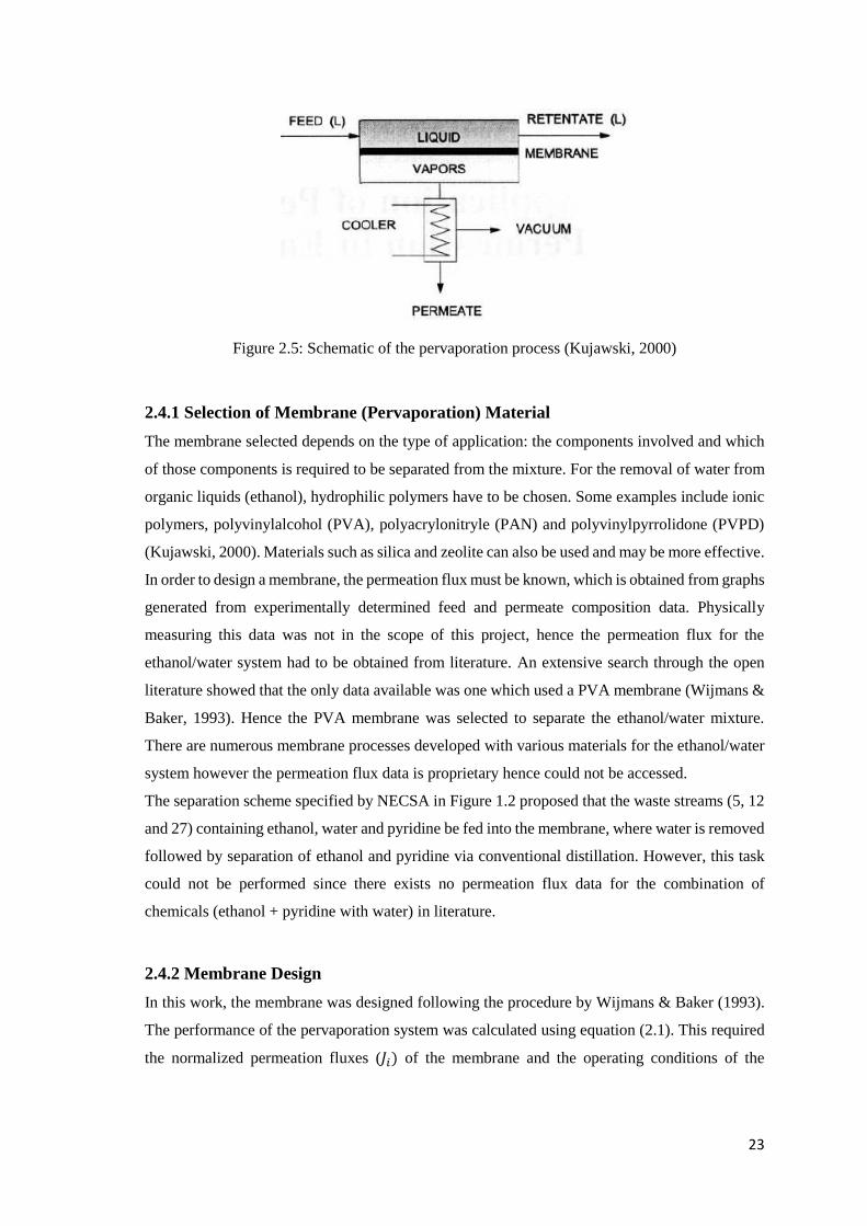
23

Figure 2.5: Schematic of the pervaporation process (Kujawski, 2000)

2.4.1 Selection of Membrane (Pervaporation) Material

The membrane selected depends on the type of application: the components involved and which

of those components is required to be separated from the mixture. For the removal of water from

organic liquids (ethanol), hydrophilic polymers have to be chosen. Some examples include ionic

polymers, polyvinylalcohol (PVA), polyacrylonitryle (PAN) and polyvinylpyrrolidone (PVPD)

(Kujawski, 2000). Materials such as silica and zeolite can also be used and may be more effective.

In order to design a membrane, the permeation flux must be known, which is obtained from graphs

generated from experimentally determined feed and permeate composition data. Physically

measuring this data was not in the scope of this project, hence the permeation flux for the

ethanol/water system had to be obtained from literature. An extensive search through the open

literature showed that the only data available was one which used a PVA membrane (Wijmans &

Baker, 1993). Hence the PVA membrane was selected to separate the ethanol/water mixture.

There are numerous membrane processes developed with various materials for the ethanol/water

system however the permeation flux data is proprietary hence could not be accessed.

The separation scheme specified by NECSA in Figure 1.2 proposed that the waste streams (5, 12

and 27) containing ethanol, water and pyridine be fed into the membrane, where water is removed

followed by separation of ethanol and pyridine via conventional distillation. However, this task

could not be performed since there exists no permeation flux data for the combination of

chemicals (ethanol + pyridine with water) in literature.

2.4.2 Membrane Design

In this work, the membrane was designed following the procedure by Wijmans & Baker (1993).

The performance of the pervaporation system was calculated using equation (2.1). This required

the normalized permeation fluxes (𝐽𝑖) of the membrane and the operating conditions of the

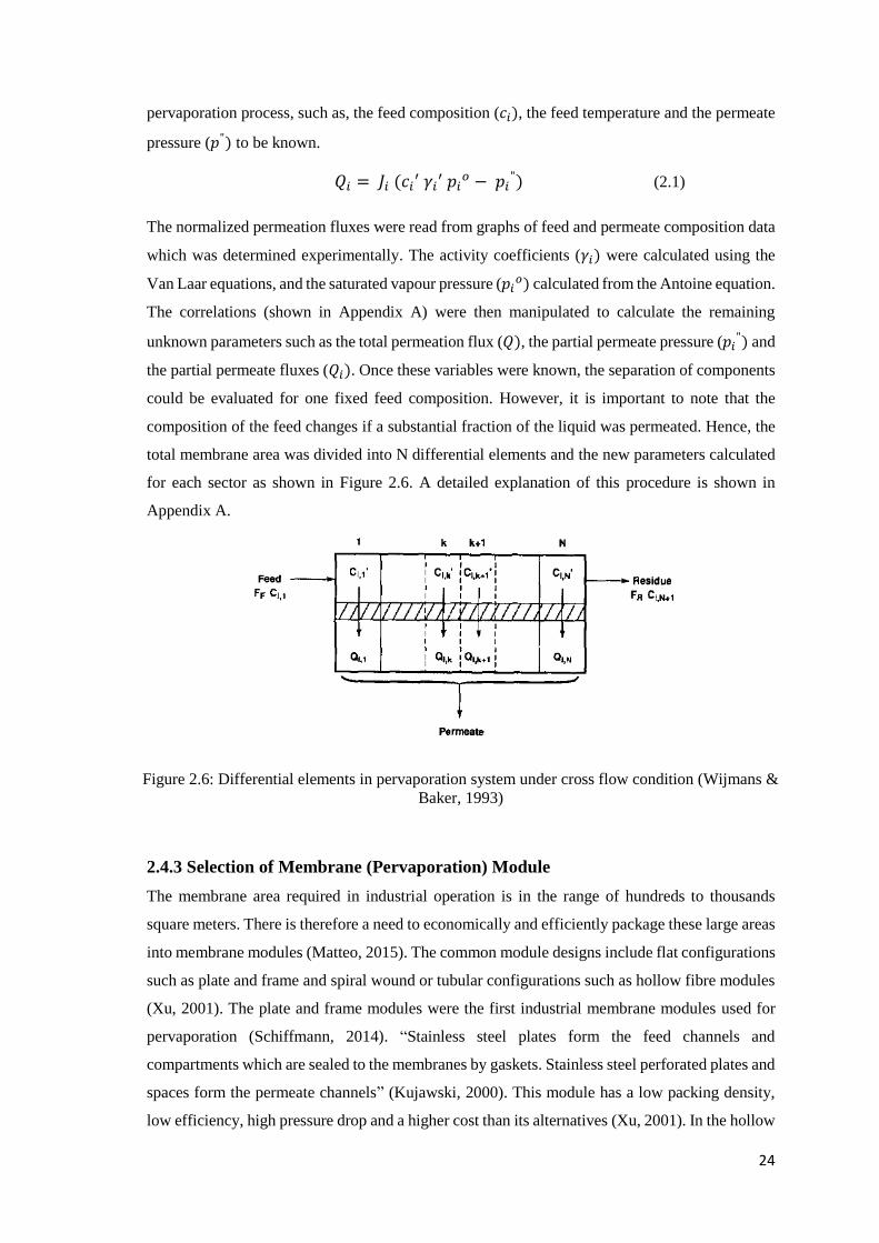
24

pervaporation process, such as, the feed composition (𝑐𝑖), the feed temperature and the permeate

pressure (𝑝") to be known.

The normalized permeation fluxes were read from graphs of feed and permeate composition data

which was determined experimentally. The activity coefficients (𝛾𝑖) were calculated using the

Van Laar equations, and the saturated vapour pressure (𝑝𝑖𝑜) calculated from the Antoine equation.

The correlations (shown in Appendix A) were then manipulated to calculate the remaining

unknown parameters such as the total permeation flux (𝑄), the partial permeate pressure (𝑝𝑖") and

the partial permeate fluxes (𝑄𝑖). Once these variables were known, the separation of components

could be evaluated for one fixed feed composition. However, it is important to note that the

composition of the feed changes if a substantial fraction of the liquid was permeated. Hence, the

total membrane area was divided into N differential elements and the new parameters calculated

for each sector as shown in Figure 2.6. A detailed explanation of this procedure is shown in

Appendix A.

2.4.3 Selection of Membrane (Pervaporation) Module

The membrane area required in industrial operation is in the range of hundreds to thousands

square meters. There is therefore a need to economically and efficiently package these large areas

into membrane modules (Matteo, 2015). The common module designs include flat configurations

such as plate and frame and spiral wound or tubular configurations such as hollow fibre modules

(Xu, 2001). The plate and frame modules were the first industrial membrane modules used for

pervaporation (Schiffmann, 2014). “Stainless steel plates form the feed channels and

compartments which are sealed to the membranes by gaskets. Stainless steel perforated plates and

spaces form the permeate channels” (Kujawski, 2000). This module has a low packing density,

low efficiency, high pressure drop and a higher cost than its alternatives (Xu, 2001). In the hollow

Figure 2.6: Differential elements in pervaporation system under cross flow condition (Wijmans &

Baker, 1993)

𝑄𝑖 = 𝐽𝑖 (𝑐𝑖′ 𝛾𝑖

′ 𝑝𝑖𝑜 − 𝑝𝑖

") (2.1)

25

fibre module, fibres are combined in bundles and sealed at the ends with impermeable material.

Feed flows through the fibres and the permeate is removed from the shell. This module has

irreversible fouling, easy breakage due to high flexibility of fibres, high temperature drop and

increased installation costs (Schiffmann, 2014). Figure 2.7 presents a schematic of the spiral

wound module. Membrane envelopes are wound around a perforated central collection tube

which is placed inside a tubular pressure vessel. This design is the simplest and most widely used,

as it allows for easy cleaning, has a high packing density and is inexpensive. The major problem

with this design is the high pressure drop (Xu, 2001). The spiral wound module was selected for

further investigation since it is simpler and less expensive than its alternatives.

Figure 2.7: Spiral wound module (Xu, 2001)

Figure 2.8 illustrates an example of the module configuration expected. The number of modules

in series and parallel depend on the capacity of the flow rate and the membrane and module

specifications selected. The total flow rate would be divided by the number of parallel modules

and fed in equal amounts to each parallel arrangement as shown in the Figure. The retentate

exiting each module becomes the feed to the next module, this is represented by the black lines

in the diagram. The permeate exits the bottom of each module and accumulates to a single stream,

this is represented by the red lines in the diagram.

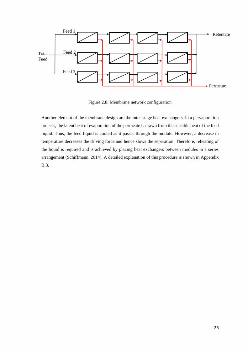
26

Another element of the membrane design are the inter-stage heat exchangers. In a pervaporation

process, the latent heat of evaporation of the permeate is drawn from the sensible heat of the feed

liquid. Thus, the feed liquid is cooled as it passes through the module. However, a decrease in

temperature decreases the driving force and hence slows the separation. Therefore, reheating of

the liquid is required and is achieved by placing heat exchangers between modules in a series

arrangement (Schiffmann, 2014). A detailed explanation of this procedure is shown in Appendix

B.3.

Figure 2.8: Membrane network configuration

Permeate

Retentate

Total

Feed

Feed 3

Feed 2

Feed 1

27

CHAPTER 3: THEORETICAL MODELLING

The aim of data modelling is to select a thermodynamic model that accurately represents the

measured VLE data and is able to extrapolate to conditions beyond the measurement conditions.

Such modelling is necessary for the process design and optimisation. This chapter presents a brief

review of the thermodynamic principles for low pressure VLE data correlation and analysis.

3.1 Analysis of VLE Data

Phase equilibria data can be described from the understanding of a basic principle which becomes

valid only when the phases are at equilibrium. This principle is represented by equation 3.1 for a

vapour–liquid system.

𝑓𝑖𝑙(T,P,𝑥𝑖) = 𝑓𝑖

𝑣 (T,P,𝑦𝑖) (3.1)

The symbols 𝑓𝑖𝑙and 𝑓𝑖

𝑣 represent the fugacities of the liquid and vapour phases, respectively. The

fugacities are related to temperature, pressure and composition via the use of the activity

coefficient (𝛾) and the fugacity coefficient (Φ). This resulted in the development of the following

analytical methods to describe the phase equilibria data: the combined method (𝛾− Φ), the direct

(Φ –Φ) method and the modern direct method.

The combined method uses both the activity coefficient and the fugacity coefficient to describe

the non-idealities of the liquid and vapour phases respectively according to the following

correlation:

𝑓𝑖𝑙= 𝑥𝑖𝛾𝑖𝑓𝑖

𝑜 = 𝑓𝑖𝑣 = 𝑦𝑖ф̂𝑖

𝑣P (3.2)

The symbol 𝑓𝑖𝑜 is the fugacity of pure component i at standard state and ф̂𝑖

𝑣 is the fugacity

coefficient of component i in the vapour phase. The fugacity coefficient is generated from an

equation of state while the activity coefficient is generated from the excess Gibbs energy model.

Although the (𝛾− ф) method allows for accurate analysis of non-ideal mixtures due to the ability

of the activity coefficient model to generate large excess Gibbs free energies of mixing (Orbey &

Sandler, 1998), this model has significant drawbacks. The details of these disadvantages can be

found in the following texts: Raal & Muhlbaüer (1998) and Orbey & Sandler (1998).

This resulted in the development of the (ф – ф) method. This method uses the fugacity coefficient

to describe the non-idealities in both the vapour and liquid phases as follows:

𝑓𝑖𝑙= 𝑥𝑖ф̂𝑖

𝑙 = 𝑓𝑖

𝑣 = 𝑦𝑖ф̂𝑖𝑣

(3.3)

28

This method had difficulties describing data for complex systems hence the modern direct method

was developed. This method uses equation of state (EoS) mixing rules to incorporate activity

coefficients (excess free energy models) into the fugacity coefficients of the liquid and vapour

phases. The relationship between the EoS and the activity coefficient described by Orbey and

Sandler (1998) is represented by equation 3.4:

𝛾𝑖= [ф̂𝑖(T,P, 𝑥𝑖)/ф𝑖(T,P)] (3.4)

The symbols ф̂𝑖(𝑇,P,𝑥𝑖) is the fugacity coefficient of species i in the mixture, and ф𝑖(𝑇,𝑃) is the

pure component fugacity coefficient. Equation 3.5 gives the correlation for the molar excess

Gibbs free energy. The combination of equations (3.4) and (3.5) results in the mixture EoS models

which are capable of describing high degrees of non-ideality.

𝐺𝐸

𝑅𝑇= ∑𝑥𝑖𝑙𝑛𝛾𝑖 (3.5)

In an ideal system, the vapour phase is represented by an ideal gas and the liquid phase by an

ideal solution. This is accomplished by setting Φ𝑖 and 𝛾𝑖 to a value of one.

An extensive search was conducted which showed that the popular models used in literature and

simulation packages to regress data for the systems studied are the following activity coefficient

models: NRTL, Wilson and UNIQUAC (Universal Quasi-Chemical) along with an ideal vapour

phase. However, in this study, an EoS needed to be incorporated due to the high pressure used for

one of the units in the separation scheme (flash vessel at 1930 kPa). Hence, both the combined

method and the modern direct method were used to regress the measured VLE data in this study.

For the derivation of all the equations above, and definitions of fugacity coefficient and activity

coefficient, the reader is referred to the following texts Raal and Mühlbauer (1998), Orbey and

Sandler (1998), Kontogeorgis & Folas (2009) and Seader, et al.(2011).

3.2 Thermodynamic Models used in this study

The thermodynamic models used in describing the liquid and vapour phases will be discussed in

this section. The modern direct method was used in conjunction with a configuration of models

which included an equation of state, a mixing rule, an alpha function and an activity coefficient

model. The direct method comprised of an ideal vapour phase and an activity coefficient model.

These models are common and widely used hence only a brief discussion is presented.

29

The development of the EoS models is described by Seader and Henley (2011) as follows: the

simplest EoS is the ideal gas law. This model does not take into account the volume occupied by

the molecules and the interaction forces. Hence, alternative EoS models developed attempt to

provide a correction for these two factors. The first successful EoS developed for a non-ideal gas

was the van der Waals equation. This model proposed that all species have equal reduced molar

volumes at the same reduced temperature and reduced pressure. This was used to develop the

compressibility factor which accounts for differences in molecular shape. The Redlich Kwong

(RK) equation was then developed as an improvement to the van der Waals equation. A

modification was made to this equation where a parameter was added (acentric factor, ) resulting

in the Soave-Redlich-Kwong (SRK) equation. This model is simple, accurate and provides a good

fit to vapour pressure data thereby improving the ability of the equation to predict liquid phase

properties. A modification was made to the RK and SRK models which resulted in the Peng-

Robinson (PR) EoS. This model displayed improvements in the critical region and accounted for

liquid molar volume. Hence the PR EoS was selected for data regression and is presented in the

sections to follow.

3.2.1 Peng-Robinson Cubic Equation of State

The popular EoS is reported as:

𝑃 = 𝑅𝑇

𝑉−𝑏−

𝑎𝑐 𝛼

𝑣(𝑣+𝑏)+𝑏(𝑣−𝑏) (3.6)

𝑎𝑐 = 0.45724 (𝑅2𝑇𝑐

2

𝑃𝑐) (3.7)

𝑏 = 0.07780 (𝑅𝑇𝑐

𝑃𝑐) (3.8)

The parameters a (temperature dependent) is related to the intermolecular attraction force of

molecules and b (temperature independent) accounts for the molecular size of the molecule. The

alpha function which was used in equation (3.6) is represented as follows:

𝛼 = [1 + (0.37464) + 1.54226𝜔 − 0.2699𝜔2 × (1 + 𝑇𝑟0.5]2 (3.9)

𝜔 is the acentric factor. The Peng-Robinson EoS is widely used in industry but it has some

limitations. Some of which include not accurately predicting data for long chain molecules and

predicting saturation pressure for vapour liquid equilibrium data. A detailed review of the

shortcomings can be found in the following text Abbott (1979). Due to these drawbacks, the

model has been modified to improve upon the predictive capabilities. This will be discussed in

the sections to follow.

30

3.2.2 Mathias Copeman Alpha Function

Alpha functions were developed to improve the ability of EoS models in representing the

thermodynamic properties of components at various conditions. The original alpha function

which was implemented into the Peng-Robinson EoS was developed by Soave (1972). This alpha

function however could not predict vapour pressures at low temperatures, including temperatures

above the critical point (Twu, et al., 2002). Thus, alternative alpha functions were developed

seeking to improve the vapour pressure prediction.

There are numerous correlations available hence in this study, various alpha functions were

incorporated into the Peng-Robinson EoS in order to investigate the performance of alpha

functions, with the aim of selecting the most suitable function. The Mathias-Copeman (MC) alpha

function was used as it produced the best improvement to the vapour pressure fit. The MC alpha

function is represented by the following correlation:

𝛼𝑖(𝑇) = [1 + 𝐶1,𝑖(1 − √𝑇𝑅,𝑖) + 𝐶2,𝑖(1 − √𝑇𝑅,𝑖)2+ 𝐶3,𝑖(1 − √𝑇𝑅,𝑖)

3]2

(3.10)

The function parameters are represented by 𝐶1,𝑖, 𝐶2,𝑖 and 𝐶3,𝑖, with 𝑇𝑅,𝑖signifying the reduced

temperature of species i. These parameters are generated through the regression of vapour

pressure data.

3.2.3 Mixing rules: Wong-Sandler

EoS models were initially developed for pure substances. In order to account for mixtures, these

correlations were extended through the use of the mixing and combining rules (Sadus, 2012).

Hence, these rules correlate the properties of the pure component to those of the mixture. The

standard was the Van der Waals one-fluid mixing rules represented by equations 3.11 and 3.12:

a= ∑∑𝑥𝑖𝑥𝑗𝑎𝑖𝑗 (3.11)

b= ∑∑𝑥𝑖𝑥𝑗𝑏𝑖𝑗 (3.12)

The symbols 𝑎𝑖𝑗 and 𝑏𝑖𝑗 are evaluated through the use of combining rules, which essentially

optimise the agreement between theory and experimental data. The combining rules are correlated

as follows:

𝑎𝑖𝑗=√𝑎𝑖𝑖𝑎𝑗𝑗 (1−𝑘𝑖𝑗) (3.13)

𝑏𝑖𝑗= 1

2(𝑏𝑖𝑖+𝑏𝑗𝑗)(1−𝑙𝑖𝑗)

(3.14)

The symbols 𝑘𝑖𝑗 and 𝑙𝑖𝑗 represent the binary interaction parameters. 𝑘𝑖𝑗 is calculated from fitting

EoS predictions to experimental VLE data. 𝑙𝑖𝑗 is usually set equal to zero (Seader, et al., 2011).

31

The 𝑘𝑖𝑗 parameter has the ability to determine the strength of the intermolecular forces in a

mixture as shown in Table 3.1. The closer 𝑘𝑖𝑗 is to zero, the better the agreement between

experimental and predicted data (Kontogeorgis & Folas, 2009). Non-ideal behaviour is

characterised by the azeotropes.

Table 3.1: Significance of 𝑘𝑖𝑗 binary interaction parameter

𝑘𝑗𝑖 = 0 System is ideal exhibiting Raoults law (forces between like and unlike

molecules are equal)

𝑘𝑗𝑖 > 0 System exhibits a positive deviation from Raoults law (forces between like

molecules are stronger)

𝑘𝑗𝑖 < 0 System exhibits a negative deviation from Raoults law (forces between

unlike molecules are stronger)

The original form of the Peng-Robinson EoS utilises the Van der Waal one fluid mixing rules.

This combination effectively describes phase equilibria data for mixtures of hydrocarbons and

hydrocarbons with inorganic gases (Sandler, 1994) but is only useful in mixtures with moderate

solution non-ideality. Most industrial chemical mixtures however have a relatively higher degree

of non-ideality. Thus, in order to account for this shortcoming, mixing rules that combine EoS

models with activity coefficient models were developed.

The first mixing rule (combining EoS models with activity coefficient models) was developed by

Huron and Vidal (1979). This was achieved through empirical means, by dictating that the EoS

of the mixture at the density of the liquid should behave in the same manner as an activity

coefficient model (Orbey & Sandler, 1998). The mixing rule combines the excess Gibbs energy

of mixing for an EoS and that of an activity coefficient model as follows:

𝐺𝑦𝐸(T,P= ∞,x)= 𝐺𝐸𝑜𝑆

𝐸 (T, P = ∞,x) (3.15)

The subscripts EoS and 𝛾 refer to an equation of state and activity coefficient model, respectively.

The superscript E represents the excess energy.

This mixing rule was partially successful but had significant flaws. It had difficulty describing

mixtures that the Van der Waal one fluid mixing rule could effectively describe. Furthermore, it

failed to satisfy the composition dependency, which is required for the second virial coefficient.

This led to the development of the modified Huron – Vidal second order model (Sandler, 1994).

However, this mixing rule also failed due to its inability to satisfy the composition dependency.

32

These flaws were overcome with the development of the mixing rules by Wong and Sandler

(1992) which succeeded where Huron and Vidal (1979) failed. This was achieved through the use

of the excess Helmholtz free –energy (𝐴𝐸) at an infinite pressure. The mixing rule parameters are

formulated based on the following condition:

𝐴𝐸𝑜𝑆𝐸 =𝐴𝑦

𝐸 (T,P= ∞,𝑥𝑖)= 𝐴𝑦𝐸 (T,low,P,𝑥𝑖)= 𝐺𝑦

𝐸 (T,low,P, 𝑥𝑖) (3.16)

The resulting mixing rules were then correlated as follows:

𝑎𝑚=RT(Z) 𝑊

(1−𝑊) (3.17)

𝑏𝑚= 𝑍

(1−𝑊) (3.18)

Z= ∑∑𝑥𝑖𝑥𝑗 (b – 𝑎

𝑅𝑇)𝑖𝑗 (3.19)

W= ∑𝑥𝑖 𝑎𝑖

𝑏𝑖 𝑅𝑇+

𝐺(𝐸)(𝑥𝑖)

𝜎 𝑅𝑇 (3.20)

The constant 𝜎 depends on the equation of state being used and for the Peng-Robinson EoS, this

constant is correlated as:

σ= −11

√2 ln(1+√2) (3.21)

The mixing rule uses the following combining rules as restrictions for the EoS parameters a and

b:

(𝑏𝑖𝑗 − 𝑎𝑖𝑗

𝑅𝑇) =

1

2 [(

𝑏𝑖𝑖− 𝑎𝑖𝑗

𝑅𝑇) + (𝑏𝑗𝑗 −

𝑎𝑗𝑗

𝑅𝑇)] (1 − 𝑘𝑖𝑗) (3.22)

3.2.4 Activity Coefficient Models

In order to effectively assess the properties of non-ideal liquid mixtures an activity coefficient

model is utilised, which relates the Gibbs excess function to the liquid composition. Presented is

a brief description of the activity coefficient models used in this study.

The Wilson Activity Coefficient Model

The Wilson activity coefficient model (Wilson, 1964) is based on the concept of local

composition, which occurs within a liquid solution. Local compositions are areas in the mixture

that differ from the overall mixture composition. It accounts for the non-random molecular

orientations in the solution which results from differences in molecular size and intermolecular

forces. The Wilson equation has two limitations: the inability to predict immiscibility and not

being able depict maximum or minimum activity coefficient - mole fraction relationships (Nelson,

2012).

33

The Non-Random Two Liquid (NRTL) Activity Coefficient Model

The NRTL equation (Renon & Prausnitz, 1968) was then developed as an improved local

composition model. This equation is capable of predicting both partially miscible and completely

miscible systems and is suitable for highly-non-ideal systems. The NRTL equation for the excess

Gibbs energy for a binary mixture is:

𝐺𝐸

𝑅𝑇 = 𝑥𝑖𝑥𝑗 (

𝜏𝑗𝑖𝐺𝑗𝑖

𝑥𝑖+ 𝑥𝑗𝐺𝑗𝑖+

𝜏𝑖𝑗𝐺𝑖𝑗

𝑥𝑗+ 𝑥𝑖𝐺𝑖𝑗) (3.23)

The parameters 𝜏𝑗𝑖 and 𝜏𝑖𝑗 are adjustable and (𝐺𝑖𝑗=(−𝜎𝜏𝑖𝑗)). The activity coefficient of the model is

represented by

𝑙𝑛𝛾𝑖 = 𝑥𝑗2[𝜏𝑗𝑖 (

𝐺𝑗𝑖

𝑥𝑖+ 𝑥𝑗𝐺𝑗𝑖) 2 +

𝜏𝑖𝑗𝐺𝑖𝑗

(𝑥𝑗+ 𝑥𝑖𝐺𝑖𝑗)2] (3.24)

While ln𝛾𝑗 is obtained through interchanging the subscripts in equation (3.24). In the software

package Aspen Plus® V 8.4, which was employed in the regression of all experimental data in

this work, the NRTL model is defined as follows:

𝜏𝑖𝑗 = 𝑎𝑖𝑗 + 𝑏𝑖𝑗

𝑇+ 𝑒𝑖𝑗 ln 𝑇 + 𝑓𝑖𝑗𝑇 (3.25)

The symbols τij is the interaction binary parameter and 𝑎𝑖𝑗, 𝑏𝑖𝑗, 𝑒𝑖𝑗, 𝑓𝑖𝑗 are obtained through the

regression of the experimental data. The parameters 𝑒𝑖𝑗, 𝑓𝑖𝑗 were not used in this work, and as

such were assigned a value of zero. The non-randomness parameter is correlated by the following

formulae:

𝛼𝑖𝑗 = 𝑐𝑖𝑗 + 𝑑𝑖𝑗(𝑇 − 273.15 𝐾) (3.26)

The symbol 𝑑𝑖𝑗 is set to zero, thus resulting in the reduction of the above correlation into an

identity of the form (𝛼𝑖𝑗= 𝑐𝑖𝑗). The parameter 𝑐𝑖𝑗 is selected based on the chemical characteristics

of the components which make up the mixture. Suitable guidelines for values of 𝛼𝑖𝑗 are shown in

Table 3.2. Model parameters obtained from literature and VLE applications using the Dortmund

Data Bank are stored in Aspen Plus® for over 1000 component pairs. The fixed parameter 𝑐𝑖𝑗

selected in this work was the literature value stored in Aspen Plus® for each binary system (0.3

for ethanol/pyridine and 0.69 for water/pyridine).

34

Table 3.2: Suitable guideline for 𝛼𝑖𝑗 parameter (Seader, et al., 2011)

𝛼𝑗𝑖 = 0.20 Hydrocarbons and polar, non-associated species

𝛼𝑗𝑖 = 0.30

Non-polar compounds, except fluorocarbons and paraffins; nonpolar and

polar, non-associated species; polar species that exhibit negative deviations

from Raoult’s law and moderate positive deviations; mixtures of water and

polar non-associated species.

𝛼𝑗𝑖 = 0.40 Saturated hydrocarbons and homolog perfluorocarbons.

𝛼𝑗𝑖 = 0.47 Alcohols or other strongly self-associated species with nonpolar species.

The Universal Quasi-Chemical (UNIQUAC) Equation

The UNIQUAC equation (Abrams & Prausnitz, 1975) comprises a combinatorial part and a

residual part. The combinational part accounts for the variances in sizes and shapes of the

molecules. The residual part accounts for the intermolecular forces between the molecules.

UNIQUAC utilises local area fraction as the prime concentration variable as opposed to local

volume fractions and local mole fractions used for Wilson and NRTL. The disadvantages of this

equation are its algebraic complexity and the requirement for pure component structural

parameters. These parameters however are available for the components of interest in this work.

Universal Functional Group Activity Coefficient Model (UNIFAC)

An estimation method was developed since liquid-phase activity coefficients are required for

design purposes even when experimental equilibria data are not available. This method is based

on functional groups instead of molecules. “For partial molar excess free energies and activity

coefficients, size parameters for each functional group and interaction parameters for each pair

are required. Size parameters can be calculated from theory. Interaction parameters are back-

calculated from existing phase-equilibria data and used with the size parameters to predict

properties of mixtures for which data are unavailable” (Seader, et al., 2011). Hence, the group

contribution methods rely on available data and functional groups to predict the data that is

unavailable. These are available for the systems in this study. Though, there are some

combinations for which this information is not available.

The UNIFAC (UNIQUAC Functional-group Activity Coefficients) group-contribution method

was first introduced by Fredenslund, Jones, and Prausnitz (1975) and developed further by

Fredenslund, Gmehling, and Rasmussen (1977), Gmehling, Rasmussen, and Fredenslund (1982),

35

and Larsen, Rasmussen, and Fredenslund (1987). The UNIFAC method is based on the

UNIQUAC equation, wherein the sum of the volume and area parameters of each functional group

in the molecule are used instead of the molecular volume and area parameters.

Gmehling et al. (1982) improved the group-contribution method by the introduction of a modified

UNIFAC method referred to as UNIFAC (Dortmund). The combinational part of the original

equation was modified due to mixtures having a range of molecular sizes and the temperature

dependence was replaced with a three-coefficient equation. Details of these modifications and

equations can be found in Seader, et al. (2011). These changes permit reliable predictions of

activity coefficients, azeotropic compositions and heats of mixing.

3.3 Vapour Liquid Equilibrium Prediction

The VLE data in this work is also compared to estimated data obtained from the Aspen Physical

Property System. Aspen Plus® stores physical property parameters for several components in

numerous databanks which are developed from the thermodynamic models inherent in the

package and data from the Dortmund Databank. These are the parameters retrieved to calculate

temperatures, pressures, mole compositions, etc. to generate the phase data required. The

predictive models used in this work are PSRK (Predictive Soave Redlich Kwong) and UNIFAC

(Universal Functional Group Activity Coefficient Model). Only a brief description is presented.

The list of equations and a more detailed explanation can be found in the following texts: Seader,

et al (2011) and AspenTech (2015).

3.3.1 Predictive Soave Redlich Kwong (PSRK)

For mixtures of nonpolar and slightly polar compounds, EoS models are useful. Gibbs free-energy

activity coefficient models are suitable for liquid subcritical nonpolar and polar compounds. For

mixtures that contain both polar compounds and supercritical gases, these methods are not

suitable. Hence, theoretically based mixing rules involving the SRK and PR EoS were developed

to describe vapour-liquid equilibria for such mixtures. Holderbaum and Gmehling (1991) further

developed these models for a range of applications by formulating a group-contribution equation

of state called the Predictive Soave Redlick Kwong (PSRK) model, which combines the SRK

equation of state with UNIFAC. The pure-component parameter a shown in equation 3.27

becomes temperature dependent in order to increase the ability of the SRK equation to predict

vapour pressure of polar compounds. A mixing rule that includes the UNIFAC model for non-

ideal effects was incorporated into the a parameter to account for mixtures of nonpolar, polar and

supercritical components.

𝑃 = 𝑅𝑇

𝑣−𝑏−

𝑎

𝑣2+𝑏𝑣 (3.27)

36

3.4 Data Regression

The proprietary software from Aspen Technology, Aspen Plus® V 8.4 was utilised for the

regression of experimental data and calculation of predicted data. An extensive literature review

showed that the popular models used in literature and simulation packages to regress data for the

systems studied are the following activity coefficient models: NRTL, Wilson and UNIQUAC

along with an ideal vapour phase. However, in this study, an EoS needed to be incorporated due

to the high pressure used for one of the units in the separation scheme (flash vessel at 1930 kPa).

Hence, the following configuration of models was used: Peng-Robinson EoS, with the

incorporation of the Mathias–Copeman alpha function, the Wong–Sandler mixing rules and an

activity coefficient model (Wilson, NRTL, UNIQUAC).

Furthermore, since the focus of this work was partly VLE measurement and design simulation

and costing; it was not the focus to provide too much time to data regression and modelling; the

popular and common models which proved adequate in correlating the data were used.

The objective function F is the sum of the squares of the errors between the calculated and

experimental values of one or more equilibrium-related properties. The optimal interaction

parameters in the chosen thermodynamic model are those that minimize the objective function.

In this study two different objective functions were used. For the ethanol + pyridine literature

data, the barker’s method shown in equation 3.28 was utilised since only the P-x data was

available.

𝜑 = ∑ (𝑃𝑗 − 𝑃𝑗𝑐𝑎𝑙𝑐)2𝑛𝑑𝑎𝑡𝑎

𝑗=1 (3.28)

𝑃𝑗 and 𝑃𝑗𝑐𝑎𝑙𝑐 represent the experimental and calculated values for the pressure respectively. The

ordinary least squares objective function was used for the water + pyridine literature data and in

the regression of all the measured VLE data. The objective function is calculated as follows:

𝐹 = 100

𝑁 [∑(𝑃𝑒𝑥𝑝− 𝑃𝑐𝑎𝑙

𝑃𝑒𝑥𝑝)2

+ ∑ (𝑦𝑒𝑥𝑝− 𝑦𝑐𝑎𝑙

𝑦𝑒𝑥𝑝)2

] (3.29)

𝑃𝑒𝑥𝑝,𝑦𝑒𝑥𝑝, 𝑃𝑐𝑎𝑙𝑐 and 𝑦𝑐𝑎𝑙𝑐 represent the experimental and calculated values for the pressure and

vapour compositions respectively.

37

CHAPTER 4: EXPERIMENTAL EQUIPMENT AND PROCEDURE

This chapter will focus on the description of the low-pressure vapour liquid equilibrium still and

the experimental procedure followed in this study. This includes calibrations, equilibrium cell

preparation, the measurement and control of temperature and pressure and analysis of the

equilibrium phases. For experimental VLE data that will be used in distillation design, any errors

in the measured data would not produce an accurate representation of the real system such as

predicting higher or lower product purities and energy demands. Therefore, the equipment used

should be correctly calibrated and operated; temperature, pressure and composition measurements

must be taken at the point where equilibrium actually occurs and the equilibrium should not be

disturbed whilst withdrawing the samples for analysis.

4.1 Low Pressure VLE Equipment

It is important to note that no single apparatus or single technique can measure VLE for all kinds

of systems, as the variation in temperatures, pressures and component characteristics (volatility,

corrosivity, thermal stability etc.) are too diverse. Thus, there exists a large array of experimental

techniques for VLE measurement. This section presents a brief description of the two methods

relevant in this study: static method and dynamic method. In the static method, the liquid mixture

is charged into the cell and agitated mechanically until equilibrium is reached with the vapour at

a fixed temperature. The static cells are usually immersed in a water bath at constant temperature

to produce isothermal data. For this method, complete degassing of the system is essential

(effective degassing can be very difficult and is the main source of error) since even minor

impurities could produce useless results (Bhownath, 2008). The dynamic method, also known as

the circulation method, involves the continuous separation of vapour phase from liquid phase

under steady state conditions and the recirculation of phases. The still can be operated under

isobaric or isothermal conditions. This method was employed to acquire the VLE data since it

allows measurements of high accuracy, it is simple, reliable and is typically used for low-pressure

VLE (Bhownath, 2008).

The VLE recirculating still of Raal and Mühlbauer (1998), which is based on the designs

of Heertjies (1960) and Yerazunis (1964), was used to acquire the binary VLE data. The

design of the still has not been changed drastically but some modifications have been

undertaken by Joseph, et al (2001), Ndlovu (2005) and Bhownath (2008) which will be

discussed in the sections to follow. Figure 4.1 presents a schematic representation of the

VLE recirculating still used in this study.

38

Figure 4.1: Schematic diagram of the VLE recirculating still (Bhownath, 2008)

A-temperature sensor, B-s/s wire mesh packing, C-equilibrium chamber, D-vacuum jacket, E-

magnetic stirrer, F- s/s spiral, G-Cottrell tube, H-vacuum jacket, I-glass tube, K-capillary, L-

reboiler, M-equilibrium chamber, N-inlet to condenser, O-drain valve, P-mixing tee, Q-glass

spiral, R-mixing chamber.

For the recirculating method, a binary liquid solution of 75 ml is initially charged into the boiling

chamber (L) and brought to boil via internal and external heaters. The internal heater consists of

a heating cartridge placed in the glass tube (I) which facilitates the boiling process. The external

heater contains nichrome wire that is wrapped around the boiling chamber and accounts for heat

39

losses to the environment. The boiling generates a vapour-liquid mixture that moves up through

the vacuum insulated Cottrell tube (G) and then downward through the vacuum jacketed

equilibrium chamber (M) where the phases disengage. The liquid phase channels down through

holes at the bottom of the equilibrium chamber to the liquid sampling point, while the vapour

flows upward around the equilibrium chamber and towards the condenser. The condensate is

collected in the vapour sampling point. Both phases recirculate via the reboiler. Equilibrium is

achieved when the plateau region (the region where the boiling temperature does not change for

a slight increase in the internal heater setting (Kneisl, et al., 1989)), is reached, there is a good

circulation rate in the still and a drop rate of approximately 60 drops per minute from the

condenser is observed. At this point, the contents in the still were left to circulate for a further 15

– 20 minutes to ensure equilibrium was actually achieved. There-after, the liquid and vapour

samples were withdrawn from the sampling points using a 1𝜇l gas tight GC syringe through a

chemically resistant spectrum. This ensured there was no effect on equilibrium temperature,

pressure and composition in the still during the withdrawal process. The samples were then

injected into a Shimadzu GC-2014 obtain the equilibrium composition measurements.

A Pt-100 temperature sensor (A), class B with an uncertainty of 0.1 K, housed in a glass tube (I)

shown in Figure 4.1 was used to measure the equilibrium temperature. The Pt-100 was connected

to a Hewlett-Packard (model 34401A) multi-meter that displayed resistance. For isothermal

measurements, temperature was maintained at fixed values by adjusting the pressure set point.

Decreasing the pressure reduced the temperature and increasing the pressure increased the

temperature. The pressure was controlled with a BUCHI model B-721 pressure controller that

used a two-way solenoid valve connected to a KNF vacuum pump and a vent to the atmosphere.

The vacuum pump was connected to a ballast tank to reduce pressure fluctuations. The allowable

operating pressure range in the still was 0 – 100 kPa. The pressure was measured using a WIKA

model P10 pressure transmitter with an uncertainty of 0.05 kPa.

The following modifications were made to the design of the VLE recirculating still of Raal and

Mühlbauer (1998):

Joseph et al. (2001) improved the isothermal operation of the still by implementing a

design based on pulse-width modulation of two solenoid valves with the aid of computer

control as opposed to manually changing the pressure controller setting to achieve the

desired temperature.

Ndlovu (2005) implemented an innovative design modification enabling the still to obtain

low pressure VLE data for partially miscible systems.

Bhownath (2008) combined the vapour condensate and liquid return lines into a tee

formation to increase the contact time and mixing time of the liquid mixture. A mixing

chamber was also added for further agitation of the liquid mixture. Resistance wire was

wrapped around the mixing tee and mixing chamber. These modifications allowed the

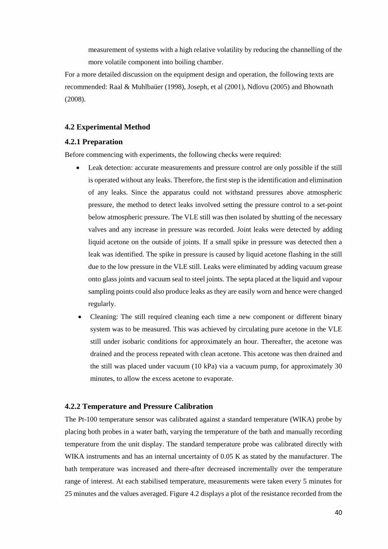
40

measurement of systems with a high relative volatility by reducing the channelling of the

more volatile component into boiling chamber.

For a more detailed discussion on the equipment design and operation, the following texts are

recommended: Raal & Muhlbaüer (1998), Joseph, et al (2001), Ndlovu (2005) and Bhownath

(2008).

4.2 Experimental Method

4.2.1 Preparation

Before commencing with experiments, the following checks were required:

Leak detection: accurate measurements and pressure control are only possible if the still

is operated without any leaks. Therefore, the first step is the identification and elimination

of any leaks. Since the apparatus could not withstand pressures above atmospheric

pressure, the method to detect leaks involved setting the pressure control to a set-point

below atmospheric pressure. The VLE still was then isolated by shutting of the necessary

valves and any increase in pressure was recorded. Joint leaks were detected by adding

liquid acetone on the outside of joints. If a small spike in pressure was detected then a

leak was identified. The spike in pressure is caused by liquid acetone flashing in the still

due to the low pressure in the VLE still. Leaks were eliminated by adding vacuum grease

onto glass joints and vacuum seal to steel joints. The septa placed at the liquid and vapour

sampling points could also produce leaks as they are easily worn and hence were changed

regularly.

Cleaning: The still required cleaning each time a new component or different binary

system was to be measured. This was achieved by circulating pure acetone in the VLE

still under isobaric conditions for approximately an hour. Thereafter, the acetone was

drained and the process repeated with clean acetone. This acetone was then drained and

the still was placed under vacuum (10 kPa) via a vacuum pump, for approximately 30

minutes, to allow the excess acetone to evaporate.

4.2.2 Temperature and Pressure Calibration

The Pt-100 temperature sensor was calibrated against a standard temperature (WIKA) probe by

placing both probes in a water bath, varying the temperature of the bath and manually recording

temperature from the unit display. The standard temperature probe was calibrated directly with

WIKA instruments and has an internal uncertainty of 0.05 K as stated by the manufacturer. The

bath temperature was increased and there-after decreased incrementally over the temperature

range of interest. At each stabilised temperature, measurements were taken every 5 minutes for

25 minutes and the values averaged. Figure 4.2 displays a plot of the resistance recorded from the

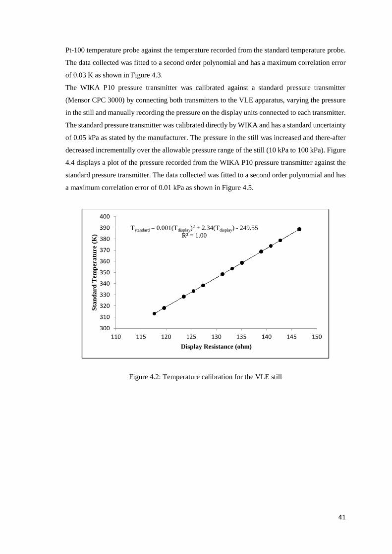
41

Pt-100 temperature probe against the temperature recorded from the standard temperature probe.

The data collected was fitted to a second order polynomial and has a maximum correlation error

of 0.03 K as shown in Figure 4.3.

The WIKA P10 pressure transmitter was calibrated against a standard pressure transmitter

(Mensor CPC 3000) by connecting both transmitters to the VLE apparatus, varying the pressure

in the still and manually recording the pressure on the display units connected to each transmitter.

The standard pressure transmitter was calibrated directly by WIKA and has a standard uncertainty

of 0.05 kPa as stated by the manufacturer. The pressure in the still was increased and there-after

decreased incrementally over the allowable pressure range of the still (10 kPa to 100 kPa). Figure

4.4 displays a plot of the pressure recorded from the WIKA P10 pressure transmitter against the

standard pressure transmitter. The data collected was fitted to a second order polynomial and has

a maximum correlation error of 0.01 kPa as shown in Figure 4.5.

Tstandard = 0.001(Tdisplay)2 + 2.34(Tdisplay) - 249.55

R² = 1.00

300

310

320

330

340

350

360

370

380

390

400

110 115 120 125 130 135 140 145 150

Sta

nd

ard

Tem

per

atu

re (

K)

Display Resistance (ohm)

Figure 4.2: Temperature calibration for the VLE still

42

Figure 4.3: Uncertainty in temperature calibration for the VLE still

Figure 4.4: Pressure calibration for the VLE still

-0,02

-0,01

-0,01

0,00

0,01

0,01

0,02

0,02

0,03

290 310 330 350 370 390 410

ΔT

(K

)

Standard Temperature (K)

Pstandard = 0.00003Pdisplay)2 + 0.99(Pdisplay) - 0.10

R² = 1.00

0

20

40

60

80

100

120

0 20 40 60 80 100 120

Sta

nd

ard

Pre

ssu

re (

kP

a)

Display Pressure (kPa)

43

Figure 4.5: Uncertainty in pressure calibration for the VLE still

4.2.3 Gas Chromatograph Thermal Conductivity Detector Calibration

A Shimadzu GC - 2014 with a thermal conductivity detector (TCD), which used helium as the

carrier gas was used to analyse compositions for the VLE systems studied in this project. A 2 m

× 2.2 mm Porapack Q column was utilised for component separation in the GC. The operating

conditions of the GC is presented in Table 4.1. The systems measured included: cyclohexane +

ethanol test system, ethanol + pyridine and water + pyridine. The purpose of measuring the test

system was to ensure the correct operation of the VLE apparatus and demonstrate the accuracy of

the experimental procedures.

Table 4.1: Operating conditions for the Shimadzu GC- 2014

System Cyclohexane + Ethanol

(Test System)

Ethanol + Pyridine Water + Pyridine

Gas flow rate (ml/min) 25 25 30

Oven Temperature (K) 453.15 483.15 493.15

Detector Temperature (K) 473.15 503.15 513.15

Injector Temperature (K) 473.15 503.15 513.15

The GC detector was calibrated following the method suggested by Raal & Muhlbaüer (1998)

which involved gravimetrically preparing binary liquid mixtures of known composition, injecting

the mixtures into the GC and plotting the ratio of the binary composition (x1/x2) against the ratio

of the peak area (A1/A2) generated after injection of sample into the GC. The samples were

prepared across the entire composition range in 4 ml vials. The volume of each sample injected

into the GC was 0.5 𝜇l. The response of the detector is defined by:

-0,012

-0,010

-0,008

-0,006

-0,004

-0,002

0,000

0,002

0,004

0,006

0,008

0 20 40 60 80 100 120Δ

P (

kP

a)

Standard Pressure (kPa)

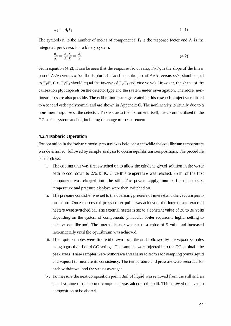
44

𝑛𝑖 = 𝐴𝑖𝐹𝑖 (4.1)

The symbols ni is the number of moles of component i, Fi is the response factor and Ai is the

integrated peak area. For a binary system:

𝑛1

𝑛2=

𝐴1

𝐴2

𝐹1

𝐹2=

𝑥1

𝑥2 (4.2)

From equation (4.2), it can be seen that the response factor ratio, F1/F2, is the slope of the linear

plot of A1/A2 versus x1/x2. If this plot is in fact linear, the plot of A2/A1 versus x2/x1 should equal

to F2/F1 (i.e. F1/F2 should equal the inverse of F2/F1 and vice versa). However, the shape of the

calibration plot depends on the detector type and the system under investigation. Therefore, non-

linear plots are also possible. The calibration charts generated in this research project were fitted

to a second order polynomial and are shown in Appendix C. The nonlinearity is usually due to a

non-linear response of the detector. This is due to the instrument itself, the column utilised in the

GC or the system studied, including the range of measurement.

4.2.4 Isobaric Operation

For operation in the isobaric mode, pressure was held constant while the equilibrium temperature

was determined, followed by sample analysis to obtain equilibrium compositions. The procedure

is as follows:

i. The cooling unit was first switched on to allow the ethylene glycol solution in the water

bath to cool down to 276.15 K. Once this temperature was reached, 75 ml of the first

component was charged into the still. The power supply, motors for the stirrers,

temperature and pressure displays were then switched on.

ii. The pressure controller was set to the operating pressure of interest and the vacuum pump

turned on. Once the desired pressure set point was achieved, the internal and external

heaters were switched on. The external heater is set to a constant value of 20 to 30 volts

depending on the system of components (a heavier boiler requires a higher setting to

achieve equilibrium). The internal heater was set to a value of 5 volts and increased

incrementally until the equilibrium was achieved.

iii. The liquid samples were first withdrawn from the still followed by the vapour samples

using a gas-tight liquid GC syringe. The samples were injected into the GC to obtain the

peak areas. Three samples were withdrawn and analysed from each sampling point (liquid

and vapour) to measure its consistency. The temperature and pressure were recorded for

each withdrawal and the values averaged.

iv. To measure the next composition point, 3ml of liquid was removed from the still and an

equal volume of the second component was added to the still. This allowed the system

composition to be altered.

45

v. Steps ii to iv were then repeated.

vi. The procedure was repeated until half of the phase diagram was complete. The still was

then cleaned with acetone and the procedure repeated starting with the second pure

component.

4.2.5 Isothermal Operation

To attain isothermal data, it is easier to operate the still in the isobaric mode so that the pressure

set point can be selected such that the equilibrium temperature is close to the desired operating

temperature (as opposed to a trial and error method). Once equilibrium was achieved as followed

by the steps in section 4.2.4, the isobaric operation was stopped and the temperature manually

adjusted to reach the temperature of interest by increasing or decreasing the pressure set point.

Once this temperature was reached and equilibrium was obtained, the liquid and vapour samples

were withdrawn then analysed and the procedure repeated in the same manner as the isobaric

operation.

46

CHAPTER 5: RESULTS AND DISCUSSION: EXPERIMENTAL

VLE DATA AND MODELLING

This chapter presents the results of the chemical characterisation of components, vapour pressure

and phase equilibrium data of the test system and the systems measured at new conditions. Also

included is a comparison of the measured data to literature data and modelled data obtained with

the use of suitable thermodynamic models.

The indicators used to judge the agreement between the experimental data and either referenced

or modelled data are the absolute average deviation (AAD) and absolute average relative

deviation (AARD) as represented by equations 5.1 and 5.2 respectively:

𝐴𝐴𝐷(�̅�) = 1

𝑁𝑝∑|�̅�𝑒𝑥𝑝 − �̅�𝑐𝑎𝑙𝑐| (5.1)

𝐴𝐴𝑅𝐷(�̅�) % = 1

𝑁𝑝∑|�̅�𝑒𝑥𝑝− �̅�𝑐𝑎𝑙𝑐|

�̅�𝑒𝑥𝑝 × 100 (5.2)

The symbols �̅�𝑒𝑥𝑝 and �̅�𝑐𝑎𝑙𝑐 are the experimental and calculated (or referenced) values of a

measured �̅� and Np is the total number of data points.

5.1 Chemical Characterisation

All the chemicals used in this work were analysed via the Shimadzu 2014 gas chromatograph, the

Atago Co Ltd., RX-7000∝ refractometer with a resolution of 0.0001 nD and the Anton Paar, DMA

5000 densitometer which has an accuracy to 0.0001 g/cm3. The experimental results and literature

values are shown in Table 5.1. All chemicals were used without further purification as no

significant impurities were observed.

Table 5.1: Chemical characterisation at 293.15 K

Refractive Index

(nD)

Density (g/cm3) GC (peak

area %)

Supplier and

specified purity

Component Exp Lit Exp Lit Exp Volume (%)

Cyclohexane 1.4263 1.4262e 0.7786 0.7785 f 99.94 Sigma Aldrich: 99.8

Ethanol 1.3613 1.3617c 0.7912 0.7910 g 99.91 ACS: 99.9

Pyridine 1.5102 1.5102h 0.9831 0.9832 d 99.94 Merck: 99.0

Water 1.333 1.333 a 0.9982 0.9982b 99.78 Distilled water

a (Harris, 2011) e (PubChem, 2015)

b (Allen, 2007) f (ChemicalBook, 2016) c (Haynes, 2011) g (Khattab, et al., 2012) d (PubChem, 2015) h (Kyte, et al., 1960)

47

5.2 Vapour Pressure Measurement

The combined expanded uncertainty for both temperature and pressure is calculated by the

method outlined by Taylor & Kuyatt (1994).

The combined standard uncertainty for temperature and pressure is calculated by:

𝑢𝐶 (𝑇) = ± √𝑢𝑐𝑎𝑙𝑖(𝜃)2 + 𝑢𝑟𝑒𝑝(𝜃)

2 + 𝑢𝑠𝑡𝑑(𝜃)2 + 𝑢𝑓𝑙𝑢𝑐𝑡(𝜃)

2 (5.3)

𝑢𝑐𝑎𝑙𝑖(𝜃) is the uncertainty induced by the calibration, 𝑢𝑟𝑒𝑝(𝜃) is the uncertainty due to

measurement repeatability, 𝑢𝑠𝑡𝑑(𝜃) is the standard uncertainty of the temperature or pressure

sensor as reported by the manufacturer and 𝑢𝑓𝑙𝑢𝑐𝑡(𝜃) is the fluctuation observed from the

temperature or pressure unit display. Refer to Table 5.7 for the numerical values of each term in

equation 5.3.

The combined expanded uncertainty is then calculated by multiplying the combined standard

uncertainty by a coverage factor of 2 and is displayed in Table 5.2. A more detailed description

of this method is presented in Appendix D.

Table 5.2: Combined expanded uncertainties for temperature and pressure

Uc (Temperature)a Uc (Pressure)a

0.3 K 0.10 kPa a Expanded uncertainties calculated using a coverage factor of k = 2

Figures 5.1 to 5.3 present the measured vapour pressure data for cyclohexane, ethanol and

pyridine respectively, all plotted against literature sources. These measurements were performed

to validate the calibrations for the temperature and pressure sensors. It can be seen that the vapour

pressure curves are linear indicating the stability of the components during the vapour pressure

measurements (no decomposition or polymerisation of the components were observed). Tables

5.3 to 5.5 contain the list of temperatures and pressures measured as well the deviation between

experimental data and literature. From the Tables, it can be seen that the percentage errors are

well below 1 % which indicates good agreement between the measured data and literature.

Regarding the difference in experimental temperature and literature temperature, some of the

values lie outside the calculated uncertainties. This is not unexpected since there is a deviation

between the literature sources as discussed below.

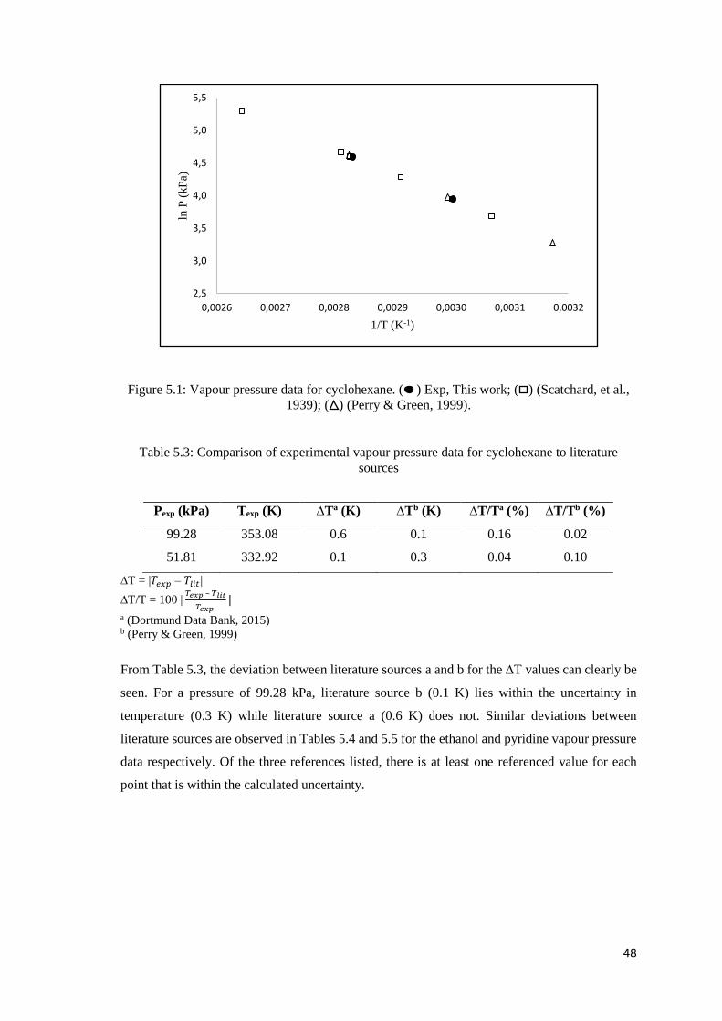
48

Figure 5.1: Vapour pressure data for cyclohexane. ( ) Exp, This work; ( ) (Scatchard, et al.,

1939); ( ) (Perry & Green, 1999).

Table 5.3: Comparison of experimental vapour pressure data for cyclohexane to literature

sources

∆T = |𝑇𝑒𝑥𝑝 – 𝑇𝑙𝑖𝑡 |

∆T/T = 100 | 𝑇𝑒𝑥𝑝 – 𝑇𝑙𝑖𝑡

𝑇𝑒𝑥𝑝 |

a (Dortmund Data Bank, 2015) b (Perry & Green, 1999)

From Table 5.3, the deviation between literature sources a and b for the ∆T values can clearly be

seen. For a pressure of 99.28 kPa, literature source b (0.1 K) lies within the uncertainty in

temperature (0.3 K) while literature source a (0.6 K) does not. Similar deviations between

literature sources are observed in Tables 5.4 and 5.5 for the ethanol and pyridine vapour pressure

data respectively. Of the three references listed, there is at least one referenced value for each

point that is within the calculated uncertainty.

2,5

3,0

3,5

4,0

4,5

5,0

5,5

0,0026 0,0027 0,0028 0,0029 0,0030 0,0031 0,0032

ln P

(kP

a)

1/T (K-1)

Pexp (kPa) Texp (K) ∆Ta (K) ∆Tb (K) ∆T/Ta (%) ∆T/Tb (%)

99.28 353.08 0.6 0.1 0.16 0.02

51.81 332.92 0.1 0.3 0.04 0.10

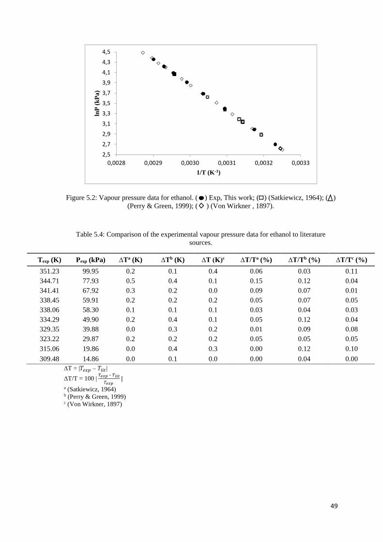
49

Figure 5.2: Vapour pressure data for ethanol. ( ) Exp, This work; ( ) (Satkiewicz, 1964); ( )

(Perry & Green, 1999); ( ) (Von Wirkner , 1897).

Table 5.4: Comparison of the experimental vapour pressure data for ethanol to literature

sources.

Texp (K) Pexp (kPa) ∆Ta (K) ∆Tb (K) ∆T (K)c ∆T/Ta (%) ∆T/Tb (%) ∆T/Tc (%)

351.23 99.95 0.2 0.1 0.4 0.06 0.03 0.11

344.71 77.93 0.5 0.4 0.1 0.15 0.12 0.04

341.41 67.92 0.3 0.2 0.0 0.09 0.07 0.01

338.45 59.91 0.2 0.2 0.2 0.05 0.07 0.05

338.06 58.30 0.1 0.1 0.1 0.03 0.04 0.03

334.29 49.90 0.2 0.4 0.1 0.05 0.12 0.04

329.35 39.88 0.0 0.3 0.2 0.01 0.09 0.08

323.22 29.87 0.2 0.2 0.2 0.05 0.05 0.05

315.06 19.86 0.0 0.4 0.3 0.00 0.12 0.10

309.48 14.86 0.0 0.1 0.0 0.00 0.04 0.00



𝑇𝑒𝑥𝑝 |

a (Satkiewicz, 1964) b (Perry & Green, 1999) c (Von Wirkner, 1897)

2,5

2,7

2,9

3,1

3,3

3,5

3,7

3,9

4,1

4,3

4,5

0,0028 0,0029 0,0030 0,0031 0,0032 0,0033

lnP

(k

Pa

)

1/T (K-1)

50

Figure 5.3: Vapour pressure data for pyridine. ( ) Exp, This work; ( ) (Chirico, et al., 1996);

( ) (Perry & Green, 1999); ( ) (McCullough, et al., 1957).

Table 5.5: Comparison of the experimental vapour pressure data for pyridine to literature

sources.

Texp (K) Pexp (kPa) ∆Ta (K) ∆Tb (K) ∆T (K)c ∆T/Ta (%) ∆T/Tb (%) ∆T/Tc (%)

383.76 89.94 0.4 0.1 0.5 0.12 0.03 0.12

379.86 79.93 0.4 0.1 0.5 0.11 0.04 0.12

375.62 69.92 0.4 0.0 0.4 0.11 0.01 0.11

370.83 59.91 0.3 0.6 0.3 0.08 0.17 0.09

365.36 49.90 0.2 0.7 0.2 0.05 0.20 0.06

358.79 39.88 0.2 0.4 0.2 0.06 0.12 0.07

350.91 29.87 0.0 0.3 0.1 0.01 0.08 0.02



𝑇𝑒𝑥𝑝 |

a (Chirico, et al., 1996) b (Perry & Green, 1999) c (McCullough, et al., 1957)

The AADs and AARDs for the experimental vapour pressure as well as the literature sources are

displayed in Table 5.6. The AARDs are well below 1 % and the AADs are below the experimental

uncertainties for the temperature measurement thereby indicating a good agreement between the

experimental and reference data.

2,8

3,0

3,2

3,4

3,6

3,8

4,0

4,2

4,4

4,6

4,8

0,0025 0,0026 0,0027 0,0028 0,0029 0,0030

lnP

(k

Pa

)

1/T (K-1)

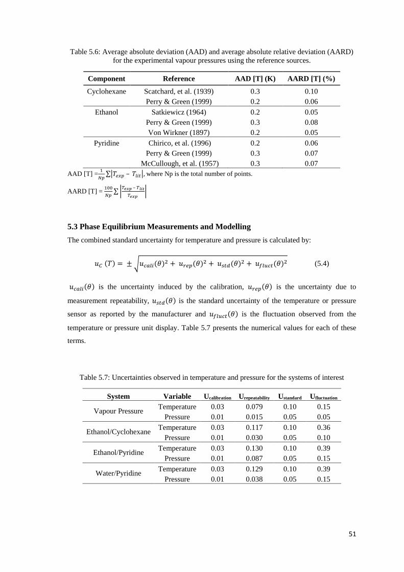
51

Table 5.6: Average absolute deviation (AAD) and average absolute relative deviation (AARD)

for the experimental vapour pressures using the reference sources.

Component Reference AAD [T] (K) AARD [T] (%)

Cyclohexane Scatchard, et al. (1939) 0.3 0.10

Perry & Green (1999) 0.2 0.06

Ethanol Satkiewicz (1964) 0.2 0.05

Perry & Green (1999) 0.3 0.08

Von Wirkner (1897) 0.2 0.05

Pyridine Chirico, et al. (1996) 0.2 0.06

Perry & Green (1999) 0.3 0.07

McCullough, et al. (1957) 0.3 0.07

AAD [T] =1

𝑁𝑝∑|𝑇𝑒𝑥𝑝 – 𝑇𝑙𝑖𝑡|, where Np is the total number of points.

AARD [T] = 100

𝑁𝑝∑ |

𝑇𝑒𝑥𝑝 – 𝑇𝑙𝑖𝑡

𝑇𝑒𝑥𝑝 |

5.3 Phase Equilibrium Measurements and Modelling

The combined standard uncertainty for temperature and pressure is calculated by:

𝑢𝐶 (𝑇) = ± √𝑢𝑐𝑎𝑙𝑖(𝜃)2 + 𝑢𝑟𝑒𝑝(𝜃)

2 + 𝑢𝑠𝑡𝑑(𝜃)2 + 𝑢𝑓𝑙𝑢𝑐𝑡(𝜃)

2 (5.4)

𝑢𝑐𝑎𝑙𝑖(𝜃) is the uncertainty induced by the calibration, 𝑢𝑟𝑒𝑝(𝜃) is the uncertainty due to

measurement repeatability, 𝑢𝑠𝑡𝑑(𝜃) is the standard uncertainty of the temperature or pressure

sensor as reported by the manufacturer and 𝑢𝑓𝑙𝑢𝑐𝑡(𝜃) is the fluctuation observed from the

temperature or pressure unit display. Table 5.7 presents the numerical values for each of these

terms.

Table 5.7: Uncertainties observed in temperature and pressure for the systems of interest

System Variable Ucalibration Urepeatability Ustandard Ufluctuation

Vapour Pressure Temperature 0.03 0.079 0.10 0.15

Pressure 0.01 0.015 0.05 0.05

Ethanol/Cyclohexane Temperature 0.03 0.117 0.10 0.36

Pressure 0.01 0.030 0.05 0.10

Ethanol/Pyridine Temperature 0.03 0.130 0.10 0.39

Pressure 0.01 0.087 0.05 0.15

Water/Pyridine Temperature 0.03 0.129 0.10 0.39

Pressure 0.01 0.038 0.05 0.15

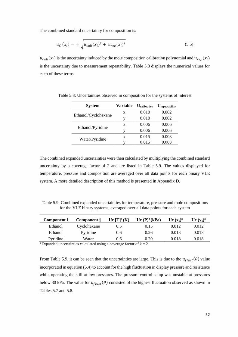
52

The combined standard uncertainty for composition is:

𝑢𝐶 (𝑥𝑖) = ± √𝑢𝑐𝑎𝑙𝑖(𝑥𝑖)2 + 𝑢𝑟𝑒𝑝(𝑥𝑖)

2 (5.5)

𝑢𝑐𝑎𝑙𝑖(𝑥𝑖) is the uncertainty induced by the mole composition calibration polynomial and 𝑢𝑟𝑒𝑝(𝑥𝑖)

is the uncertainty due to measurement repeatability. Table 5.8 displays the numerical values for

each of these terms.

Table 5.8: Uncertainties observed in composition for the systems of interest

System Variable Ucalibration Urepeatability

Ethanol/Cyclohexane x 0.010 0.002

y 0.010 0.002

Ethanol/Pyridine x 0.006 0.006

y 0.006 0.006

Water/Pyridine x 0.015 0.003

y 0.015 0.003

The combined expanded uncertainties were then calculated by multiplying the combined standard

uncertainty by a coverage factor of 2 and are listed in Table 5.9. The values displayed for

temperature, pressure and composition are averaged over all data points for each binary VLE

system. A more detailed description of this method is presented in Appendix D.

Table 5.9: Combined expanded uncertainties for temperature, pressure and mole compositions

for the VLE binary systems, averaged over all data points for each system

Component i Component j Uc [T]a (K) Uc (P)a (kPa) Uc (x1)a Uc (y1)a

Ethanol Cyclohexane 0.5 0.15 0.012 0.012

Ethanol Pyridine 0.6 0.26 0.013 0.013

Pyridine Water 0.6 0.20 0.018 0.018 a Expanded uncertainties calculated using a coverage factor of k = 2

From Table 5.9, it can be seen that the uncertainties are large. This is due to the 𝑢𝑓𝑙𝑢𝑐𝑡(𝜃) value

incorporated in equation (5.4) to account for the high fluctuation in display pressure and resistance

while operating the still at low pressures. The pressure control setup was unstable at pressures

below 30 kPa. The value for 𝑢𝑓𝑙𝑢𝑐𝑡(𝜃) consisted of the highest fluctuation observed as shown in

Tables 5.7 and 5.8.

53

5.3.1 Test System: Ethanol (1) + Cyclohexane (4)

Figures 5.4 to 5.7 present the isobaric and isothermal VLE data for the ethanol (1) + cyclohexane

(4) test system at 40 kPa and 313.15 K respectively. The purpose of measuring a test system is to

validate the accuracy of the experimental procedure by comparing the measured experimental

data to literature data.

Figure 5.4: Isobaric VLE data for the ethanol (1) + cyclohexane (4) system at 40 kPa. ( ) Exp,

This work; ( ) (Narasigadu, 2006); ( ) (Bhownath, 2008).

Figure 5.5: Isobaric x-y data for the ethanol (1) + cyclohexane (4) system at 40 kPa. ( )

Exp, This work; ( ) (Narasigadu, 2006); ( ) (Bhownath, 2008).

312

314

316

318

320

322

324

326

328

330

332

0 0,1 0,2 0,3 0,4 0,5 0,6 0,7 0,8 0,9 1

Tem

per

atu

re (

K)

x1, y1

0

0,1

0,2

0,3

0,4

0,5

0,6

0,7

0,8

0,9

1

0 0,1 0,2 0,3 0,4 0,5 0,6 0,7 0,8 0,9 1

y1

x1

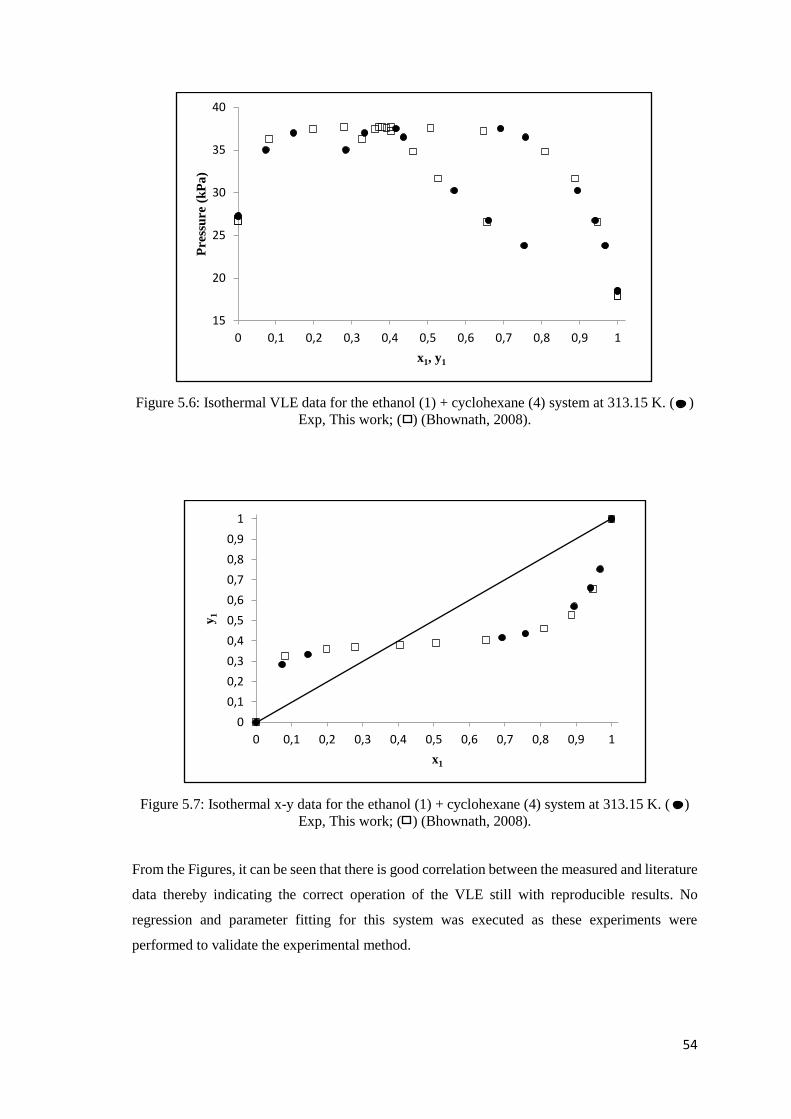
54

Figure 5.6: Isothermal VLE data for the ethanol (1) + cyclohexane (4) system at 313.15 K. ( )

Exp, This work; ( ) (Bhownath, 2008).

Figure 5.7: Isothermal x-y data for the ethanol (1) + cyclohexane (4) system at 313.15 K. ( )

Exp, This work; ( ) (Bhownath, 2008).

From the Figures, it can be seen that there is good correlation between the measured and literature

data thereby indicating the correct operation of the VLE still with reproducible results. No

regression and parameter fitting for this system was executed as these experiments were

performed to validate the experimental method.

15

20

25

30

35

40

0 0,1 0,2 0,3 0,4 0,5 0,6 0,7 0,8 0,9 1

Pre

ssu

re (

kP

a)

x1, y1

0

0,1

0,2

0,3

0,4

0,5

0,6

0,7

0,8

0,9

1

0 0,1 0,2 0,3 0,4 0,5 0,6 0,7 0,8 0,9 1

y1

x1

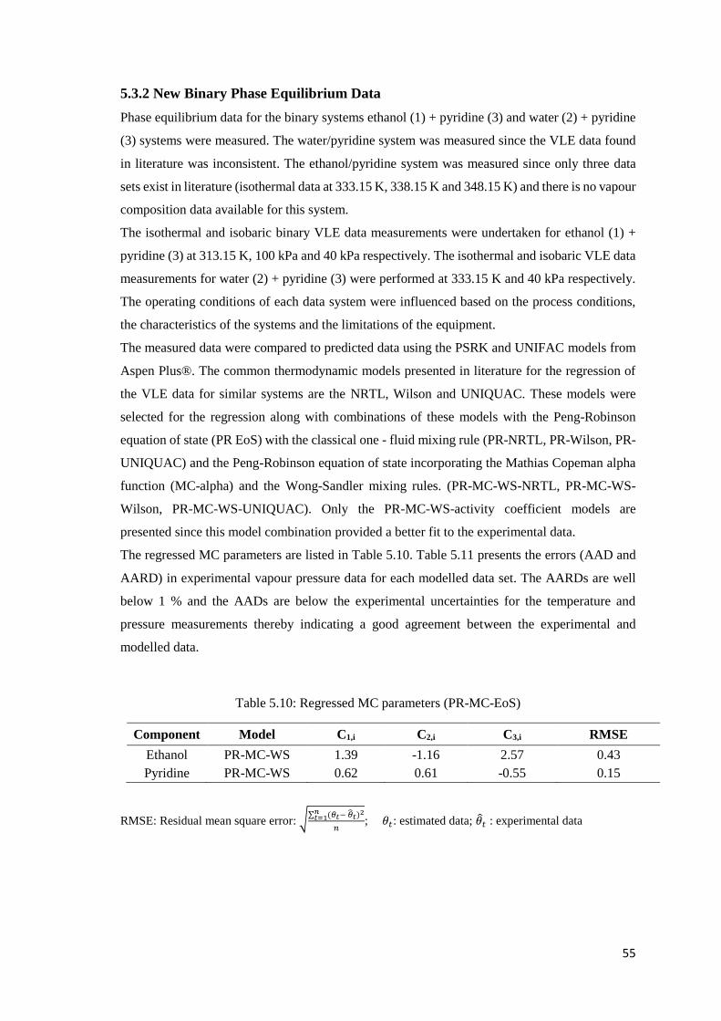
55

5.3.2 New Binary Phase Equilibrium Data

Phase equilibrium data for the binary systems ethanol (1) + pyridine (3) and water (2) + pyridine

(3) systems were measured. The water/pyridine system was measured since the VLE data found

in literature was inconsistent. The ethanol/pyridine system was measured since only three data

sets exist in literature (isothermal data at 333.15 K, 338.15 K and 348.15 K) and there is no vapour

composition data available for this system.

The isothermal and isobaric binary VLE data measurements were undertaken for ethanol (1) +

pyridine (3) at 313.15 K, 100 kPa and 40 kPa respectively. The isothermal and isobaric VLE data

measurements for water (2) + pyridine (3) were performed at 333.15 K and 40 kPa respectively.

The operating conditions of each data system were influenced based on the process conditions,

the characteristics of the systems and the limitations of the equipment.

The measured data were compared to predicted data using the PSRK and UNIFAC models from

Aspen Plus®. The common thermodynamic models presented in literature for the regression of

the VLE data for similar systems are the NRTL, Wilson and UNIQUAC. These models were

selected for the regression along with combinations of these models with the Peng-Robinson

equation of state (PR EoS) with the classical one - fluid mixing rule (PR-NRTL, PR-Wilson, PR-

UNIQUAC) and the Peng-Robinson equation of state incorporating the Mathias Copeman alpha

function (MC-alpha) and the Wong-Sandler mixing rules. (PR-MC-WS-NRTL, PR-MC-WS-

Wilson, PR-MC-WS-UNIQUAC). Only the PR-MC-WS-activity coefficient models are

presented since this model combination provided a better fit to the experimental data.

The regressed MC parameters are listed in Table 5.10. Table 5.11 presents the errors (AAD and

AARD) in experimental vapour pressure data for each modelled data set. The AARDs are well

below 1 % and the AADs are below the experimental uncertainties for the temperature and

pressure measurements thereby indicating a good agreement between the experimental and

modelled data.

Table 5.10: Regressed MC parameters (PR-MC-EoS)

Component Model C1,i C2,i C3,i RMSE

Ethanol PR-MC-WS 1.39 -1.16 2.57 0.43

Pyridine PR-MC-WS 0.62 0.61 -0.55 0.15

RMSE: Residual mean square error: √∑ (𝜃𝑡− �̂�𝑡)

2𝑛𝑡=1

𝑛; 𝜃𝑡: estimated data; �̂�𝑡 : experimental data

56

Table 5.11: Deviations in the experimental vapour pressure data from modelled data using the

PR EoS with the MC alpha function

Component Model AAD [P] (kPa) AARD [P] (%)

Ethanol PR-MC-WS 0.18 0.27

Pyridine PR-MC-WS 0.06 0.09

AAD [P] =1

𝑁𝑝∑|𝑃𝑒𝑥𝑝 – 𝑃𝑙𝑖𝑡|, Np is the total number of points.

AARD [P] = 100

𝑁𝑝∑ |

𝑃𝑒𝑥𝑝 – 𝑃𝑙𝑖𝑡

𝑃𝑒𝑥𝑝 |

In the sections to follow, the phase behaviour (P-x-y/T-x-y and x-y) for each binary system is

presented comprising the comparison of the experimental, literature and predicted data as well as

the comparison of the experimental and modelled data followed by the regressed model

parameters for each data set, the AADs and AARDs of each data point and the total AAD and

AARD for each system averaged over all data points.

Ethanol (1) + Pyridine (3) System: Comparison of Experimental Data to Predicted Data

and Literature Data

Figures 5.8 to 5.11 displays the experimental isobaric VLE data for the binary system of ethanol

(1) + pyridine (3) measured at 40 kPa and 100 kPa respectively while Figures 5.12 and 5.13

display the experimental isothermal VLE data measured at 313.15 K. The experimental

measurements are compared to literature data where they are available and the predictive models

from Aspen Plus®: PSRK and UNIFAC.

Figure 5.8: Isobaric VLE data for the ethanol (1) + pyridine (3) system at 40 kPa. ( ) Exp, This

work; ( ) PSRK model; (----) UNIFAC model.

325

330

335

340

345

350

355

360

365

0 0,1 0,2 0,3 0,4 0,5 0,6 0,7 0,8 0,9 1

Tem

per

ature

(K

)

x1, y1

57

Figure 5.9: Isobaric x-y data for the ethanol (1) + pyridine (3) system at 40 kPa. ( ) Exp, This

work; ( ) PSRK model; (----) UNIFAC model.

From Figures 5.8 and 5.9, it can be seen that the measured data correlate well with the predicted

data from Aspen Plus® for the isobaric system at 40 kPa.

Figure 5.10: Isobaric VLE data for the ethanol (1) + pyridine (3) system at 100 kPa. ( ) Exp,

This work; ( ) Exp, This work, Re-measured points; ( ) PSRK model; (----) UNIFAC model.

0

0,1

0,2

0,3

0,4

0,5

0,6

0,7

0,8

0,9

1

0 0,1 0,2 0,3 0,4 0,5 0,6 0,7 0,8 0,9 1

y1

x1

350

355

360

365

370

375

380

385

390

0 0,1 0,2 0,3 0,4 0,5 0,6 0,7 0,8 0,9 1

Tem

per

atu

re (

K)

x1, y1

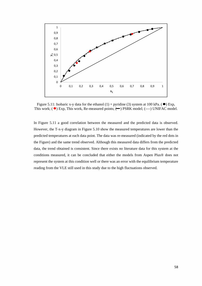
58

Figure 5.11: Isobaric x-y data for the ethanol (1) + pyridine (3) system at 100 kPa. ( ) Exp,

This work; ( ) Exp, This work, Re-measured points; ( ) PSRK model; (----) UNIFAC model.

In Figure 5.11 a good correlation between the measured and the predicted data is observed.

However, the T-x-y diagram in Figure 5.10 show the measured temperatures are lower than the

predicted temperatures at each data point. The data was re-measured (indicated by the red dots in

the Figure) and the same trend observed. Although this measured data differs from the predicted

data, the trend obtained is consistent. Since there exists no literature data for this system at the

conditions measured, it can be concluded that either the models from Aspen Plus® does not

represent the system at this condition well or there was an error with the equilibrium temperature

reading from the VLE still used in this study due to the high fluctuations observed.

0

0,1

0,2

0,3

0,4

0,5

0,6

0,7

0,8

0,9

1

0 0,1 0,2 0,3 0,4 0,5 0,6 0,7 0,8 0,9 1

y1

x1

59

Figure 5.12: Isothermal VLE data for the ethanol (1) + pyridine (3) system at 313.15 K. ( )

Exp, This work; ( ) PSRK model; (----) UNIFAC model; ( ) P-x data (Warycha, 1977).

Figure 5.13: Isothermal x-y data for the ethanol (1) + pyridine (3) system at 313.15 K. ( ) Exp,

This work; ( ) PSRK model; (----) UNIFAC model.

Figure 5.13 demonstrates a good correlation between the measured and the predicted data. The

P-x-y diagram in Figure 5.12 shows the measured pressures for the liquid compositions are higher

than the predicted pressures at each data point. However, the literature data measured by Warycha

(1977) follows the same trend as the data measured in this study. Warycha (1977) used the static

apparatus described by Janaszewsi, et al (1982) for the determination of the P-x data for the

ethanol/pyridine system. The data is measured by the following method: “A small amount of gas

5

7

9

11

13

15

17

19

0 0,1 0,2 0,3 0,4 0,5 0,6 0,7 0,8 0,9 1

Pre

ssu

re (

kP

a)

x1, y1

0

0,1

0,2

0,3

0,4

0,5

0,6

0,7

0,8

0,9

1

0 0,1 0,2 0,3 0,4 0,5 0,6 0,7 0,8 0,9 1

y1

x1

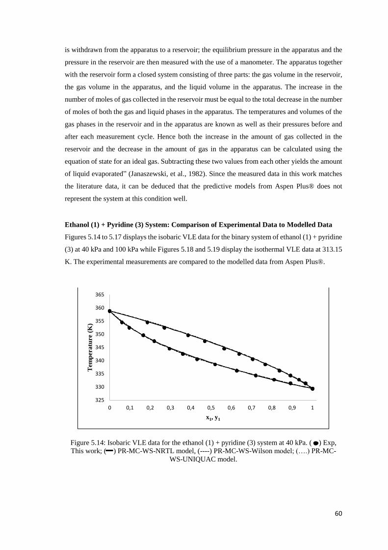
60

is withdrawn from the apparatus to a reservoir; the equilibrium pressure in the apparatus and the

pressure in the reservoir are then measured with the use of a manometer. The apparatus together

with the reservoir form a closed system consisting of three parts: the gas volume in the reservoir,

the gas volume in the apparatus, and the liquid volume in the apparatus. The increase in the

number of moles of gas collected in the reservoir must be equal to the total decrease in the number

of moles of both the gas and liquid phases in the apparatus. The temperatures and volumes of the

gas phases in the reservoir and in the apparatus are known as well as their pressures before and

after each measurement cycle. Hence both the increase in the amount of gas collected in the

reservoir and the decrease in the amount of gas in the apparatus can be calculated using the

equation of state for an ideal gas. Subtracting these two values from each other yields the amount

of liquid evaporated” (Janaszewski, et al., 1982). Since the measured data in this work matches

the literature data, it can be deduced that the predictive models from Aspen Plus® does not

represent the system at this condition well.

Ethanol (1) + Pyridine (3) System: Comparison of Experimental Data to Modelled Data

Figures 5.14 to 5.17 displays the isobaric VLE data for the binary system of ethanol (1) + pyridine

(3) at 40 kPa and 100 kPa while Figures 5.18 and 5.19 display the isothermal VLE data at 313.15

K. The experimental measurements are compared to the modelled data from Aspen Plus®.


This work; ( ) PR-MC-WS-NRTL model, (----) PR-MC-WS-Wilson model; (….) PR-MC-

WS-UNIQUAC model.

325

330

335

340

345

350

355

360

365

0 0,1 0,2 0,3 0,4 0,5 0,6 0,7 0,8 0,9 1

Tem

per

atu

re (

K)

x1, y1

61

Figure 5.15: Isobaric x-y data for the ethanol (1) + pyridine (3) system at 40 kPa. ( ) Exp, This

work; ( ) PR-MC-WS-NRTL model, (----) PR-MC-WS-Wilson model; (….) PR-MC-WS-

UNIQUAC model.

From Figures 5.14 and 5.15, it can be seen that the measured data correlate well with the

regressed data from Aspen Plus® for the 40 kPa isobaric system.



WS-UNIQUAC model.

0

0,1

0,2

0,3

0,4

0,5

0,6

0,7

0,8

0,9

1

0 0,1 0,2 0,3 0,4 0,5 0,6 0,7 0,8 0,9 1

y1

x1

345

350

355

360

365

370

375

380

385

390

0 0,1 0,2 0,3 0,4 0,5 0,6 0,7 0,8 0,9 1

Tem

per

atu

re (

K)

x1, y1

62

Figure 5.17: Isobaric x-y data for the ethanol (1) + pyridine (3) system at 100 kPa. ( ) Exp,


WS-UNIQUAC model.

In Figures 5.16 and 5.17, a fairly good correlation between the measured and the regressed data

is observed with slight discrepancies. Figure 5.16 show the measured temperatures are lower than

the regressed temperatures at each data point in the middle region while Figure 5.17 show the

measured vapour compositions are lower than the regressed data in the ethanol rich region.

However, as stated previously, the data was re-measured and the same trend observed.

Furthermore, although this measured data differs from the regressed data, the trend obtained is

consistent. Hence, it can be concluded that either the models from Aspen Plus® does not represent

the system at this condition well or there was an error with the equilibrium temperature reading

from the VLE still used in this study due to the high fluctuation observed.

0

0,1

0,2

0,3

0,4

0,5

0,6

0,7

0,8

0,9

1

0 0,1 0,2 0,3 0,4 0,5 0,6 0,7 0,8 0,9 1

y1

x1

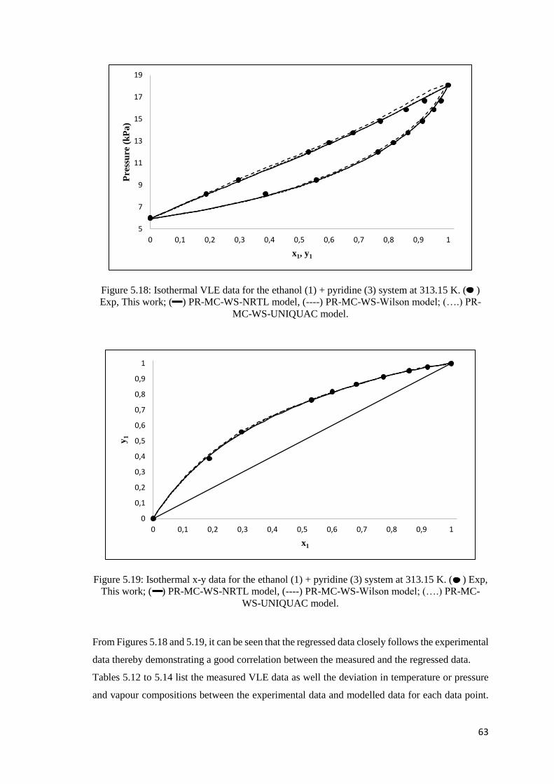
63

Figure 5.18: Isothermal VLE data for the ethanol (1) + pyridine (3) system at 313.15 K. ( )

Exp, This work; ( ) PR-MC-WS-NRTL model, (----) PR-MC-WS-Wilson model; (….) PR-

MC-WS-UNIQUAC model.

Figure 5.19: Isothermal x-y data for the ethanol (1) + pyridine (3) system at 313.15 K. ( ) Exp,


WS-UNIQUAC model.

From Figures 5.18 and 5.19, it can be seen that the regressed data closely follows the experimental

data thereby demonstrating a good correlation between the measured and the regressed data.

Tables 5.12 to 5.14 list the measured VLE data as well the deviation in temperature or pressure

and vapour compositions between the experimental data and modelled data for each data point.

5

7

9

11

13

15

17

19

0 0,1 0,2 0,3 0,4 0,5 0,6 0,7 0,8 0,9 1

Pre

ssu

re (

kP

a)

x1, y1

0

0,1

0,2

0,3

0,4

0,5

0,6

0,7

0,8

0,9

1

0 0,1 0,2 0,3 0,4 0,5 0,6 0,7 0,8 0,9 1

y1

x1

64

Tables 5.15 and 5.16 list the AADs and AARDs for each system averaged over all data points.

The total AARD in each Table represents the combined AARDs for temperature or pressure and

vapour compositions. Table 5.17 presents the regressed model parameters for each system.

65

Table 5.12: Comparison of the experimental VLE data to modelled data for the isobaric ethanol (1) + pyridine (3) system at 40 kPa

T (K) x1 y1 ∆Ta (K) ∆T/Ta (%) ∆y1a ∆y1/y1

a (%) ∆Tb (K) ∆T/Tb (%) ∆y1

b ∆y1/y1b

(%) ∆Tc (K) ∆T/Tc (%) ∆y1c ∆y1/y1

c (%)

354.52 0.060 0.186 0.1 0.03 0.003 1.83 0.3 0.09 0.001 0.42 0.4 011 0.003 1.52

352.48 0.096 0.270 0.2 0.05 0.003 1.01 0.3 0.09 0.002 0.65 0.4 0.11 0.000 0.03

349.60 0.166 0.387 0.1 0.04 0.013 3.45 0.2 0.04 0.020 5.12 0.1 0.03 0.020 5.05

347.40 0.220 0.469 0.0 0.00 0.009 1.99 0.2 0.04 0.020 4.23 0.2 0.04 0.020 4.35

344.50 0.295 0.565 0.4 0.11 0.004 0.74 0.1 0.04 0.017 2.96 0.1 0.03 0.018 3.12

342.51 0.361 0.639 0.4 0.11 0.002 0.27 0.1 0.04 0.010 1.56 0.1 0.02 0.011 1.64

340.57 0.431 0.705 0.4 0.11 0.005 0.73 0.2 0.05 0.004 0.55 0.1 0.04 0.004 0.53

338.56 0.520 0.767 0.2 0.04 0.002 0.24 0.1 0.02 0.007 0.88 0.1 0.01 0.006 0.73

336.18 0.627 0.837 0.1 0.02 0.001 0.18 0.2 0.05 0.003 0.31 0.2 0.05 0.001 0.12

334.37 0.721 0.892 0.1 0.03 0.002 0.20 0.1 0.03 0.002 0.20 0.1 0.03 0.003 0.31

332.77 0.811 0.933 0.2 0.07 0.001 0.13 0.0 0.00 0.000 0.04 0.1 0.02 0.001 0.05

331.41 0.892 0.966 0.3 0.10 0.002 0.19 0.2 0.05 0.000 0.00 0.2 0.07 0.000 0.01

∆T = |𝑇𝑒𝑥𝑝 – 𝑇𝑐𝑎𝑙𝑐 |

∆𝑦1 = |𝑦1𝑒𝑥𝑝 – 𝑦1𝑐𝑎𝑙𝑐 |

∆T/T = 100 | 𝑇𝑒𝑥𝑝 – 𝑇𝑐𝑎𝑙𝑐

𝑇𝑒𝑥𝑝 |

∆𝑦1/𝑦1 = 100 | 𝑦1𝑒𝑥𝑝 – 𝑦1𝑐𝑎𝑙𝑐

𝑦1𝑒𝑥𝑝 |

a PR-MC-WS-NRTL model b PR-MC-WS-Wilson model c PR-MC-WS-UNIQUAC model

From Table 5.12, the deviations are below the experimental uncertainties except for three points with slight deviations in vapour composition for the PR-

MC-WS-Wilson and PR-MC-WS-UNIQUAC models (∆𝑦 = 0.017 – 0.020 as opposed to the vapour composition uncertainty of 0.013).

66

Table 5.13: Comparison of the experimental VLE data to modelled data for the ethanol (1) + pyridine (3) system at 100 kPa

T (K) x1 y1 ∆Ta (K) ∆T/Ta (%) ∆y1a ∆y1/y1

a (%) ∆Tb (K) ∆T/Tb (%) ∆y1

b ∆y1/y1b

(%) ∆Tc (K) ∆T/Tc (%) ∆y1c ∆y1/y1

c (%)

383.89 0.031 0.116 0.3 0.07 0.006 5.18 0.5 0.13 0.013 10.92 0.4 0.11 0.010 8.52

380.09 0.085 0.209 0.1 0.03 0.046 21.86 0.4 0.10 0.042 19.98 0.2 0.06 0.045 21.69

377.16 0.134 0.304 0.0 0.00 0.051 16.94 0.1 0.03 0.054 17.84 0.0 0.00 0.057 18.70

374.39 0.182 0.384 0.2 0.05 0.051 13.36 0.1 0.03 0.060 15.55 0.0 0.01 0.061 15.93

371.64 0.233 0.479 0.5 0.14 0.029 6.09 0.2 0.06 0.041 8.62 0.2 0.06 0.042 8.73

368.68 0.292 0.572 0.9 0.25 0.007 1.28 0.5 0.14 0.020 3.58 0.6 0.16 0.021 3.60

366.06 0.355 0.635 0.9 0.28 0.010 1.52 0.6 0.16 0.021 3.30 0.7 0.19 0.021 3.35

363.97 0.432 0.705 0.6 0.18 0.008 1.08 0.3 0.07 0.014 2.04 0.4 0.10 0.016 2.24

361.67 0.509 0.760 0.6 0.16 0.010 1.37 0.3 0.09 0.012 1.61 0.4 0.12 0.015 1.95

358.97 0.614 0.832 0.4 0.11 0.005 0.61 0.3 0.10 0.003 0.32 0.4 0.12 0.006 0.78

357.22 0.688 0.872 0.3 0.08 0.004 0.51 0.3 0.09 0.002 0.23 0.4 0.11 0.006 0.66

355.52 0.771 0.918 0.1 0.03 0.003 0.35 0.1 0.01 0.003 0.33 0.2 0.04 0.001 0.06

353.92 0.853 0.951 0.0 0.00 0.002 0.21 0.3 0.08 0.001 0.14 0.1 0.03 0.002 0.17

352.90 0.899 0.971 0.1 0.02 0.005 0.55 0.3 0.09 0.002 0.17 0.0 0.01 0.002 0.24

∆T = |𝑇𝑒𝑥𝑝 – 𝑇𝑐𝑎𝑙𝑐 |


∆T/T = 100 | 𝑇𝑒𝑥𝑝 – 𝑇𝑐𝑎𝑙𝑐

𝑇𝑒𝑥𝑝 |

∆𝑦1/𝑦1 = 100 | 𝑦1𝑒𝑥𝑝 – 𝑦1𝑐𝑎𝑙𝑐

𝑦1𝑒𝑥𝑝 |


From table 5.13, the deviations are below the experimental uncertainties for the temperature measurement (∆𝑇 [𝐾] = 0.6) except for two points (∆𝑇 [𝐾]

= 0.9) for the PR-MC-WS-NRTL model and one point (∆𝑇 [𝐾] = 0.7) for the PR-MC-WS-UNIQUAC model. There is a greater discrepancy in the vapour

composition with an error in the range of ∆𝑦 = 0.014 – 0.061. However, as stated previously, the data was re-measured and the same consistent trend

67

observed. Therefore, it can be concluded that either the models from Aspen Plus® does not represent the system at this condition well or there was an

error with the equilibrium temperature reading from the VLE still used in this study due to the high fluctuation observed.

Table 5.14: Comparison of the experimental VLE data to modelled data for the ethanol (1) + pyridine (3) system at 313.15 K.

T (K) x1 y1 ∆Pa (K) ∆P/Pa (%) ∆y1a ∆y1/y1

a (%) ∆Pb (K) ∆P/Pb (%) ∆y1

b ∆y1/y1b

(%) ∆Pc (K) ∆P/Pc (%) ∆y1c ∆y1/y1

c (%)

8.20 0.188 0.387 0.01 0.08 0.018 4.63 0.00 0.04 0.027 7.04 0.01 0.09 0.019 4.98

9.45 0.296 0.558 0.01 0.08 0.011 1.93 0.00 0.00 0.001 0.21 0.01 0.06 0.005 0.87

12.00 0.532 0.764 0.01 0.07 0.001 0.17 0.00 0.00 0.001 0.16 0.01 0.05 0.001 0.19

12.85 0.601 0.817 0.01 0.08 0.005 0.59 0.00 0.02 0.005 0.60 0.01 0.07 0.004 0.48

13.76 0.681 0.865 0.00 0.00 0.003 0.33 0.01 0.05 0.004 0.46 0.00 0.00 0.003 0.38

14.81 0.773 0.914 0.01 0.03 0.001 0.11 0.01 0.08 0.001 0.08 0.00 0.03 0.002 0.17

15.86 0.859 0.952 0.01 0.05 0.000 0.02 0.02 0.12 0.002 0.25 0.01 0.05 0.000 0.04

16.66 0.920 0.977 0.01 0.04 0.001 0.06 0.02 0.12 0.001 0.10 0.01 0.04 0.000 0.03 ∆P = |𝑃𝑒𝑥𝑝 – 𝑃𝑐𝑎𝑙𝑐 |


∆P/P = 100 | 𝑃𝑒𝑥𝑝 – 𝑃𝑐𝑎𝑙𝑐

𝑃𝑒𝑥𝑝 |

∆𝑦1/𝑦1 = 100 | 𝑦1𝑒𝑥𝑝 – 𝑦1𝑐𝑎𝑙𝑐

𝑦1𝑒𝑥𝑝 |


From Table 5.14, the deviations are well below the experimental uncertainty for the pressure measurement. Regarding the deviations observed in vapour

composition, there is only one point for each model that lies outside the experimental uncertainty.

68

Table 5.15: Data regression deviations for the isobaric ethanol (1) + pyridine (3) binary system.

System Model AAD [T] (K) AARD [T] (%) AAD y1 AARD [y1] (%) AAD y2 AARD [y2] (%) Total AARD (%)

40 kPa PR-MC-WS-NRTL 0.2 0.05 0.004 0.90 0.003 1.44 2.39

PR-MC-WS-Wilson 0.1 0.04 0.007 1.42 0.006 1.70 3.16

PR-MC-WS-UNIQUAC 0.2 0.04 0.007 1.47 0.006 1.69 3.20

100 kPa PR-MC-WS-NRTL 0.3 0.09 0.017 5.05 0.015 4.75 9.90

PR-MC-WS-Wilson 0.3 0.08 0.020 6.03 0.018 4.37 10.47

PR-MC-WS-UNIQUAC 0.3 0.07 0.022 6.17 0.019 4.88 11.12

AAD [T] =1

𝑁𝑝∑|𝑇𝑒𝑥𝑝 – 𝑇𝑐𝑎𝑙𝑐|, Np is the total number of data points

AAD [𝑦𝑖] =1

𝑁𝑝∑ |𝑦1𝑒𝑥𝑝 – 𝑦1𝑐𝑎𝑙𝑐|,

AARD [T] = 100

𝑁𝑝∑ |

𝑇𝑒𝑥𝑝 – 𝑇𝑐𝑎𝑙𝑐

𝑇𝑒𝑥𝑝 |

AARD [𝑦𝑖] = 100

𝑁𝑝∑ |

𝑦1𝑒𝑥𝑝 – 𝑦1𝑐𝑎𝑙𝑐

𝑦1𝑒𝑥𝑝 |

In Tables 5.15 and 5.16, it can be seen that the thermodynamic model with the lowest deviation is the PR-MC-WS–NRTL for the 40 kPa system (AARD

= 2.39 %), hence the model parameters calculated with the use of this combination (displayed in Table 5.17) were selected for the ethanol (1) + pyridine

(3) system.

69

Table 5.16: Data regression deviations for the isothermal ethanol (1) + pyridine (3) binary system.

System Model AAD [P] (kPa) AARD [P] (%) AAD y1 AARD [y1] (%) AAD y2 AARD [y2] (%) Total AARD (%)

313.15 K PR-MC-WS-NRTL 0.01 0.04 0.005 1.00 0.004 1.97 3.01

PR-MC-WS-Wilson 0.01 0.05 0.005 1.13 0.004 2.27 3.45

PR-MC-WS-UNIQUAC 0.00 0.04 0.005 0.92 0.004 1.83 2.80

AAD [P] =1

𝑁𝑝∑|𝑃𝑒𝑥𝑝 – 𝑃𝑐𝑎𝑙𝑐|, Np is the total number of data points

AAD [𝑦1] =1

𝑁𝑝∑ |𝑦1𝑒𝑥𝑝 – 𝑦1𝑐𝑎𝑙𝑐|

AARD [P] = 100

𝑁𝑝∑ |

𝑃𝑒𝑥𝑝 – 𝑃𝑐𝑎𝑙𝑐

𝑃𝑒𝑥𝑝 |

AARD [𝑦1] = 100

𝑁𝑝∑ |


𝑦1𝑒𝑥𝑝 |

Table 5.17: Model parameters regressed for the ethanol (1) + pyridine (3) binary system

System Model kija aij

b ajib bij

b bjib αij

b RMSEc

40 kPa PR-MC-WS-NRTL 0.04 -383.65 607.83 0.3 3.43 PR-MC-WS-Wilson 0.21 -0.69 -2.26 562.68 460.71 3.59 PR-MC-WS-UNIQUAC 0.30 -518.79 357.35 3.41

100 kPa PR-MC-WS-NRTL 0.11 -456.65 684.21 0.3 11.25 PR-MC-WS-Wilson 0.36 1.52 -24.83 43.14 -4146.41 11.32 PR-MC-WS-UNIQUAC 0 -714.05 415.79 10.82

313.15 K PR-MC-WS-NRTL -0.30 64.34 165.97 0.3 4.14 PR-MC-WS-Wilson 0.35 2.91 -24.83 -388.22 -4146.41 11.32 PR-MC-WS-UNIQUAC 0.31 -474.50 338.36 4.01

a WS mixing rule parameter incorporated into the PR EoS b NRTL/Wilson/UNIQUAC model parameters c RMSE: Residual mean square error

70

Water (2) + Pyridine (3) System: Comparison of Experimental Data to Predicted

Data and Literature Data

Figures 5.20 to 5.23 displays the isobaric and isothermal VLE data for the binary system of water

(2) + pyridine (3) at 40 kPa and 333.15 K respectively. The experimental measurements are

compared to literature data where they are available and the predictive models from Aspen Plus®:

PSRK and UNIFAC.

Figure 5.20: Isobaric VLE data for the water (2) + pyridine (3) system at 40 kPa. ( ) Exp, This

work; ( ) Exp, This work, Re-measured points; ( ) Exp, This work, Re-measured points; ( )

PSRK model; (----) UNIFAC model; ( ) (Fowler, 1952).

Figure 5.21: Isobaric x-y data for the water (2) + pyridine (3) system at 40 kPa. ( ) Exp, This

work; ( ) Exp, This work, Re-measured points; ( ) Exp, This work, Re-measured points; ( )

PSRK model; (----) UNIFAC model; ( ) (Fowler, 1952).

342

344

346

348

350

352

354

356

358

360

362

0 0,1 0,2 0,3 0,4 0,5 0,6 0,7 0,8 0,9 1

Tem

per

atu

re (

K)

x3, y3

0

0,1

0,2

0,3

0,4

0,5

0,6

0,7

0,8

0,9

1

0 0,1 0,2 0,3 0,4 0,5 0,6 0,7 0,8 0,9 1

y3

x3

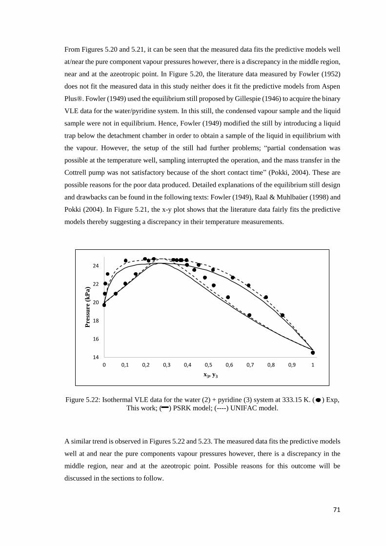
71

From Figures 5.20 and 5.21, it can be seen that the measured data fits the predictive models well

at/near the pure component vapour pressures however, there is a discrepancy in the middle region,

near and at the azeotropic point. In Figure 5.20, the literature data measured by Fowler (1952)

does not fit the measured data in this study neither does it fit the predictive models from Aspen

Plus®. Fowler (1949) used the equilibrium still proposed by Gillespie (1946) to acquire the binary

VLE data for the water/pyridine system. In this still, the condensed vapour sample and the liquid

sample were not in equilibrium. Hence, Fowler (1949) modified the still by introducing a liquid

trap below the detachment chamber in order to obtain a sample of the liquid in equilibrium with

the vapour. However, the setup of the still had further problems; “partial condensation was

possible at the temperature well, sampling interrupted the operation, and the mass transfer in the

Cottrell pump was not satisfactory because of the short contact time” (Pokki, 2004). These are

possible reasons for the poor data produced. Detailed explanations of the equilibrium still design

and drawbacks can be found in the following texts: Fowler (1949), Raal & Muhlbaüer (1998) and

Pokki (2004). In Figure 5.21, the x-y plot shows that the literature data fairly fits the predictive

models thereby suggesting a discrepancy in their temperature measurements.

Figure 5.22: Isothermal VLE data for the water (2) + pyridine (3) system at 333.15 K. ( ) Exp,


A similar trend is observed in Figures 5.22 and 5.23. The measured data fits the predictive models

well at and near the pure components vapour pressures however, there is a discrepancy in the

middle region, near and at the azeotropic point. Possible reasons for this outcome will be

discussed in the sections to follow.

14

16

18

20

22

24

0 0,1 0,2 0,3 0,4 0,5 0,6 0,7 0,8 0,9 1

Pre

ssu

re (

kP

a)

x3, y3

72

Figure 5.23: Isothermal x-y data for the water (2) + pyridine (3) system at 333.15 K. ( ) Exp,


Water (2) + Pyridine (3) System: Comparison of Experimental Data to Modelled Data

Figures 5.24 to 5.27 displays the isobaric and isothermal VLE data for the binary system of water

(2) + pyridine (3) at 40 kPa and 333.15 K respectively. The experimental measurements are

compared to the modelled data from Aspen Plus®.

Figure 5.24: Isobaric VLE data for the water (2) + pyridine (3) system at 40 kPa. ( ) Exp, This


UNIQUAC model.

0

0,1

0,2

0,3

0,4

0,5

0,6

0,7

0,8

0,9

1

0 0,1 0,2 0,3 0,4 0,5 0,6 0,7 0,8 0,9 1

y3

x3

342

344

346

348

350

352

354

356

358

360

0 0,1 0,2 0,3 0,4 0,5 0,6 0,7 0,8 0,9 1

Tem

per

atu

re (

K)

x3, y3

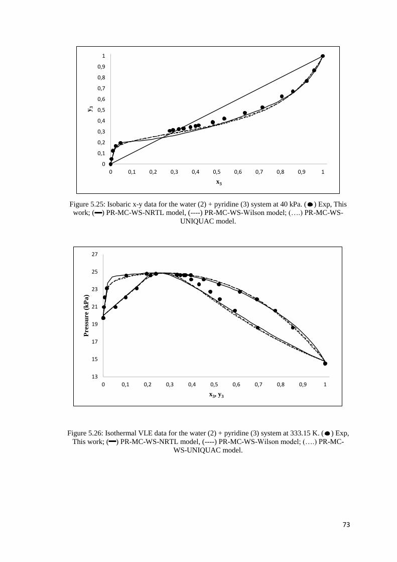
73

Figure 5.25: Isobaric x-y data for the water (2) + pyridine (3) system at 40 kPa. ( ) Exp, This


UNIQUAC model.

Figure 5.26: Isothermal VLE data for the water (2) + pyridine (3) system at 333.15 K. ( ) Exp,


WS-UNIQUAC model.

0

0,1

0,2

0,3

0,4

0,5

0,6

0,7

0,8

0,9

1

0 0,1 0,2 0,3 0,4 0,5 0,6 0,7 0,8 0,9 1

y3

x3

13

15

17

19

21

23

25

27

0 0,1 0,2 0,3 0,4 0,5 0,6 0,7 0,8 0,9 1

Pre

ssu

re (

kP

a)

x3, y3

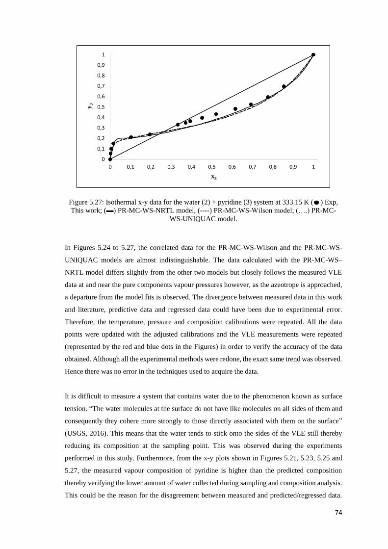
74

Figure 5.27: Isothermal x-y data for the water (2) + pyridine (3) system at 333.15 K ( ) Exp,


WS-UNIQUAC model.

In Figures 5.24 to 5.27, the correlated data for the PR-MC-WS-Wilson and the PR-MC-WS-

UNIQUAC models are almost indistinguishable. The data calculated with the PR-MC-WS–

NRTL model differs slightly from the other two models but closely follows the measured VLE

data at and near the pure components vapour pressures however, as the azeotrope is approached,

a departure from the model fits is observed. The divergence between measured data in this work

and literature, predictive data and regressed data could have been due to experimental error.

Therefore, the temperature, pressure and composition calibrations were repeated. All the data

points were updated with the adjusted calibrations and the VLE measurements were repeated

(represented by the red and blue dots in the Figures) in order to verify the accuracy of the data

obtained. Although all the experimental methods were redone, the exact same trend was observed.

Hence there was no error in the techniques used to acquire the data.

It is difficult to measure a system that contains water due to the phenomenon known as surface

tension. “The water molecules at the surface do not have like molecules on all sides of them and

consequently they cohere more strongly to those directly associated with them on the surface”

(USGS, 2016). This means that the water tends to stick onto the sides of the VLE still thereby

reducing its composition at the sampling point. This was observed during the experiments

performed in this study. Furthermore, from the x-y plots shown in Figures 5.21, 5.23, 5.25 and

5.27, the measured vapour composition of pyridine is higher than the predicted composition

thereby verifying the lower amount of water collected during sampling and composition analysis.

This could be the reason for the disagreement between measured and predicted/regressed data.

0

0,1

0,2

0,3

0,4

0,5

0,6

0,7

0,8

0,9

1

0 0,1 0,2 0,3 0,4 0,5 0,6 0,7 0,8 0,9 1

y3

x3

75

However, in this work, the water/pyridine feed composition (in the separation process) lies in the

water-rich region displayed on the graphs. It can be seen that a good correlation between the

experimental and modelled data is observed in this region, hence, the phase behaviour predicted

and separation process designed for the water/pyridine feed composition in this work will provide

an accurate representation of the real system.

Table 5.18 presents the azeotropic data for the water (2) + pyridine (3) system. Reported are the

azeotropic compositions observed in this work, literature, from predictive models and regressed

models from Aspen Plus®. It can be seen that the azeotropic composition in this study has a

greater pyridine composition than the sources to which it is compared. A possible reason for the

discrepancy is the surface tension phenomenon.

Table 5.18: Azeotropic data for the water (2) + pyridine (3) system

System Model x3 y3 T (K) P (kPa)

40 kPa

Experimental 0.321 0.323 344.5

Literature 0.258 0.232 343.3

PSRK 0.255 0.256 344.5

UNIFAC 0.255 0.264 343.9

PR-MC-WS-NRTL 0.255 0.250 343.8

PR-MC-WS-Wilson 0.275 0.280 343.5

PR-MC-WS-UNIQUAC 0.275 0.278 343.6

333.15 K

Experimental 0.333 0.331 24.67

PSRK 0.275 0.278 25.30

UNIFAC 0.275 0.276 24.93

PR-MC-WS-NRTL 0.255 0.249 24.88

PR-MC-WS-Wilson 0.255 0.261 24.88

PR-MC-WS-UNIQUAC 0.255 0.262 24.84

Tables 5.19 and 5.20 list the measured VLE data as well the deviation between temperature or

pressure and vapour compositions between experimental data and modelled data for each data

point, while Tables 5.21 and 5.22 list the AADs and AARDs for each system averaged over all

data points. The total AARD in each table represents the combined AARDs for temperature or

pressure and vapour compositions. Table 5.23 lists the regressed model parameters for each

system.

76

Table 5.19: Comparison of the experimental VLE data to modelled data for the water (2) + pyridine (3) system at 40 kPa

T (K) x3 y3 ∆Ta (K) ∆T/Ta (%) ∆y3a ∆y3/y3

a (%) ∆Tb (K) ∆T/Tb (%) ∆y3

b ∆y3/y3b

(%) ∆Tc (K) ∆T/Tc (%) ∆y3c ∆y3/y3

c (%)

347.74 0.004 0.048 0.1 0.02 0.005 10.75 0.1 0.03 0.007 15.10 0.1 0.04 0.008 16.77

346.04 0.010 0.123 0.4 0.12 0.018 14.44 0.5 0.14 0.022 18.17 0.4 0.12 0.020 15.91

345.05 0.023 0.169 0.0 0.01 0.007 4.42 0.4 0.13 0.025 14.55 0.3 0.10 0.021 12.32

344.45 0.046 0.196 0.2 0.04 0.002 0.80 0.3 0.09 0.019 9.85 0.2 0.08 0.018 9.33

343.87 0.279 0.309 0.1 0.03 0.050 16.28 0.4 0.12 0.026 8.59 0.4 0.11 0.029 9.52

343.92 0.294 0.316 0.2 0.04 0.052 16.43 0.5 0.13 0.028 8.99 0.4 0.12 0.032 10.04

343.90 0.321 0.323 0.1 0.02 0.049 15.05 0.4 0.12 0.026 8.06 0.4 0.11 0.030 9.33

343.98 0.342 0.329 0.1 0.03 0.046 13.86 0.5 0.13 0.024 7.33 0.4 0.13 0.029 8.77

343.77 0.344 0.330 0.1 0.04 0.045 13.69 0.3 0.07 0.024 7.20 0.2 0.06 0.029 8.66

343.87 0.376 0.342 0.1 0.04 0.043 12.65 0.3 0.08 0.024 7.07 0.3 0.07 0.030 8.76

344.05 0.400 0.353 0.1 0.02 0.043 12.14 0.4 0.11 0.026 7.34 0.4 0.10 0.032 9.16

343.92 0.415 0.359 0.3 0.08 0.041 11.52 0.2 0.06 0.026 7.21 0.2 0.05 0.033 9.10

344.53 0.481 0.389 0.1 0.03 0.036 9.23 0.5 0.14 0.028 7.19 0.4 0.13 0.036 9.26

344.39 0.482 0.386 0.2 0.07 0.033 8.51 0.3 0.10 0.025 6.48 0.3 0.09 0.033 8.57

345.07 0.535 0.422 0.0 0.01 0.037 8.82 0.7 0.18 0.036 8.57 0.6 0.17 0.045 10.58

346.33 0.632 0.474 0.1 0.03 0.025 5.32 0.9 0.25 0.036 7.57 0.8 0.23 0.043 9.12

347.53 0.715 0.525 0.1 0.02 0.013 2.42 0.7 0.20 0.029 5.56 0.6 0.17 0.034 6.43

350.07 0.807 0.626 0.7 0.20 0.028 4.54 0.9 0.27 0.041 6.52 0.8 0.23 0.042 6.63

351.25 0.859 0.672 0.4 0.12 0.012 1.76 0.3 0.08 0.014 2.15 0.2 0.05 0.014 2.08

353.84 0.924 0.769 0.5 0.13 0.003 0.38 0.2 0.06 0.013 1.62 0.2 0.06 0.012 1.53

356.20 0.959 0.866 0.8 0.23 0.016 1.80 0.1 0.03 0.005 0.58 0.2 0.04 0.003 0.36

∆𝑇 = |𝑇𝑒𝑥𝑝 − 𝑇𝑐𝑎𝑙𝑐| ∆𝑦2/𝑦2 = 100 |𝑦2𝑒𝑥𝑝− 𝑦2𝑐𝑎𝑙𝑐

𝑦2𝑒𝑥𝑝| cPR-MC-WS-UNIQUAC model

∆𝑦2 = |𝑦2𝑒𝑥𝑝 − 𝑦2𝑐𝑎𝑙𝑐| aPR-MC-WS-NRTL model

∆𝑇/T = 100 |𝑇𝑒𝑥𝑝− 𝑇𝑐𝑎𝑙𝑐

𝑇𝑒𝑥𝑝| bPR-MC-WS-Wilson model

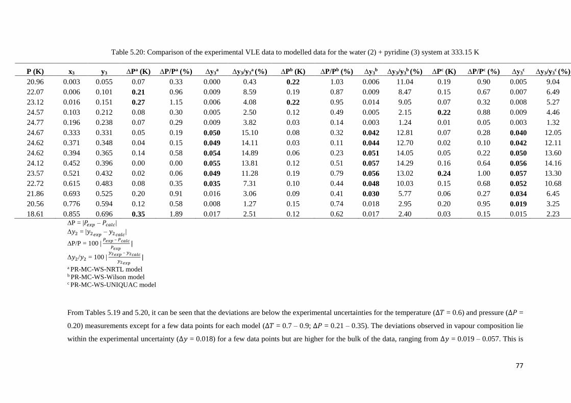
77

Table 5.20: Comparison of the experimental VLE data to modelled data for the water (2) + pyridine (3) system at 333.15 K

P (K) x3 y3 ∆Pa (K) ∆P/Pa (%) ∆y3a ∆y3/y3

a (%) ∆Pb (K) ∆P/Pb (%) ∆y3

b ∆y3/y3b

(%) ∆Pc (K) ∆P/Pc (%) ∆y3c ∆y3/y3

c (%)

20.96 0.003 0.055 0.07 0.33 0.000 0.43 0.22 1.03 0.006 11.04 0.19 0.90 0.005 9.04

22.07 0.006 0.101 0.21 0.96 0.009 8.59 0.19 0.87 0.009 8.47 0.15 0.67 0.007 6.49

23.12 0.016 0.151 0.27 1.15 0.006 4.08 0.22 0.95 0.014 9.05 0.07 0.32 0.008 5.27

24.57 0.103 0.212 0.08 0.30 0.005 2.50 0.12 0.49 0.005 2.15 0.22 0.88 0.009 4.46

24.77 0.196 0.238 0.07 0.29 0.009 3.82 0.03 0.14 0.003 1.24 0.01 0.05 0.003 1.32

24.67 0.333 0.331 0.05 0.19 0.050 15.10 0.08 0.32 0.042 12.81 0.07 0.28 0.040 12.05

24.62 0.371 0.348 0.04 0.15 0.049 14.11 0.03 0.11 0.044 12.70 0.02 0.10 0.042 12.11

24.62 0.394 0.365 0.14 0.58 0.054 14.89 0.06 0.23 0.051 14.05 0.05 0.22 0.050 13.60

24.12 0.452 0.396 0.00 0.00 0.055 13.81 0.12 0.51 0.057 14.29 0.16 0.64 0.056 14.16

23.57 0.521 0.432 0.02 0.06 0.049 11.28 0.19 0.79 0.056 13.02 0.24 1.00 0.057 13.30

22.72 0.615 0.483 0.08 0.35 0.035 7.31 0.10 0.44 0.048 10.03 0.15 0.68 0.052 10.68

21.86 0.693 0.525 0.20 0.91 0.016 3.06 0.09 0.41 0.030 5.77 0.06 0.27 0.034 6.45

20.56 0.776 0.594 0.12 0.58 0.008 1.27 0.15 0.74 0.018 2.95 0.20 0.95 0.019 3.25

18.61 0.855 0.696 0.35 1.89 0.017 2.51 0.12 0.62 0.017 2.40 0.03 0.15 0.015 2.23

∆P = |𝑃𝑒𝑥𝑝 – 𝑃𝑐𝑎𝑙𝑐 |


∆P/P = 100 | 𝑃𝑒𝑥𝑝 – 𝑃𝑐𝑎𝑙𝑐

𝑃𝑒𝑥𝑝 |

∆𝑦2/𝑦2 = 100 | 𝑦2𝑒𝑥𝑝 – 𝑦2𝑐𝑎𝑙𝑐

𝑦2𝑒𝑥𝑝 |


From Tables 5.19 and 5.20, it can be seen that the deviations are below the experimental uncertainties for the temperature (∆𝑇 = 0.6) and pressure (∆𝑃 =

0.20) measurements except for a few data points for each model (∆𝑇 = 0.7 – 0.9; ∆𝑃 = 0.21 – 0.35). The deviations observed in vapour composition lie

within the experimental uncertainty (∆𝑦 = 0.018) for a few data points but are higher for the bulk of the data, ranging from ∆𝑦 = 0.019 – 0.057. This is

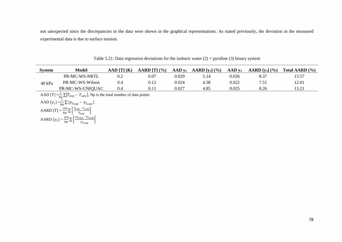
78

not unexpected since the discrepancies in the data were shown in the graphical representations. As stated previously, the deviation in the measured

experimental data is due to surface tension.

Table 5.21: Data regression deviations for the isobaric water (2) + pyridine (3) binary system

System Model AAD [T] (K) AARD [T] (%) AAD y2 AARD [y2] (%) AAD y3 AARD [y3] (%) Total AARD (%)

40 kPa

PR-MC-WS-NRTL 0.2 0.07 0.029 5.14 0.026 8.37 13.57

PR-MC-WS-Wilson 0.4 0.12 0.024 4.38 0.022 7.51 12.01

PR-MC-WS-UNIQUAC 0.4 0.11 0.027 4.85 0.025 8.26 13.21

AAD [T] =1

𝑁𝑝∑|𝑇𝑒𝑥𝑝 – 𝑇𝑐𝑎𝑙𝑐|, Np is the total number of data points

AAD [𝑦1] =1


AARD [T] = 100

𝑁𝑝∑ |

𝑇𝑒𝑥𝑝 – 𝑇𝑐𝑎𝑙𝑐

𝑇𝑒𝑥𝑝 |

AARD [𝑦1] = 100

𝑁𝑝∑ |


𝑦2𝑒𝑥𝑝 |

79

Table 5.22: Data regression deviations for the isothermal water (2) + pyridine (3) binary system.

System Model AAD [P] (kPa) AARD [P] (%) AAD y2 AARD [y2] (%) AAD y3 AARD [y3] (%) Total AARD (%)

333.15 K

PR-MC-WS-NRTL 0.14 0.65 0.026 4.48 0.023 6.87 12.00

PR-MC-WS-Wilson 0.14 0.65 0.028 5.01 0.025 7.96 13.62

PR-MC-WS-UNIQUAC 0.13 0.62 0.028 5.02 0.025 7.59 13.23

AAD [P] =1

𝑁𝑝∑|𝑃𝑒𝑥𝑝 – 𝑃𝑐𝑎𝑙𝑐|, Np is the total number of data points

AAD [𝑦1] =1


AARD [P] = 100

𝑁𝑝∑ |

𝑃𝑒𝑥𝑝 – 𝑃𝑐𝑎𝑙𝑐

𝑃𝑒𝑥𝑝 |

AARD [𝑦1] = 100

𝑁𝑝∑ |


𝑦2𝑒𝑥𝑝 |

From Tables 5.21 and 5.22, it can be seen that the thermodynamic model with the lowest deviation is the PR-MC-WS–NRTL for the 333.15 K system

(AARD = 12 %), hence the model parameters calculated with the use of this combination (presented in Table 5.23) were selected for the water (2) +

pyridine (3) system.

80

Table 5.23: Model parameters regressed for the water (2) + pyridine (3) binary system

System Model kija aijb ajib bijb bjib αijb RMSEc

40 kPa

PR-MC-WS-NRTL 0.37 996.40 419.40 0.69 11.67

PR-MC-WS-Wilson 0.22 8.40 13.49 -3178.64 -6044.71 11.32

PR-MC-WS-UNIQUAC -0.72 -853.65 -374.96 10.94

333.15 K

PR-MC-WS-NRTL 0.37 1052.13 345.52 0.69 13.46

PR-MC-WS-Wilson 0.25 -75.60 148.35 25063.29 -50872.47 14.33

PR-MC-WS-UNIQUAC -0.75 -891.38 -300.07 12.70 a WS mixing rule parameter incorporated into the PR EoS b NRTL/Wilson/UNIQUAC model parameters c RMSE: Residual mean square error

Ethanol (1) + Water (2) Binary System

The ethanol (1) + water (2) system was not measured since there is a wide range of consistent VLE data available for this system. Aspen Plus® stores

physical property parameters for several components in numerous databanks which are developed from the thermodynamic models available and data

from the Dortmund Databank. Hence the built-in parameters from Aspen Plus® for the ethanol (1) + water (2) system was used for the design.

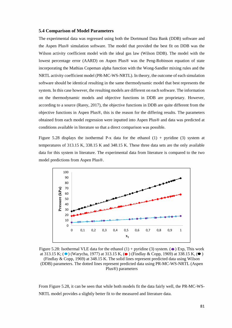
81

5.4 Comparison of Model Parameters

The experimental data was regressed using both the Dortmund Data Bank (DDB) software and

the Aspen Plus® simulation software. The model that provided the best fit on DDB was the

Wilson activity coefficient model with the ideal gas law (Wilson DDB). The model with the

lowest percentage error (AARD) on Aspen Plus® was the Peng-Robinson equation of state


NRTL activity coefficient model (PR-MC-WS-NRTL). In theory, the outcome of each simulation

software should be identical resulting in the same thermodynamic model that best represents the

system. In this case however, the resulting models are different on each software. The information

on the thermodynamic models and objective functions in DDB are proprietary. However,

according to a source (Rarey, 2017), the objective functions in DDB are quite different from the

objective functions in Aspen Plus®, this is the reason for the differing results. The parameters

obtained from each model regression were inputted into Aspen Plus® and data was predicted at

conditions available in literature so that a direct comparison was possible.

Figure 5.28 displays the isothermal P-x data for the ethanol (1) + pyridine (3) system at

temperatures of 313.15 K, 338.15 K and 348.15 K. These three data sets are the only available

data for this system in literature. The experimental data from literature is compared to the two

model predictions from Aspen Plus®.

Figure 5.28: Isothermal VLE data for the ethanol (1) + pyridine (3) system. ( ) Exp, This work

at 313.15 K; ( ) (Warycha, 1977) at 313.15 K, ( ) (Findlay & Copp, 1969) at 338.15 K, ( )

(Findlay & Copp, 1969) at 348.15 K. The solid lines represent predicted data using Wilson

(DDB) parameters. The dotted lines represent predicted data using PR-MC-WS-NRTL (Aspen

Plus®) parameters

From Figure 5.28, it can be seen that while both models fit the data fairly well, the PR-MC-WS-

NRTL model provides a slightly better fit to the measured and literature data.

0

10

20

30

40

50

60

70

80

90

100

0 0,1 0,2 0,3 0,4 0,5 0,6 0,7 0,8 0,9 1

Pre

ssu

re (

kP

a)

x1

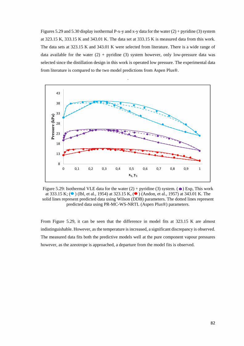
82

Figures 5.29 and 5.30 display isothermal P-x-y and x-y data for the water (2) + pyridine (3) system

at 323.15 K, 333.15 K and 343.01 K. The data set at 333.15 K is measured data from this work.

The data sets at 323.15 K and 343.01 K were selected from literature. There is a wide range of

data available for the water (2) + pyridine (3) system however, only low-pressure data was

selected since the distillation design in this work is operated low pressure. The experimental data

from literature is compared to the two model predictions from Aspen Plus®.

.

Figure 5.29: Isothermal VLE data for the water (2) + pyridine (3) system. ( ) Exp, This work

at 333.15 K; ( ) (Ibl, et al., 1954) at 323.15 K, ( ) (Andon, et al., 1957) at 343.01 K. The

solid lines represent predicted data using Wilson (DDB) parameters. The dotted lines represent

predicted data using PR-MC-WS-NRTL (Aspen Plus®) parameters.

From Figure 5.29, it can be seen that the difference in model fits at 323.15 K are almost

indistinguishable. However, as the temperature is increased, a significant discrepancy is observed.

The measured data fits both the predictive models well at the pure component vapour pressures

however, as the azeotrope is approached, a departure from the model fits is observed.

8

13

18

23

28

33

38

43

0 0,1 0,2 0,3 0,4 0,5 0,6 0,7 0,8 0,9 1

Pre

ssu

re (

kP

a)

x3, y3

83

Figure 5.30: Isothermal x-y data for the water (2) + pyridine (3) system. ( ) Exp, This work at

333.15 K; ( ) (Ibl, et al., 1954) at 323.15 K, ( ) (Andon, et al., 1957) at 343.01 K. The solid

lines represent predicted data using Wilson (DDB) parameters. The dotted lines represent

predicted data using PR-MC-WS-NRTL (Aspen Plus®) parameters.

Similarly, in Figure 5.30, there is a deviation between the measured data from this work and the

trend predicted with the selected model parameters, as the azeotropic composition is approached.

Additionally, it can be seen that the measured data in the middle region lies closer to the

equilibrium line resulting in a relative volatility (𝛼) closer to 1. For example, at x = 0.5,

experimental 𝛼 = 1.38, Wilson DDB 𝛼 = 1.70 and PR-MC-WS-NRTL 𝛼 = 1.77. The closer the

relative volatility is to 1, the greater the number of theoretical stages required for the separation

process. Since the thermodynamic models predict a relative volatility further away from 1, the

theoretical stages calculated in the simulation will be lower than what is required for the real

system. However, the efficiency introduced into the column design will account for this

discrepancy. Nonetheless, as discussed in previous sections, the water/pyridine feed composition

in this work lies in the water-rich region. As seen from the Figure, there is a good correlation

between the experimental and modelled data in this region. Hence, the phase behaviour predicted

and separation process designed in this region will provide an accurate representation of the real

system.

Table 5.24 presents the AADs for each system averaged over all data points. From the Table, it

can be seen that the AADs are lower for the PR-MC-WS-NRTL model. Hence, this model

combination better represents the measured data.

0

0,1

0,2

0,3

0,4

0,5

0,6

0,7

0,8

0,9

1

0 0,1 0,2 0,3 0,4 0,5 0,6 0,7 0,8 0,9 1

y3

x3

84

Table 5.24: Data regression deviations for the systems studied averaged over all points.

System Model AAD [T] (K) AAD [P] (kPa) AAD y1 AAD y3

EP 40 kPa Wilson DDB 0.4 0.005 PR-MC-WS-NRTL 0.2 0.004

EP 100 kPa Wilson DDB 0.3 0.026 PR-MC-WS-NRTL 0.3 0.017

EP 313.15 K Wilson DDB 0.24 0.008 PR-MC-WS-NRTL 0.01 0.005

WP 40 kPa Wilson DDB 0.3 0.027

PR-MC-WS-NRTL 0.2 0.026

WP 333.15 K Wilson DDB 0.28 0.031

PR-MC-WS-NRTL 0.14 0.025

EP: Ethanol (1) + Pyridine (3) WP: Water (2) + Pyridine (3)

85

CHAPTER 6: PROCESS DESIGN AND COSTING

6.1 Design Methodology

In this study, process design via a simulative approach is used to represent the behaviour of a

chemical process. This is based on the information and thermodynamic models in the design

methods of the simulation software. The objective of process design in this study was to develop

and simulate a process (with the use of the Aspen Plus® process simulator) to efficiently separate

and recover the waste material comprising pyridine, ethanol, water and nitrogen with recovery

rates and mole purities greater than 99.9 % so that the components could be recycled and reused

in the LiPF6 production process.

Two separation schemes were investigated. The first proposed process (process A) comprises a

flash vessel to remove the nitrogen, a conventional distillation column to separate the pyridine

from the mixture followed by an extractive distillation column to separate the ethanol from water.

As discussed in section 2.3, the solvent chosen for extractive distillation was ethylene glycol. This

was recovered in a solvent recovery distillation column and recycled to the extractive distillation

column for reuse. This recycle loop was closed and the process converged with the use of a

calculator block. In Aspen Plus®, a calculator is used to insert FORTRAN code into the

simulation. FORTRAN is a programming language widely used for scientific calculations.

Converging a process simulation that contains a recycle loop is not easy, hence the calculator was

used to determine the amount of make-up solvent required to balance all component flow rates

within the process.

The second process (process B) follows the same scheme as process A for the nitrogen and

pyridine separation; however, it uses a pervaporation unit to separate ethanol from water as

opposed to the extractive distillation column in process A. A polyvinylalcohol membrane in a

spiral wound module configuration was selected as discussed in section 2.4. In this case, the

retentate stream comprises the high purity ethanol product; the permeate stream comprises a

mixture of ethanol and water. This permeate stream is recycled to the conventional distillation

column to prevent the loss of ethanol.

A modification was made to each process where an additional flash vessel was used to further

purify the nitrogen stream. However, the viability of this additional flash vessel had to be

determined. Therefore, the processes were optimised and a cost evaluation performed to

determine how the second flash would affect the total cost and final purities. In the sections to

follow, process A will be referred to as process 1FE (1-flash extractive), process B will be referred

to process 1FM (1-flash membrane), the modification to process A will be process 2FE (2-flash

extractive) and the modification to process B will be process 2FM (2-flash membrane).

86

NoS: 73

RR: 0.495

QC: 8.04 MW

QR: 9.22 MW

NoS: 50

RR: 0.6

S/F: 2.2

QC: 7.51 MW

QR: 12.89 MW

NoS: 33

RR: 2.47

QC: 3.07 MW

QR: 2.48 MW

Q: 275.21 kW

Q: 21.38 kW

Figure 6.1: Process A

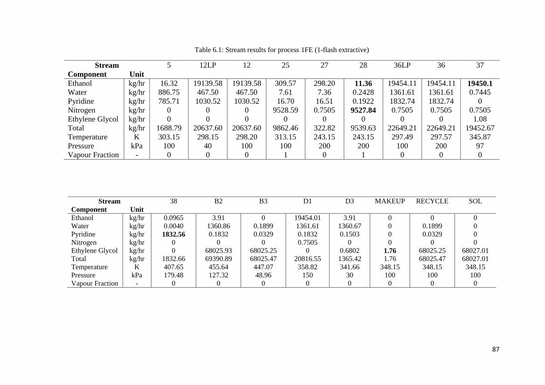
87

Table 6.1: Stream results for process 1FE (1-flash extractive)

Stream 5 12LP 12 25 27 28 36LP 36 37

Component Unit

Ethanol kg/hr 16.32 19139.58 19139.58 309.57 298.20 11.36 19454.11 19454.11 19450.1

Water kg/hr 886.75 467.50 467.50 7.61 7.36 0.2428 1361.61 1361.61 0.7445

Pyridine kg/hr 785.71 1030.52 1030.52 16.70 16.51 0.1922 1832.74 1832.74 0

Nitrogen kg/hr 0 0 0 9528.59 0.7505 9527.84 0.7505 0.7505 0.7505

Ethylene Glycol kg/hr 0 0 0 0 0 0 0 0 1.08

Total kg/hr 1688.79 20637.60 20637.60 9862.46 322.82 9539.63 22649.21 22649.21 19452.67

Temperature K 303.15 298.15 298.20 313.15 243.15 243.15 297.49 297.57 345.87

Pressure kPa 100 40 100 100 200 200 100 200 97

Vapour Fraction - 0 0 0 1 0 1 0 0 0

Stream 38 B2 B3 D1 D3 MAKEUP RECYCLE SOL

Component Unit

Ethanol kg/hr 0.0965 3.91 0 19454.01 3.91 0 0 0

Water kg/hr 0.0040 1360.86 0.1899 1361.61 1360.67 0 0.1899 0

Pyridine kg/hr 1832.56 0.1832 0.0329 0.1832 0.1503 0 0.0329 0

Nitrogen kg/hr 0 0 0 0.7505 0 0 0 0

Ethylene Glycol kg/hr 0 68025.93 68025.25 0 0.6802 1.76 68025.25 68027.01

Total kg/hr 1832.66 69390.89 68025.47 20816.55 1365.42 1.76 68025.47 68027.01

Temperature K 407.65 455.64 447.07 358.82 341.66 348.15 348.15 348.15

Pressure kPa 179.48 127.32 48.96 150 30 100 100 100

Vapour Fraction - 0 0 0 0 0 0 0 0

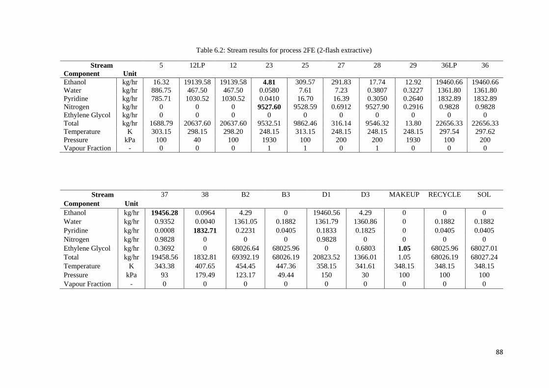
88

Table 6.2: Stream results for process 2FE (2-flash extractive)

Stream 5 12LP 12 23 25 27 28 29 36LP 36

Component Unit

Ethanol kg/hr 16.32 19139.58 19139.58 4.81 309.57 291.83 17.74 12.92 19460.66 19460.66

Water kg/hr 886.75 467.50 467.50 0.0580 7.61 7.23 0.3807 0.3227 1361.80 1361.80

Pyridine kg/hr 785.71 1030.52 1030.52 0.0410 16.70 16.39 0.3050 0.2640 1832.89 1832.89

Nitrogen kg/hr 0 0 0 9527.60 9528.59 0.6912 9527.90 0.2916 0.9828 0.9828

Ethylene Glycol kg/hr 0 0 0 0 0 0 0 0 0 0

Total kg/hr 1688.79 20637.60 20637.60 9532.51 9862.46 316.14 9546.32 13.80 22656.33 22656.33

Temperature K 303.15 298.15 298.20 248.15 313.15 248.15 248.15 248.15 297.54 297.62

Pressure kPa 100 40 100 1930 100 200 200 1930 100 200

Vapour Fraction - 0 0 0 1 1 0 1 0 0 0

Stream 37 38 B2 B3 D1 D3 MAKEUP RECYCLE SOL

Component Unit

Ethanol kg/hr 19456.28 0.0964 4.29 0 19460.56 4.29 0 0 0

Water kg/hr 0.9352 0.0040 1361.05 0.1882 1361.79 1360.86 0 0.1882 0.1882

Pyridine kg/hr 0.0008 1832.71 0.2231 0.0405 0.1833 0.1825 0 0.0405 0.0405

Nitrogen kg/hr 0.9828 0 0 0 0.9828 0 0 0 0

Ethylene Glycol kg/hr 0.3692 0 68026.64 68025.96 0 0.6803 1.05 68025.96 68027.01

Total kg/hr 19458.56 1832.81 69392.19 68026.19 20823.52 1366.01 1.05 68026.19 68027.24

Temperature K 343.38 407.65 454.45 447.36 358.15 341.61 348.15 348.15 348.15

Pressure kPa 93 179.49 123.17 49.44 150 30 100 100 100

Vapour Fraction - 0 0 0 0 0 0 0 0 0

89

Process A

Process A is presented in Figure 6.1 while the flow rates and operating conditions for each stream are

shown in Table 6.1 for process 1FE (1-flash extractive) and 6.2 for process 2FE (2-flash extractive). The

waste streams that require purification and recycling from the LiPF6 production process are stream 25

(comprising nitrogen, ethanol, water and pyridine at 313.15 K and 100 kPa), stream 5 (comprising

ethanol, water and pyridine at 303.15 K and 100 kPa) and stream 12 (comprising ethanol, water and

pyridine at 298.15 K and 40 kPa). Stream 25 is first fed into flash vessel F-01 which operates at a

temperature and pressure of 243.15 K and 200 kPa respectively. Stream 28 exits the top of F-01 and is

fed to flash vessel F-02 which is operated at a temperature and pressure of 248.15 K and 1930 kPa

respectively. Nitrogen with a recovery of 99.99 mol % and a purity of 99.97 mol % exits the top of F-

02 (stream 23). The bottoms of F-01 (stream 27) and F-02 (stream 29) is then combined with streams

5 and 12 and fed to a conventional distillation column (C-01) with an operating pressure of 150 kPa.

Pyridine exits the bottom of the column (stream 38) with a recovery and purity of 99.99 mol %. The

distillate (stream D1) comprising the ethanol/water azeotrope is then fed to an extractive distillation

column (C-02) together with the ethylene glycol solvent (operating pressure of 97 kPa). Ethanol exits

in the distillate (stream 37) with a recovery and purity of 99.98 mol %. The bottoms (stream B2)

comprising water and ethylene glycol is then fed to a solvent recovery column (C-03) with an operating

pressure of 30 kPa. Ethylene glycol exits the bottom of the column with a recovery and purity of 99.99

mol % and is recycled to the extractive distillation column (C-02) for reuse. The recycle loop was closed

and the process converged with the use of a calculator block. The distillate (stream D3) comprises

mainly water and trace amounts of ethylene glycol. Therefore, a solvent make-up of 0.02 kmol/hr

(stream MAKEUP) is required to account for the loss of solvent to the water-rich stream D3. All the

purities and recovery rates are greater than 99.9 mol % and hence meet the required specifications as

proposed by NECSA.

The modification to process A is indicated by the additional flash vessel within the red dotted lines. As

seen in Table 6.1, the nitrogen-rich stream (stream 28) exiting the top of flash vessel F-01 still contains

11.36 kg/hr of ethanol. The purpose of the additional flash vessel was to reduce this ethanol thereby

further purifying the nitrogen stream. As seen in Table 6.2, the nitrogen rich stream (stream 23) exiting

the top of flash vessel F-02 contains 4.81 kg/hr of ethanol. Therefore, the additional flash vessel

recovered a further 6.55 kg/hr of ethanol. Furthermore, an additional 0.15 kg/hr of pyridine was

recovered in stream 37 and the solvent make-up required decreased by 0.71 kg/hr.

The column specifications shown in Figure 6.1 (number of stages, reflux ratio, duties, etc) are discussed

in section 6.2.

90

Figure 6.2: Process B

NoS: 63

RR: 0.465

QC: 9.99 MW

QR: 10.97 MW Q: 275.21 kW

Q: 21.38 kW

91

Table 6.3: Stream results for process 1FM (1-flash membrane)

Stream 5 12LP 12 25 27 28 36LP 36 38 D1 Retentate Permeate

Component Unit

Ethanol kg/hr 16.32 19139.6 19139.6 309.57 298.20 11.36 19454.1 19454.1 0.0965 19454.1 17650.09 1832.63

Water kg/hr 886.75 467.50 467.50 7.61 7.36 0.2428 1361.61 1361.61 0.0040 1361.61 14.45 1346.19

Pyridine kg/hr 785.71 1030.52 1030.52 16.70 16.51 0.1922 1832.74 1832.74 1832.56 0.1832 0 0

Nitrogen kg/hr 0 0 0 9528.59 0.7505 9527.84 0.7505 0.7505 0 0.7505 0 0

Ethylene Glycol kg/hr 0 0 0 0 0 0 0 0 0 0 0 0

Total kg/hr 1688.79 20637.6 20637.6 9862.46 322.82 9539.63 22649.2 22649.2 1832.66 20816.6 17664.54 3169.82

Temperature K 303.15 298.15 298.20 313.15 243.15 243.15 303.03 303.07 395.11 346.59 333.15 333.15

Pressure kPa 100 40 100 100 200 200 100 150 129.98 100 100 2.03

Vapour Fraction - 0 0 0 1 0 1 0 0 0 0 0 0

Table 6.4: Stream results for process 2FM (2-flash membrane)

Stream 5 12LP 12 23 25 27 28 29 36 38 D1 Retentate Permeate

Component Unit

Ethanol kg/hr 16.32 19139.6 19139.6 4.81 309.57 291.83 17.74 12.92 19460.7 0.0964 19460.6 17650.09 1823.63

Water kg/hr 886.75 467.50 467.50 0.0580 7.61 7.23 0.3807 0.3227 1361.80 0.0040 1361.79 14.45 1346.19

Pyridine kg/hr 785.71 1030.52 1030.52 0.0410 16.70 16.39 0.3050 0.2640 1832.89 1832.71 0.1833 0 0

Nitrogen kg/hr 0 0 0 9527.60 9528.59 0.6912 9527.90 0.2916 0.9828 0 0.9828 0 0

Ethylene Glycol kg/hr 0 0 0 0 0 0 0 0 0 0 0 0 0

Total kg/hr 1688.79 20637.6 20637.6 9532.51 9862.46 316.14 9546.32 13.80 22656.3 1832.81 20823.5 17664.54 3169.82

Temperature K 303.15 298.15 298.20 248.15 313.15 248.15 248.15 248.15 303.11 394.90 345.89 333.15 333.15

Pressure kPa 100 40 100 1930 100 200 200 1930 150 129.21 100 100 2.03

Vapour Fraction - 0 0 0 1 1 0 1 0 0 0 0 0 0

92

Process B

Process B is presented in Figure 6.2 while the flow rates and operating conditions for each stream are

shown in Table 6.3 for process 1FM (1-flash membrane) and 6.4 for process 2FM (2-flash membrane).

Stream 25 is first fed into flash vessel F-01 which operates at a temperature and pressure of 243.15 K

and 200 kPa respectively. Stream 28 exits the top of F-01 and is fed to flash vessel F-02 which is operated

at a temperature and pressure of 248.15 K and 1930 kPa respectively. Nitrogen with a recovery of 99.99

mol % and a purity of 99.97 mol % exits the top of F-02 (stream 23). The bottoms of F-01 (stream 27)

and F-02 (stream 29) is then combined with streams 5 and 12 and fed to a conventional distillation

column (C-01) with an operating pressure of 100 kPa. Pyridine exits the bottom of the column (stream

38) with a recovery and purity of 99.99 mol %. The distillate (stream D1) comprising the ethanol/water

azeotrope is then fed to a pervaporation unit where ethanol leaves in the retentate stream with a recovery

and purity of 90.64 mol % and 99.79 % respectively. The permeate stream (comprising water and the

remaining ethanol) is then recycled to the conventional distillation column (C-01) to prevent the loss of

ethanol.

The modification to process B is indicated by the additional flash vessel within the red dotted lines. As

seen from Tables 6.3 and 6.4, the use of the additional flash vessel results in the recovery increase for

ethanol and pyridine by 6.55 kg/hr and 0.15 kg/hr respectively, similarly to process A.

The column specifications shown in Figure 6.2 (number of stages, reflux ratio, duties, etc) are discussed

in section 6.2.

93

6.2 Process Optimisation

6.2.1 Flash Vessels

The first units to be optimised were the flash vessels. The purpose of these vessels were to separate

nitrogen from pyridine, ethanol and water. The vessel temperature and pressure were both varied

to maximise recovery of nitrogen in the vapour outlet and maximise recovery of ethanol, water

and pyridine in the liquid outlet. Pyridine and water separates easily from nitrogen; however

recovering the ethanol was more challenging. The results showed that as the temperature

decreased, the separation improved; however to avoid the use of a more expensive refrigerant and

higher cooling duty costs, the temperature selected was 243.15 K for processes 1FE & 1FM and

248.15 K for processes 2FE & 2FM. The material of construction selected was stainless steel due

to the low vessel temperature required for separation.

Figure 6.3 displays a plot of the nitrogen mole fraction, nitrogen mole recovery and ethanol mass

flow rate in the vapour outlet (stream 28) varied with the column pressure for flash vessel F-01

for processes 1FE & 1FM. It can be seen that as the nitrogen purity increases the ethanol flow

rate and nitrogen recovery decreases. The pressure selected should achieve a high nitrogen purity

and recovery whilst minimising the ethanol flow rate in the vapour outlet. A pressure of 200 kPa

was chosen since this is the point at which the curvature is most sharply changing. This results in

a nitrogen purity and recovery of 99.92 mol % and 99.99 mol % respectively, and 11.36 kg/hr of

ethanol in the vapour stream.

Figure 6.3: Influence of pressure on the nitrogen mole purity, nitrogen recovery and ethanol

mass flow rate in the vapour outlet for F-01 (1-flash process)

0

5

10

15

20

25

0,9984

0,9986

0,9988

0,9990

0,9992

0,9994

0,9996

0,9998

1,0000

100 150 200 250 300 350 400

Eth

ano

l M

ass

Flo

w (

kg/h

r)

Nit

rogen

Mo

le F

ract

ion

Pressure (kPa)

Nitrogen Purity Nitrogen Recovery Ethanol (kg/hr)

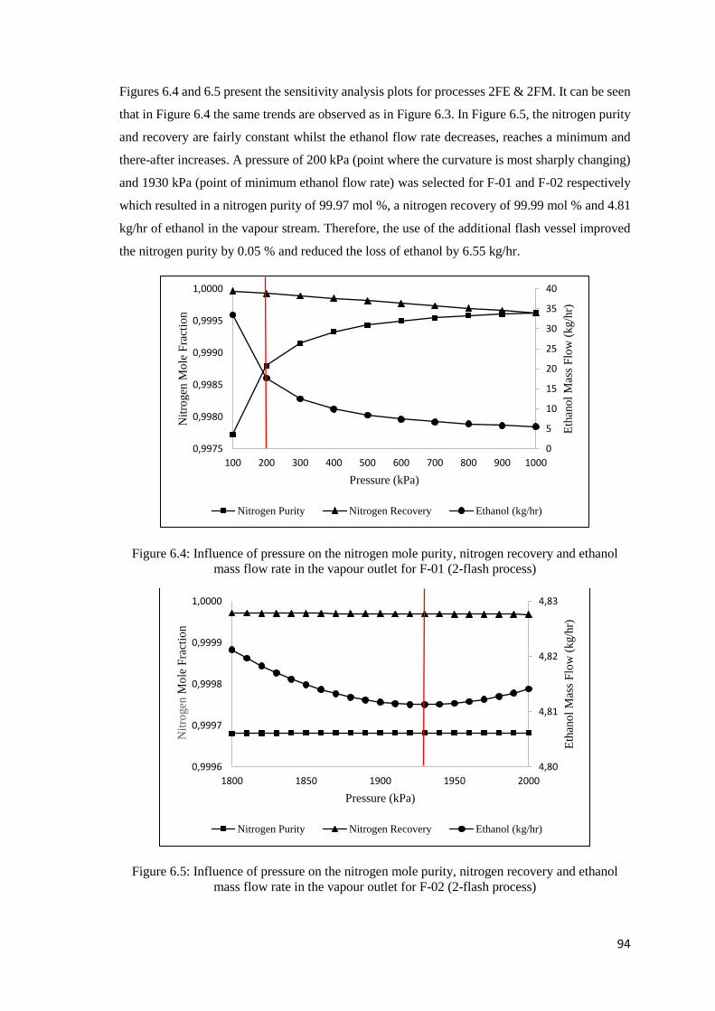
94

Figures 6.4 and 6.5 present the sensitivity analysis plots for processes 2FE & 2FM. It can be seen

that in Figure 6.4 the same trends are observed as in Figure 6.3. In Figure 6.5, the nitrogen purity

and recovery are fairly constant whilst the ethanol flow rate decreases, reaches a minimum and

there-after increases. A pressure of 200 kPa (point where the curvature is most sharply changing)

and 1930 kPa (point of minimum ethanol flow rate) was selected for F-01 and F-02 respectively

which resulted in a nitrogen purity of 99.97 mol %, a nitrogen recovery of 99.99 mol % and 4.81

kg/hr of ethanol in the vapour stream. Therefore, the use of the additional flash vessel improved

the nitrogen purity by 0.05 % and reduced the loss of ethanol by 6.55 kg/hr.





0

5

10

15

20

25

30

35

40

0,9975

0,9980

0,9985

0,9990

0,9995

1,0000

100 200 300 400 500 600 700 800 900 1000

Eth

ano

l M

ass

Flo

w (

kg/h

r)

Nit

rogen

Mo

le F

ract

ion

Pressure (kPa)


4,80

4,81

4,82

4,83

0,9996

0,9997

0,9998

0,9999

1,0000

1800 1850 1900 1950 2000

Eth

ano

l M

ass

Flo

w (

kg/h

r)

Nit

rogen

Mo

le F

ract

ion

Pressure (kPa)


95

6.3.2 Distillation Columns

The RadFrac model in Aspen Plus® was selected to simulate the distillation processes. RadFrac

is a rigorous model for simulating multi-stage vapour-liquid fractioning operations. RadFrac may

operate using either the traditional equilibrium-based approach (efficiency required to account for

deviations from equilibrium) or the rate-based method (able to simulate real tray behaviour). It is

more efficient to use the equilibrium-based method for column optimisation due to the longer

calculation times and higher likelihood of convergence problems in the rate-based method. Hence,

in this work, the total number of theoretical stages were calculated using an equilibrium-based

method. The rate-based method was then incorporated to back-calculate the Murphree efficiencies

of each component. These efficiencies were averaged over the entire column (Table 6.5) and were

there-after used to resize the column using the equilibrium-based method. Sieve trays were

specified due to their low cost, low pressure drop and high efficiency. The column material

selected was carbon steel since the operating conditions were not extreme (too high or too low

temperatures and pressures) and the components used in the process were not particularly

corrosive.

Table 6.5: Component Murphree Efficiencies

Components C-01 C-02 C-03

Ethanol 0.61 0.62 -

Water 0.65 0.67 0.65

Pyridine 0.63 0.67 -

Ethylene Glycol - - 0.65

Distillate or bottoms rate

For effective separation of species to occur in the distillation column, the distillate or bottoms

flow rate is specified. If the light key component was to be removed, the distillate rate was

specified. Similarly, if the heavy key component was to be removed, the bottoms rate was

specified. For example, for a mixture of ethanol, water and pyridine; it was desired to achieve a

separation with 99.8% mole composition of pyridine recovered as a product for reuse. Since

pyridine has the highest boiling point, it is the heavy key component. Thus, the bottoms rate was

selected, with a purity of 99.8% pyridine specified. The remaining 0.02% was sent to the distillate

along with majority of the ethanol and water.

Column Pressure

The effect of the column pressure depends on the system of components to be separated. A change

in the column pressure could possibly increase equipment or operating costs. However, in some

cases this change may be necessary to reach desired purities, prevent thermal degradation and

96

avoid the use of refrigeration or high heating requirements. It is ideal to operate the distillation

column at atmospheric pressure; however, it is not always possible. Table 6.6 present the critical

temperatures and pressures for the components of interest. The reboiler temperature and pressure

should not be close to or above these critical values so that vapour-liquid equilibrium is still

possible.

The columns were operated at/near atmospheric pressure resulting in high condenser and reboiler

temperatures of 341 – 359 K and 407 – 456 K respectively, due to the pyridine and ethylene glycol

present in the system. However, this pressure is required to enable the use of cooling water as the

condensing medium (reducing the pressure to vacuum operation requires chilled water).

Furthermore, the resulting reboiler temperatures and pressures were well below the critical values

and low enough such that thermal degradation did not occur at the specified column conditions.

A pressure drop 0.0068 atm was specified per tray as advised by Luyben (2013).

Table 6.6: Critical properties of components

TC (K) PC (MPa)

Ethanol 516.25a 6.39a

Water 647.10b 22.06b

Pyridine 620c 5.63c

Ethylene Glycol 720d 8.2d

a (Vesovic, 2011)

b (Chaplin, 2017)

c (PubChem, 2004)

d (MEGlobal, 2017)

This section presents the optimisation procedure for process A (1FE & 1FM). The remaining

processes followed a similar approach and are presented in Appendix E.

Conventional Distillation Column (C-01)

This design involved optimising the following variables: number of stages, feed stage location,

reflux ratio and the distillate or bottoms rate. Since the system of components are non-ideal and

each with a significant difference in boiling temperature, the simple heuristic design approach

(setting the total number of trays to twice the minimum or setting the reflux ratio to 1.3 times the

minimum) could not be utilised. Instead the rigorous method was implemented. This involved

varying the number of stages against the capital and operating costs and selecting the

configuration that gave the minimum total annual cost (TAC).

The total annual cost (TAC) is represented by the following equation:

𝑇𝐴𝐶 (𝑅 103

𝑦𝑒𝑎𝑟) = 𝐶𝑣 + 𝐶𝑓 + (𝑖𝑟 + 𝑖𝑚) × 𝐹𝐶 (6.1)

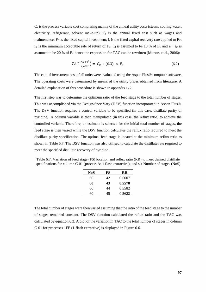
97

Cv is the process variable cost comprising mainly of the annual utility costs (steam, cooling water,

electricity, refrigerant, solvent make-up); Cf is the annual fixed cost such as wages and

maintenance; FC is the fixed capital investment; ir is the fixed capital recovery rate applied to FC;

im is the minimum acceptable rate of return of FC. Cf is assumed to be 10 % of FC and ir + im is

assumed to be 20 % of FC hence the expression for TAC can be rewritten (Munoz, et al., 2006):

𝑇𝐴𝐶 (𝑅 103

𝑦𝑒𝑎𝑟) = 𝐶𝑣 + (0.3) × 𝐹𝐶 (6.2)

The capital investment cost of all units were evaluated using the Aspen Plus® computer software.

The operating costs were determined by means of the utility prices obtained from literature. A

detailed explanation of this procedure is shown in appendix B.2.

The first step was to determine the optimum ratio of the feed stage to the total number of stages.

This was accomplished via the Design/Spec Vary (DSV) function incorporated in Aspen Plus®.

The DSV function requires a control variable to be specified (in this case, distillate purity of

pyridine). A column variable is then manipulated (in this case, the reflux ratio) to achieve the

controlled variable. Therefore, an estimate is selected for the initial total number of stages, the

feed stage is then varied while the DSV function calculates the reflux ratio required to meet the

distillate purity specification. The optimal feed stage is located at the minimum reflux ratio as

shown in Table 6.7. The DSV function was also utilised to calculate the distillate rate required to

meet the specified distillate recovery of pyridine.

Table 6.7: Variation of feed stage (FS) location and reflux ratio (RR) to meet desired distillate

specifications for column C-01 (process A: 1 flash extractive), and set Number of stages (NoS)

NoS FS RR

60 42 0.5607

60 43 0.5578

60 44 0.5582

60 45 0.5622

The total number of stages were then varied assuming that the ratio of the feed stage to the number

of stages remained constant. The DSV function calculated the reflux ratio and the TAC was

calculated by equation 6.2. A plot of the variation in TAC to the total number of stages in column

C-01 for processes 1FE (1-flash extractive) is displayed in Figure 6.6.

98

Figure 6.6: Influence of the number of stages on TAC for column C-01, process A: 1 flash

extractive

As seen from the Figure, the minimum TAC is located at 75 stages hence this was selected as the

optimal value. There-after, the feed stage was once again varied while the number of stages

remained constant at 75. The DSV function calculated the reflux ratio for each case. The TAC

was then calculated for each case and is displayed in Figure 6.7. The optimal feed stage is located

at stage 58 (minimum TAC) with a reflux ratio of 0.490.

Figure 6.7: Influence of the feed stage on the total annual cost at 75 stages for column C-01,

process A: 1 flash extractive

2,09E+06

2,10E+06

2,11E+06

2,12E+06

2,13E+06

2,14E+06

2,15E+06

2,16E+06

2,17E+06

2,18E+06

55 60 65 70 75 80

TA

C (

US

D)

Number of Stages

2,092E+06

2,094E+06

2,096E+06

2,098E+06

2,100E+06

2,102E+06

2,104E+06

2,106E+06

2,108E+06

52 53 54 55 56 57 58 59 60

TA

C (

US

D)

Feed Stage

99

Extractive Distillation Column (C-02)

The extractive distillation design is more complicated and a different approach is adopted as

compared to the conventional distillation column. In this case, the distillate purity and recovery

of ethanol was set to 99.98 mol %. The solvent to feed ratio was set to 2.0 initially (less than 2.0

does not meet the distillate specifications despite the number of stages). The number of stages

were varied selecting in each case the optimal feed stage, solvent feed stage and reflux ratio. The

reboiler heat duty (RHD) was recorded in each case and plotted against the number of stages as

shown in Figure 6.8.

Figure 6.8: Influence of number of stages on reboiler heat duty for column C-02, process A: 1

flash extractive

The 6 cases with the lowest RHD were selected for further investigation. As seen from the Figure,

this includes stages 50 (case 1), 51 (case 2), 52 (case 3), 54 (case 4), 55 (case 5) and 56 (case 6).

The variables (number of stages, feed stage, solvent feed stage and reflux ratio) for each case

were inputted into Aspen Plus® and there-after, the solvent to feed ratio was adjusted to minimise

the RHD in each case. Figure 6.9 shows this effect for case 5.

13,0

13,5

14,0

14,5

15,0

15,5

47 49 51 53 55 57

Reb

oil

er D

uty

(M

W)

Number of Stages

100

Figure 6.9: Effect of solvent to feed ratio on RHD for case 5 for column C-02, process A: 1

flash extractive

As seen in Figure 6.9, the optimal solvent to feed ratio was 2.2 as this is the value with the

minimum RHD. The same procedure was followed for the remaining cases. The results are

displayed in Table 6.8.

Table 6.8: Extractive distillation column specifications for each case for column C-02, process

A: 1 flash extractive

Case NoS FS SFS RR S/F Ratio Purity Recovery RHD (MW)

1 47 37 8 0.6 2.4 0.9998 0.9998 13.47

2 48 38 8 0.6 2.3 0.9998 0.9998 13.18

3 49 39 8 0.7 2.1 0.9998 0.9998 13.06

4 50 38 8 0.6 2.2 0.9998 0.9998 12.90

5 51 37 8 0.6 2.2 0.9998 0.9998 12.91

6 52 37 8 0.6 2.2 0.9998 0.9998 12.92

NoS: Number of Stages

FS: Feed Stage

SFS: Solvent Feed Stage

RR: Reflux Ratio

S/F: Solvent to Feed

RHD: Reboiler Heat Duty

As seen in Table 6.8, the optimal was at case 4 as this combination resulted in the lowest RHD.

The RHD is a major contributor to the process variable costs and is hence used as an indicator for

optimal solutions. For a more thorough investigation, the TAC was calculated as this takes into

account the capital investment cost as well as the process variable costs. Presented in Figure 6.10

is a plot of the TAC for each case. As seen from the Figure, the optimum was at case 4 since this

resulted in the minimum TAC.

12,80

13,00

13,20

13,40

13,60

13,80

14,00

1,9 2,0 2,1 2,2 2,3

RH

D (

MW

)

Solvent to Feed Ratio

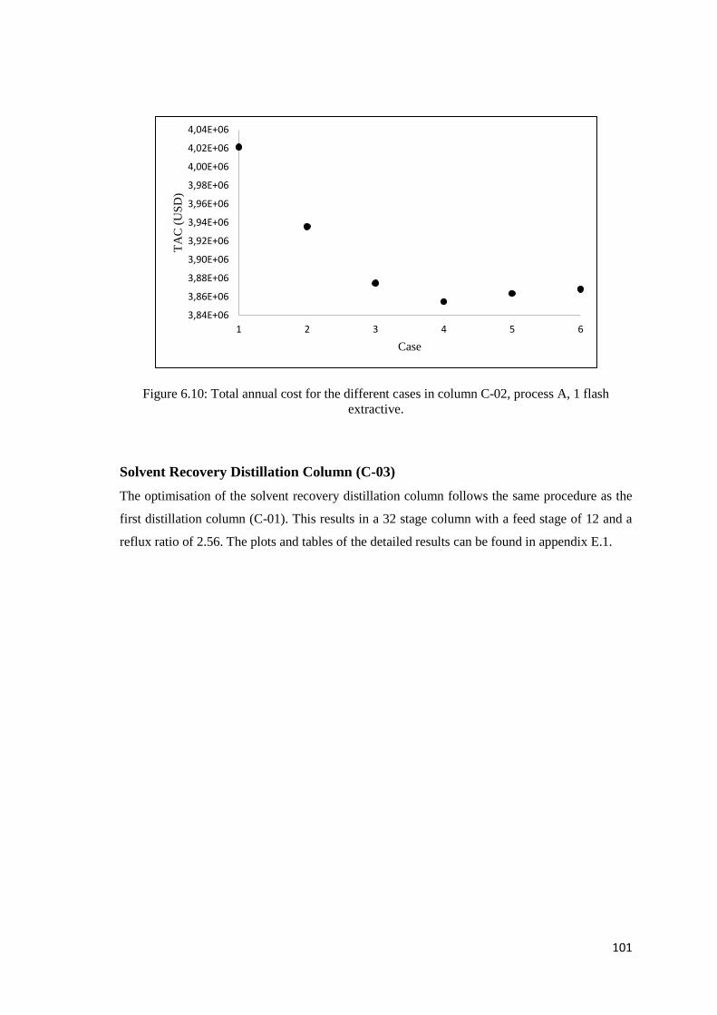
101

Figure 6.10: Total annual cost for the different cases in column C-02, process A, 1 flash

extractive.

Solvent Recovery Distillation Column (C-03)

The optimisation of the solvent recovery distillation column follows the same procedure as the

first distillation column (C-01). This results in a 32 stage column with a feed stage of 12 and a

reflux ratio of 2.56. The plots and tables of the detailed results can be found in appendix E.1.

3,84E+06

3,86E+06

3,88E+06

3,90E+06

3,92E+06

3,94E+06

3,96E+06

3,98E+06

4,00E+06

4,02E+06

4,04E+06

1 2 3 4 5 6

TA

C (

US

D)

Case

102

6.3 Membrane Design

The membrane (pervaporation) was used as an alternative solution to the extractive distillation

process. Hence, in process 1FM, the conventional distillation column (C-01) was followed by the

pervaporation unit replacing columns C-02 and C-03. The membrane network was designed

following the procedure by Wijmans & Baker (1993) as discussed in section 2.4 and Appendix

A. A total flow rate of 20824 kg/hr was fed into the membrane configuration which consisted of

12 modules in parallel by 4 modules in series as shown in Figure 6.11. This configuration was

selected as it proved to be practically possible and economically feasible according to Flemmer,

et al. (1987) and Matteo (2015). Flemmer, et al. (1987) presents possible configurations for spiral

wound modules. In each case an arrangement of 12 modules was considered with 12 modules in

parallel demonstrating a clear superiority over other configurations. Matteo discusses and presents

typical membrane and module specifications to successfully design the process. The aim is to

produce a selective, high flux membrane and to assemble this membrane into compact,

economical membrane modules. The total flow rate was divided by 12 (number of parallel

modules) and fed in equal amounts to each parallel arrangement as shown in the Figure. The

retentate exiting each module becomes the feed to the next module, this is represented by the

black lines in the diagram. The permeate exits the bottom of each module and accumulates to a

single stream, this is represented by the red lines in the diagram.

Feed: 20824 kg/hr

Ethanol: 0.9346

Water: 0.0654

Retentate: 17664.54 kg/hr

Ethanol: 0.9992

Water: 0.0008

Permeate: 3159.46 kg/hr

Ethanol: 0.5753

Water: 0.4247

1735 kg/hr

1735 kg/hr

1735 kg/hr

1735 kg/hr

1735 kg/hr

1735 kg/hr

1735 kg/hr

1735 kg/hr

1735 kg/hr

1735 kg/hr

1735 kg/hr

1735 kg/hr

Figure 6.11: Membrane network configuration

103

Table 6.9 displays the membrane and module specifications. The membrane material, feed

temperature and permeate pressure were specified by Wijmans & Baker (1993). The remaining

specifications were selected for a spiral wound module as specified by Matteo (2015).

Table 6.9: Membrane and module specifications

The first row of the membrane configuration is expanded and displayed in Figure 6.12 to enable

a clear explanation of the process. Firstly, the total flow rate was divided by 12, resulting in a

flow of approximately 1735 kg/hr (which is acceptable for the type of configuration utilised

according to Cao & Henson (2002)) and fed into each parallel arrangement.

Figure 6.12: First row expansion of module configuration

Each module has an area of 20 m2 and 15 envelopes. Therefore, the 4 modules connected in series

in Figure 6.12 has a total area of 80 m2. The retentate exiting each module becomes the feed to

the next module, this is represented by the black lines in the diagram. The permeate exits the

bottom of each module and accumulates to a single stream, this is represented by the red lines in

the diagram. Table 6.10 presents the stream flow rates and compositions for each module

displayed in Figure 6.12.

Membrane Material Poly(vinyl alcohol)

Feed Temperature (oC) 60

Permeate Pressure (kPa) 2.03

Module Spiral wound

Configuration Cross-flow

Inside tube diameter (m) 0.2

Module diameter (m) 0.2032

Module length (m) 1.016

Number of envelopes 15

Membrane Area 20

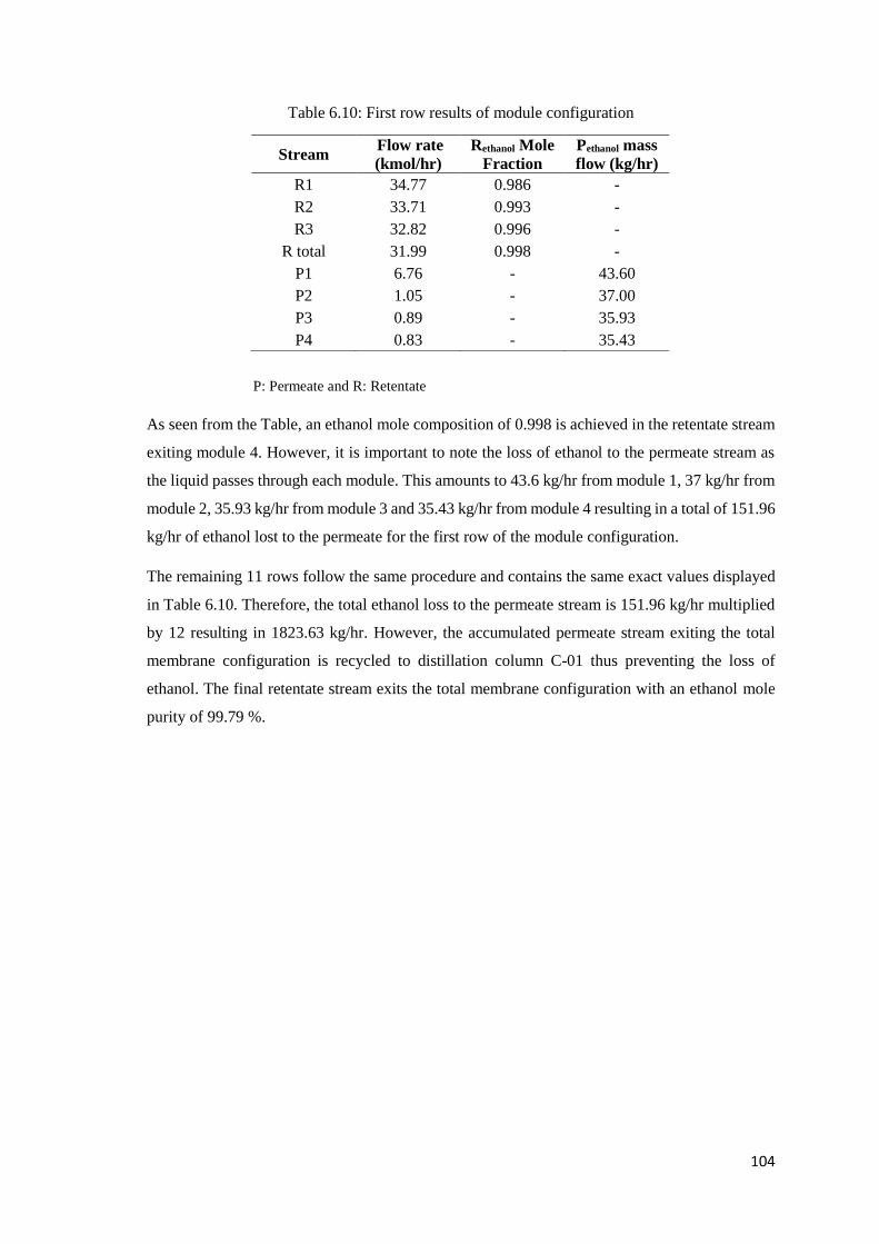
104

Table 6.10: First row results of module configuration

P: Permeate and R: Retentate

As seen from the Table, an ethanol mole composition of 0.998 is achieved in the retentate stream

exiting module 4. However, it is important to note the loss of ethanol to the permeate stream as

the liquid passes through each module. This amounts to 43.6 kg/hr from module 1, 37 kg/hr from

module 2, 35.93 kg/hr from module 3 and 35.43 kg/hr from module 4 resulting in a total of 151.96

kg/hr of ethanol lost to the permeate for the first row of the module configuration.

The remaining 11 rows follow the same procedure and contains the same exact values displayed

in Table 6.10. Therefore, the total ethanol loss to the permeate stream is 151.96 kg/hr multiplied

by 12 resulting in 1823.63 kg/hr. However, the accumulated permeate stream exiting the total

membrane configuration is recycled to distillation column C-01 thus preventing the loss of

ethanol. The final retentate stream exits the total membrane configuration with an ethanol mole

purity of 99.79 %.

Stream Flow rate

(kmol/hr)

Rethanol Mole

Fraction

Pethanol mass

flow (kg/hr)

R1 34.77 0.986 -

R2 33.71 0.993 -

R3 32.82 0.996 -

R total 31.99 0.998 -

P1 6.76 - 43.60

P2 1.05 - 37.00

P3 0.89 - 35.93

P4 0.83 - 35.43

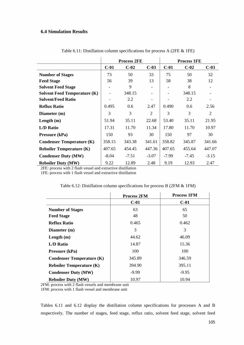
105

6.4 Simulation Results

Table 6.11: Distillation column specifications for process A (2FE & 1FE)

Process 2FE Process 1FE

C-01 C-02 C-03 C-01 C-02 C-03

Number of Stages 73 50 33 75 50 32

Feed Stage 56 39 13 58 38 12

Solvent Feed Stage - 9 - - 8 -

Solvent Feed Temperature (K) - 348.15 - - 348.15 -

Solvent/Feed Ratio - 2.2 - - 2.2 -

Reflux Ratio 0.495 0.6 2.47 0.490 0.6 2.56

Diameter (m) 3 3 2 3 3 2

Length (m) 51.94 35.11 22.68 53.40 35.11 21.95

L/D Ratio 17.31 11.70 11.34 17.80 11.70 10.97

Pressure (kPa) 150 93 30 150 97 30

Condenser Temperature (K) 358.15 343.38 341.61 358.82 345.87 341.66

Reboiler Temperature (K) 407.65 454.45 447.36 407.65 455.64 447.07

Condenser Duty (MW) -8.04 -7.51 -3.07 -7.99 -7.45 -3.15

Reboiler Duty (MW) 9.22 12.89 2.48 9.19 12.93 2.47 2FE: process with 2 flash vessel and extractive distillation

1FE: process with 1 flash vessel and extractive distillation

Table 6.12: Distillation column specifications for process B (2FM & 1FM)

Process 2FM Process 1FM

C-01 C-01

Number of Stages 63 65

Feed Stage 48 50

Reflux Ratio 0.465 0.462

Diameter (m) 3 3

Length (m) 44.62 46.09

L/D Ratio 14.87 15.36

Pressure (kPa) 100 100

Condenser Temperature (K) 345.89 346.59

Reboiler Temperature (K) 394.90 395.11

Condenser Duty (MW) -9.99 -9.95

Reboiler Duty (MW) 10.97 10.94 2FM: process with 2 flash vessels and membrane unit

1FM: process with 1 flash vessel and membrane unit

Tables 6.11 and 6.12 display the distillation column specifications for processes A and B

respectively. The number of stages, feed stage, reflux ratio, solvent feed stage, solvent feed

106

temperature and solvent/feed ratio were determined via the optimisation procedures described in

section 6.2. The values were selected based on either the minimum total annual cost, the minimum

reboiler heat duty or the purity/recovery requirement.

The diameter was calculated using the Aspen Plus® tray sizing function while the length was

calculated by equation 6.3 (typical distance between trays is 0.61 m according to Luyben (2013)).

𝐿 = 1.2 × (𝑇𝑟𝑎𝑦 𝑠𝑝𝑎𝑐𝑖𝑛𝑔) × (𝑁𝑢𝑚𝑏𝑒𝑟 𝑜𝑓 𝑆𝑡𝑎𝑔𝑒𝑠 − 2) 6.3

According to KLM Technology Group (2011), the length/diameter (L/D) ratio of a tower should

be no more than 30 and preferably below 20. As seen from Tables 6.11 and 6.12, the L/D ratios

are well below 20 and hence are acceptable.

The pressures for each column were selected to enable the use of cooling water as the cooling

medium and to prevent the occurance of thermal degradation. It can be seen that the resulting

condenser and reboiler temperatures of 341 – 359 K and 394 – 456 K respectively are high. This

however is due to the high boiling pyridine and ethylene glycol present in the system. The

condenser and reboiler duties were minimised during the optimisation procedure and are also

displayed in the Tables.

Table 6.13 presents the flash vessel specifications for each process. The pressures and

temperatures were selected via the optimisation procedures described in section 6.2. Also

displayed are the column duties.

Table 6.13: Flash vessel specifications

2FE: process with 2 flash vessels extractive distillation

2FM: process with 2 flash vessels and membrane unit



Table 6.14 presents the final flow rates and compositions for the relevant streams in process A. It

can be seen that the mole purities and recoveries of key components ethanol, pyridine and nitrogen

are all greater than 99.9 mol % and hence meet the required specifications as proposed by

NECSA.

Process 1FE utilises one flash vessel and process 2FE utilises two flashes for the nitrogen

separation. As seen from Table 6.14, the nitrogen rich stream for process 1FE still contained 11.36

kg/hr of ethanol. Therefore, this stream was sent to another flash vessel for further purification.

Processes 2FE & 2FM Processes 1FE & 1FM

F-01 F-02 F-01

Pressure (kPa) 200 1930 200

Temperature (K) 248.15 248.15 243.15

Duty (kW) -275.21 -21.38 -291.95

107

As seen from Table 6.14, the additional flash vessel in process 2FE increased the nitrogen purity

by 0.05 % and recovered a further 6.55 kg/hr of ethanol and 0.16 kg/hr of pyridine. Though the

additional flash vessel improved the separation, a cost comparison was required to determine the

its feasibility. This is discussed further in section 6.6.

Table 6.14: Final stream compositions and purities for process A:

Process 2FE Process 1FE

Stream 23 38 37 Recovery 28 38 37 Recovery

Mole Flow (kmol/hr)

Ethanol 0.1044 0.0021 422.33 0.9998 0.2467 0.0021 422.19 0.9998

Water 0.0032 0 0.0519 0.0135 0 0.0413 Pyridine 0.0005 23.17 0 0.9999 0.0024 23.17 0 0.9999

Nitrogen 340.11 0 0.0351 0.9999 340.12 0 0.0268 0.9999

Ethylene Glycol 0 0 0.0059 0 0 0.0174

Mole Fraction Ethanol 0.0003 0.0001 0.9998 0.0008 0.0001 0.9998 Water 0 0 0.0001 0 0 0.0001 Pyridine 0 0.9999 0 0 0.9999 0 Nitrogen 0.9997 0 0.0001 0.9992 0 0.0001 Ethylene Glycol 0 0 0 0 0 0

Mass Flow (kg/hr) Ethanol 4.81 0.0964 19456.28 11.36 0.0965 19450.10 Water 0.0580 0.0040 0.9352 0.2428 0.0040 0.7445 Pyridine 0.0410 1832.71 0.0008 0.1922 1832.55 0 Nitrogen 9527.60 0 0.9828 9527.84 0 0.7505 Ethylene Glycol 0 0 0.3692 0 0 1.08

Mass Fraction Ethanol 0.0005 0.0001 0.9999 0.0012 0.0001 0.9999 Water 0 0 0 0 0 0

Pyridine 0 0.9999 0 0 0.9999 0 Nitrogen 0.9995 0 0.0001 0.9988 0 0 Ethylene Glycol 0 0 0 0 0 0.0001

Total Flow (kg/hr) 9532.51 1832.81 19458.56 9539.63 1832.66 19452.67

Temperature (K) 248.15 407.65 343.38 243.15 407.65 345.87

Pressure (kPa) 1930 179.49 93 200 179.48 97 2FE: process with 2 flash vessels and extractive distillation


Table 6.15 presents the final flow rates and compositions for the relevant streams in process B.

Process 1FM utilises one flash vessel and process 2FM utilises two flashes for the nitrogen

separation. As seen from Table 6.15, the use of the additional flash vessel increased the nitrogen

108

purity by 0.05 % and recovered a further 6.55 kg/hr of ethanol and 0.15 kg/hr of pyridine similarly

to process A.

It is also observed that an ethanol mole recovery of 90.64 % was obtained in the retentate stream

resulting in an ethanol loss of 1823.63 kg/hr (9.36 %) to the permeate stream. However, this

stream was recycled to the distillation column preventing any loss of chemical. The addition of

this stream to the distillation column shifts the feed composition such that the separation of

pyridine becomes more difficult. As seen in Table 6.15, the maximum allowable recovery and

purity of pyridine is 99.5 mol % (as opposed to the 99.99 mol % achieved with extractive

distillation).

An ethanol mole purity of 99.79 % was obtained in the retentate stream. The total membrane area

discussed in section 6.3 could have been increased to improve the ethanol purity however, the

separation became extremely slow as the amount of water decreased. The retentate stream

contains a water content of 0.21 mol %; had this stream been dehydrated to a water content of

0.01 mol % (like the purity obtained in extractive distillation), the total membrane area would

have increased to a value of 2000 m2 resulting in a cost of 8 million euros (Wolf, 2017). The area

required for the membrane then becomes practically and economically unfeasible. Furthermore,

increasing the membrane area, increases the flow rate of the recycle stream (permeate) thereby

decreasing the allowable recovery and purity of the core component, pyridine. A cost evaluation

was performed and is discussed further in section 6.6.

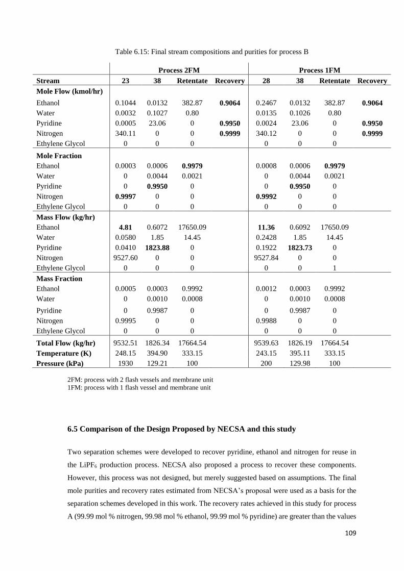
109

Table 6.15: Final stream compositions and purities for process B

Process 2FM Process 1FM

Stream 23 38 Retentate Recovery 28 38 Retentate Recovery

Mole Flow (kmol/hr)

Ethanol 0.1044 0.0132 382.87 0.9064 0.2467 0.0132 382.87 0.9064

Water 0.0032 0.1027 0.80 0.0135 0.1026 0.80 Pyridine 0.0005 23.06 0 0.9950 0.0024 23.06 0 0.9950

Nitrogen 340.11 0 0 0.9999 340.12 0 0 0.9999

Ethylene Glycol 0 0 0 0 0 0

Mole Fraction Ethanol 0.0003 0.0006 0.9979 0.0008 0.0006 0.9979 Water 0 0.0044 0.0021 0 0.0044 0.0021 Pyridine 0 0.9950 0 0 0.9950 0 Nitrogen 0.9997 0 0 0.9992 0 0 Ethylene Glycol 0 0 0 0 0 0

Mass Flow (kg/hr) Ethanol 4.81 0.6072 17650.09 11.36 0.6092 17650.09 Water 0.0580 1.85 14.45 0.2428 1.85 14.45 Pyridine 0.0410 1823.88 0 0.1922 1823.73 0 Nitrogen 9527.60 0 0 9527.84 0 0 Ethylene Glycol 0 0 0 0 0 1

Mass Fraction Ethanol 0.0005 0.0003 0.9992 0.0012 0.0003 0.9992 Water 0 0.0010 0.0008 0 0.0010 0.0008

Pyridine 0 0.9987 0 0 0.9987 0 Nitrogen 0.9995 0 0 0.9988 0 0 Ethylene Glycol 0 0 0 0 0 0

Total Flow (kg/hr) 9532.51 1826.34 17664.54 9539.63 1826.19 17664.54

Temperature (K) 248.15 394.90 333.15 243.15 395.11 333.15

Pressure (kPa) 1930 129.21 100 200 129.98 100



6.5 Comparison of the Design Proposed by NECSA and this study

Two separation schemes were developed to recover pyridine, ethanol and nitrogen for reuse in

the LiPF6 production process. NECSA also proposed a process to recover these components.

However, this process was not designed, but merely suggested based on assumptions. The final

mole purities and recovery rates estimated from NECSA’s proposal were used as a basis for the

separation schemes developed in this work. The recovery rates achieved in this study for process

A (99.99 mol % nitrogen, 99.98 mol % ethanol, 99.99 mol % pyridine) are greater than the values

110

reported by NECSA (95.00 mol % nitrogen, 99.80 mol % ethanol, 99.99 mol % pyridine) for all

three components whilst the recovery rates achieved in process B (99.99 mol % nitrogen, 100 mol

% ethanol, 99.50 mol % pyridine) are greater than NECSA’s proposal for nitrogen and ethanol

but 0.49 mol % lower for pyridine. The mole purities obtained in process A for ethanol (99.98 %)

and pyridine (99.99 %) were also greater than the mole purities stated by NECSA (99.98 %

ethanol, 97.76 % pyridine) whilst the mole purities obtained in process B was greater for pyridine

(99.5 %) and slightly lower for ethanol (99.79%). The nitrogen mole purity in both processes A

& B (99.97 %) was slightly lower than NECSA’s proposal (99.99 %). However, it is important to

note that in NECSA’s recycle process proposal, some of the assumptions made were inaccurate.

For example, it is assumed that 100 % of the nitrogen entering a gas permeation unit is removed

in the permeate. This is unlikely. Furthermore, NECSA’s separation scheme could not be

designed and verified since an extensive search showed that there is currently no permeation flux

data for the systems of interest in the open literature. Without this data, the membranes could not

be designed. Therefore, in terms of the overall mole purities and recovery rates, the processes

developed in this work achieves a better separation.

6.6 Cost Evaluation

Table 6.16 is a summary of the capital and operating costs for processes developed in this study.

The capital investment cost of the membrane and modules were calculated manually on Microsoft

Excel. This involved multiplying the membrane/module area by the typical costs obtained in

literature. The total membrane/module area required was calculated using the methodology by

Wijmans & Baker (1993) shown in appendix A. The capital investment cost of all other units

were evaluated using the Aspen Plus® computer software. The operating costs were determined

by means of the utility correlations and prices obtained in literature. A detailed explanation is

provided in Appendix B. In Table 6.16, the total capital investment costs, operating costs and total

annual costs are highlighted in bold.

111

Table 6.16: Capital and operating cost summary

Equipment Cost (R 103/hr) Process A (2FE) Process A (1FE) Process B (2FM) Process B (1FM)

F-01-flash vessel 394.95 394.95 394.95 394.95

F-02-flash vessel 541.85 541.85

P-01-pump 60.21 60.21 60.21 60.21

P-02-pump 61.41 61.41 62.61 62.61

C-01-condenser 462.38 459.97 622.53 618.92

C-01-reflux drum 180.62 149.31 181.82 181.82

C-01-reboiler 1201.71 1199.31 1080.10 1080.10

C-01-reflux pump 60.21 60.21 61.41 61.41

C-01-tower 7687.11 7887.00 6666.02 6939.35

C-02-condenser 511.75 496.10

C-02-reflux drum 181.82 181.82

C-02-reboiler 1326.94 1334.17

C-02-reflux pump 60.21 60.21

C-02-tower 5439.02 5439.02

C-03-condenser 233.60 236.01

C-03-reflux drum 181.82 181.82

C-03-reboiler 385.32 385.32

C-03-reflux pump 51.78 51.78

C-03-tower 2591.27 2449.18

HX-01-cooler 396.16 396.16

Membrane

Module

Total Capital (R 103) 22010.14 21483.94 13120.43 12848.30

112

Operating Costs (R 103/year) Process A (2FE) Process A (1FE) Process B (2FM) Process B (1FM)

P-01 5.94 5.94 5.94 5.94

P-01 10.50 10.50 5.82 5.82

F-01 2079.95 2206.41 2079.95 2206.41

F-02 161.59 161.59 C-01 condenser 980.72 974.47 1218.44 1213.41

C-01 reboiler 10164.18 10122.91 16710.19 12058.44

C-02 condenser 915.41 908.56

C-02 reboiler 19712.51 19778.24

C-03 condenser 374.54 383.92

C-03 reboiler 3793.76 3778.93

HX-01 620.88 618.92

Solvent make up 68.00 113.94

Refrigeration

Feed Cooler

Vacuum Pump

Inter-stage Heaters

Total 38887.97 38902.75 30515.36 25823.46

Solvent 550.90 500.90

Replacement 1842.99 1842.99

Total Operating Costs (R 103/year) 39438.87 39453.65 32358.35 27666.45

TAC (R 103) 46041.91 45898.83 36294.48 31520.94

113

The total annual cost of the processes including extractive distillation are much larger than the

processes with the membranes. However, the total membrane area required (960 m2) is large and

the membrane process allows a recovery and purity of only 99.5 mol % pyridine as opposed to

the 99.99 mol % achieved with extractive distillation. Furthermore, the capital investment cost of

the membrane was calculated based on estimates (such as membrane and module cost, structural

arrangement and flow rate allowance) from one research paper and the total area calculated was

restricted to 960 m2 due to the reduction in pyridine recovery and purity. The retentate stream

contains a water content of 0.21 mol %; had this stream been dehydrated to a water content of

0.01 mol % (similar to the purity obtained in extractive distillation), the pyridine loss, total

membrane area and capital costs would have increased significantly.

The processes with two flash vessels have higher capital and operating costs than the processes

with one flash vessel. The higher capital cost is due to the costs associated with purchasing and

installing an additional unit. The higher operating cost is due to the additional liquid flow rate

recovered of 7.12 kg/hr (comprising pyridine, ethanol and water) which is sent to the distillation

columns resulting in higher flow rates and hence higher operating costs (for example, more steam

or cooling water will be required to heat/cool process streams). The cost difference between

processes 1FE and 2FE is minimal (R0.14 million). The cost difference between processes 1FM

and 2FM is significant (R5 million).

Table 6.17 includes the final mole purity, mole flow and mass flow for each component after

separation. It can be seen that processes 1FM and 2FM show little to no change and the only

significant change between processes 1FE and 2FE is the additional 6.18 kg/hr of ethanol

recovered with two flash vessels.

114

Table 6.17: Purity and flow rate of relevant streams

Mole Purity Process 2FE Process 1FE Process 2FM Process 1FM

Nitrogen 0.9997 0.9992 0.9997 0.9992

Pyridine 0.9999 0.9999 0.9950 0.9950

Ethanol 0.9998 0.9998 0.9979 0.9979

Ethylene Glycol Recycle 0.9999 0.9999

Mole Flow (kmol/hr) Nitrogen 340.11 340.12 340.11 340.12

Pyridine 23.17 23.17 23.06 23.06

Ethanol 422.33 422.19 382.87 382.87

Ethylene Glycol Recycle 1095.98 1095.97

Mass (kg/hr) Nitrogen 9527.60 9527.84 9527.60 9527.84

Pyridine 1832.71 1832.56 1823.88 1823.73

Ethanol 19456.28 19450.10 17650.09 17650.09

Ethylene Glycol Recycle 68025.96 68025.25 2FE: process with 2 flash vessels and extractive distillation




Therefore, the use of the additional flash vessel in process B is infeasible due to the significant

increase in cost and little to no improvement in component flows. The use of the additional flash

vessel in process A however recovers more ethanol and contains a purer nitrogen stream whilst

increasing the total annual cost by only R0.14 million thereby proving its feasibility.

Figures 6.13 and 6.14 display an operating cost summary of the two processes developed, showing

the major utility costs. It can be seen that the highest contributors are the steam requirement for

the reboilers and the refrigerant required for permeate condensing.

115

Figure 6.13: Operating cost summary for process A (process with extractive distillation)

Figure 6.14: Operating cost summary for process B (process with membranes)

0,0E+00

5,0E+06

1,0E+07

1,5E+07

2,0E+07

2,5E+07

Ran

ds

Process A

2 Flash 1 Flash

0,0E+002,0E+064,0E+066,0E+068,0E+061,0E+071,2E+071,4E+071,6E+071,8E+07

Ran

ds

Process B

2 Flash 1 Flash

116

CHAPTER 7: CONCLUSION

A novel process for the production of lithium hexafluorophosphate (LiPF6) was developed by

NECSA. The purpose of this study was the design and economic evaluation of a process to treat

the waste streams (comprising pyridine, ethanol, water and nitrogen) leaving the LiPF6 production

process. The objective was to separate and recover these components such that they could be

recycled and reused in the LiPF6 production.

The design and development of separation processes rely on accurate vapour liquid equilibrium

(VLE) data. The ethanol/pyridine (40 kPa, 100 kPa, 313.15 K) and water/pyridine (40 kPa, 333.15

K) phase data were measured since the VLE data found in literature for these systems were

inconsistent. A modified recirculating VLE still was used to measure the phase equilibrium data

with sample analysis performed using a Shimadzu GC-2014.

The measured data was regressed using various thermodynamic models in Aspen Plus®. The

model that best suited the components of interest was the Peng-Robinson equation of state


NRTL activity coefficient model (PR-MC-WS-NRTL). The binary parameters obtained with the

use of this model was then incorporated into the Aspen Plus® computer software where it was

used to simulate proposed process schemes.

The ethanol/water system was not measured since there is a wide range of consistent VLE data

available for this system. Aspen Plus® stores physical property parameters for numerous

components in several databanks which are developed from the thermodynamic models available

and data from the Dortmund Databank. Hence the built-in parameters from Aspen Plus® for the

ethanol/water system was used for the design.

A mixture of four components (nitrogen, ethanol, water and pyridine) required separation and

recovery. Nitrogen could easily be removed with the use of a flash vessel. The behaviour of the

remaining components (ethanol, water and pyridine) was studied and residue curve maps drawn

to determine the type of separation expected. It was observed from these diagrams that pyridine

could be separated via conventional distillation. The separation of ethanol and water however,

required the use of an enhanced separation technique due to the azeotrope formed. Extractive

distillation and pervaporation were selected to separate ethanol from water since these are

common and simple processes, less energy intensive than the alternatives and can handle the feed

capacity.

Two separation schemes were investigated. Process A treats the waste stream firstly via a flash

vessel to remove the nitrogen, then a conventional distillation column to separate the pyridine

from the mixture followed by an extractive distillation column to separate the ethanol from water.

117

The solvent chosen for extractive distillation was ethylene glycol since it is less energy intensive

than its alternative liquid solvents and ionic liquids and contains no unwanted entrainment (solid

salt) into the product or equipment. Process B follows the same scheme as process A for the

nitrogen and pyridine separation; however it uses a pervaporation membrane modular setup,

incorporating a polyvinylalcohol (PVA) membrane in a spiral wound configuration, to break the

ethanol/water azeotrope as opposed to the use of the extractive distillation column use in process

A. PVA was selected as the membrane material since an extensive search showed that the only

permeation flux data available in the open literature was one which used a PVA membrane. The

spiral wound module was selected since it is simpler and less expensive than its alternatives.

Modifications were made to each process where an additional flash vessel was used to further

purify the nitrogen stream. Pyridine and water separated from nitrogen easily; however,

separating the ethanol was more challenging. Therefore, this additional flash vessel was utilised

to separate the remaining ethanol from nitrogen.

The membranes were designed on Microsoft Excel, while all other units were deigned on Aspen

Plus®. The flash vessels and distillation columns were optimised using sensitivity analysis plots.

These are graphs that vary variables such as temperature, pressure, number of stages, feed stage

location, reflux ratio, etc. against mole purities, column duties and total costs. The membranes

were designed following a procedure from a research paper.

The final mole purity and recovery rate of nitrogen was >99.9 mol % for all processes. The ethanol

and pyridine mole purities and recovery rates for the extractive distillation processes were also

>99.9 mol %. Regarding the membrane processes, the pyridine purity and recovery was 99.5 mol

% while the ethanol purity was 99.79 mol % with a recovery of 100 mol % (since the permeate

was recycled).

The economic analysis showed that while process A met the specified purity and recovery of 99.9

mol %, it had a high total annual cost (approximately R46 million) due to the large amount of

solvent required for extractive distillation. Process B using the modular membrane setup, had a

significantly lower total annual cost (approximately R32 million). However, this is due to the area

restriction imposed on the membrane (960 m2) due to the pyridine loss and slow separation

process as the water composition decreased. The ethanol-rich stream (retentate) leaving the

membrane unit contained a water content of 0.21 mol %; had this stream been dehydrated to a

water content of 0.01 mol % (similar to the purity obtained with extractive distillation), the total

membrane area would have increased to a value of 2000 m2 resulting in a cost of 8 million euros.

The area required for the membrane then becomes practically and economically unfeasible.

Furthermore, increasing the membrane area, increases the flow rate of the recycle stream

(permeate) thereby decreasing the allowable recovery and purity of the core component, pyridine.

118

The use of the additional flash vessel in process B was not economically feasible due to the

significant increase in cost (R4 million) and little to no improvement in final component purities.

However, the additional flash vessel in process A recovered a further 6.18 kg/hr of ethanol

producing a purer nitrogen stream whilst slightly increasing the total annual cost by R0.14 million.

To conclude, process B does not meet the purity and recovery specifications for pyridine and

ethanol. If it is attempted to achieve the ethanol purity specification, the membrane process

becomes impractical due to the large membrane area required and the recovery and purity of the

core component pyridine decreases. Furthermore, the additional flash vessel used in this process

significantly increases the total annual cost and does not improve the product purities. Process A

meets the required purity and recovery specifications for all components and is practically

feasible. The additional flash vessel used in this process recovers a further 6.18 kg/hr of ethanol

whilst slightly increasing the total annual cost and hence is the optimal solution.

119

CHAPTER 8: RECOMMENDATIONS

The extractive distillation processes have a large total annual cost. This is due to the high solvent

to feed ratio, high liquid phase load and great amount of solvent recycling resulting in a high

consumption of energy. A combination of ethylene glycol and calcium chloride salt should be

investigated. The addition of the salt increases the relative volatility of the ethanol-water system

thereby reducing the number of theoretical stages, the amount of solvent required and hence the

energy consumption. Furthermore, mixing the solid salt with ethylene glycol allows utilising the

advantages of both components and reduces the shortcomings such as corrosion caused by the

salt and high energy consumption by the liquid solvent.

Experiments on the ethanol/water/pyridine, ethanol/water and pyridine/water systems should be

performed to determine the permeation fluxes for a membrane design. This will allow the

selection of a more suitable membrane material and numerous possibilities for the design

procedure.

Different membrane modules should be investigated. Other modules could possibly produce a

simpler configuration with lower area and cost requirements.

Heat integration is a technique utilised to minimise energy consumption and maximise heat

recovery in a chemical process. This is done by recovering heat that was previously cooled off

and reusing it in another unit operation. This task minimises the operating costs as it reduces the

utility requirements such as steam and cooling water. This however was not performed in this

research project as the process designed is not the entire plant but just a sector. Heat integration

should be performed on the entire process (this study along with LiPF6 production process), this

would give a better representation of the total costs.

120

REFERENCES

Abbott, M., 1979. Cubic Equations of State: An Interpretive Review. Troy, New York:

Department of Chemical and Environmental Engineering, Rensselaer Polytechnic Institute.

Abe, J., Nakanishi, K. & Touhara, H., 1978. Thermodynamic properties of aqueous solutions of

hydrophilic compounds 1. pyridine and methylpyridines. Journal of Chemical Thermodynamics,

Issue 10, pp. 483 - 494.

Abrams, D. & Prausnitz, J., 1975. Statistical thermodynamics of liquid mixtures: A new

expression for the excess Gibbs energy of partly or completely miscible systems. AIChE

Journal, 21(1), pp. 116-128.

Abu Al-Rub, F. & Datta, R., 2001. Chemical Engineering Journal, pp. 81 - 83.

Allen, M., 2007. The Physics Factbook. [Online]

Available at: http://hypertextbook.com/facts/2007/AllenMa.shtml

[Accessed 20 July 2015].

Andon, R., Cox, J. & Herington, E., 1957. Phase relationships in the pyridine series. Part 6. The

thermodynamic properties of mixtures of pyridine, and of the three of its homologues, with

water. Transactions of the Faraday Society, I(53), pp. 410-426.

AspenTech, 2015. Aspen Plus Help. Bedford, Massachusetts: Aspen Technology Inc.

Bastidas, P., Gil, I. & Rodrígueza, G., 2010. Comparison of the main ethanol dehydration

technologies through process simulation, Colombia: Elsevier.

Beebe, A., Coulter, K., Lindsay, R. & Baker, E., 1942. Equilibria in Ethanol-Water System at

Pressures less than atmospheric. Journal of Industrial and Engineering Chemistry, Issue 34, pp.

1501 - 1504.

Bhownath, R., 2008. The Use of n-Dodecane as a Solvent in the Extraction of Light Alcohols

from Water, Master of Science in Engineering (Chemical Engineering) Thesis: University of

KwaZulu-Natal, South Africa.

Cao, B. & Henson, M., 2002. Modeling of spiral wound pervaporation module with application

to the separation of styrene/ethylbenzene mixtures. Journal of Membrane Science, I(197), pp.

117-146.

Chaplin, M., 2017. Water Structure and Science. [Online]

Available at: http://www1.Isbu.ac.uk/water/water_properties.html

[Accessed 26 May 2017].

Chemical Engineering Online, 2008. Chemical Engineering Cost Indicies. [Online]

Available at:

http://www.engr.uconn.edu/~ewanders/Design/Chemical%20Engineering%20Cost%20Indices

%20Jan%202008.pdf

[Accessed 15 September 2016].

Chemical Engineering Online, 2016. Economic Indicators. [Online]

Available at: tekim.undip.ac.id/v1/wp-content/uploads/CEPCI_2008_2015.pdf

[Accessed 15 September 2016].

121

ChemicalBook, 2016. Cyclohexane. [Online]

Available at: http://www.chemicalbook.com/ChemicalProductProperty_EN_CB4193601.htm

[Accessed 30 January 2016].

Cheng, R., Cho, C. H., Kirby, S. & Lim, B., 2010. Economic recovery of pyridine and 3-

methylpyridine, Pennsylvania: Scholarly Commons.

Chirico, R. et al., 1996. Thermodynamic properties of pyridine I. Vapor pressures, high-

temperature heat capacities, densities, critical properties, derived thermodynamic functions,

vibrational assignment, and derivation of recommended values. J.Chem, 28(8), pp. 797-818.

Crew, C. & Schafer, T., 1993. Recovery of Pyridine Saves $1.5 Million Per. s.l.:Pharmaceutical

Engineering.

Daniel, C., 2008. Materials and Processing for Lithium-ion Batteries. The Member Journal of

the Minerals, Metals & Minerals Society, 60(9), pp. 43-48.

D'Avila, S. & Silva, R., 1970. Isothermal vapor-liquid equilibruim data by total pressure

method. Journal of Chemical Engineering Data, 3(15), pp. 421-424.

Dharmendira Kumar, M. & Rajendran, M., 1998. Effect of dissolved salts on the vapor-liquid

equilibrium relationships of three miscible binary systems at the pressure of 101.3 kPa. Journal

of Chemical Engineering, Issue 31.

Dortmund Data Bank, 2015. Vapour Pressure of Ethanol. [Online]

Available at: www.ddbst.com/ddb.html

[Accessed 28 August 2015].

Ewert, M., 1936. Theory of concentrated solutions. XII Aq. soln. of organic compounds.

Bulletin des Societes Chimiques Belges, Issue 45, p. 493.

Findlay, T. & Copp, J., 1969. Thermodynamics of binary systems containing amines. Part 5 -

Alcohols and Pyridine. Transactions of the Faraday Society, 65(558), pp. 1463-1469.

Flemmer, R., Buckley, C. & Groves, G., 1987. The Arrangement of Spiral-Wound Ultrafiltraion

Modules. Desalination, I(61), pp. 159-168.

Fowler, R., 1949. A modified vapour liquid equilibrium still. J.S.C.I, Volume 68, pp. 131-132.

Fowler, R., 1952. Azeotropism in binary solutions at reduced pressures: III pyrdine + water

solution. Jounal of Applied Chemistry, Issue 2, p. 246.

Gierycz, P., 1996. Vapor pressures and activity coefficients at infinite dilution of (water +

pyridine, or 2-methylpyridine, or 3-ethylpyridine, or 2,4,6- trimethylpyridine) at T = 353.15 K.

Journal of Chemical Thermodynamics, Issue 28, pp. 343 - 347.

Gil, I., Garcia, L. & Rodriguez, G., 2014. Simulation of Ethanol Extractive Distillation with

Mixed Glycols as Separating Agent. Brazilian Journal of Chemical Engineering, 31(1), pp.

259-270.

Gil, I. et al., 2008. Separation of Ethanol and Water by Extractive Distillation with Salt and

Solvent as Entrainer: Process Simulation. Brazilian Journal of Chemical Engineering, 25(1), pp.

207-215.

Gutierrez H, J., 2013. Extractive Distillation with Ionic Liquids as Solvents: A Conceptual

Process Design, Netherlands: Eindhoven University of Technology.

122

Harris, D., 2011. refractometer.pl. [Online]

Available at: http://www.refractometer.pl/refraction-datasheet-ethanol


Haynes, W., 2011. CRC Handbook of Chemistry and Physics. 91st ed. Boca Raton: CRC Press

Inc.

Heertjies, P., 1060. Determination of Vapour-Liquid Equilibrium of Binary Mixtures. Chemical

and Process Engineering, Volume 41, pp. 385-386.

Holderbaum, B. & Gmehling, J., 1991. PSRK: A Group Contribution Equation of State based

on UNIFAC. Fluid Phase Equilibria, Volume 70, pp. 251-265.

Ibl, N., Daendliker, G. & Truempler, G., 1954. Uber das Verdampfungsgleichgewicht des

systems wasser - pyridin. Helvetica Chemica Acta, I(37), pp. 1661-1672.

Ibl, N., Dandliker, G. & Trumpler, G., 1956. The Vapour-Liquid Equilibrium of the System

Water-Pyridine. Chemical Engineering Science, Issue 5, p. 193.

Janaszewski, P., Oracz, P., Goral, M. & Warycha, S., 1982. Vapour-Liquid Equilibria. I. An

Apparatus for Isothermal Total Vapour Pressure Measurements: Binary Mixtures of Ethanol and

t-Butanol with n-Hexane, n-Heptane and n-Octane at 313.15 K. Fluid Phase Equilibria, Issue 9,

pp. 295-310.

Jobson, M., 2014. Energy Considerations in Distillation. In: Distillation: Fundamentals and

Principles. Manchester: Elsevier, pp. 225-270.

Joseph, M., Raal, J. & Ramjugernath, D., 2001. Phase Equilibrium Properties of Binary Systems

with Diacetyl from a Computer Controlled Vapour-Liquid Equilibrium Still. Fluid Phase

Equilibria, Volume 182, pp. 157-176.

Kaewkannetra, P. et al., 2012. Experimental study and cost evaluationfor ethanol separation

from fermentation broth using pervaporation. Desalination and Water Treatment, I(41), pp. 88-

94.

Khattab, I. S., Bandarkar, F., Fahkree, M. A. A. & Jouyban, A., 2012. Density, viscosity, and

surface tension of water+ethanol mixtures from 293 to 323K. Korean Journal of Chemical

Engineering, 29(6), pp. 812-817.

KLM Technology Group, 2011. Distillation Column Selection and Sizing (Engineering Design

Guidelines). [Online]

Available at:

http://kolmetz.com/pdf/EDG/ENGINEERING%20DESIGN%20GUIDELINES%20-

%20distillation%20column%20-%20Rev%2003%20web.pdf


Kneisl, P., Zondlo, J. & Wallace, B., 1989. The Effect of Fluid Properties on Ebulliometer

Operation. Fluid Phase Equilibria, Volume 46, pp. 85-94.

Kontogeorgis, G. & Folas, G., 2009. Thermodynamic Models for Industrial Applications: From

Classical and Advanced Mixing Rules to Association Theories. s.l.:Wiley.

Kujawski, W., 2000. Application of Pervaporation and Vapor Permeation in Environmental

Protection. Polish Journal of Environmental Studies, 9(1), pp. 13-26.

Kumar, M., Dixit, S. K., Singh, S. K. & Agarwal, A., 2010. Eco-friendly process for recovery of

pyridine and/or its derivatives. United States, Patent No. US 20100041894 A1.

123

Kumar, M., Dixit, S., Singh, S. & Agarwal, A., 2011. Eco-friendly Process for Recovery of

Pyridine. United States, Patent No. US8057643 B2.

Kyte, C. T., Jeffery, G. H. & Vogel, A. I., 1960. Physical Properties and Chemical Constitution.

Part XXVIII.* Pyridine Derivatives. Journal of the Chemical Society, pp. 4454-4472.

Lekgoathi, M., Crouse, P. & Kock, L., 2015. High purity LiPF6: its physical properties and the

synthesis of PF5 gas as a precursor for LiPF6 production, Pretoria: University of Pretoria.

Lie, Z., Li, C. & Chen, B., 2003. Extractive Distillation: A Review. Separation and Purification

Reviews, 32(2), pp. 121-213.

Lladosa, E., Monton, J. & Burguet, M., 2011. Chemical Engineering and Processing. Separation

of di-n-propyl ether and n-propyl alcohol by extractive distillation and pressure-swing

distillation: Computer simulation and economic optimisation, I(50), pp. 1266-1274.

Luyben, W., 2013. Distillation Design and Control Using Aspen Simulation. 2nd ed. Canada:

John Wiley & Sons, Inc..

Matteo, G., 2015. Membrane modules and configurations. Zurich: Separation Process

Laboratory.

MEGlobal, 2017. Physical Properties of Ethylene Glycol. [Online]

Available at: http://www.meglobal.biz/monoethylene-glycol/physical-properties


Munoz, R., Monton, J., Burguet, M. & de la Torre, J., 2006. Separation and Purification

Technology. Separation of isobutyl alcohol and isobutyl acetate by extractive distillation and

pressure-swing distillation: Simulation and Optimisation, I(50), pp. 175-183.

Naidoo, M., 2014. Thermodynamic properties of mixtures containing ethanol, water and

pyridine, University of KwaZulu-Natal, South Afrca: Chemical Engineering Vacation Work

Project .

Narasigadu, C., 2006. Phase Equilibrium Investigation of the Water and Acetonitrile Solvent

with Heavy Hydrocarbons, Master of Science in Engineering (Chemical Engineering) Thesis:

University of KwaZulu-Natal, South Africa.

Ndlovu, M., 2005. Development of a Dynamic Still for Measuring Low Pressure Vapour-

Liquid-LiquidEquilibria (Systems of Partial Liquid Miscibility), Master of Science in

Engineering (Chemical Engineering) Thesis: University of KwaZulu-Natal, South Africa.

NECSA, 2017. Personal Communication. Pretoria: NECSA.

Nelson, W., 2012. Separation of Trichlorosilane: Measurement, Modelling and Simulation,

Doctor of Philisophy in Engineering (Chemical Engineering) Thesis: University of KwaZulu-

Natal, South Africa.

Ocic, O., 2012. Energy Efficiency in Oil Processing Industry. Europe: European Commision.

Orbey, H. & Sandler, S., 1998. Modeling vapor-liquid equilibria: cubic equations of state and

their mixing rules, s.l.: Cambridge University Press.

Perry, R. & Green, D., 1999. Perry's Chemical Engineers' Handbook. 7th ed. New York:

McGraw-Hill.

Pickering, S., 1893. A study of the properties of some strong solutions. Journal of Chemical

Society, Issue 63, pp. 998-1027.

124

Pokki, J., 2004. Development of Vapour Liquid Equilibrium, Doctor of Science in Technology

Thesis: Helsinki University of Technology, Finland, Espoo.

Prausnitz, J. M. & Targovnik, J., 1958. Salt effects in aqueous vapor-liquid equilibria. Chemical

Engineering Data Series, Issue 3, p. 124.

PubChem, 2004. Pyridine. [Online]

Available at: http://pubchem.ncbi.nlm.nih.gov/compound/pyridine#section=Top


PubChem, 2015. Cyclohexane. [Online]

Available at: http://pubchem.ncbi.nlm.nih.gov/compound/cyclohexane


PubChem, 2015. Pyridine. [Online]

Available at: http://pubchem.ncbi.nml.nih.gov/compound/pyridine#section=Information-

Sources


Raal, J. & Muhlbaüer, A., 1998. Phase Equilibria: Measurement and Computation.

Washington, D.C: Taylor and Francis.

Rarey, J., 2017. Personal Communication. University of Oldenburg: Germany.

Renewable Energy, 2017. Renewable Energy South Africa. [Online]

Available at: https://renewableenergy.co.za

[Accessed 03 01 2017].

Renon, H. & Prausnitz, J., 1968. Local compositions in thermodynamic excess functions for

liquid mixtures. AIChE Journal, Issue 14, pp. 135-144.

Sadus, R., 2012. High Pressure Phase Behaviour of Multicomponent Fluid Mixtures , s.l.:

Elsevier Science.

Safobeen, S., 2011. Plant for Separation of Styrene, Ethyl Benzene, Ammonia and Hydrogen

Sulfide, New York: s.n.

Sandler, S., 1994. Models for thermodynamic and phase equilibria calculations, s.l.: Dekker.

Satkiewicz, F., 1964. The System Ethanol-Cyclohexane from 50 to 65°. J.Am.Chem.Soc.,

Volume 86, pp. 130-133.

Scatchard, G., Wood, S. & Mochel, J., 1939. III. Benzene - Cyclohexane Mixtures. Journal of

Physical Chemistry, Volume 43, pp. 119-130.

Schiffmann, P., 2014. Three step modelling approach for the simulation of industrial scale

pervaporation modules, Freiberg: Technische Universität Bergakademie Freiberg.

Seader, J., Henley, E. & Roper, D., 2011. Separation Process Principles: Chemical and

Biochemical Operations. 3rd ed. United States of America: John Wiley & Sons.

Taylor, B. & Kuyatt, C., 1994. Guidelines for evaluating and expressing the uncertainty of NIST

measurement results: NIST Technical Note 1297, Gaithersburg: National Institute of Standards

and Technology.

The Money Converter, 2016. The Money Converter. [Online]

Available at: https://themoneyconverter.com/EUR/ZAR.aspx

[Accessed 10 December 2016].

125

TradeKey, 2016. AJL Chemical Trading. [Online]

Available at: http://www.tradekey.com/product_view/Mono-Ethylene-Glycol-meg--

7696007.html


Twu, C., Sim, W. & Tassone, V., 2002. Getting a handle on advanced cubic equations of state..

Chemical Engineering Progress, Issue 98, pp. 58-65.

USGS, 2016. Surface Tension and Water. [Online]

Available at: http://water.usgs.gov


Van Hoof, V. et al., 2004. Separation and Purification Technology. Economic comparison

between azeotropic distillation and different hybrid systems combining distillation with

pervaporation for the dehydration of isopropanol, I(37), pp. 33-49.

Vesovic, V., 2011. Thermopedia. [Online]

Available at: http://www.thermopedia.com/content/739/


Vriens, G. N. & Medcalf, E. C., 1953. Correlation of ternary liquid-liquid equilibria an

explanation of solutropy. Journal of Industrial and Engineering Chemistry, Issue 45, p. 1098.

Warycha, S., 1977. Vapour-liquid equilibria and excess gibbs free energy in binary systems of

pyridine bases with aliphatic alcohols at 313.15 k (40.00 c): II alcohols with pyridine and 2-

picoline. Phys.Chem.(Leipzig), 258(5), pp. 873-878.

Wijmans, J. & Baker, R., 1993. A simple predictive treatment of the permeation process in

pervaporation. Journal of Membrane Science, I(79), pp. 101-113.

Willmann, P., Naejus, R., Coudert, R. & D, L., 1999. Solvate of Lithium Hexafluorophosphate

and Pyridine, It's Preparation and Preparation Process for Lithium Hexafluorophosphate

Using Said Solvate. United States of America, Patent No. 5,993,767.

Wilson, G., 1964. Vapor-liquid equilibria, correlation by means of a modified Redlick-Kwong

equation of state. Advances in Cryogenic Engineering.

Wolf, M., 2017. Personal Communication. Netherlands: Pervatech.

Woycicka, M. K. & Kurtyka, Z., 1965. Bulletin of the Polish Academy of Sciences, Issue 13, p.

469.

Wu, T. C. & Chien, I. L., 2009. Design and Control of Heterogeneous Azeotropic Column

System for the Separation of Pyridine and Water. 48(23), pp. 10564-10576.

Xu, W., 2001. Design and development of a pervaporation membrane sepration module,

Toronto: Univeraity of Toronto.

Yerazunis, S., Plowright, J. & Smola, F., 1964. Vapour-Liquid Equilibrium Determination by a

New Apparatus. Determination by a New Apparatus, Volume 10, pp. 660-665.

Zawidzki, J., 1900. Vapour pressures of binary liquid mixtures. Journal of Physical Chemistry,

Issue 35, p. 129.

126

APPENDIX A: MEMBRANE DESIGN

The performance of the pervaporation system was calculated using equation (A.1). This required

the normalized permeation fluxes (𝐽𝑖) of the membrane and the operating conditions of the

pervaporation process, such as, the feed composition (𝑐𝑖), the feed temperature and the permeate

pressure (𝑝") to be known. The normalized permeation flux of ethanol and water is read from

Figures A.1 and A.2 or calculated from equations (A.10) and (A.11) respectively, the saturated

vapour pressure is calculated from the Antoine equation as shown in Table A.1 and the activity

coefficients are calculated using the Van Laar equations shown in Table A.2. Only the partial

permeation flux 𝑄𝑖 and the partial vapour pressure on the permeate side 𝑝𝑖"are then unknown. The

relationship between 𝑄𝑖 and 𝑝𝑖" is shown in equation (A.2). The result of combining equations

(A.1) and (A.2) and solving for the ratio of the partial permeate pressure to the total permeate

pressure is shown in equation (A.3). It is then known that the sum of all partial vapour pressures

on the permeate side is equal to the total permeate pressure as shown in equation (A.4). Therefore,

we obtain equation (A.5) where the total permeation flux can be calculated. Thereafter, the partial

permeate pressure and partial permeation fluxes of all components can be calculated and the

separation can be evaluated for one fixed feed composition using equations (A.6) and (A.7).

However, it is important to note that the composition of the feed changes if a substantial fraction

of the liquid was permeated. Hence, the total membrane area was divided into N differential

elements and the new parameters calculated for each sector using equations (A.8) and (A.9)

(Wijmans & Baker, 1993).

𝐹𝑃 = ∑(𝑄𝑡𝑜𝑡,𝑘 𝑑𝐴𝑘) (A.6)

𝑐𝑖" =

∑(𝑄𝑖,𝑘 𝑑𝐴𝑘)

𝐹𝑃 (A.7)

𝑝𝑖"

𝑝"=

𝐽𝑖 𝑐𝑖′ 𝛾𝑖

′ 𝑝𝑖𝑜

𝑄𝑡𝑜𝑡+𝐽𝑖 𝑝" (A.3)

∑𝑝𝑖"

𝑝"= 1 (A.4)

∑𝐽𝑖 𝑐𝑖

′ 𝛾𝑖′ 𝑝𝑖

𝑜

𝑄𝑡𝑜𝑡+ 𝐽𝑖 𝑝" = 1 (A.5)

𝑄𝑖 = 𝑄𝑡𝑜𝑡 𝑝𝑖"

𝑝" (A.2)

𝑄𝑖 = 𝐽𝑖 (𝑐𝑖′ 𝛾𝑖

′ 𝑝𝑖𝑜 − 𝑝𝑖

") (A.1)

127

log(𝐽𝑒𝑡ℎ𝑎𝑛𝑜𝑙) = −3.26 + 1.19𝑤𝑒𝑡ℎ𝑎𝑛𝑜𝑙 − 3.99𝑤2𝑒𝑡ℎ𝑎𝑛𝑜𝑙 (A.10)

𝐹𝐹, 𝑘+1 = 𝐹𝐹,𝑘 − 𝑄𝑡𝑜𝑡, 𝑘 𝑑𝐴𝑘 (A.8)

𝐹𝐹, 𝑘+1𝑐′𝑖, 𝑘+1 = 𝐹𝐹,𝑘 𝑐′𝑖,𝑘 − 𝑄𝑖,𝑘 𝑑𝐴𝑘 (A.9)

0,000001

0,000010

0,000100

0,001000

0,010000

0 20 40 60 80 100

Jn e

than

ol

(cm

3(S

TP

)/cm

2.s

.cm

Hg)

Ethanol feed concentration (wt%)

Figure A.1: Permeation flux of ethanol as a function of ethanol feed concentration

(Wijmans & Baker, 1993)

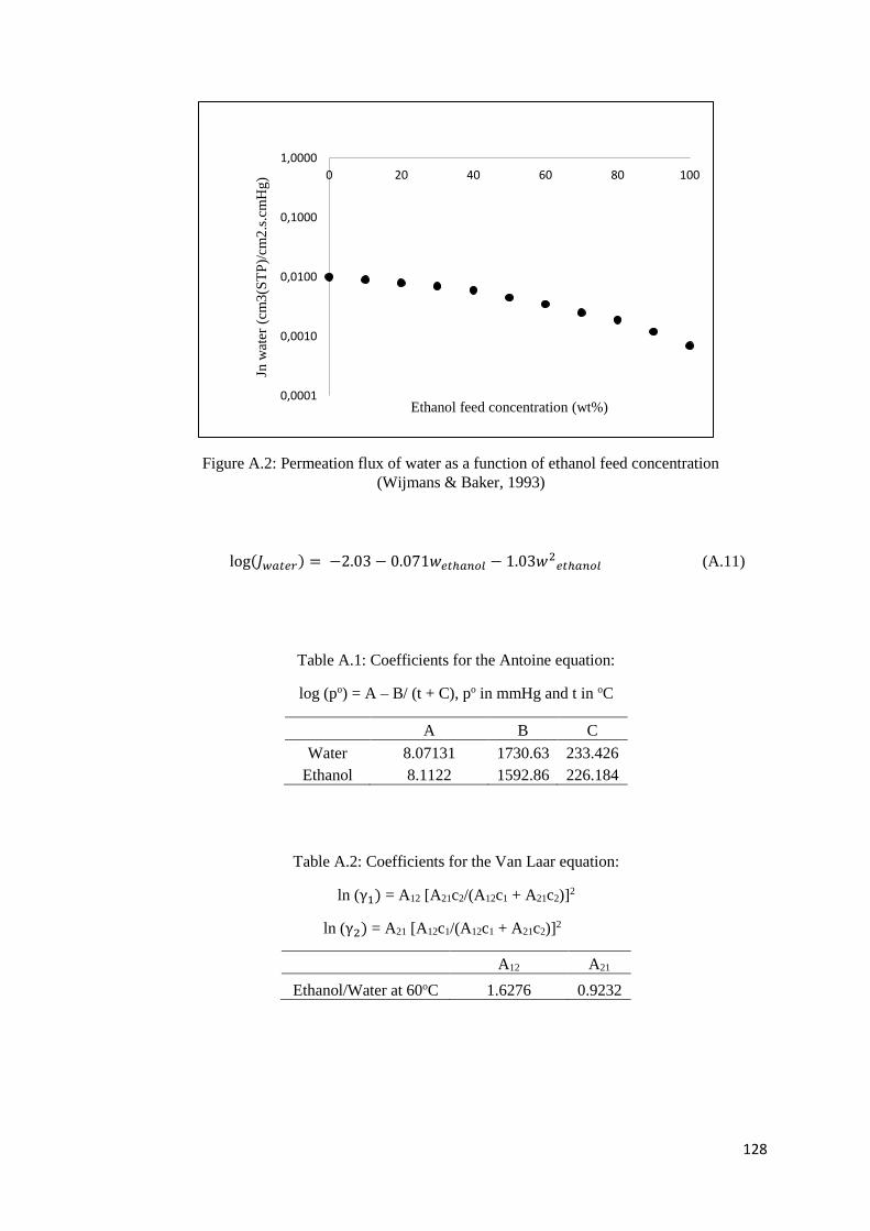
128

log(𝐽𝑤𝑎𝑡𝑒𝑟) = −2.03 − 0.071𝑤𝑒𝑡ℎ𝑎𝑛𝑜𝑙 − 1.03𝑤2𝑒𝑡ℎ𝑎𝑛𝑜𝑙 (A.11)

Table A.1: Coefficients for the Antoine equation:

log (po) = A – B/ (t + C), po in mmHg and t in oC

A B C

Water 8.07131 1730.63 233.426

Ethanol 8.1122 1592.86 226.184

Table A.2: Coefficients for the Van Laar equation:

ln (γ1) = A12 [A21c2/(A12c1 + A21c2)]2

ln (γ2) = A21 [A12c1/(A12c1 + A21c2)]2

A12 A21

Ethanol/Water at 60oC 1.6276 0.9232

0,0001

0,0010

0,0100

0,1000

1,0000

0 20 40 60 80 100

Jn w

ater

(cm

3(S

TP

)/cm

2.s

.cm

Hg)

Ethanol feed concentration (wt%)

Figure A.2: Permeation flux of water as a function of ethanol feed concentration

(Wijmans & Baker, 1993)

129

APPENDIX B: DETAILED COSTING PROCEDURE

B.1: Capital Investment Cost of Membrane and Module

The capital investment cost of the membrane and modules were calculated manually on Microsoft

Excel. This involved multiplying the membrane/module area by the literature costs shown in

Table B.1. The total membrane/module area required was calculated using the methodology by

Wijmans & Baker (1993) shown in appendix A. The capital investment cost of all other units

were evaluated using the Aspen Plus® computer software.

Table B.1: Literature cost of membrane and module

Polyvinyl alcohol Membrane 200 US Dollar/m2 (Kaewkannetra, et al., 2012)

Spiral Wound Module 100 US Dollar/m2 (Safobeen, 2011)

B.2: Operating Costs

The operating costs were determined by means of the utility prices displayed in Table B.2.

Table B.2: Utility costs

Utility Description Unit Price

Electricity (Jobson, 2014) Pound/kW.hr 0.08

Cooling water (Lladosa, et al., 2011) Euro/m3 0.04

Low pressure steam (Safobeen, 2011) USD/1000 kg steam 7

Medium pressure steam (Ocic, 2012) USD/1000 kg steam 9.66

High pressure steam (Ocic, 2012) USD/1000 kg steam 10.83

Liquid nitrogen (Safobeen, 2011) USD/litre 0.1

Ethylene glycol (TradeKey, 2016) USD/1000 kg steam 650

Membrane replacement (Van Hoof, et al., 2004) Euro/m2 550

As can be seen from Table B.2, the utility prices obtained from literature are in different

currencies and from different years. In order to present the final costs in a consistent form, the

currencies were converted into the South African rand via Table B.3 below. The prices were then

updated with the CEPCI (chemical engineering plant cost index) as shown in Table B.4 and

equation B.1.

130

Table B.3: Conversion of currencies to rands

Currency

South African Rand 1

Euro (The Money Converter, 2016) 14.45

US Dollar (The Money Converter, 2016) 12.93

British Pound (The Money Converter, 2016) 16.45

Table B.4: Chemical Engineering Plant Cost Index

Year CEPCI (Chemical Engineering Plant Cost

Index)

2004 (Chemical Engineering Online, 2008) 444.2





𝑅 (2016) = 𝑅 (𝑦𝑒𝑎𝑟) × 𝐶𝐸𝑃𝐶𝐼 (2016)

𝐶𝐸𝑃𝐶𝐼 (𝑦𝑒𝑎𝑟) (B.1)

The process utilities such as steam, cooling water and refrigerant were determined via equations

B.2 and B.3 below.

For Steam/Refrigerant : Q = m∆hvap (B.2)

For Cooling water : Q = mCp∆T (B.3)

Q : column duty (kW)

m : mass flow rate (kg/hr)

∆hvap: enthalpy of vaporisation (kJ/kg)

Cp : Heat capacity (kJ/kg.K)

∆T : temperature (K)

The duties are acquired from Aspen Plus®, the change in enthalpy of vaporisation and heat

capacities are obtained from the literature sources shown in Table B.5, the temperature change is

assumed to be 30 K. With this information, the mass flow rate of each utility can be calculated

and multiplied by the literature cost.

131

Table B.5: Enthalpy of vaporisation and heat capacities

Component ∆hvap (kJ/kg) Cp (kJ/kg.K)

Low Pressure Steam 2167.00 (Jobson, 2014) -

Medium Pressure Steam 2158.00 (Jobson, 2014) -

Cooling Water - 4.18 (Jobson, 2014)

Refrigerant (Nitrogen) 5592.80 (Safobeen, 2011) -

The duties of the pumps (feed and vacuum) are acquired from Aspen Plus®. The cost is obtained

by simply multiplying this value by the electricity cost from literature. The membrane

replacement is assumed to take place every five years. Hence this cost is divided by 5 and added

to the yearly process utility costs.

B.3: Inter-stage Heat Exchangers

For the inter-stage heat exchangers, the first step was to calculate the temperature drop between

each module. This was determined via equation B.4 (Schiffmann, 2014) and the values obtained

from Aspen Plus® shown in Table B.6.

∆𝑇 = 𝐹𝑝

𝐹𝑓 ×

∆ℎ𝑣𝑎𝑝,𝑤𝑎𝑡

𝑥𝑓,𝑒𝑡ℎ 𝐶𝑝𝑓,𝑒𝑡ℎ+ 𝑥𝑓,𝑤𝑎𝑡 𝐶𝑝𝑓,𝑤𝑎𝑡 (B.4)

Fp : Permeate flow rate

Ff : Feed flow rate

xf : mole fraction

Table B.6: Enthalpy of vaporisation and heat capacities from Aspen Plus®

Component ∆hvap (kJ/kmol) Cp (kJ/kmol.K)

Ethanol 136.58

Water 42515.7 77.11

This temperature change along with the retentate stream conditions from each module is then used

to calculate the heat duty. The process utility cost is there-after evaluated.

132

APPENDIX C: GAS CHROMATOGRAPH CALIBRATION

CHARTS

C.1 Test System: Ethanol (1) + Cyclohexane (4) System

Figure C.1: GC calibration for the ethanol (1) + cyclohexane (4) system in the more dilute


area.

Figure C.2: GC calibration for ethanol (1) + cyclohexane (4) system in the more dilute regions

of ethanol. Deviations in composition using a second order polynomial; where x1,TRUE is the

actual composition from the GC, and x1,CALC is the composition calculated from the calibration

polynomial.

y = -0,5472x2 + 2,2424x

R² = 0,9993

0

0,1

0,2

0,3

0,4

0,5

0,6

0,7

0,8

0,9

1

0,0 0,1 0,2 0,3 0,4 0,5

x1/x

4

A1/A4

-0,020

-0,015

-0,010

-0,005

0,000

0,005

0,010

0,0 0,1 0,2 0,3 0,4 0,5

x1

,CA

LC

-

x1,T

RU

E

x1,TRUE

133

Figure C.3: GC calibration for the ethanol (1) + cyclohexane (4) system in the more

concentrated regions of ethanol. Representation of the relationship between the number of

moles vs the peak area.

Figure C.4: GC calibration for the ethanol (1) + cyclohexane (4) system in the more

concentrated regions of ethanol. Deviations in composition using a second order polynomial;

where x1,TRUE is the actual composition from the GC, and x1,CALC is the composition calculated

from the calibration polynomial.

y = -0,0135x2 + 0,5383x

R² = 0,9992

0

0,1

0,2

0,3

0,4

0,5

0,6

0,7

0,8

0,9

1

0 0,2 0,4 0,6 0,8 1 1,2 1,4 1,6 1,8

x4/x

1

A4/A1

-0,006

-0,004

-0,002

0,000

0,002

0,004

0,006

0,008

0,5 0,6 0,7 0,8 0,9 1,0x1,C

AL

C-

x1,T

RU

E

x1. TRUE

134

C.2 Ethanol (1) + Pyridine (3) System

Figure C.5: GC calibration for the ethanol (1) + pyridine (3) system in the more dilute regions

of ethanol. Representation of the relationship between the number of moles vs the peak area.

Figure C.6: GC calibration for the ethanol (1) + pyridine (3) system in the more dilute regions

of ethanol. Deviations in composition using a second order polynomial; where x1,TRUE is the

actual composition from the GC, and x1,CALC is the composition calculated from the calibration

polynomial.

y = -0,1864x2 + 1,5072x

R² = 0,9997

0,0

0,2

0,4

0,6

0,8

1,0

0,0 0,1 0,2 0,3 0,4 0,5 0,6 0,7 0,8

x1/x

3

A1/A3

-0,008

-0,006

-0,004

-0,002

0,000

0,002

0,004

0,006

0,0 0,1 0,2 0,3 0,4 0,5 0,6

x1,C

AL

C -

x1,T

RU

E

x1,TRUE

135


regions of ethanol. Deviations in composition using a second order polynomial; where x1,TRUE is

the actual composition from the GC, and x1,CALC is the composition calculated from the

calibration polynomial.

y = -0,0100x2 + 0,7597x

R² = 0,9998

0

0,2

0,4

0,6

0,8

1

0 0,2 0,4 0,6 0,8 1 1,2 1,4 1,6

x3/x

1

A3/A1

-0,004

-0,003

-0,002

-0,001

0,000

0,001

0,002

0,003

0,004

0,005

0,006

0,007

0,4 0,5 0,6 0,7 0,8 0,9 1,0

x1,C

AL

C-

x1,T

RU

E

x1, TRUE

Figure C.7: GC calibration for the ethanol (1) + pyridine (3) system in the more

concentrated regions of ethanol. Representation of the relationship between the number of

moles vs the peak area.

136

C.3 Water (2) + Pyridine (3) System


water. Representation of the relationship between the number of moles vs the peak area.


water. Deviations in composition using a second order polynomial; where x2,TRUE is the actual

composition from the GC, and x2,CALC is the composition calculated from the calibration

polynomial.

y = -23,561x2 + 9,2386x

R² = 0,9969

0

0,1

0,2

0,3

0,4

0,5

0,6

0,7

0,8

0,9

1

0,00 0,05 0,10 0,15 0,20

x2/x

3

A2/A3

-0,020

-0,015

-0,010

-0,005

0,000

0,005

0,010

0,00 0,10 0,20 0,30 0,40 0,50

x2, C

AL

C -

x2, T

RU

E

x2, TRUE

137


regions of water. Representation of the relationship between the number of moles vs the peak

area.


regions of water. Deviations in composition using a second order polynomial; where x2,TRUE is

the actual composition from the GC, and x2,CALC is the composition calculated from the

calibration polynomial.

y = -0,0121x2 + 0,2789x

R² = 0,9999

0

0,1

0,2

0,3

0,4

0,5

0,6

0,7

0,8

0,9

1

0,00 0,50 1,00 1,50 2,00 2,50 3,00 3,50

x3/x

2

A3/A2

-0,0015

-0,0010

-0,0005

0,0000

0,0005

0,0010

0,0015

0,0020

0,0025

0,0030

0,0035

0,0040

0,5 0,6 0,7 0,8 0,9 1,0

x2,C

AL

C-

x2,T

RU

E

x2, TRUE

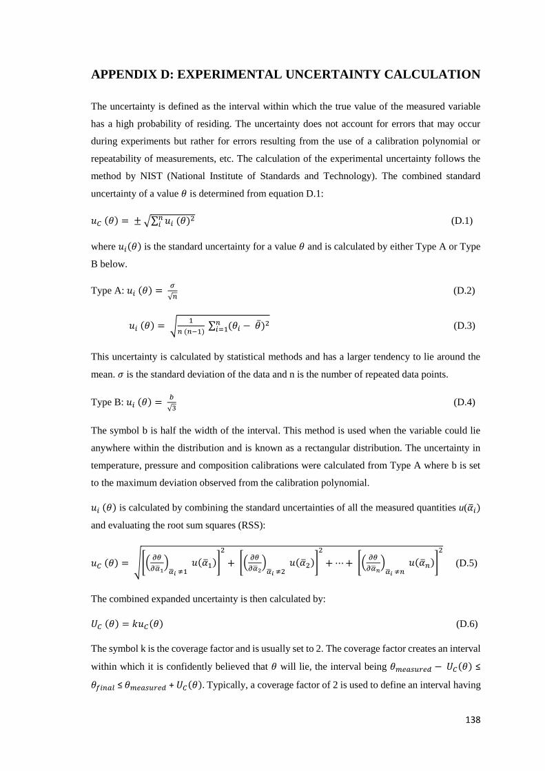
138

APPENDIX D: EXPERIMENTAL UNCERTAINTY CALCULATION

The uncertainty is defined as the interval within which the true value of the measured variable

has a high probability of residing. The uncertainty does not account for errors that may occur

during experiments but rather for errors resulting from the use of a calibration polynomial or

repeatability of measurements, etc. The calculation of the experimental uncertainty follows the

method by NIST (National Institute of Standards and Technology). The combined standard

uncertainty of a value 𝜃 is determined from equation D.1:

𝑢𝐶 (𝜃) = ± √∑ 𝑢𝑖 (𝜃)2𝑛

𝑖 (D.1)

where 𝑢𝑖(𝜃) is the standard uncertainty for a value 𝜃 and is calculated by either Type A or Type

B below.

Type A: 𝑢𝑖 (𝜃) = 𝜎

√𝑛 (D.2)

𝑢𝑖 (𝜃) = √1

𝑛 (𝑛−1) ∑ (𝜃𝑖 − �̅�)

2𝑛𝑖=1 (D.3)

This uncertainty is calculated by statistical methods and has a larger tendency to lie around the

mean. 𝜎 is the standard deviation of the data and n is the number of repeated data points.

Type B: 𝑢𝑖 (𝜃) = 𝑏

√3 (D.4)

The symbol b is half the width of the interval. This method is used when the variable could lie

anywhere within the distribution and is known as a rectangular distribution. The uncertainty in

temperature, pressure and composition calibrations were calculated from Type A where b is set

to the maximum deviation observed from the calibration polynomial.

𝑢𝑖 (𝜃) is calculated by combining the standard uncertainties of all the measured quantities u(�̅�𝑖)

and evaluating the root sum squares (RSS):

𝑢𝐶 (𝜃) = √[(𝜕𝜃

𝜕�̅�1)�̅�𝑖 ≠1

𝑢(�̅�1)]

2

+ [(

𝜕𝜃

𝜕�̅�2)�̅�𝑖 ≠2

𝑢(�̅�2)]

2

+ ⋯+ [(

𝜕𝜃

𝜕�̅�𝑛)�̅�𝑖 ≠𝑛

𝑢(�̅�𝑛)]

2

(D.5)

The combined expanded uncertainty is then calculated by:

𝑈𝐶 (𝜃) = 𝑘𝑢𝐶(𝜃) (D.6)

The symbol k is the coverage factor and is usually set to 2. The coverage factor creates an interval

within which it is confidently believed that 𝜃 will lie, the interval being 𝜃𝑚𝑒𝑎𝑠𝑢𝑟𝑒𝑑 − 𝑈𝐶(𝜃) ≤

𝜃𝑓𝑖𝑛𝑎𝑙 ≤ 𝜃𝑚𝑒𝑎𝑠𝑢𝑟𝑒𝑑 + 𝑈𝐶(𝜃). Typically, a coverage factor of 2 is used to define an interval having

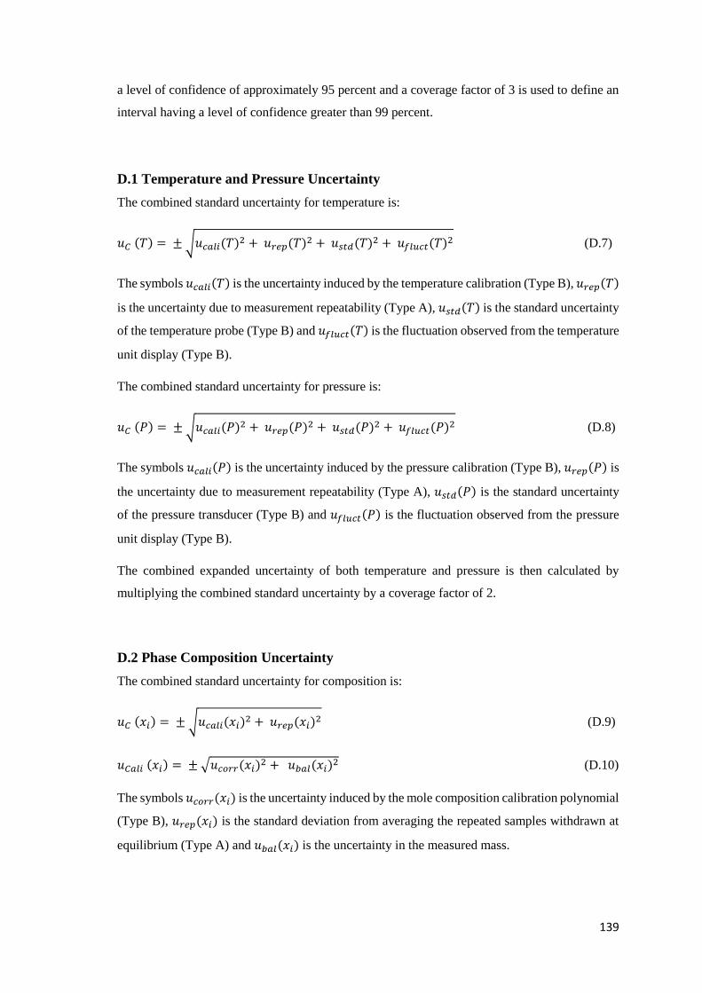
139

a level of confidence of approximately 95 percent and a coverage factor of 3 is used to define an

interval having a level of confidence greater than 99 percent.

D.1 Temperature and Pressure Uncertainty

The combined standard uncertainty for temperature is:

𝑢𝐶 (𝑇) = ± √𝑢𝑐𝑎𝑙𝑖(𝑇)2 + 𝑢𝑟𝑒𝑝(𝑇)

2 + 𝑢𝑠𝑡𝑑(𝑇)2 + 𝑢𝑓𝑙𝑢𝑐𝑡(𝑇)

2 (D.7)

The symbols 𝑢𝑐𝑎𝑙𝑖(𝑇) is the uncertainty induced by the temperature calibration (Type B), 𝑢𝑟𝑒𝑝(𝑇)

is the uncertainty due to measurement repeatability (Type A), 𝑢𝑠𝑡𝑑(𝑇) is the standard uncertainty

of the temperature probe (Type B) and 𝑢𝑓𝑙𝑢𝑐𝑡(𝑇) is the fluctuation observed from the temperature

unit display (Type B).

The combined standard uncertainty for pressure is:

𝑢𝐶 (𝑃) = ± √𝑢𝑐𝑎𝑙𝑖(𝑃)2 + 𝑢𝑟𝑒𝑝(𝑃)

2 + 𝑢𝑠𝑡𝑑(𝑃)2 + 𝑢𝑓𝑙𝑢𝑐𝑡(𝑃)

2 (D.8)

The symbols 𝑢𝑐𝑎𝑙𝑖(𝑃) is the uncertainty induced by the pressure calibration (Type B), 𝑢𝑟𝑒𝑝(𝑃) is

the uncertainty due to measurement repeatability (Type A), 𝑢𝑠𝑡𝑑(𝑃) is the standard uncertainty

of the pressure transducer (Type B) and 𝑢𝑓𝑙𝑢𝑐𝑡(𝑃) is the fluctuation observed from the pressure

unit display (Type B).

The combined expanded uncertainty of both temperature and pressure is then calculated by

multiplying the combined standard uncertainty by a coverage factor of 2.

D.2 Phase Composition Uncertainty

The combined standard uncertainty for composition is:

𝑢𝐶 (𝑥𝑖) = ± √𝑢𝑐𝑎𝑙𝑖(𝑥𝑖)2 + 𝑢𝑟𝑒𝑝(𝑥𝑖)

2 (D.9)

𝑢𝐶𝑎𝑙𝑖 (𝑥𝑖) = ± √𝑢𝑐𝑜𝑟𝑟(𝑥𝑖)2 + 𝑢𝑏𝑎𝑙(𝑥𝑖)

2 (D.10)

The symbols 𝑢𝑐𝑜𝑟𝑟(𝑥𝑖) is the uncertainty induced by the mole composition calibration polynomial

(Type B), 𝑢𝑟𝑒𝑝(𝑥𝑖) is the standard deviation from averaging the repeated samples withdrawn at

equilibrium (Type A) and 𝑢𝑏𝑎𝑙(𝑥𝑖) is the uncertainty in the measured mass.

140

Since 𝑥𝑖 is dependent on the meaurement of the masses mi and mj:

𝑢𝑏𝑎𝑙 (𝑥𝑖) = √[(𝜕𝑥𝑖

𝜕𝑚𝑖)𝑚𝑗

𝑢(𝑚𝑖)]

2

+ [(𝜕𝑥𝑖

𝜕𝑚𝑗)𝑚𝑖

𝑢(𝑚𝑗)]

2

(D.11)

using the defintion 𝑥𝑖 = 𝑛𝑖/(𝑛𝑖 + 𝑛𝑗) and 𝑛𝑖 = 𝑚𝑖/𝑀𝑀𝑖 where MM is the molecular mass,

equation B.11 can be simplified to:

𝑢𝑏𝑎𝑙 (𝑥𝑖) = 𝑥𝑖 𝑥𝑗√(𝑢(𝑚𝑖)

𝑚𝑖)2

+ (

𝑢(𝑚𝑗)

𝑚𝑗)2

(D.12)

however 𝑢𝑏𝑎𝑙 (𝑥𝑖) is neglected since 𝑢𝑐𝑜𝑟𝑟 (𝑥𝑖) >> 𝑢𝑏𝑎𝑙 (𝑥𝑖).

141

APPENDIX E: SENSITIVITY ANALYSIS PLOTS

E.1 Process 1FE (1 flash, extractive distillation):

Solvent Recovery Column (C-03)

Table E.1: Variation of feed stage location with reflux ratio

NoS FS RR

30 11 2.72

30 12 2.63

30 13 2.65

Figure E.1: Influence of number of stages on the total annual cost

Figure E.2: Influence of feed entry stage on the total annual cost at 32 stages

7,60E+05

7,62E+05

7,64E+05

7,66E+05

7,68E+05

7,70E+05

7,72E+05

30 31 32 33 34 35 36 37 38

TA

C (

US

D)

Number of Stages

7,55E+05

7,60E+05

7,65E+05

7,70E+05

7,75E+05

7,80E+05

7,85E+05

7,90E+05

7,95E+05

11 12 13 14

TA

C (

US

D)

Feed Stage

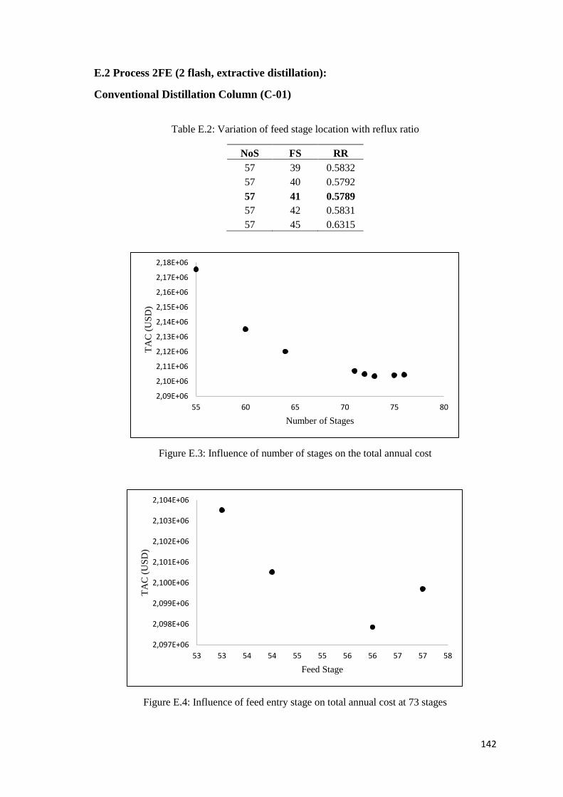
142

E.2 Process 2FE (2 flash, extractive distillation):



NoS FS RR

57 39 0.5832

57 40 0.5792

57 41 0.5789

57 42 0.5831

57 45 0.6315


Figure E.4: Influence of feed entry stage on total annual cost at 73 stages

2,09E+06

2,10E+06

2,11E+06

2,12E+06

2,13E+06

2,14E+06

2,15E+06

2,16E+06

2,17E+06

2,18E+06

55 60 65 70 75 80

TA

C (

US

D)

Number of Stages

2,097E+06

2,098E+06

2,099E+06

2,100E+06

2,101E+06

2,102E+06

2,103E+06

2,104E+06

53 53 54 54 55 55 56 56 57 57 58

TA

C (

US

D)

Feed Stage

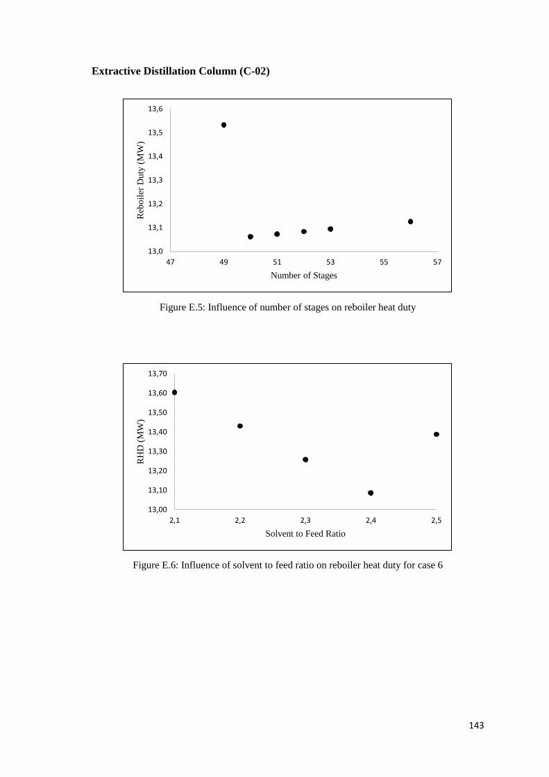
143

Extractive Distillation Column (C-02)

Figure E.5: Influence of number of stages on reboiler heat duty

Figure E.6: Influence of solvent to feed ratio on reboiler heat duty for case 6

13,0

13,1

13,2

13,3

13,4

13,5

13,6

47 49 51 53 55 57

Reb

oil

er D

uty

(M

W)

Number of Stages

13,00

13,10

13,20

13,30

13,40

13,50

13,60

13,70

2,1 2,2 2,3 2,4 2,5

RH

D (

MW

)

Solvent to Feed Ratio

144

Table E.3: Extractive distillation column specifications for each case

Case NoS FS SFS RR S/F Ratio Purity Recovery RHD (MW)

1 49 39 8 0.6 2.3 0.9998 0.9998 13.18

2 50 39 9 0.6 2.2 0.9998 0.9998 12.89

3 51 38 9 0.6 2.2 0.9998 0.9998 12.90

4 52 38 9 0.6 2.2 0.9998 0.9998 12.91

5 53 37 9 0.5 2.4 0.9998 0.9998 13.05

6 56 37 9 0.5 2.4 0.9998 0.9998 13.09

Figure E.7: Total annual cost for the different cases in the extractive distillation column

3,78E+06

3,80E+06

3,82E+06

3,84E+06

3,86E+06

3,88E+06

3,90E+06

3,92E+06

3,94E+06

3,96E+06

1 2 3 4 5 6

TA

C (

US

D)

Case

145

Solvent Recovery Column (C-03)


NoS FS RR

28 10 3.75

28 12 2.67

28 13 2.73


Figure E.9: Influence of feed entry stage on total annual cost at 33 stages

7,64E+05

7,65E+05

7,66E+05

7,67E+05

7,68E+05

7,69E+05

7,70E+05

7,71E+05

7,72E+05

25 27 29 31 33 35 37

TA

C (

US

D)

Number of Stages

7,61E+05

7,62E+05

7,63E+05

7,64E+05

7,65E+05

7,66E+05

7,67E+05

7,68E+05

7,69E+05

7,70E+05

7,71E+05

7,72E+05

12 13 14 15

TA

C (

US

D)

Feed Stage

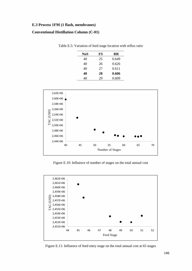
146

E.3 Process 1FM (1 flash, membranes)



NoS FS RR

40 25 0.649

40 26 0.626

40 27 0.611

40 28 0.606

40 29 0.609


Figure E.11: Influence of feed entry stage on the total annual cost at 65 stages

2,44E+06

2,46E+06

2,48E+06

2,50E+06

2,52E+06

2,54E+06

2,56E+06

2,58E+06

2,60E+06

2,62E+06

40 45 50 55 60 65 70

TA

C (

US

D)

Number of Stages

2,451E+06

2,452E+06

2,453E+06

2,454E+06

2,455E+06

2,456E+06

2,457E+06

2,458E+06

2,459E+06

2,460E+06

2,461E+06

2,462E+06

44 45 46 47 48 49 50 51 52

TA

C (

US

D)

Feed Stage

147

E.4 Process 2FM (2 flash, membranes)



NoS FS RR

40 25 0.654

40 26 0.624

40 27 0.609

40 28 0.604

40 29 0.608


Figure E.13: Influence on feed entry stage on the total annual cost at 63 stages

2,44E+06

2,46E+06

2,48E+06

2,50E+06

2,52E+06

2,54E+06

2,56E+06

2,58E+06

2,60E+06

2,62E+06

40 45 50 55 60 65 70

TA

C (

US

D)

Number of Stages

2,450E+06

2,452E+06

2,454E+06

2,456E+06

2,458E+06

2,460E+06

2,462E+06

2,464E+06

42 43 44 45 46 47 48 49 50

TA

C (

US

D)

Feed Stage

Separation and Recovery of a Complexing Agent in the ...

Documents

Transcript of Separation and Recovery of a Complexing Agent in the ...