Separating methane production and consumption with … · Separating methane production and...

Separating methane production and consumption with a field-based

isotope pool dilution technique

Joseph C. von Fischer1 and Lars O. Hedin2

Department of Ecology and Evolutionary Biology, Cornell University, Ithaca, New York, USA

Received 7 June 2001; revised 26 February 2002; accepted 26 February 2002; published 12 July 2002.

[1] Despite the importance of methane for climate, it has remained difficult to measuregross rates of methane production and consumption without inducing artifacts. To remedythis, we have developed, tested, and applied a field-based 13CH4 pool dilution technique.Laboratory tests, sensitivity analyses, and field data indicate that this technique is robustfor measuring gross rates of methane production and consumption. In our analyses of 130soil cores from 17 field sites of differing environmental conditions, we encountered awide range of gross methane production rates (0.04–930 mg CH4-C m�2 day�1), butencountered a narrower range of consumption rates (0.1–9.2 mg CH4-C m�2 day�1).Unexpectedly, we found that gross production of methane was common (mean = 0.15 mgCH4-C m�2 day�1) even in dry, oxic soils where average soil conditions cannot supportmethane producers. Through improved measurement of methane turnover in soils, thistechnique can offer a more fine-grained understanding of how productive andconsumptive processes are linked to soil-atmosphere trace gas balances. INDEX TERMS:

0315 Atmospheric Composition and Structure: Biosphere/atmosphere interactions; 1615 Global Change:

Biogeochemical processes (4805); 1694 Global Change: Instruments and techniques; 4840 Oceanography:

Biological and Chemical: Microbiology; KEYWORDS: methanogenesis, methanotrophy, isotope pool dilution,

anaerobic microsite, soil biogeochemistry, trace gas flux

1. Introduction

[2] Methane is a powerful heat-trapping gas that affectsthe Earth’s climate system [Wang et al., 1976; Cicerone andOremland, 1988; Harries et al., 2001]. Over the past400,000 years, atmospheric methane concentrations havegenerally risen in response to periods of warming, thusamplifying climate change [Petit et al., 1999] and raisingquestions about potential feedback mechanisms between thebiosphere and climate. Over the past 150 years, humanshave doubled the concentration of atmospheric methane[Etheridge et al., 1992], primarily through effects on theproduction of methane within soils and sediments [Ciceroneand Oremland, 1988; Lelieveld et al., 1998]. This modernrise is expected to contribute increasingly to anthropogenicclimate change [Houghton et al., 1996; Hansen et al.,1998], further underscoring the need to understand theprocesses that regulate atmospheric methane concentration.[3] A fundamental and remaining challenge lies in under-

standing the controls of gross methane production and con-sumption in soils [e.g., Cicerone and Oremland, 1988;Matthews, 2000; Matthews and Fung, 1987; Potter et al.,

1996; Potter, 1997;Walter and Heimann, 2000]. The balancebetween gross rates of production and consumption deter-mines whether a soil is a net source or sink for atmosphericmethane. Waterlogged soils are environments where produc-tion often exceeds consumption, accounting for 38% ofmodern net methane sources and accounting for 68% ofpreindustrial sources [Lelieveld et al., 1998]. In contrast,well-drained soils generally display net consumption ofmethane and create a small sink globally for atmosphericmethane [Lelieveld et al., 1998]. Changes in soil watercontent due to climate variations may therefore cause dra-matic (and potentially nonlinear) changes in methane emis-sions to the atmosphere [Matthews, 2000]. These changes, inturn, create feedbacks that depend on how soil methanetransformations respond to changes in soil moisture.[4] It is important to understand gross methane produc-

tion and consumption separately, because the microbialpopulations responsible for the two processes are ecologi-cally and evolutionarily very different, and they respondquite differently to environmental controls [Zinder, 1993;Hanson and Hanson, 1996; King, 1997]. Methane produc-tion and consumption are typically measured separately byinhibiting one process with chemical inhibitors or bymanipulating the soil oxygen status and thus the balancebetween productive and consumptive processes [e.g., Orem-land and Culbertson, 1992a, 1992b; Davidson and Schimel,1995; Yavitt et al., 1995; King, 1996; Saarnio et al., 1997;Moosavi and Crill, 1998]. However, such inhibitionapproaches provide only limited understanding of these

GLOBAL BIOGEOCHEMICAL CYCLES, VOL. 16, NO. 3, 10.1029/2001GB001448, 2002

1Now at Department of Geosciences, Princeton University, Princeton,New Jersey, USA.

2Now at Department of Ecology and Evolutionary Biology andPrinceton Environmental Institute, Princeton University, Princeton, NewJersey, USA.

Copyright 2002 by the American Geophysical Union.0886-6236/02/2001GB001448$12.00

8 - 1

processes, because chemical inhibitors can simultaneouslyaffect both processes [Frenzel, 1996; King, 1996] andbecause the manipulation of oxygen status relies on physicalor chemical disruption of the soil-microbe system [Madsen,1998; Sundh et al., 1994].[5] To date, techniques that do not involve inhibition have

relied on the addition of radiocarbon [e.g., Yavitt et al., 1990;Whalen et al., 1992; Andersen et al., 1998] or interpretationof patterns in the natural abundance of stable isotopes [e.g.,Chanton et al., 1997; Liptay et al., 1998; Sugimoto et al.,1998]. Unfortunately, radiocarbon techniques can only beused in the laboratory (but seeWieder and Yavitt [1994] for arare exception) and are thus subject to time delays betweenfield sampling and analysis and to disturbance to the soilsduring transport [Madsen, 1998; Sundh et al., 1994]. Naturalabundance stable isotope approaches are indirect and highlysensitive to assumptions of methane transport, isotopicfractionation effects, and isotopic signatures of source meth-ane [Snover and Quay, 2000].[6] Although these techniques have contributed to the

general understanding of methane production and consump-tion, more specific understanding of the soil-microbe sys-tem will depend on techniques that can more clearlyseparate productive and consumptive processes in the field.To this end, we have developed a new technique thatpermits simultaneous observations of methane productionand consumption in the field, based on the approach ofstable isotope pool dilution. In this paper, we develop amathematical model for determining rates of microbialactivity from measured mass and isotope data. We usecomputer simulations and field trials on different soil typesto examine the sensitivity of the technique to error inassumptions and analysis. Finally, we examine results fromfield application of the technique and discuss implicationsof our method for improved understanding of controls onmethane flux and soil microbial ecology.

2. Principles and Mathematical Model

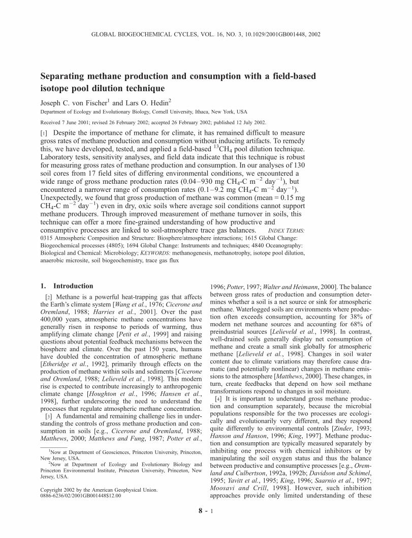
[7] Our technique is based on the principles of isotopepool dilution [Kirkham and Bartholomew, 1954, 1955],which we have adapted to study gross methane productionand consumption in soils using trace-level additions ofisotopically labeled methane. Here we develop an idealizedmodel assuming a closed system of soil particles andatmosphere where all methane exists in the atmosphericpool, as depicted in Figure 1. The approach depends onmeasuring changes in the amount of atmospheric methaneand the ratio of labeled to unlabeled methane over thecourse of the soil incubation. From these measured datawe can calculate gross methane consumption from the lossof labeled methane over time because, after an initialdiffusive redistribution of the added label [Andersen et al.,1998], only consumption affects this amount. Becauseproduction generates only unlabeled methane, we canfurther calculate gross methane production from the dilutionof labeled methane over time (i.e., isotope dilution). In thefollowing sections, we (1) describe the equations forchanges in the amount of unlabeled methane over time (2)describe the equation for changes in the amount of labeledmethane over time, and (3) describe the equation for change

in the ratio of labeled to unlabeled methane over time. Welater examine the sensitivity of this idealized model tovarious assumptions and to potential errors associated withfield-based measures.

2.1. Dynamics of Unlabeled Methane

[8] We assume that the amount of methane present in thesoil atmosphere (where the term ‘‘amount’’ refers to thenumber of moles of CH4 in the closed system) is influencedsolely by methane production and consumption. The bal-ance between these two processes ultimately determines thenet flux of methane between the soil and the atmosphere,described as

F ¼ P � C; ð1Þ

where F is the net flux rate between the soil and theatmosphere (e.g., in units of moles per hour), P is the grossrate of methane production, and C is the gross rate ofmethane consumption.[9] In the incubation chamber, methane concentrations

can be expected to rise or fall over time in response to thebalance between methane production and consumption.Because methane consumption follows Michaelis-Mentenkinetics [Bender and Conrad, 1992; Roslev et al., 1997], wecan expect the rate of consumption to change with anychanges in methane concentration over the course of theincubation. Atmospheric methane concentrations are typi-

Figure 1. Conceptual diagram of pool dilution approachfor measuring gross methane production and consumptionusing additions of labeled methane molecules (i.e., 13CH4)in a closed system. (a) Simultaneous processes of methaneproduction and consumption that affect total amount ofmethane. We describe the methane production rate, P, asconstant and describe the methane consumption rate as theproduct of a first-order rate constant, k, and the amount ofmethane, m. (b) Illustration showing that only methaneconsumption affects the amount of label, n. Isotopicfractionation slows consumption of label by a constantamount, a. See section 2 for a more detailed treatment ofthese relationships.

8 - 2 VON FISCHER AND HEDIN: METHANE ISOTOPE POOL DILUTION

cally below the Km, so we can use a first-order relationshipto model consumption [Fenchel et al., 1998; King, 1997;Roslev et al., 1997]. Thus

Ct ¼ kmt; ð2Þ

where Ct is the instantaneous rate of methane consumptionat time t, k is the first-order rate constant for consumption,and mt is the amount of methane at time t. Because thenumber of moles is equivalent to concentration in a closedsystem of constant volume, we have modeled consumptionin equation (2) as a first-order reaction with respect to theamount of methane, thus simplifying subsequent equations.The consumption constant, k, can be used to calculate theconsumption rate at a particular methane concentration, b,(e.g., in units of microliters per liter) if k is corrected for thevolume of the incubation container, v, and by the concen-tration of interest. Then

C ¼ bkv: ð3ÞUnder most conditions, we can assume the methaneconcentration over the soil surface is equal to the atmosphericconcentration of 1.8 mL L�1, so the gross consumption rate iscalculated for b = 1.8 mL L�1. Our formulation designates theatmospheric methane pool as the point of reference formeasuring gross rates of methane production and consump-tion. Thus the derived constants (i.e., P, C, and k) reflectexchanges across the soil-atmosphere boundary, with thelocation of source/sink region defined empirically by thedepth of label penetration into the soil.[10] The consumption rate in equations (2) and (3) is

expressed as a function of m and k. As a result, k incorpo-rates environmental constraints, including oxygen limitationand other factors. Even though methane consumption mightbe a function of oxygen concentration at low oxygenconditions, (i.e., C = kO2) rather than a function of methaneconcentration (i.e., C = kCH4), the practical determinationof k according to equation (2) results in an empiricallydetermined coefficient that incorporates effects due to bothmethane and oxygen.[11] We can now incorporate equation (2) into equation (1)

and represent instantaneous rates, like those in equation (2),as derivatives with respect to time:

F ¼ dm

dt¼ P � km: ð4Þ

The solution of equation (4) is

mt ¼P

k� P

k� m0

� �exp ð�ktÞ; ð5Þ

where m0 is the initial mass of methane. The solution, mt,describes how the amount of methane changes over time.These changes in mass can take on one of three qualitatively

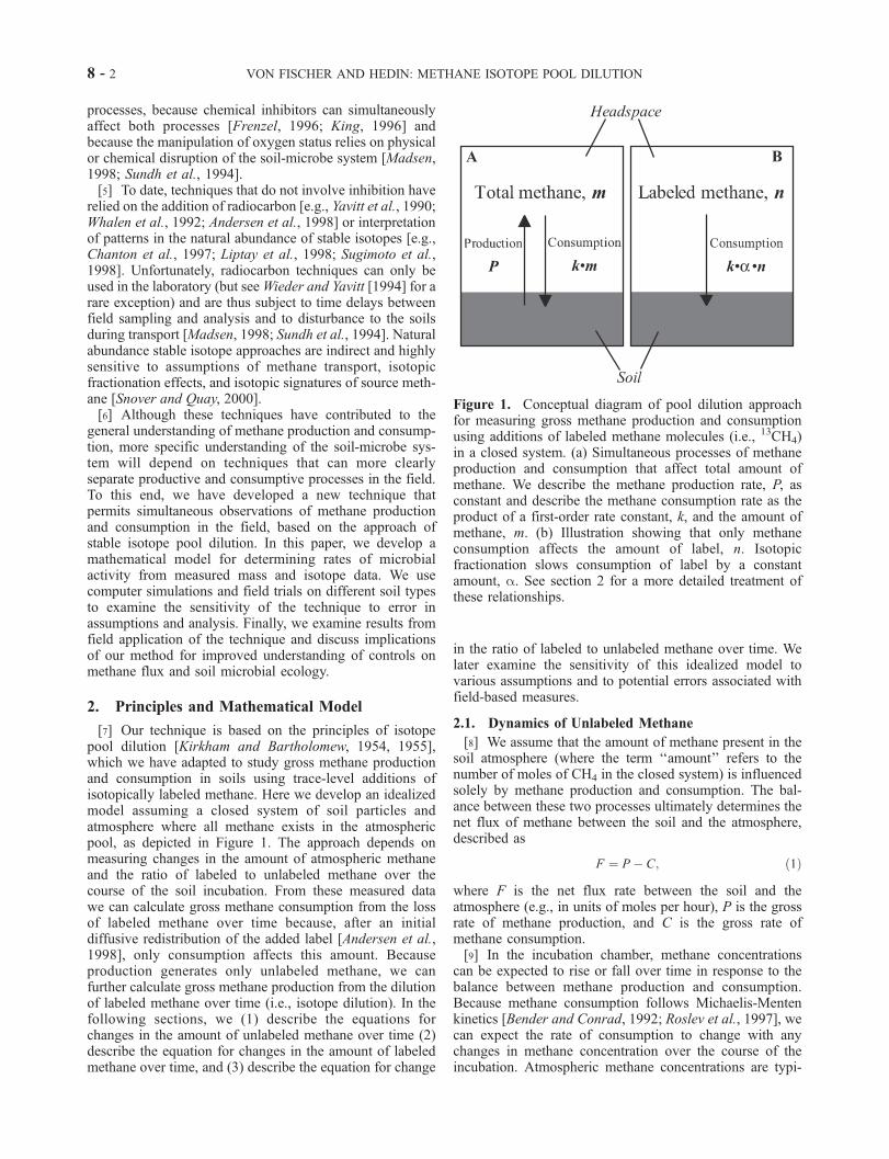
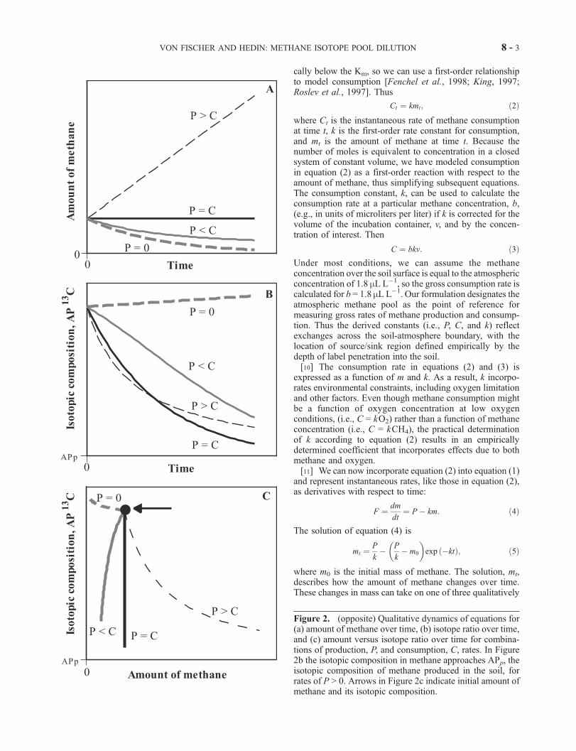
Figure 2. (opposite) Qualitative dynamics of equations for(a) amount of methane over time, (b) isotope ratio over time,and (c) amount versus isotope ratio over time for combina-tions of production, P, and consumption, C, rates. In Figure2b the isotopic composition in methane approaches APp, theisotopic composition of methane produced in the soil, forrates of P > 0. Arrows in Figure 2c indicate initial amount ofmethane and its isotopic composition.

VON FISCHER AND HEDIN: METHANE ISOTOPE POOL DILUTION 8 - 3

different dynamics (Figure 2a): increasing (P > C ), constant(P = C ), or decreasing (P < C, P = 0).[12] When both P and k are nonzero, the amount of

methane in the system reaches steady state when

m ¼ P

k: ð6Þ

This equilibrium point has been previously described forbiogenic trace gases as the ‘‘compensation concentration’’where productive and consumptive processes are balancedin the soil [Conrad, 1994].

2.2. Dynamics of Labeled Methane

[13] It is not possible to determine unique rates ofproduction and consumption by only following changes inthe amount of methane, because the single mass balanceequation (4) depends on two unknown variables, P and k.However, by coupling the mass balance equation with anexpression that describes how the ratio of labeled tounlabeled methane (i.e., the isotopic composition) changesover time, we are able to determine both P and k. While wedescribe the addition of 13C methane, our treatment can beapplied to other isotopes of methane like D/H or 14C/12C.[14] To uniquely follow the amount of 13C label over time,

we correct for any 13C generated by methane production bysubtracting the fixed isotopic composition of methane that isproduced. The amount of added 13C methane at time t can berelated to the percent abundance of 13C in total methane as

nt ¼ mt APt � APp

� �; ð7Þ

where nt is the amount of labeled methane, mt is the totalamount of methane, APt is the measured atom percent 13Cmethane in the system, and APp is the atom percent 13C ofmethane generated by methane production (see Appendix Afor conventions of reporting isotopic composition).[15] The equation used to model the total amount of

methane (equation (4)) can be simplified and applied toreflect the amount of the labeled methane, n, following twomodifications. First, because there is no production oflabeled methane during incubation, we can remove theproduction term, P, from equation (4). Second, isotopicfractionation slows the rate of consumption of 13C methaneby a very slight but constant amount, a, as compared tounlabeled methane, which is overwhelmingly 12CH4. Thefractionation coefficient follows the notation: a = k13/k12,where k12 is the first-order rate constant for consumption of12CH4 and k13 is the first-order rate constant for consump-tion of 13CH4. The resulting equation describes the instanta-neous change in the amount of label with respect to time as

dn

dt¼ �kan: ð8Þ

The solution to equation (8) describes how the mass of labelchanges over time:

nt ¼ n0 exp �katð Þ; ð9Þ

where n0 is the initial mass of labeled methane.[16] Having developed equations to describe the amount

of both labeled and unlabeled methane, it now becomes

straightforward to describe how the isotopic composition ofthe system changes with time. The amount of methane andits isotopic composition are the two properties in the head-space that are measured during the incubation, and theequation for isotopic composition is necessary for calculat-ing methane production.

2.3. Dynamics of Isotopic Composition

[17] We generate the equation for describing the isotopiccomposition over time by first rearranging equation (7) tothe form

APt ¼nt

mt

þ APp: ð10Þ

Then, by defining mt as in equation (5) and defining nt as inequation (9), we get

APt ¼n0 expð�katÞ

Pk� P

k� m0

� �expð�ktÞ

!þ APp: ð11Þ

[18] Equation (11) has two qualitatively different dynam-ics depending on the size of P with respect to C. When P isgreater than C, equation (11) predicts a decline in the atompercent 13C over time because production dilutes the labeledmethane. Figure 2b demonstrates this behavior where, astime approaches infinity, the isotopic composition of meth-ane, APt, approaches the isotopic composition of producedmethane, APp, for all cases except where P = 0. In general,the rate at which APt approaches APp is greater when thecombined rate of P and C (i.e., the turnover rate of themethane pool) is greater. When P is small as compared to C(illustrated for P = 0 in Figure 2b), methane in the systembecomes enriched in 13C, causing the isotope ratio to in-crease. This increase, known as a Rayleigh distillation[Hoefs, 1997], results from isotopic fractionation where theheavier isotope accumulates over time due to preferentialconsumption of 12CH relative to 13CH4.[19] We have expressed the changes in methane amount

and isotope ratio with respect to time (i.e., in equations (5)and (11),. However, the changes in amount can also beconsidered with respect to changes in the isotope ratio(Figure 2c) to observe the unique trajectory that is generatedby each combination of production and consumption rates.As we describe in section 2.4, we use the product ofmethane amount and isotope ratio (i.e., n in equation (7))to determine k, while we use the two measures separately(as in Figure 2c) to determine P.

2.4. Determination of Production and ConsumptionFrom Data

[20] The gross rates of methane production and consump-tion can be uniquely determined by fitting equations for theamount of labeled methane (equation (9)), the total amountof methane (equation (5) and the isotope ratio (equation (11))to measured data. Figure 3 illustrates these principal equa-tions and gives examples of their dynamics. We use a two-step process for fitting the equations to data. We firstdetermine the consumption rate constant, k, by linear regres-sion. Then we combine this value of k with measures of theamount of methane and its isotopic composition to determineP using a curve fitting routine.


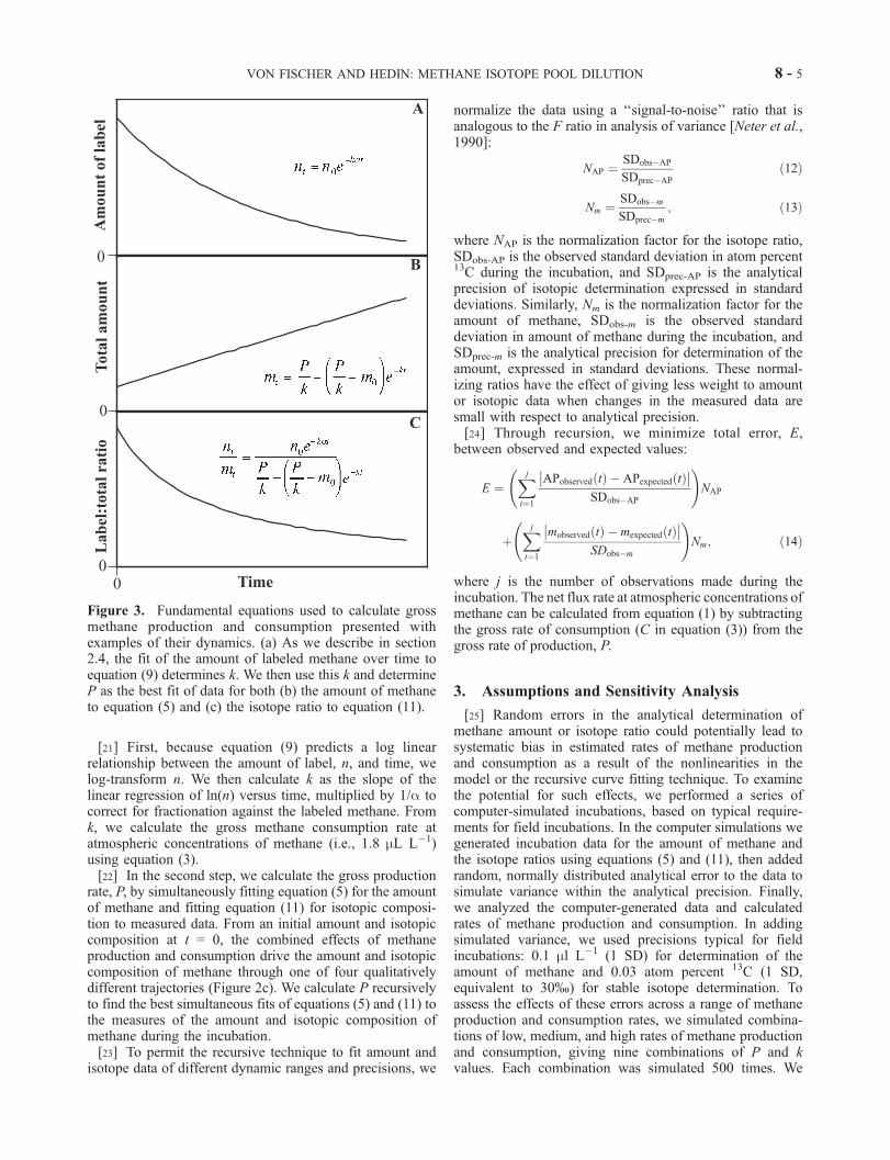
[21] First, because equation (9) predicts a log linearrelationship between the amount of label, n, and time, welog-transform n. We then calculate k as the slope of thelinear regression of ln(n) versus time, multiplied by 1/a tocorrect for fractionation against the labeled methane. Fromk, we calculate the gross methane consumption rate atatmospheric concentrations of methane (i.e., 1.8 mL L�1)using equation (3).[22] In the second step, we calculate the gross production

rate, P, by simultaneously fitting equation (5) for the amountof methane and fitting equation (11) for isotopic composi-tion to measured data. From an initial amount and isotopiccomposition at t = 0, the combined effects of methaneproduction and consumption drive the amount and isotopiccomposition of methane through one of four qualitativelydifferent trajectories (Figure 2c). We calculate P recursivelyto find the best simultaneous fits of equations (5) and (11) tothe measures of the amount and isotopic composition ofmethane during the incubation.[23] To permit the recursive technique to fit amount and

isotope data of different dynamic ranges and precisions, we

normalize the data using a ‘‘signal-to-noise’’ ratio that isanalogous to the F ratio in analysis of variance [Neter et al.,1990]:

NAP ¼ SDobs�AP

SDprec�AP

ð12Þ

Nm ¼ SDobs�m

SDprec�m

; ð13Þ

where NAP is the normalization factor for the isotope ratio,SDobs-AP is the observed standard deviation in atom percent13C during the incubation, and SDprec-AP is the analyticalprecision of isotopic determination expressed in standarddeviations. Similarly, Nm is the normalization factor for theamount of methane, SDobs-m is the observed standarddeviation in amount of methane during the incubation, andSDprec-m is the analytical precision for determination of theamount, expressed in standard deviations. These normal-izing ratios have the effect of giving less weight to amountor isotopic data when changes in the measured data aresmall with respect to analytical precision.[24] Through recursion, we minimize total error, E,

between observed and expected values:

E ¼Xjt¼1

APobserved tð Þ � APexpected tð Þ��

SDobs�AP

!NAP

þXjt¼1

mobserved tð Þ � mexpected tð Þ��

SDobs�m

!Nm; ð14Þ

where j is the number of observations made during theincubation. The net flux rate at atmospheric concentrations ofmethane can be calculated from equation (1) by subtractingthe gross rate of consumption (C in equation (3)) from thegross rate of production, P.

3. Assumptions and Sensitivity Analysis

[25] Random errors in the analytical determination ofmethane amount or isotope ratio could potentially lead tosystematic bias in estimated rates of methane productionand consumption as a result of the nonlinearities in themodel or the recursive curve fitting technique. To examinethe potential for such effects, we performed a series ofcomputer-simulated incubations, based on typical require-ments for field incubations. In the computer simulations wegenerated incubation data for the amount of methane andthe isotope ratios using equations (5) and (11), then addedrandom, normally distributed analytical error to the data tosimulate variance within the analytical precision. Finally,we analyzed the computer-generated data and calculatedrates of methane production and consumption. In addingsimulated variance, we used precisions typical for fieldincubations: 0.1 ml L�1 (1 SD) for determination of theamount of methane and 0.03 atom percent 13C (1 SD,equivalent to 30%) for stable isotope determination. Toassess the effects of these errors across a range of methaneproduction and consumption rates, we simulated combina-tions of low, medium, and high rates of methane productionand consumption, giving nine combinations of P and kvalues. Each combination was simulated 500 times. We

Figure 3. Fundamental equations used to calculate grossmethane production and consumption presented withexamples of their dynamics. (a) As we describe in section2.4, the fit of the amount of labeled methane over time toequation (9) determines k. We then use this k and determineP as the best fit of data for both (b) the amount of methaneto equation (5) and (c) the isotope ratio to equation (11).


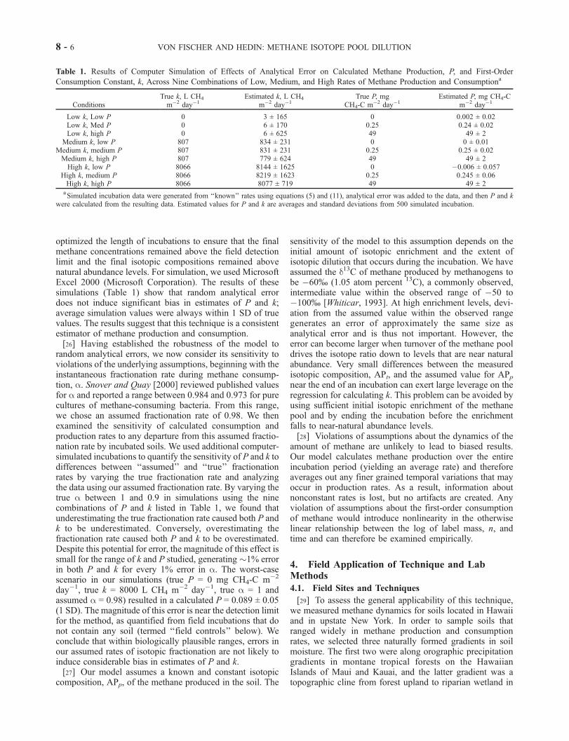
optimized the length of incubations to ensure that the finalmethane concentrations remained above the field detectionlimit and the final isotopic compositions remained abovenatural abundance levels. For simulation, we used MicrosoftExcel 2000 (Microsoft Corporation). The results of thesesimulations (Table 1) show that random analytical errordoes not induce significant bias in estimates of P and k;average simulation values were always within 1 SD of truevalues. The results suggest that this technique is a consistentestimator of methane production and consumption.[26] Having established the robustness of the model to

random analytical errors, we now consider its sensitivity toviolations of the underlying assumptions, beginning with theinstantaneous fractionation rate during methane consump-tion, a. Snover and Quay [2000] reviewed published valuesfor a and reported a range between 0.984 and 0.973 for purecultures of methane-consuming bacteria. From this range,we chose an assumed fractionation rate of 0.98. We thenexamined the sensitivity of calculated consumption andproduction rates to any departure from this assumed fractio-nation rate by incubated soils. We used additional computer-simulated incubations to quantify the sensitivity of P and k todifferences between ‘‘assumed’’ and ‘‘true’’ fractionationrates by varying the true fractionation rate and analyzingthe data using our assumed fractionation rate. By varying thetrue a between 1 and 0.9 in simulations using the ninecombinations of P and k listed in Table 1, we found thatunderestimating the true fractionation rate caused both P andk to be underestimated. Conversely, overestimating thefractionation rate caused both P and k to be overestimated.Despite this potential for error, the magnitude of this effect issmall for the range of k and P studied, generating �1% errorin both P and k for every 1% error in a. The worst-casescenario in our simulations (true P = 0 mg CH4-C m�2

day�1, true k = 8000 L CH4 m�2 day�1, true a = 1 andassumed a = 0.98) resulted in a calculated P = 0.089 ± 0.05(1 SD). The magnitude of this error is near the detection limitfor the method, as quantified from field incubations that donot contain any soil (termed ‘‘field controls’’ below). Weconclude that within biologically plausible ranges, errors inour assumed rates of isotopic fractionation are not likely toinduce considerable bias in estimates of P and k.[27] Our model assumes a known and constant isotopic

composition, APp, of the methane produced in the soil. The

sensitivity of the model to this assumption depends on theinitial amount of isotopic enrichment and the extent ofisotopic dilution that occurs during the incubation. We haveassumed the d13C of methane produced by methanogens tobe �60% (1.05 atom percent 13C), a commonly observed,intermediate value within the observed range of �50 to�100% [Whiticar, 1993]. At high enrichment levels, devi-ation from the assumed value within the observed rangegenerates an error of approximately the same size asanalytical error and is thus not important. However, theerror can become larger when turnover of the methane pooldrives the isotope ratio down to levels that are near naturalabundance. Very small differences between the measuredisotopic composition, APt, and the assumed value for APpnear the end of an incubation can exert large leverage on theregression for calculating k. This problem can be avoided byusing sufficient initial isotopic enrichment of the methanepool and by ending the incubation before the enrichmentfalls to near-natural abundance levels.[28] Violations of assumptions about the dynamics of the

amount of methane are unlikely to lead to biased results.Our model calculates methane production over the entireincubation period (yielding an average rate) and thereforeaverages out any finer grained temporal variations that mayoccur in production rates. As a result, information aboutnonconstant rates is lost, but no artifacts are created. Anyviolation of assumptions about the first-order consumptionof methane would introduce nonlinearity in the otherwiselinear relationship between the log of label mass, n, andtime and can therefore be examined empirically.

4. Field Application of Technique and LabMethods

4.1. Field Sites and Techniques

[29] To assess the general applicability of this technique,we measured methane dynamics for soils located in Hawaiiand in upstate New York. In order to sample soils thatranged widely in methane production and consumptionrates, we selected three naturally formed gradients in soilmoisture. The first two were along orographic precipitationgradients in montane tropical forests on the HawaiianIslands of Maui and Kauai, and the latter gradient was atopographic cline from forest upland to riparian wetland in

Table 1. Results of Computer Simulation of Effects of Analytical Error on Calculated Methane Production, P, and First-Order

Consumption Constant, k, Across Nine Combinations of Low, Medium, and High Rates of Methane Production and Consumptiona

ConditionsTrue k, L CH4

m�2 day�1Estimated k, L CH4

m�2 day�1True P, mg

CH4-C m�2 day�1Estimated P, mg CH4-C

m�2 day�1

Low k, Low P 0 3 ± 165 0 0.002 ± 0.02Low k, Med P 0 6 ± 170 0.25 0.24 ± 0.02Low k, high P 0 6 ± 625 49 49 ± 2

Medium k, low P 807 834 ± 231 0 0 ± 0.01Medium k, medium P 807 831 ± 231 0.25 0.25 ± 0.02Medium k, high P 807 779 ± 624 49 49 ± 2High k, low P 8066 8144 ± 1625 0 �0.006 ± 0.057

High k, medium P 8066 8219 ± 1623 0.25 0.245 ± 0.06High k, high P 8066 8077 ± 719 49 49 ± 2aSimulated incubation data were generated from ‘‘known’’ rates using equations (5) and (11), analytical error was added to the data, and then P and k

were calculated from the resulting data. Estimated values for P and k are averages and standard deviations from 500 simulated incubation.


New York State. Both the Maui and Kauai gradients aredominated by one of two native tree species: Acacia koa,which is only present in the drier two sites of each gradient,and Meterosideros polymorpha, which is present on mostsites in both gradients but dominant only on the wetter sites.Soils on both gradients are derived from volcanic shieldmaterial, �500,000 years old on the Maui gradient and�4,100,000 years old on the Kauai gradient. Soil carboncontent on these gradients ranges from 9% (weight/weightpercent) in the dry sites to 46% in the wet sites. We did notencounter standing water in any site along these gradients.Sites along the Maui gradient have been described in detailby Schuur et al. [2001].[30] The topographic cline in New York consisted of

mixed maple and oak (Acer spp., Quercus spp.) woodlandon the most well-drained site, sedge (Carex spp.) in theintermediate moisture sites, and an unvegetated streamsediment at the wet end. Soils in this part of New YorkState are derived from shale and are generally high in clay.Along this gradient, the soils increased in carbon contentwith soil moisture, from 4% in the upland to 33% in thewettest site. Standing water was only present on the wettestsite. In addition to this topographic gradient, we alsosampled two contrasting sites in a hemlock (Tsuga cana-densis) forest in New York State: one on well-drained andone on poorly drained soils. Like the other upstate NewYork sites, the soils at these hemlock sites were derivedfrom shale, but the mineral soils were overlain with a thickorganic horizon, >8 cm in the drier site and >30 cm in thewet site. At all sites in this study, we sampled soils wheresoil moisture was uniform with depth as opposed to soilswhere a well-drained horizon may overlay a waterloggedhorizon.[31] We performed short-term (3–6 hours) incubations of

intact soil cores at each site. We carefully collected undis-turbed soil samples of the top 10–15 cm of soil with a corerthat contained a plastic sleeve (15 cm deep, 5 cm diameter).Keeping the soil core within the sleeve, we then sealed thebottom end of the core with a plastic cap to eliminate gasexchange from soil surfaces that would not have beenexposed to the atmosphere. The soil was sealed into a1-quart canning jar to create a closed system for the13CH4 additions; the lid of the jar had been fitted with aport for gas sampling. We incubated soils immediately byburying the jar vertically in the soil near where the samplehad been taken. Temperature and light therefore remainedvery similar to original conditions.[32] We enriched the atmosphere in the incubation jar by

adding labeled methane at the beginning of the incubation.Our target was an isotopic enrichment of 2–10 atompercent 13C-methane. This addition led to a 2–10%increase in the headspace methane concentration so that,for example, a 5 atom percent addition to an incubation atatmospheric concentration would yield an increase from1.80 to 1.89 mL CH4 L�1. The isotopically enrichedmethane was diluted with air from 99% 13CH4 (Isotec,Inc.) prior to its addition to the incubation containers. Toensure even initial distribution of the label, we immedi-ately mixed the atmosphere of the incubation jar five timeswith a 60-mL syringe and left the incubation jar to

preincubate for 30–45 min so that the rapid, diffusiveredistribution of the isotope into the soil core would notbias our measures of isotope dynamics [see Andersen et al.,1998].[33] To adequately follow changes in methane mass and

isotopic composition over the course of the incubation, wecollected at least four samples: one sample after the pre-incubation (t = 0) and three samples spaced at roughly equalintervals throughout the remainder of the incubation. Typ-ical headspace volumes were �800 mL, while samplevolumes were 60 mL. We added a known volume ofultrahigh-purity helium to the incubation jar following eachsample removal to prevent any effects due to pressurevariations; all measures of methane concentrations werecorrected for this helium addition. Occasionally, samplesof either methane concentration or isotope ratio were lostdue to analytical or other errors. In such cases, no data wasused for that time point toward the calculation of methaneproduction and consumption rates.[34] Concurrent with each set of soil incubations, we

incubated a jar without a soil core as a field control to testfor leakage or any other effect not due to the soils. Thesecontrols also served as tests of analytical precision. Thevariance in measured amounts and isotope ratios of methanein these controls was used in the error calculation (equations(12) and (13)) for determining methane production rate. Totest for any abiotic soil effects on methane mass and isotoperatio, we also performed a laboratory experiment using soilsamples that had been autoclaved at 250�C for 90 min at apressure of 140 kPa.[35] We stored and transported gas samples in glass serum

vials with aluminum crimp tops, fitted with 20-mm butylrubber septa (Geomicrobial Inject Technologies, Oechelata,Oklahoma). Compared with other types of septa, we foundthat these exhibited minimum leakage and minimum blankcontamination. We divided each 60-mL gas sample from theincubation into two parts; 10 mL for gas chromatographicanalysis were compressed into 5-mL vials that had previ-ously been evacuated, and the remaining 50 mL werecompressed into 60-mL vials that had previously beenflushed with ultrahigh-purity helium. To account for thesmall amount of leakage and/or the presence of blanks thatcan arise from the storage and transport of samples, wefilled vials in the field with known standards and correctedthe concentration of the samples for any consistent changesin the standards. The correction for 5-mL vials typicallyincluded subtraction of a blank of �0.4 mL L�1 andaccounting for �7% leakage. The larger 60-mL vials usedfor isotopic analysis had trivial blanks and leakage, so nocorrection was applied. We analyzed the 5-mL vials formethane concentration within 1 week of sampling andanalyzed the 60-mL vials within 3 weeks.

4.2. Laboratory Techniques

[36] We determined the methane concentration by gaschromatography on an SRI 8610 with a Hayesep N columnor on a Varian 3400 cx with a Chromosorb 102 column.Typical standard deviations for repeated measurement ofstandard air was <0.1 mL L�1. Gas chromatographs werecalibrated by analyzing standards of at least three levels of


methane in triplicate and calculating the average instrumentresponse for each standard. No methane peak was everpresent in methane-free gases, so only the instrumentresponse (i.e., slope) was used. The detection limit formethane was 0.1 mL L�1, and all measured concentrationsbelow that limit are reported as 0.05 mL L�1.[37] Methane was prepared for isotopic analysis on a

highly modified Europa Scientific ANCA TG, similar tosystems described by Chanton et al. [1992] and Brand[1995]. In our system an air sample was manually intro-duced and carried by ultrahigh-purity helium under apressure of 120 kPa. The gas stream passed through achemical and a cryogenic trap to remove water vapor,carbon dioxide, and carbon monoxide: Mg(ClO4)2removed water vapor, Schutze Reagent (LECO Corpora-tion) oxidized CO to CO2, Carbosorb (a NaOH-basedcompound, PDZ Europa) removed CO2, and a liquidnitrogen trap removed any remaining CO2 water vaporand other condensable gases. Following purification thesample methane was oxidized to CO2 in an oven at1050�C over a nickel and platinum catalyst. Water pro-duced during combustion was removed in an isopropanol-dry ice mixture cryogenic trap maintained at �40�C ±5�C. The sample CO2 was cryofocused in a coil of nickeltubing immersed in liquid nitrogen and was subsequentlytransferred to the mass spectrometer, where an open splitadmitted a fraction of the sample CO2 to the ion source.Isotopic analysis was performed on a Europa ScientificGeo 20–20 stable isotope ratio mass spectrometer (PDZEuropa) calibrated to a working standard of air containing2 mL L�1 methane (4.5 nmol CH4 per 50 mL sample),d13C = �40.95% as calibrated from the natural gasstandard (NGS1). Typical analytical reproducibility ofstandards was ±1% (1 SD).[38] We evaluated performance of the mass spectrometer

and inlet system in several different ways. Most importantly,we observed no effect of contaminants or of changingsample size on the measured isotope ratio of methane.Injection of ultrahigh-purity helium produced very smallsystem blanks, typically �0.2 nmol. Samples were correctedfor this blank. Experimentally elevated concentrations ofcarbon dioxide, an important potential contaminant, did notaffect the isotope ratio of standards. Replicate samples of aircontaining ambient CO2 (�355 ppm, d13C of CO2 approx-imately �7%) and elevated CO2 (33,000 ppm, d13C ofCO2 �0%) had no effect on the measured d13C of CH4-C( p > 0.4, n = 2). Typically, there was very little carryoverfrom one sample to the next, and the carryover affectedonly samples of vastly different mass and isotopic com-position. We avoided side-by-side analyses of such differ-ent samples and applied an empirically determinedcarryover rate that was typically �0.5%. Although isotoperatios may vary as a function of sample size in some massspectrometer systems (N. Ostrom and S. Prossor, personalcommunication, 1998), we observed no effect >5% across10� variation in sample mass in our frequent tests of suchlinearity.[39] We analyzed soils in all sites for moisture content by

drying 24 hours at 105�C. We adopted soil particle densitiesfor mineral and organic soils (2.65 and 1.4 g cm�3,

respectively) from Culley [2000] and calculated percentwater-filled pore space from gravimetric water content andparticle density. All basic data analysis and recursiveanalyses were performed in Microsoft Excel 2000. All otherstatistics were calculated in JMP (SAS Institute, Inc.).

5. Field Results

[40] Here we present results from 175 incubations, includ-ing 130 field-incubated soil cores from 17 sites. The modelfit to measured data was very strong for the vast majority ofsoils encountered in this study. The median coefficient ofdetermination, r2, between observed and model data pointswas 0.94 for the fit of data on the amount of methane withequation (5) (104 of 130 incubations had r2 values above 0.5)and was 0.90 for the fit isotope ratio data with equation (11)(98 of 130 incubations had r2 values above 0.5). The r2

values were higher when changes in mass or isotopiccomposition were higher ( p < 0.003 for both mass andisotope data); the strength of fit was therefore greatest insoils that were more metabolically active.[41] To illustrate typical data and the model fit, we show

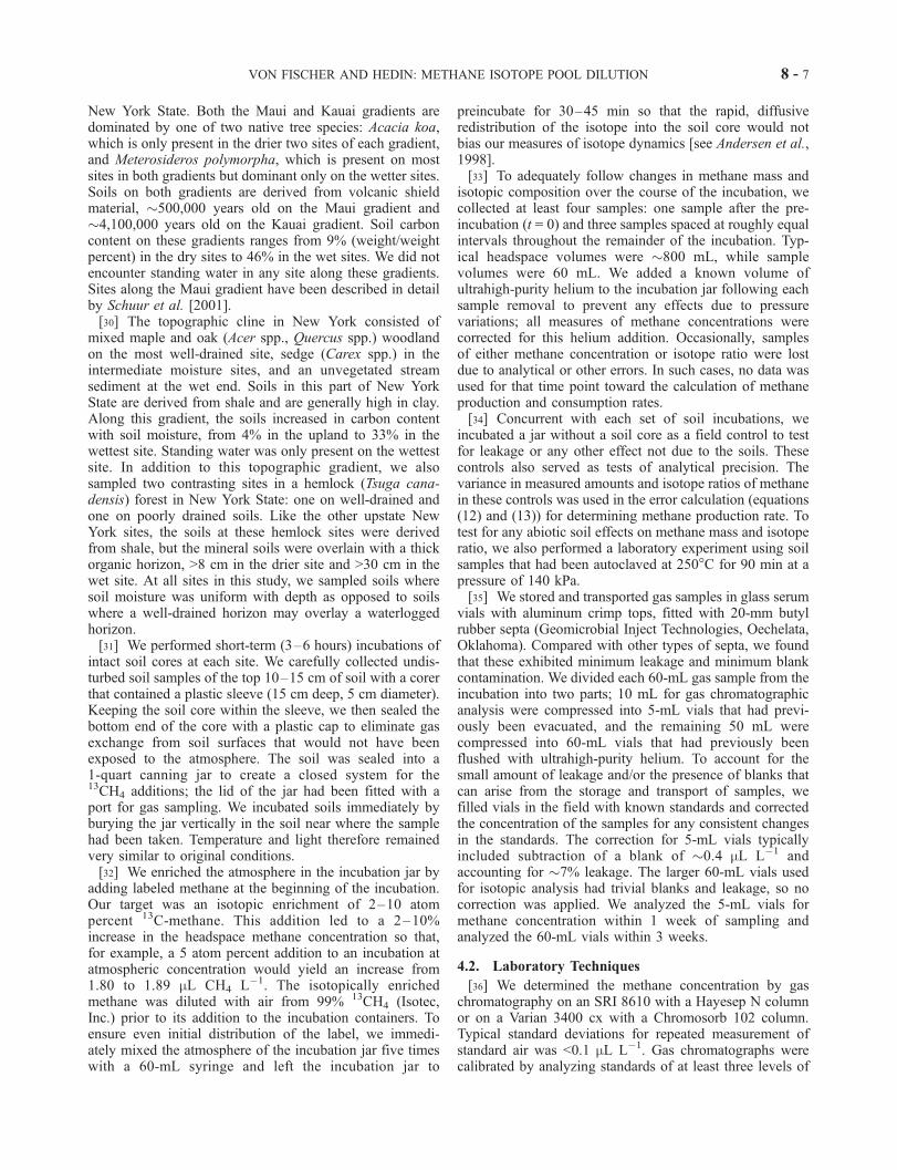
the changes in the amount of labeled methane over time(Figures 4a and 4b) and the changes in the amount andisotope ratio of methane (Figures 4c and 4d) for two soilincubations: one with negative net flux (gross consumption> gross production) and one with positive flux (grossproduction > gross consumption). For the soil with netnegative flux (net consumption of 5.2 mg CH4-C m�2

day�1), we determine k from the data in Figure 4a andcalculate a gross consumption rate of 5.4 mg CH4-C m�2

day�1. The existence of methane production is demonstratedqualitatively by a decline in the methane isotope ratio overthe course of sampling (Figure 4c). We fit equation (11) tothis isotope decline and fit equation (5) to the data for theamount of methane (r2 = 0.99 for fit of equation (11) toisotope data, 0.99 for fit of equation (15) to amount data) andcalculate a gross production rate of 0.18 mg CH4-C m�2

day�1. This incubation illustrated that both productive andconsumptive processes co-occurred in this soil, even thoughtraditional measures of atmosphere-soil methane flux indi-cated net consumption.[42] In contrast, we show in Figures 4b and 4d a soil that

displayed positive methane flux (i.e., net production, 25.4mg CH4-C m�2 day�1). In this case, the fit for the amountof labeled methane versus time (Figure 4b) leads to a grossconsumption rate of 1.1 mg CH4-C m�2 day�1. Our modelfit to the plot of the amount of methane and its isotope ratio(Figure 4d; r2 = 0.98 for fit of equation (5) to amount data,r2 = 0.99 for fit of equation (11) to isotope data) reveal agross methane production rate of 26.5 mg CH4-C m�2

day�1. In this case, the gross methane consumption ratewas considerably less than the gross methane productionrate, despite the elevated abundance of methane resultingfrom methane production.[43] We used empty incubation containers and sterilized

soils to determine if trends in the amount of methane andits isotopic composition can occur in the absence of livesoils and to establish a method detection limit. Our testsshowed that statistically significant rates of methane pro-


duction and consumption only occurred in the presence oflive soil (test for production and consumption >0: p <0.001 in live soil treatment, p > 0.22 for autoclaved soiland no soil treatments, n = 4 for each treatment). Similarly,empty containers that were incubated to serve as controls inthe field displayed rates of methane production and con-sumption not different from zero ( p > 0.9 for bothproduction and consumption). We adopted the averagerates of gross production (0.04 mg CH4-C m�2 day�1)and consumption (0.11 mg CH4-C m�2 day�1) from thefield controls as the minimum detection limit for measure-ment in the field.[44] Our 130 field incubated soils displayed a wide range

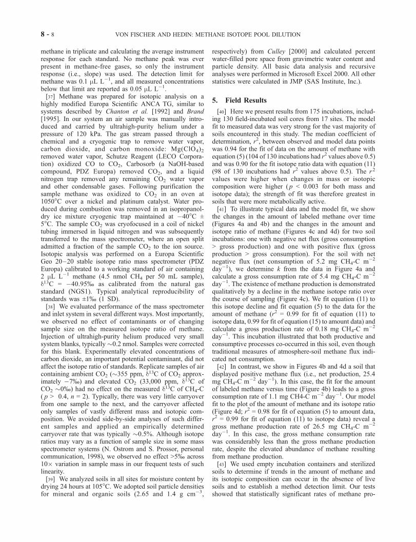
of net methane flux rates, from �8.9 to 926 mg CH4-C m�2

day�1. In Figure 5 we show the contributions of grossmethane production and consumption to the net flux rate,and we partition the range of net fluxes into three catego-ries: those with positive net flux (>0.2 mg CH4-C m�2

day�1), negative net flux (<�0.2 mg CH4-C m�2 day�1),and near zero net flux (between 0.2 and �0.2 mg CH4-Cm�2 day�1). We observed gross rates of methane productionacross more than 4 orders of magnitude (0.04–930 mgCH4-C m�2 day�1), while methane consumption variedacross a much smaller range (0.11–9.2 mg CH4-C m�2

day�1). Occasionally, we measured small, negative produc-tion and consumption rates that are biologically meaning-less but arise from analytical error when rates of the processare very low. These data are included here to illustrate thesituations where they can arise and because elimination ofsuch points can induce bias.[45] Comparisons within net flux categories (i.e., within

columns of Figure 5) provide information about the inter-action between gross production and consumption rates.Soils with negative net flux had only low rates of grossmethane production (<0.5 mg CH4-C m�2 day�1), but ratesof gross methane consumption in these soils ranged from

Figure 4. (a, b) Changes in amount of labeled methane as a function of time and (c, d) changes in totalamount and isotopic composition of methane for field-incubated soils. Symbols mark measured values,while lines are model fits. In Figures 4a and 4b the model fit is for equation (9) to the data, whilein Figures 4c and 4d the model fit is for equations (5) and (11) to the data. Note the log scale on the y axisof Figures 4a and 4b. Arrows identify initial amount of methane and its isotopic composition forincubation. Figures 4a and 4c show measured and model trends for a forest soil from a Hawaiian site withnegative methane flux (P < C ). Figures 4b and 4d show those trends for a soil sample from a wetland sitein New York State with positive methane flux (P > C ).


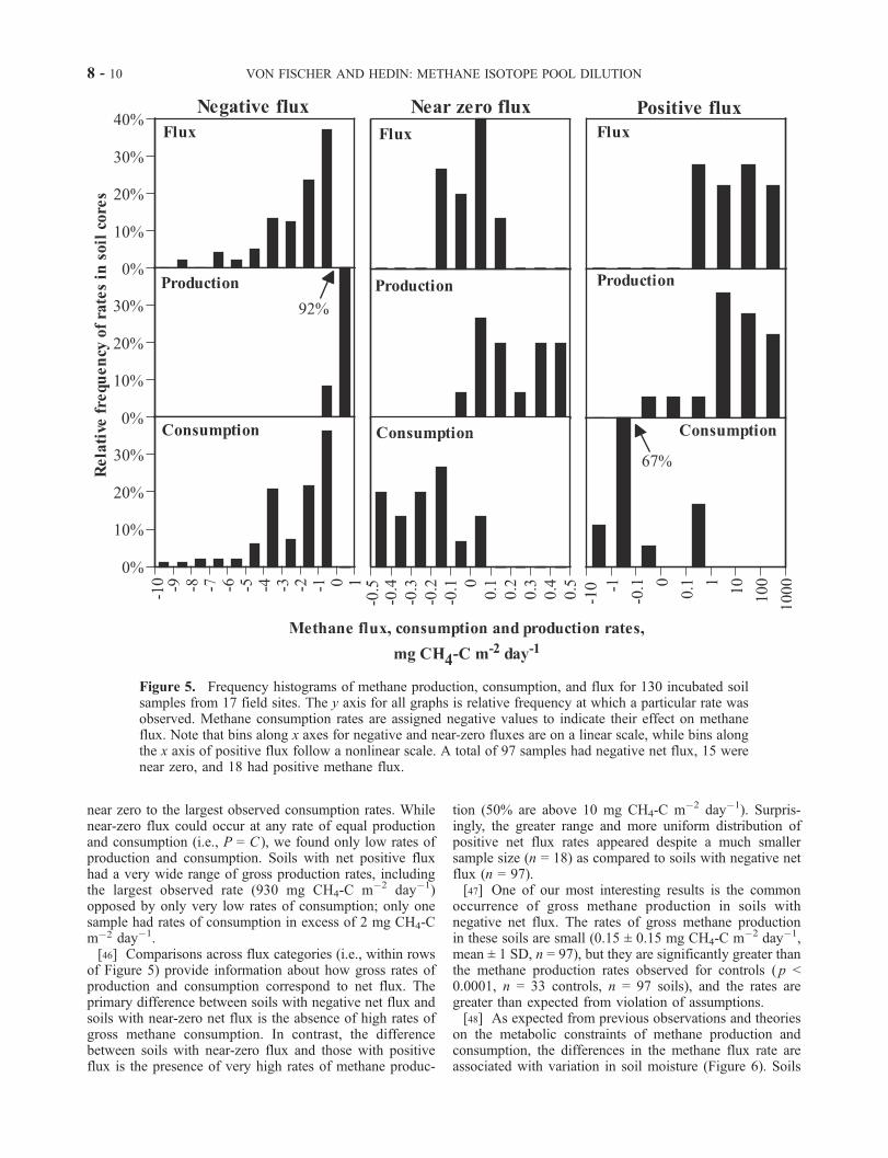
near zero to the largest observed consumption rates. Whilenear-zero flux could occur at any rate of equal productionand consumption (i.e., P = C ), we found only low rates ofproduction and consumption. Soils with net positive fluxhad a very wide range of gross production rates, includingthe largest observed rate (930 mg CH4-C m�2 day�1)opposed by only very low rates of consumption; only onesample had rates of consumption in excess of 2 mg CH4-Cm�2 day�1.[46] Comparisons across flux categories (i.e., within rows

of Figure 5) provide information about how gross rates ofproduction and consumption correspond to net flux. Theprimary difference between soils with negative net flux andsoils with near-zero net flux is the absence of high rates ofgross methane consumption. In contrast, the differencebetween soils with near-zero flux and those with positiveflux is the presence of very high rates of methane produc-

tion (50% are above 10 mg CH4-C m�2 day�1). Surpris-ingly, the greater range and more uniform distribution ofpositive net flux rates appeared despite a much smallersample size (n = 18) as compared to soils with negative netflux (n = 97).[47] One of our most interesting results is the common

occurrence of gross methane production in soils withnegative net flux. The rates of gross methane productionin these soils are small (0.15 ± 0.15 mg CH4-C m�2 day�1,mean ± 1 SD, n = 97), but they are significantly greater thanthe methane production rates observed for controls ( p <0.0001, n = 33 controls, n = 97 soils), and the rates aregreater than expected from violation of assumptions.[48] As expected from previous observations and theories

on the metabolic constraints of methane production andconsumption, the differences in the methane flux rate areassociated with variation in soil moisture (Figure 6). Soils

Figure 5. Frequency histograms of methane production, consumption, and flux for 130 incubated soilsamples from 17 field sites. The y axis for all graphs is relative frequency at which a particular rate wasobserved. Methane consumption rates are assigned negative values to indicate their effect on methaneflux. Note that bins along x axes for negative and near-zero fluxes are on a linear scale, while bins alongthe x axis of positive flux follow a nonlinear scale. A total of 97 samples had negative net flux, 15 werenear zero, and 18 had positive methane flux.


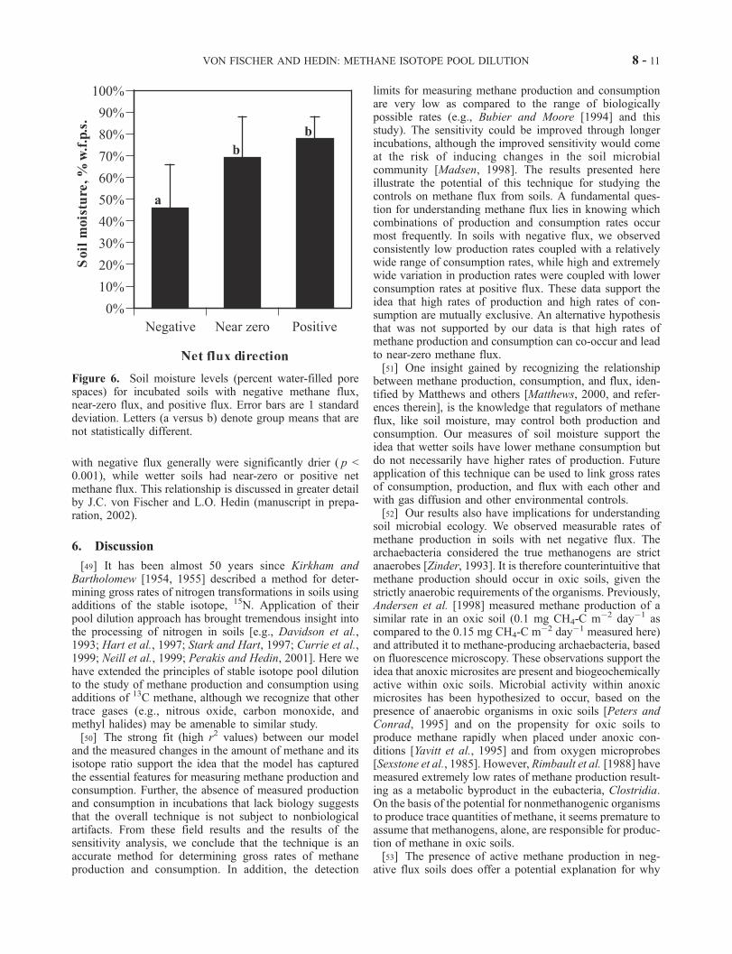
with negative flux generally were significantly drier ( p <0.001), while wetter soils had near-zero or positive netmethane flux. This relationship is discussed in greater detailby J.C. von Fischer and L.O. Hedin (manuscript in prepa-ration, 2002).

6. Discussion

[49] It has been almost 50 years since Kirkham andBartholomew [1954, 1955] described a method for deter-mining gross rates of nitrogen transformations in soils usingadditions of the stable isotope, 15N. Application of theirpool dilution approach has brought tremendous insight intothe processing of nitrogen in soils [e.g., Davidson et al.,1993; Hart et al., 1997; Stark and Hart, 1997; Currie et al.,1999; Neill et al., 1999; Perakis and Hedin, 2001]. Here wehave extended the principles of stable isotope pool dilutionto the study of methane production and consumption usingadditions of 13C methane, although we recognize that othertrace gases (e.g., nitrous oxide, carbon monoxide, andmethyl halides) may be amenable to similar study.[50] The strong fit (high r2 values) between our model

and the measured changes in the amount of methane and itsisotope ratio support the idea that the model has capturedthe essential features for measuring methane production andconsumption. Further, the absence of measured productionand consumption in incubations that lack biology suggeststhat the overall technique is not subject to nonbiologicalartifacts. From these field results and the results of thesensitivity analysis, we conclude that the technique is anaccurate method for determining gross rates of methaneproduction and consumption. In addition, the detection

limits for measuring methane production and consumptionare very low as compared to the range of biologicallypossible rates (e.g., Bubier and Moore [1994] and thisstudy). The sensitivity could be improved through longerincubations, although the improved sensitivity would comeat the risk of inducing changes in the soil microbialcommunity [Madsen, 1998]. The results presented hereillustrate the potential of this technique for studying thecontrols on methane flux from soils. A fundamental ques-tion for understanding methane flux lies in knowing whichcombinations of production and consumption rates occurmost frequently. In soils with negative flux, we observedconsistently low production rates coupled with a relativelywide range of consumption rates, while high and extremelywide variation in production rates were coupled with lowerconsumption rates at positive flux. These data support theidea that high rates of production and high rates of con-sumption are mutually exclusive. An alternative hypothesisthat was not supported by our data is that high rates ofmethane production and consumption can co-occur and leadto near-zero methane flux.[51] One insight gained by recognizing the relationship

between methane production, consumption, and flux, iden-tified by Matthews and others [Matthews, 2000, and refer-ences therein], is the knowledge that regulators of methaneflux, like soil moisture, may control both production andconsumption. Our measures of soil moisture support theidea that wetter soils have lower methane consumption butdo not necessarily have higher rates of production. Futureapplication of this technique can be used to link gross ratesof consumption, production, and flux with each other andwith gas diffusion and other environmental controls.[52] Our results also have implications for understanding

soil microbial ecology. We observed measurable rates ofmethane production in soils with net negative flux. Thearchaebacteria considered the true methanogens are strictanaerobes [Zinder, 1993]. It is therefore counterintuitive thatmethane production should occur in oxic soils, given thestrictly anaerobic requirements of the organisms. Previously,Andersen et al. [1998] measured methane production of asimilar rate in an oxic soil (0.1 mg CH4-C m�2 day�1 ascompared to the 0.15 mg CH4-C m�2 day�1 measured here)and attributed it to methane-producing archaebacteria, basedon fluorescence microscopy. These observations support theidea that anoxic microsites are present and biogeochemicallyactive within oxic soils. Microbial activity within anoxicmicrosites has been hypothesized to occur, based on thepresence of anaerobic organisms in oxic soils [Peters andConrad, 1995] and on the propensity for oxic soils toproduce methane rapidly when placed under anoxic con-ditions [Yavitt et al., 1995] and from oxygen microprobes[Sexstone et al., 1985]. However, Rimbault et al. [1988] havemeasured extremely low rates of methane production result-ing as a metabolic byproduct in the eubacteria, Clostridia.On the basis of the potential for nonmethanogenic organismsto produce trace quantities of methane, it seems premature toassume that methanogens, alone, are responsible for produc-tion of methane in oxic soils.[53] The presence of active methane production in neg-

ative flux soils does offer a potential explanation for why

Figure 6. Soil moisture levels (percent water-filled porespaces) for incubated soils with negative methane flux,near-zero flux, and positive flux. Error bars are 1 standarddeviation. Letters (a versus b) denote group means that arenot statistically different.


incubated soil samples cannot reduce methane concentra-tions to that which is expected based on the enzymaticcapacity of known methanotrophs [Conrad, 1993]. We offerthe testable, alternate hypothesis that methane production,something that we measured commonly in dry soils, wouldcreate a compensation concentration [Conrad, 1994] thatmay be responsible for the apparent threshold. Similarly,hidden methane production may also be responsible for thegenerally lower rates of isotopic fractionation that have beenmeasured for soils as compared to pure cultures of meth-anotrophs [Snover and Quay, 2000]. Perhaps the very lowrates of methane production can provide an importantsource of energy for methane consumers.

Appendix A: Conventions for Reporting IsotopicComposition

[54] The relative abundance of stable isotopes is com-monly reported in one of three notations.1. The first notation gives the ratio of heavy to light

isotopes, R = 13C/12C. This ratio is a ‘‘raw’’ measure madeby isotope ratio mass spectrometers.2. The second notation gives the atom percent of the

heavy isotope, AP = (13C/(12C+13C)100). Atom percentexcess, or APE, expresses the relative abundance of theheavy isotope above natural abundance levels. APE iscalculated as the AP of an isotopically enriched materialminus the AP at natural abundance levels of enrichment.3. The third notation is the delta notation, d13C = ((Rs

� Ra)/Ra)1000, where Rs is the isotope ratio of thesample and Ra is the isotope ratio of a standard. Thisnotation is often used to highlight small differences inisotopic composition that occur near natural abundanceenrichments.

Notation

a fractionation factor for methane consumption.APp atom percent 13C of methane produced in the

soil.APt atom percent 13C of methane at time t.

b concentration of methane in the atmosphere.C, Ct rate of methane consumption.

E sum of normalized error between observed andexpected values.

k first-order constant for methane production.m, mt total amount of methane or the amount at time t.

m0 total amount of methane at t = 0.n, nt amount of labeled methane or the amount at

time t.n0 amount of labeled methane at t = 0.P rate of methane production.

SDobs-AP observed variance in APt over the course of theincubation, in standard deviations.

SDobs-m observed variance in the amount of methaneover the course of the incubation, in standarddeviations.

SDprec-AP precision, or observed variance in APt in fieldcontrols, in standard deviations.

SDprec-m precision, or observed variance in the amount

of methane in field controls, in standard dev-iations.

NAP normalization factor for isotopic compositiondata.

Nm normalization factor for data on the amount ofmethane.

t time.v volume of air in the incubation chamber.

[55] Acknowledgments. This work was supported by grants from theAndrew W. Mellon Foundation, a National Science Foundation ResearchTraining grant graduate fellowship, and a National Aeronautics and SpaceAdministration Earth System Science graduate fellowship. We thank LouDerry, Nathaniel Ostrom, and Todd Walter for their help and advice andthank Jonathan Comstock and Jim Burdett in the Cornell Boyce Thomp-son Stable Isotope Lab for their generous support. We thank PamelaMatson, Ted Schuur, and Peter Vitousek for invaluable comments andassistance with access to field sites. We thank Heraldo Farrington andseveral others for their assistance in the field. Finally, we thank JeffChanton and two anonymous reviewers who provided valuable criticismon this manuscript.

ReferencesAndersen, B. L., G. Bidoglio, A. Leip, and D. Rembges, A new method tostudy simultaneous methane oxidation and methane production in soils,Global Biogeochem. Cycles, 12(4), 587–594, 1998.

Bender, M., and R. Conrad, Kinetics of CH4 oxidation in oxic soils exposedto ambient air or high CH4 mixing ratios, FEMS Microbiol. Ecol., 101,261–270, 1992.

Brand, W. A., Precon: A fully automated interface for the pre-GC concen-tration of trace gases in air for isotopic analysis, Isot. Environ. HealthStud., 31, 277–284, 1995.

Bubier, J. L., and T. R. Moore, An ecological perspective on methane emis-sions from northern wetlands, Trends Ecol. Evol., 9(12), 460–464, 1994.

Chanton, J. P., G. J. Whiting, W. Showers, and P. Crill, Methane flux fromPaltandra virginica: Stable isotope tracing and chamber effects, GlobalBiogeochem. Cycles, 6(1), 15–33, 1992.

Chanton, J. P., G. J. Whiting, N. E. Blair, C. W. Lindau, and P. K. Bollich,Methane emission from rice: Stable isotopes, diurnal variations, and CO2

exchanges, Global Biogeochem. Cycles, 11(1), 15–27, 1997.Cicerone, R. J., and R. S. Oremland, Biogeochemical aspects of atmo-spheric methane, Global Biogeochem. Cycles, 2(4), 299–327, 1988.

Conrad, R., Mechanisms controlling methane emission from wetland ricefields, in The Biogeochemistry of Global Change: Radiative Trace Gases,edited by R .S. Oremland, pp. 317–335, Chapman and Hall, New York,1993.

Conrad, R., Compensation concentration as critical variable for regulatingthe flux of trace gases between soil and atmosphere, Biogeochemistry, 27,155–170, 1994.

Culley, J. L. B., Density and Compressibility, in Soil Sampling and Methodsof Analysis, edited by M. R. Carter, pp. 529–539, CRC Press, BocaRaton, Fla., 2000.

Currie, W. S., K. J. Nadelhoffer, and J. D. Aber, Soil detrital processescontrolling the movement of N-15 tracers to forest vegetation, Ecol.Appl., 9(1), 87–102, 1999.

Davidson, E. A., and J. P. Schimel, Microbial processes of production andconsumption of nitric oxide, nitrous oxide and methane, in BiogenicTrace Gases: Measuring Emissions From Soil and Water, edited byP. A. Matson and R. C. Harriss, pp. 327–357, Blackwell Sci., Malden,Mass., 1995.

Davidson, E. A., P. A. Matson, P. M. Vitousek, R. Riley, K. Dunkin, G.Garciamendez, and J. M. Maass, Processes regulating soil emissions ofNO and N2O in a seasonally dry tropical forest, Ecology, 74(1), 130–139, 1993.

Etheridge, D. M., G. I. Pearman, and P. J. Fraser, Changes in troposphericmethane between 1841 and 1978 from a high accumulation-rate Antarcticice core, Tellus, Ser. B, 44, 282–294, 1992.

Fenchel, T., G. M. King, and T. H. Blackburn, Bacterial Biogeochemistry:The Ecophysiology of Mineral Cycling, 307 pp., Academic, San Diego,Calif., 1998.

Frenzel, P., Methyl fluoride, an inhibitor of methane oxidation and methaneproduction, FEMS Microbiol. Ecol., 21, 25–36, 1996.

Hansen, J. E., M. Sato, A. Lacis, R. Ruedy, I. Tegen, and E. Matthews,


Climate forcings in the Industrial era, Proc. Natl. Acad. Sci., 95, 12,753–12,758, 1998.

Hanson, R. S., and T. E. Hanson, Methanotrophic bacteria, Microbiol. Rev.,60(2), 439–471, 1996.

Harries, J. E., H. E. Brindley, P. J. Sagoo, and R. J. Bantges, Increases ingreenhouse forcing inferred from the outgoing longwave radiation spectraof the Earth in 1970 and 1997, Nature, 410, 355–357, 2001.

Hart, S. C., D. Binkley, and D. A. Perry, Influence of red alder on soilnitrogen transformations in two conifer forests of contrasting productiv-ity, Soil Biol. Biochem., 29(7), 1111–1123, 1997.

Hoefs, J., Stable Isotope Geochemistry, 220 pp., Springer-Verlag, NewYork, 1997.

Houghton, J. T., L. G. Meira Filho, B. A. Callander, N. Harris, A. Katten-berg, and K. Maskell, Climate Change 1995: The Science of ClimateChange, Cambridge Univ. Press, New York, 1996.

King, G. M., In situ analyses of methane oxidation associated with the rootsand rhizomes of a bur reed, Sparganium eurycarpu m, in a Maine wet-land, Appl. Environ. Microbiol., 62(12), 4548–4555, 1996.

King, G. M., Responses of atmospheric methane consumption by soils toglobal climate change, Global Change Biol., 3, 351–362, 1997.

Kirkham, D., and W. V. Bartholomew, Equations for following nutrienttransformations in soil, utilizing tracer data, Soil Sci. Soc. Am. Proc.,18, 33–34, 1954.

Kirkham, D., and W. V. Bartholomew, Equations for following nutrienttransformations in soil, utilizing tracer data, II, Soil Sci. Soc. Am. Proc.,19, 189–192, 1955.

Lelieveld, J., P. J. Crutzen, and F. J. Dentener, Changing concentration,lifetime and climate forcing of atmospheric methane, Tellus, Ser. B, 50,128–150, 1998.

Liptay, K., J. Chanton, P. Czepiel, and B. Mosher, Use of stable isotopes todetermine methane oxidation in landfill cover soils, J. Geophys. Res.,103(D7), 8243–8250, 1998.

Madsen, E. L., Epistemology of environmental microbiology, Environ. Sci.Technol., 32, 429–439, 1998.

Matthews, E., Wetlands, in Atmospheric Methane, edited by M. A. K.Khalil, Springer-Verlag, New York, 2000.

Matthews, E., and I. Fung, Methane emission from natural wetlands: Globaldistribution, area, and environmental characteristics, Global Biogeochem.Cycles, 1(1), 61–86, 1987.

Moosavi, S. C., and P. M. Crill, CH4 oxidation by tundra wetlands asmeasured by a selective inhibitor technique, J. Geophys. Res.,103(D22), 29,093–29,106, 1998.

Neill, C., M. C. Piccolo, J. M. Melillo, P. A. Steudler, and C. C. Cerri,Nitrogen dynamics in Amazon forest and pasture soils measured by N-15pool dilution, Soil Biol. Biochem., 31(4), 567–572, 1999.

Neter, J., W. Wasserman, and M. H. Kutner, Applied Linear StatisticalModels: Regression, Analysis of Variance and Experimental Designs,1181 pp., Irwin, Burr Ridge, Ill., 1990.

Oremland, R. S., and C. W. Culbertson, Evaluation of methyl fluoride anddimethyl ether as inhibitors of aerobic methane oxidation, Appl. Environ.Microbiol., 58(9), 2983–2992, 1992a.

Oremland, R. S., and C. W. Culbertson, Importance of methane-oxidizingbacteria in the methane budget as revealed by the use of a specificinhibitor, Nature, 356, 421–423, 1992b.

Perakis, S. S., and L. O. Hedin, Fluxes and fates of nitrogen in soil of anunpolluted old-growth temperate forest, southern Chile, Ecology, 82(8),2245–2260, 2001.

Peters, V., and R. Conrad, Methanogenic and other strictly anaerobic bac-teria in desert soil and other oxic soils, Appl. Environ. Microbiol., 61(4),1673–1676, 1995.

Petit, J. R., et al., Climate and atmospheric history of the past 420,000 yearsfrom the Vostok ice core, Antarctica, Nature, 399, 429–436, 1999.

Potter, C. S., An ecosystem simulation model for methane production andemission from wetlands, Global Biogeochem. Cycles, 11(4), 495–506,1997.

Potter, C. S., E. A. Davidson, and L. V. Verchot, Estimation of globalbiogeochemical controls and seasonality in soil methane consumption,Chemosphere, 32(11), 2219–2246, 1996.

Rimbault, A., P. Niel, H. Virelizier, J. C. Darbord, and G. Leluan, L-Methionine, a precursor of trace methane in some proteolytic Clostridia,Appl. Environ. Microbiol., 54(6), 1581–1586, 1988.

Roslev, P., N. Iversen, and K. Henriksen, Oxidation and assimilation ofatmospheric methane by soil methane oxidizers, Appl. Environ. Micro-biol., 63(3), 874–880, 1997.

Saarnio, S., J. Alm, J. Silvola, A. Lohila, H. Nykanen, and P. J. Martikai-nen, Seasonal variation in CH4 emissions and production and oxidationpotentials at microsites on an oligotrophic pine fen, Oecologia, 110,414–422, 1997.

Schuur, E. A. G., O. A. Chadwick, and P. A. Matson, Carbon cycling andsoil carbon storage in mesic to wet Hawaiian montane forests, Ecology,82, 3182–3196, 2001.

Sexstone, A. J., N. P. Revsbech, T. B. Parkin, and J. M. Tiedje, Directmeasurement of oxygen profiles and denitrification rates in soil aggre-gates, Soil Sci. Soc. Am. J., 49, 645–651, 1985.

Snover, A. K., and P. D. Quay, Hydrogen and carbon kinetic isotope effectsduring soil uptake of atmospheric methane, Global Biogeochem. Cycles,14(1), 25–39, 2000.

Stark, J. M., and S. C. Hart, High rates of nitrification and nitrate turnoverin undisturbed coniferous forests, Nature, 385, 61–64, 1997.

Sugimoto, A., T. Inoue, N. Kirtibutr, and T. Abe, Methane oxidation bytermite mounds estimated by the carbon isotopic composition of methane,Global Biogeochem. Cycles, 12(4), 595–605, 1998.

Sundh, I., M. Nilsson, G. Granberg, and G. H. Svenson, Depth distributionof microbial production and oxidation of methane in northern borealpeatlands, Microbial Ecol., 27, 253–265, 1994.

Walter, B. P., and M. Heimann, A process-based, climate sensitive model toderive methane emissions from natural wetlands: Application to five wet-land sites, sensitivity to model parameters, and climate, Global Biogeo-chem. Cycles, 14(3), 745–765, 2000.

Wang, W. C., Y. L. Yung, A. A. Lacis, T. Mo, and J. E. Hanson, Green-house effects due to man-made perturbations of trace gases, Science,194(4266), 685–690, 1976.

Whalen, S. C., W. S. Reeburgh, and V. A. Barber, Oxidation of methane inboreal forest soils: A comparison of 7 measures, Biogeochemistry, 16,181–211, 1992.

Whiticar, M. J., Stable isotopes and global budgets, in AtmosphericMethane: Sources, Sinks, and Role in Global Change, edited by M. A.K. Kahlil, pp. 138–167, Springer-Verlag, New York, 1993.

Wieder, R. K., and J. B. Yavitt, Peatlands and global climate change: In-sights from comparative studies of sites situated along a latitudinal gra-dient, Wetlands, 14(3), 229–238, 1994.

Yavitt, J. B., D. M. Downey, G. E. Lang, and A. J. Sexstone, Methaneconsumption in two temperate forest soils, Biogeochemistry, 9, 39–52,1990.

Yavitt, J. B., T. J. Fahey, and J. A. Simmons, Methane and carbon dioxidedynamics in a northern hardwood ecosystem, Soil Sci. Soc. Am. J., 59,796–804, 1995.

Zinder, S. H., Physiological ecology of methanogens, in Methanogens:Ecology, Physiology, Biochemistry and Genetics, edited by J. G. Ferry,pp. 128–206, Chapman and Hall, New York, 1993.

��L. O. Hedin, Department of Ecology and Evolutionary Biology and

Princeton Environmental Institute, Princeton University, Princeton, NJ08544, USA. ([email protected])J. C. von Fischer, Department of Geosciences, Guyot Hall, Princeton

University, Princeton, NJ 08544, USA. ( [email protected])


Separating methane production and consumption with … · Separating methane production and...

Documents

Transcript of Separating methane production and consumption with … · Separating methane production and...