SENTIMENT LEXICON GENERATION WITH CONTINUOUS … · sentiment lexicon generation with continuous...

SENTIMENT LEXICON GENERATION WITH CONTINUOUS

POLARITIES FOR PORTUGUESE USING LOGISTIC

REGRESSIONS AND SEMANTIC MODIFIERS

Renan Araujo Lage

Projeto de Graduacao apresentado ao Curso

de Engenharia de Computacao e Informacao

da Escola Politecnica, Universidade Federal

do Rio de Janeiro, como parte dos requisitos

necessarios a obtencao do tıtulo de Engen-

heiro.

Orientador: Daniel Ratton Figueiredo

Rio de Janeiro

Setembro de 2016

SENTIMENT LEXICON GENERATION WITH CONTINUOUS

POLARITIES FOR PORTUGUESE USING LOGISTIC

REGRESSIONS AND SEMANTIC MODIFIERS

Renan Araujo Lage

PROJETO DE GRADUACAO SUBMETIDO AO CORPO DOCENTE DO CURSO

DE ENGENHARIA DE COMPUTACAO E INFORMACAO DA ESCOLA POLITECNICA

DA UNIVERSIDADE FEDERAL DO RIO DE JANEIRO COMO PARTE DOS

REQUISITOS NECESSARIOS PARA A OBTENCAO DO GRAU DE ENGEN-

HEIRO DE COMPUTACAO E INFORMACAO

Autor:

Renan Araujo Lage

Orientador:

Prof. Daniel Ratton Figueiredo, Ph. D.

Coorientador:

Pedro Henrique Pamplona Savarese, M.S.

Examinador:

Prof. Toacy Cavalcante de Oliveira, DSc.

Examinador:

Bruno Adam Osiek, DSc.

Rio de Janeiro

Setembro de 2016

ii

UNIVERSIDADE FEDERAL DO RIO DE JANEIRO

Escola Politecnica - Departamento de Eletronica e de Computacao

Centro de Tecnologia, bloco H, sala H-217, Cidade Universitaria

Rio de Janeiro - RJ CEP 21949-900

Este exemplar e de propriedade da Universidade Federal do Rio de Janeiro, que

podera incluı-lo em base de dados, armazenar em computador, microfilmar ou adotar

qualquer forma de arquivamento.

E permitida a mencao, reproducao parcial ou integral e a transmissao entre bib-

liotecas deste trabalho, sem modificacao de seu texto, em qualquer meio que esteja

ou venha a ser fixado, para pesquisa academica, comentarios e citacoes, desde que

sem finalidade comercial e que seja feita a referencia bibliografica completa.

Os conceitos expressos neste trabalho sao de responsabilidade do(s) autor(es).

iii

ACKNOWLEDGEMENT

I thank my parents that encouraged me along all my university years. I thank

my girlfriend that supported me while I was immersed in the doing of this work.

I thank my dear friend Pedro and my adviser Daniel that guided me through the

process of making this work. At last, I thank my friends for being who they are and

supporting me in everything.

iv

ABSTRACT

Research in sentiment analysis has hugely increased due to the advent of social

medias and businesses interest on public opinion. Extracting opinion from text

without the need of labeled data makes unsupervised approaches more appealing.

However, many require a sentiment lexicon, a dictionary associating words to sen-

timents with a costly built process. This project proposes an automated approach

to build a sentiment lexicon for the Portuguese language. The method is based on

a supervised learning task that trains a logistic regression model on top of textual

data classified as positive or negative and then extract terms that contribute the

most to the model’s sentiment attribution. These terms are used to build the sen-

timent lexicon with polarities in a continuous range. The use of semantic rules as a

preprocessing step is used to improve the model and subsequent lexicon generation.

Key-words: sentiment analysis, opinion mining, lexicon, logistic regression.

v

Contents

1 Introduction 1

1.1 Sentiment Analysis . . . . . . . . . . . . . . . . . . . . . . . . . . . . 1

1.2 Extracting sentiment from text . . . . . . . . . . . . . . . . . . . . . 2

1.3 Sentiment Lexicon generation . . . . . . . . . . . . . . . . . . . . . . 3

1.4 Objective . . . . . . . . . . . . . . . . . . . . . . . . . . . . . . . . . 4

1.5 Methodology . . . . . . . . . . . . . . . . . . . . . . . . . . . . . . . 5

2 Related Work 6

2.1 Document Sentiment Classification . . . . . . . . . . . . . . . . . . . 6

2.2 Supervised Learning Methods . . . . . . . . . . . . . . . . . . . . . . 7

2.3 Unsupervised Methods . . . . . . . . . . . . . . . . . . . . . . . . . . 8

2.4 Lexicon-based methods . . . . . . . . . . . . . . . . . . . . . . . . . . 8

2.5 Lexicon Generation . . . . . . . . . . . . . . . . . . . . . . . . . . . . 9

2.5.1 Dictionary-based methods . . . . . . . . . . . . . . . . . . . . 9

2.5.2 Corpus-based methods . . . . . . . . . . . . . . . . . . . . . . 10

3 Method Design and Implementation 12

3.1 Logistic Regression . . . . . . . . . . . . . . . . . . . . . . . . . . . . 12

3.1.1 Linear regression . . . . . . . . . . . . . . . . . . . . . . . . . 13

3.1.2 Logistic regression model . . . . . . . . . . . . . . . . . . . . . 14

3.1.3 Bag-of-Words . . . . . . . . . . . . . . . . . . . . . . . . . . . 16

3.1.4 Lexicon extraction . . . . . . . . . . . . . . . . . . . . . . . . 18

3.1.5 Threshold . . . . . . . . . . . . . . . . . . . . . . . . . . . . . 19

3.2 SO-CAL - Semantic Orientation CALculator . . . . . . . . . . . . . . 19

3.2.1 Intensifiers . . . . . . . . . . . . . . . . . . . . . . . . . . . . . 20

vi

3.2.2 Negators . . . . . . . . . . . . . . . . . . . . . . . . . . . . . . 21

3.2.3 Irrealis . . . . . . . . . . . . . . . . . . . . . . . . . . . . . . . 22

3.2.4 Positive bias normalization . . . . . . . . . . . . . . . . . . . . 22

3.2.5 Final score aggregation . . . . . . . . . . . . . . . . . . . . . . 23

3.3 Applying SO-CAL valence shifters to features . . . . . . . . . . . . . 24

4 Lexicon Evaluation 26

4.1 Datasets . . . . . . . . . . . . . . . . . . . . . . . . . . . . . . . . . . 27

4.1.1 Book reviews . . . . . . . . . . . . . . . . . . . . . . . . . . . 28

4.1.2 Hotel reviews . . . . . . . . . . . . . . . . . . . . . . . . . . . 29

4.2 Logistic Regression model hyperparameters . . . . . . . . . . . . . . . 30

4.2.1 SO-CAL valence shifters . . . . . . . . . . . . . . . . . . . . . 30

4.2.2 Valence shifters maximum number of steps . . . . . . . . . . . 30

4.2.3 Class weights . . . . . . . . . . . . . . . . . . . . . . . . . . . 30

4.2.4 Stop Words . . . . . . . . . . . . . . . . . . . . . . . . . . . . 31

4.3 Lexicon extraction parameters . . . . . . . . . . . . . . . . . . . . . . 32

4.3.1 Threshold . . . . . . . . . . . . . . . . . . . . . . . . . . . . . 32

4.3.2 Polarity score conversion . . . . . . . . . . . . . . . . . . . . . 32

4.4 SO-CAL parameters . . . . . . . . . . . . . . . . . . . . . . . . . . . 32


4.5 Word stemming . . . . . . . . . . . . . . . . . . . . . . . . . . . . . . 32

4.6 Performance measurement . . . . . . . . . . . . . . . . . . . . . . . . 33

4.7 Train, validation and test . . . . . . . . . . . . . . . . . . . . . . . . . 35

4.7.1 Same domain test . . . . . . . . . . . . . . . . . . . . . . . . . 35

4.7.2 Other domain test . . . . . . . . . . . . . . . . . . . . . . . . 36

5 Results 38

5.1 Logistic Regression model hyperparameters . . . . . . . . . . . . . . . 38

5.1.1 SO-CAL valence shifters . . . . . . . . . . . . . . . . . . . . . 38

5.1.2 Valence shifters maximum number of steps . . . . . . . . . . . 39

5.1.3 Class weights . . . . . . . . . . . . . . . . . . . . . . . . . . . 39

5.1.4 Stop Words . . . . . . . . . . . . . . . . . . . . . . . . . . . . 39

5.2 Lexicon extraction parameters . . . . . . . . . . . . . . . . . . . . . . 41

vii

5.2.1 Threshold . . . . . . . . . . . . . . . . . . . . . . . . . . . . . 41

5.2.2 Polarity score conversion . . . . . . . . . . . . . . . . . . . . . 42

5.3 Word stemming . . . . . . . . . . . . . . . . . . . . . . . . . . . . . . 42

5.4 SO-CAL parameters . . . . . . . . . . . . . . . . . . . . . . . . . . . 43


5.5 Optimal hyperparameters combination . . . . . . . . . . . . . . . . . 43

5.6 Comparison against other sentiment lexicons . . . . . . . . . . . . . . 44

6 Conclusion 48

6.1 Future Work . . . . . . . . . . . . . . . . . . . . . . . . . . . . . . . . 49

Bibliography 50

viii

List of Figures

3.1 Linear regression line fitted to data points in a scatter plot [1]. . . . . 13

3.2 Logistic sigmoid function fitted to data in scatter plot [2]. . . . . . . . 15

ix

List of Tables

4.1 Book reviews dataset statistics. . . . . . . . . . . . . . . . . . . . . . 28

4.2 Hotel reviews dataset statistics. . . . . . . . . . . . . . . . . . . . . . 29

4.3 Book reviews training dataset sentiment distribution. . . . . . . . . . 36

4.4 Book reviews test dataset sentiment distribution. . . . . . . . . . . . 36

5.1 Highest MCCs obtained for each different test. . . . . . . . . . . . . . 39

5.2 MCC for different maximum number of steps in both datasets with

stemmed words. . . . . . . . . . . . . . . . . . . . . . . . . . . . . . . 40

5.3 Highest MCCs for balanced class weights in cost functions. . . . . . . 40

5.4 Highest MCCs for stop words removal option in different datasets. . . 40

5.5 MCC values for different thresholds in both datasets. . . . . . . . . . 41

5.6 Highest MCCs for binary and raw polarity score conversion options

in both datasets. . . . . . . . . . . . . . . . . . . . . . . . . . . . . . 42

5.7 Highest MCC results on different datasets for stemming words option. 42

5.8 Highest MCC results on different datasets for positive bias normal-

ization option. . . . . . . . . . . . . . . . . . . . . . . . . . . . . . . . 43

5.9 Optimized combination of hyperparameters for each dataset along

with MMC and accuracy. . . . . . . . . . . . . . . . . . . . . . . . . . 44

5.10 Number of positive and negative terms in each sentiment lexicon. . . 46

5.11 Performance and size of each lexicon when tested against the book

reviews test set. . . . . . . . . . . . . . . . . . . . . . . . . . . . . . . 46

5.12 Performance and size of each lexicon when tested against the hotel

reviews dataset. . . . . . . . . . . . . . . . . . . . . . . . . . . . . . . 46

x

Chapter 1

Introduction

1.1 Sentiment Analysis

Opinions are central to almost all human activities since they influence our

behaviors, beliefs and how we see reality. To a considerable degree, we even condition

our choices upon how others evaluate the different possibilities. We seek opinions to

build our own and to assist in taking better decisions. An observation that applies to

individuals as well as to organizations. Businesses and organizations are searching

for the opinion of its consumers or the general public about their products and

services [3].

Opinions and its related concepts such as sentiments, evaluations and emotions are

the subject of study of sentiment analysis or opinion mining. Sentiment analysis

is the task of extracting opinions from text and since early 2000, has grown into one

of the most active research areas in natural language processing [4].

At that time a series of factors started to increase the interest in people’s opinions

and sentiments, leading research in the area to an exponential growth. First, an in-

dustry surrounding sentiment analysis had flourished, providing a strong motivation

for research. Second, from the research and academic perspective, there had been

many challenging problems that have never been studied before. Last, the advent of

social media on the Internet. Blogs, discussion forums, reviews websites and social

networks all flooded the Web with opinionated content available to anyone with a

connection. The presence of social media and its opinionated data intercepts the

1

increasing interest in the sentiment analysis area.

There has always been a necessity to analyse public and consumer opinions. Or-

ganizations conducted opinion polls, surveys and focus groups to gather this data.

Acquiring this kind of information has long been a huge business itself for market-

ing and public relations. Automatically extracting it from, nowadays abundantly

available, public information in the Web is a huge facilitator with a great business

and organizational value.

For these reasons the field has been raising a lot of interest to businesses and so-

ciety in general. Although sentiment analysis has originated from computer science,

it has spread across many areas such as management sciences, economics, social

sciences and even industrial activities, finding its way to be relevant in almost all

domains.

1.2 Extracting sentiment from text

Semantic Orientation (SO) is a measure of opinion or sentiment expressed in text.

It usually captures an evaluative factor (e.g., positive, negative, angry, sad) and an

associated degree that tells how strong this factor is towards a subject topic, person

or idea [5]. Semantic Orientation can be used to analyze public opinion and extract

helpful insights for marketing and business perspectives, such as measures of success

and popularity.

The task of extracting and analyzing semantic orientation from texts has been

seen in the literature with diverging terms: sentiment analysis [6], opinion mining

[6], subjectivity [7][8], analysis of stance [9][10], point of view [11][12], among others.

Within this project scope, the term sentiment analysis is used. Semantic orientation

or polarity refers to the sentiment direction and strength of a text or lexical item.

Polarity score is a numerical value that measures semantic orientation.

The problem of extracting sentiment from text can be categorized in document

sentiment classification, sentence sentiment classification and aspect-based senti-

ment analysis. In document and sentence classification the difference is in the scope

2

of the text unit. On the first we are interested in extracting sentiment from a doc-

ument whereas on the second from a single sentence or clause. Aspect-based sen-

timent analysis is a more complete approach concerned with extracting sentiment

and opinion targets, or entities, related to that sentiment [13].

This project is focused on document level classification and this problem is usually

solved by two main approaches in literature. The supervised classification approach

consists of building classifiers from labeled instances of text that can then be used to

classify novel text [14], essentially a machine learning approach. The lexicon-based

methods are an unsupervised learning approach that uses a sentiment dictionary.

These methods work on the assumption that the overall sentiment of a document

can be derived from individual words or phrases sentiment orientation [15]. In this

project we are mainly interested in the second method, where document sentiment

orientation is obtained from a lexicon. In particular we are interested in how to

build these dictionaries of word’s sentiment, or sentiment lexicons.

1.3 Sentiment Lexicon generation

The lexicon-based approach assumes there is a set of words with prior polarity,

these words have been called opinion words,polar words and sentiment words in

research literature [3]. Positive sentiment words are used to express some desired

states or qualities while negative sentiment words express undesired states or qual-

ities. A sentiment lexicon is a collection of sentiment words, phrases or terms with

their associated semantic orientations and strengths [16]. In a sentiment lexicon

each positive term is usually assigned a positive polarity score, and each negative

expression a negative one.

A lexicon has to be somehow compiled. This can be done in a manual process in

which each word is analyzed by a person, assigned a polarity and included. However,

that would be a laborious task for a large sized lexicon. Many automated approaches

for lexicon generation have been presented in the literature so far. They can be

used, if not by themselves, to bootstrap a lexicon that can be improved latter with

a reduced amount of manual labour.

3

1.4 Objective

The goal of this project is to propose an automated approach to generate a sen-

timent lexicon for the Portuguese language. The method is based on a supervised

learning task that trains a logistic regression model on top of textual data clas-

sified as positive or negative and then extract terms that contribute the most to

the model’s sentiment classification. These terms are then used to build the senti-

ment lexicon along with their polarities score in a continuous range. This approach

yields a domain specific, or context-aware, lexicon. Which means each word’s as-

sociated sentiment is specific to a single theme, formality, format and/or structure

present in the corpus used. Since many words’ semantic orientation are specific to a

context[17], when the generated lexicon is used by lexicon-based methods in a cor-

pus of the same domain it was built on, the method should correctly classify novel

data with a higher accuracy than with general-purpose lexicons.

In order to attain our main objective we also design and implement a Por-

tuguese version of the SO-CAL (Semantic Orientation CALculator), a lexicon-

based method for sentiment analysis used to evaluate the generated lexicon. The

method uses semantic rules that affect words’ semantic orientation to improve its

prediction when compared to a general lexicon-based method that just aggregates

words’ polarities with no previous treatment.

Finally, the semantic rules designed for SO-CAL will also be used as a prepro-

cessing step for the logistic regression model features (words and terms). By taking

into account words semantic context, the generated lexicon should have an improved

quality over one that doesn’t.

The trained logistic regression model could also be used as a sentiment classifier.

However, the approach of generating a lexicon from it presents at least two advan-

tages over using the model itself. First it generates a sentiment lexicon that can

be used by a number of other more sophisticated lexicon-based algorithms, such as

SO-CAL itself. Second, by controlling in what degree a term is accepted as part

of the sentiment lexicon, we can build a more general and less fitted lexicon that

performs well even on data unrelated to data it was built on.

4

1.5 Methodology

In order to evaluate and test our hypothesis a pipeline of tasks needs to be built.

Those tasks are further explained in Chapters 3 and 4 and can be briefly presented

as:

• Train a logistic regression model on top of a labeled dataset of polarized texts.

• Select terms whose logistic regression estimated coefficients indicates a signif-

icant contribution towards a sentiment.

• Build a lexicon with those terms in which polarity scores are derived from the

logistic regression coefficients.

• Apply the SO-CAL method to a dataset using the generated lexicon.

• Measure how well the method correctly classified sentiment.

Each of those tasks has a number of hyperparameters and options that can affect

the final result. The impact of each of these options on the quality of the gener-

ated lexicon is analysed. Also, the performance of the SO-CAL method using the

generated lexicon is compared to using other publicly available lexicons, with two

different datasets.

Chapter 2 presents related works in the area of automatic lexicon generation and

sentiment analysis, focusing mainly in unsupervised approaches. Chapter 3 the

theoretical background and methodology used along this project is presented. The

evaluation process along with hyperparameters and other options are detailed in

chapter 4. Chapter 5 exhibits results and analyse them. The last chapter shows a

conclusion of the work done in this project and incites future work.

5

Chapter 2

Related Work

The sentiment analysis research field is large and rapidly growing. There is a great

amount of work dedicated to this subject and its related concepts. Since our interest

relies on automatic lexicon generation and document sentiment classification using

lexicon-based methods, this chapter focus on exposing research done in these fields,

only grasping on other subjects like supervised learning methods.

2.1 Document Sentiment Classification

Document sentiment classification is perhaps the most extensively studied

topic in sentiment analysis [6]. The task considers the whole document as a target

to be classified as expressing a positive or negative opinion or sentiment.

Document sentiment classification assumes that the opinionated document ex-

presses opinion on a single entity and contains opinions from a single author. This

assumption fits reviews of products and services well. They are usually an evalua-

tion of a single subject written by a single person. However, it may not hold true

for blog posts, forum discussions and other more complex text pieces.

Techniques for document classification are divided into two categories: the super-

vised learning methods and unsupervised methods. A general view of supervised

learning methods is in the next section and unsupervised methods are presented

later.

6

2.2 Supervised Learning Methods

Sentiment classification is usually approached in literature as a classification prob-

lem with two classes, positive and negative[3]. Most research papers disregard the

neutral class, facilitating the task, but it is possible to use it.

Being a text classification problem, any supervised learning method can be used.

Naıve Bayes and support vector machines (SVM) are commonly used to solve this

problem [18][19]. Perhaps the first paper to publish a supervised learning method

in sentiment analsis was the one by Pang, Lee and Vaithyanathan [14]. They clas-

sified movie reviews into positive and negative classes. The authors concluded that

both Naıve Bayes and SVM performed quite well using bag-of-words (or unigram)

features, although a number of other feature options were tried.

Like in most machine learning applications, an effective selection of features can

be key to improve accuracy. Research has been done experimenting with a large

number of features for sentiment classification, such as:

Terms and their frequency. The most common features are individual words

or unigrams associated with their frequency count. These frequencies can also be

weighted by inverse document frequency, namely the tf-idf scheme from information

retrieval. These features are highly effective for sentiment classification as well as

traditional text classification.

Part of speech. The use of part-of-speech (POS) as a feature may treat dif-

ferently words with distinct POS tags. Since adjectives are describing words that

mainly qualify nouns, sentiment is mostly associated to adjectives. Differentiating

features by their part-of-speech can be beneficial to the model.

Sentiment shifters. Sentiment shifters are expressions that can change the

semantic orientation of neighboring words, e.g., from positive to negative. They will

be better explained in Chapter 3.

7

2.3 Unsupervised Methods

Perhaps the first unsupervised method for sentiment analysis was the one intro-

duced by Turney [15]. It performs sentiment classification based on a set of fixed

syntactic patterns that are likely used to express opinions. These patterns are based

on POS tags and are used to identify opinions in text. Then to identify semantic

orientation a measure was defined: the pointwise mutual information (PMI). PMI

is a measure of the statistical dependence degree between two terms. The sentiment

orientation (SO) was then calculated by the formula:

SO(phrase) = PMI(phrase, "excellent") - PMI(phrase, "poor")

The method doesn’t need a lexicon as it only requires two words with previously

known semantic orientation, excellent and poor. Its classification accuracies varied

from 84% in automobile reviews to 66% in movie reviews.

Feng et al. [20] compared PMI to three other measures of association using differ-

ent corpora. Those measures are Jaccard, Dice, and Normalized Google Distance.

The method was applied on top of data from Google indexed pages, Google Web IT

5-grams, Wikipedia, and Twitter. Their work concluded that PMI perfomed better

when used on the Twitter corpus.

2.4 Lexicon-based methods

Lexicon-based methods are a type of unsupervised classification approach

whose key characteristic is the use of a dictionary of sentiment terms and their

polarities, a sentiment lexicon. This approach was first used by Hu and Liu [13] in

aspect-based sentiment analysis. Kim and Hovy [21] also used it for sentence-level

sentiment classification.

A general lexicon-based method sums up the polarity scores of all sentiment terms

in the document. The document’s semantic orientation is classified as positive if the

sum is positive, negative if the sum is negative, and neutral if the sum is 0. However,

many approaches expand on that base method in a number of ways.

8

The incorporation of intensification and negation can refine the method when

calculating a document’s sentiment [22][23][16]. Polanyi and Zaenen [24] showed

there are other factors that can affect the sentiment orientation of a particular

term. These factors are called valence shifters (or sentiment shifters) and are

further explained in Chapter 3.

Taboada et al. [16] implemented and extended this ideas further by considering

finer cases and selecting better values for valence shifters modifiers. This method

is named SO-CAL (Sentiment Orientation CALculator) and it is implemented and

adapted to the Portuguese language in this project.

2.5 Lexicon Generation

There are three main approaches to compile sentiment terms: manual ap-

proach, dictionary-based approach and corpus-based approach. It was already stated

that the manual approach is laborious and time-consuming, this favors an automatic

approach to the problem.

2.5.1 Dictionary-based methods

Using a dictionary to compile sentiment words is an obvious approach because

most dictionaries list synonyms and antonyms for each word, e.g., WordNet [25].

Therefore, a simple method is to choose a few seed sentiment words to bootstrap

based on the synonym and antonym structure of a dictionary [13][26]. A manual

inspection step can be undertaken after creation to fix any errors.

There are a number of dictionary-based methods that use graphs in the genera-

tion process. Blair-Goldensohn et al. [27] presented a bootstrapping method that

uses a positive seed set, a negative seed set and a neutral seed set. The approach

works based on a directed, weighted semantic graph in which neighboring nodes are

synonyms or antonyms of words from WordNet and are not part of the seed neutral

set. The neutral set is used to stop the propagation of sentiment through neutral

words. Each word sentiment score is attributed through iterations of a modified

9

version of the label propagation algorithm [28]. The final scores are used as polarity

values for each word.

Rao and Ravichandran [29] compared three graph-based semi-supervised learning

methods that separate positive and negative words given a positive seed set, a neg-

ative seed set, and a synonym graph extracted from WordNet. Label propagation

had a significantly higher precision and low recall in comparison.

Esuli and Sebastiani [30] used supervised learning to classify words into positive

and negative classes. A set P of positive seed words and a set N of negative seed

words is initially given, the two seed sets are first expanded using synonyms and

antonyms from a dictionary to generate the expanded sets P’ and N’. Then the

algorithm uses all the glosses in the dictionary for each word in P ′ ∪N ′ to generate

a feature vector. A binary classifier can then be trained on top of those features.

Esuli and Sebastiani [31] implemented an improved version of these classifiers using

different algorithms and built the SentiWordNet, a sentiment lexicon for every term

in the WordNet dictionary.

2.5.2 Corpus-based methods

The corpus-based approach has been used in two main scenarios:

1. Given a seed list of known sentiment words, discover other sentiment words

and their semantic orientations from a domain corpus [32][13][33].

2. Use a domain corpus to adapt a general-purpose sentiment lexicon to a specific

domain [34][35].

Although the corpus-based approach may also be used to build a general-purpose

sentiment lexicon, by using a very large and diverse corpus, the dictionary-based

approach is usually more effective because a dictionary contains all words[3]. Corpus-

based methods should be used if there is an interest in working with domain specific

sentiment lexicons.

10

This project’s method of building a lexicon can be categorized as a corpus-based

method since it uses a corpus of data to generate a lexicon. However, it does not

fit in the typical use-case of this type of approach. It works through a supervised

learning method instead since it trains a logistic regression model on top of the

corpus and extract the sentiment lexicon from it. The next chapters will explain

this process in details.

11

Chapter 3

Method Design and

Implementation

In order to understand the process of generating a lexicon from a logistic regression

model, logistic regression needs to be minimally understood. Specifically how the

model parameters, or coefficients, are estimated from data. Logistic regression will

be used to train a model on top of a collection of texts classified as positive or

negative. There’s also a need to understand the SO-CAL method for sentiment

analysis since, besides being used to evaluate the generated lexicon, part of the

method will be used as a preprocessing step for the logistic regression features. In

an attempt to improve the overall quality of the lexicon. This chapter will describe

these concepts and how they fit together in the task of generating a sentiment

lexicon.

3.1 Logistic Regression

Logistic regression is a linear model developed by statistician David Cox

in 1958[36]. It can be considered a discrete choice model, in the sense that it

estimates the probability of a binary response based on one or more independent

variables/features. This model fits well as a solver to binary classification problems,

such as the one presented by sentiment analysis.

12

For a better understanding of logistic regression, the linear regression model is

presented first and then we can see how logistic regression derives from it and is in

fact a special case of the generalized linear model [37].

3.1.1 Linear regression

The linear regression function models the relationship between a scalar de-

pendent variable and one or more independent variables/features as a linear func-

tion. The model is used to predict data whose outcome is in the form of continuous

numerical values. Its formula can be defined as:

hθ(x) = θ0 + θ1x1 + ...+ θixi + ...+ θnxn = θTx

In which x i is an input variable/feature, θi is a linear function coefficient estimated

from the collection of examples in the training data, n is the the total number of

features and the last equation is a vectorized form of the previous equation.

A linear regression model estimates parameters for a linear function that better

fit the training data. The plot in Figure 3.1 is an example of a linear function fitted

to data points in a scatter plot.

Figure 3.1: Linear regression line fitted to data points in a scatter plot [1].

The values of θ can be learned from a collection of example data by minimiz-

ing a specific cost function. This can be done with techniques such as the least

13

squares method where the sum of squared residuals is minimized, a residual being

the difference between an observed value and the fitted value provided by the linear

regression model. The least squares cost function can be written as:

C(θ) =1

2m

m∑i=1

(hθ(x(i))− y(i))2

Where θ are chosen linear coefficient parameters, m is the number of examples in

the dataset, hθ(x(i)) is the value predicted by the model for the set of features x in

example i and y(i) is the real dependent variable value in example i.

Optimized values for the θ coefficients can be obtained by minimizing the cost

function for θ. The sum of squared residuals is a convex function and therefore has

only one minimum. Finding this minimum is a problem with a closed-form solution

that uses matrix calculus to differentiate with respect to θ and set equal to zero.

Thus, making it simple to calculate. With the estimated optimized parameters the

model can predict more accurate values for novel input data.

Linear regression presents itself as an effective way of predicting continuous data

outcomes. However, if the dependent variable is not a continuous numerical value

but is instead a category or label, there are other models that can can better fit the

data and increase accuracy in predictions [38]. The logistic regression model take

the ideas from linear regression and adjust them to binary outcomes.

X(m,n) =

x(n), for 0 ≤ n ≤ 1

x(n− 1), for 0 ≤ n ≤ 1

x(n− 1), for 0 ≤ n ≤ 1

= xy

3.1.2 Logistic regression model

The logistic regression model comes to address the problem of having out-

comes in the form of categories, also known as labels or classes. The outcome of

a single trial is now described as the probability of a given trial to be in a given

category. In simplest form, this means that we’re considering just one outcome

variable and two states of that variable: either 1 or 0, being or not in the category.

14

This probability is modeled using a logistic or sigmoid function. Its formula can be

defined as:

g(z) =1

1 + e−z

In the above formula, g(z) is the logistic function that will predict the outcome and

z is the same linear regression function previously presented. In that way, logistic

regression fits the linear regression function in a model that can predict a binary

outcome. The expanded formula can be written as:

hθ(x) =1

1 + e−θTX

A logistic regression function plot fitted to data can be seen in Figure 3.2. The

horizontal axis is the linear regression function values z, the vertical axis is the

logistic regression function g(z), blue dots represent data in category blue, red dots

data in opposing category red and the green curve a logistic regression function

fitted to this data.

Figure 3.2: Logistic sigmoid function fitted to data in scatter plot [2].

15

Suppose a red category represented by the number 1 and an opposing blue cate-

gory represented by 0. The graph in Figure 3.2 shows that when the z function (the

linear regression function) value is greater than 0.5, the probability that it belongs in

category red is greater than 0.5, resulting in its classification to red. Whereas when

z is less than 0.5 and the probability also less than 0.5, the outcome is classified in

the opposing blue category. In this way, this model can classify the input features

into opposing or binary categories. Logistic regression can be expanded to deal with

multiclass problems as well [39] but that is of no interest since within this project’s

scope the only interest relies on classifying data in two categories: positive (+1) and

negative (-1).

In the same way as linear regression, θ parameters that better fit the data must

be estimated. This can be done in the same manner, by minimizing a cost function.

However, when applying the same method as in linear regression, the sum of squared

residues, the resulting cost function doesn’t have normally distributed residuals.

Which means it’s not possible to find a closed-form expression for the coefficient

values[40].

The minimization of cost function for logistic regression can be solved by a num-

ber of numerical methods such as gradient descent, conjugate gradient, the Broy-

den–Fletcher–Goldfarb–Shanno algorithm (BFGS) and its limited memory version

L-BFGS [41]. However, detailing cost functions and how to minimize them is out of

the scope of this project as the presented knowledge is sufficient to understand how

the model can be used to build a sentiment lexicon. Specifically our interest relies

on the fact that in a logistic regression model, each input feature has an associated

coefficient θi that is learned from the training data. This coefficients represent the

contribution that each feature gives towards the target category and this intuition

will be key to understand how the lexicon is extracted from the model.

3.1.3 Bag-of-Words

So far logistic regression presents itself as a way to classify numerical data

in binary categories. However, data in sentiment analysis is textual. A way to

16

represent text as a numerical feature is required, hence the Bag-of-Words model

[42].

In the Bag-of-Words model, a text (such as a sentence or a document) is rep-

resented as the bag (multiset) of its words, disregarding grammar and even word

order but keeping multiplicity. They are usually used to generate features for text

classification algorithms. The most common type of features extracted from this

model is the term frequency, the number of times a term appears in the text. How-

ever, a number of others features can be extracted from the text. One could want to

normalize the term frequencies in a document by weighting them with the inverse

of document frequency in the entire collection of documents, namely tf-idf [43], or

simply use a binary feature indicating presence or absence of a term in a text.

A Bag-of-Words could be used to represent an individual term, a text or the entire

collection of texts, the whole corpus. An example of an array representation for each

of these categories in a corpus composed of two documents can be seen below:

(1) Mary likes books. She likes comics too.

(2) Peter also likes comics.

The entire dictionary of words that appear in a corpus can be represented by an

array of terms. And the term frequency in a text piece by another array of same

size, whose indices point to the respective term in the first array, and whose values

indicates the term frequency in that text. An array of the whole vocabulary of terms

for our corpus would be:

["Mary", "Peter", "likes", "also", "books", "she", "comics", "too"]

An individual representation of a term in the corpus, Mary in this case:

[1, 0, 0, 0, 0, 0, 0, 0]

The individual words array can be summed to represent an entire document with

its respective words frequencies.

(1) [1, 0, 2, 0, 1, 1, 1, 1]

(2) [0, 1, 1, 1, 0, 0, 1, 0]

17

The entire corpus could be represented by the sum of document arrays, although

that has no use as a feature for text classification:

[1, 1, 3, 1, 1, 1, 2, 1]

With a Bag-of-Words model, features can be generated from text. Making it

possible to train a logistic regression model on top of labeled textual data, in our

case data labeled with positive or negative sentiment.

3.1.4 Lexicon extraction

By using Bag-of-Words, each document in a corpus is represented by a vector

of terms’ frequencies that when labeled as positive or negative can be used as features

to train a logistic regression model.

Logistic regression estimates coefficients that better fit the training data. These

coefficients are associated to each feature in our vector, that is to each term in

our corpus vocabulary. Which means every term in the corpus has an associated

coefficient that represents its individual contribution in the classification process.

Since positive and negative labels are represented by the numbers +1 and -1, terms

that contribute towards a positive classification would have positive values whereas

ones that contribute towards a negative label would be negative.

The lexicon extraction process can be described in two steps:

1. Each term’s coefficient is analyzed and a decision about whether or not that

term will be part of the lexicon has to be made.

2. The coefficient is converted to a polarity score that expresses the intensity

of the sentiment. It can be the coefficient value itself, or a binary indicating

positiveness or negativeness.

A simple way to generate a lexicon would be to split our vocabulary in terms

whose coefficients are positive, and ones whose coefficients are negative. These two

separated groups of terms represent opposing contributions towards the sentiment

18

classification task. A group that contributes towards positive labeling and one to-

wards negative. The lexicon can be built by assigning a positive polarity to terms

with positive coefficients and a negative polarity to terms with negative ones. Terms

are considered neutral and are not included in the lexicon if their coefficient equals

zero.

However, this simple method may not generate the best lexicon as it only marginally

take into account words that are neutral. In order to effectively disregard neutral

words and select in which degree terms are accepted in the lexicon a parameter can

be defined. The threshold parameter will be presented next.

3.1.5 Threshold

Even though all words will have an associated coefficient, not every word has an

intrinsic polarity. The so called neutral words will have near zero contribution in the

task of labeling a document. These words should not be present in the generated

lexicon as they would supposedly produce erroneous classifications and lower the

overall accuracy of the sentiment analysis task. A minimum absolute value for the

coefficients must be defined to separate neutral words from polarized ones. A value

under which words won’t be included as part of the generated lexicon. Within this

project scope this value will be named threshold.

The process of creating a lexicon is refined by using a threshold value. A number

of others parameters can also have a direct influence in the lexicon generation process

and those are presented in the evaluation chapter. The SO-CAL sentiment analysis

algorithm and how it can further improve the lexicon generation is presented next.

3.2 SO-CAL - Semantic Orientation CALculator

SO-CAL is a lexicon based method to extract sentiment from text, therefore

a way to solve the sentiment analysis problem. It follows the work of Osgood, Suci

and Tannenbaum [5] by making two assumptions: individual words have what is

referred to as prior polarity, that is, a semantic orientation independent of domain;

and that said semantic orientation can be expressed as a numerical value. These

19

same assumptions have also been adopted by several lexicon based methods for

sentiment analysis [44][21].

A general lexicon based method for sentiment analysis can be described as: for

all words in a text that are present in the lexicon, retrieve their polarity scores and

aggregate them to reach a single score for the text. SO-CAL starts with this same

idea but expands it in a number of ways. Concepts like limiting the polarity score’s

range, applying multipliers to polarities according to semantic rules, the so called

valence shifters, and taking into account statistical events, such as a higher occur-

rence of positive words in human generated text are all considered and implemented

in the SO-CAL algorithm. The method was first presented by Taboada and Grieve

in 2004 [45] and has gone through a number of improvements in later works [23][16].

This project’s implementation of the SO-CAL method took some of those ideas

and applied them to the Portuguese language. Savarese [46] has also implemented a

similar version of the SO-CAL algorithm for the Portuguese language. This section

will present the method’s steps that were adopted in this project, starting with

valence shifters.

Valence shifters were first presented in the work of Polanyi and Zaenen [24] and

were used and expanded in SO-CAL. They are an attempt to better reflect sentiment

in a text by applying a set of semantic rules that can capture how a word’s sentiment

orientation can be affected by nearby words. Valence shifters can be defined as

lexical items that have the property of modifying other neighboring lexical items

semantic orientation. They can be classified into 3 different categories: intensifiers,

negators and irrealis. Their description and effect on other word’s polarities is

described next.

3.2.1 Intensifiers

Intensifiers themselves can be classified into two major categories: amplifiers

increase the polarity of neighboring lexical items whereas downtoners decrease it

[47]. Examples of amplifiers are: muito (very), mais (more) and bastante (quite).

Whereas pouco (little) and quase (almost) are downtoners.

20

Each intensifying word has a percentage multiplier associated with it and they

affect neighboring words semantic orientation by applying this multiplier to their

polarities.

Besides the multiplier values, an intensifier can affect the neighbouring semantic

orientation in different ways. It can be referring only to the following word, it can

refer to a previous one or it can intensify words that are located far away from the

intensifier. Differentiating between all those distinct situations and applying the

intensifiers accordingly would be an arduous task. This project’s implementation

takes a simpler approach by applying multipliers in both directions until a clause

break is hit or a maximum number of words is affected, being this last parameter

configurable. Examples of clause breakers are punctuation marks and some connec-

tives like mas (but) and portanto (therefore).

An example of how an intensifier can change another word’s polarity, a downtoner

in this case, is in the sentence A sopa quase me agradou. If agradou has a polarity

score of 2 and quase has a -50% modifier, the final polarity score for agradou is 1.

3.2.2 Negators

An obvious approach to negation is to simply reverse the polarity of words

next to a negator. The polarity score of bom (good) in nao e bom (not good) would

change from 3 to -3. This approach is known as switch negation[48].

However a number of problems have been found with this method[16][22][49].

Taboada and Brooke[16] proposed a new method called shift negation in which

the polarity score is shifted towards the opposite polarity by a fixed amount, in

their work this value was fixed to 4. This project uses switch negation because shift

negation with a fixed value of 4 was targeted on their lexicon whose polarities scores

ranged from -5 to 5 and in this project numerous lexicons with varying ranges are

used.

When a negator is found, the negation modifier is applied to the following lexical

items until a clause break is found or the maximum number of affected words is

21

reached.

3.2.3 Irrealis

There are some markers in a sentence that indicates that words in a sentence

may not be reliable for the purposes of sentiment analysis. These markers are

referred to as irrealis and are usually associated with non-factual contexts. In

Portuguese, these markers are mostly revealed by the use of subjunctive mood. But

also include the use of imperative language, conditional markers, questions and some

verbs like espero (expect) and duvido (doubt).

Their presence in a sentence can change the meaning of polarized words in a subtle

and sometimes unclear way. For example:

1. Com aquele elenco, o filme deveria ser bom, mas nao e. (With that cast, the

movie should be good but it isn’t).

2. Apesar de tudo, o filme deveria ser considerado o melhor do ano. (Neverthe-

less, the movie should be considered the best of the year).

In the first sentence, the correct interpretation would be for the word deveria

(should) to revert the sentiment orientation of bom (good), which is an approach

supported by the contrast revealed in the mas (but) clause. However, in the second

sentence deveria should not reverse the positive meaning given by melhores (best).

The confusing nature of this type of markers and the fact that they rarely express

facts, make it better to ignore the semantic orientation of words that are in the

same clause. Therefore, words in the same clause of an irrealis marker loose their

sentiment intensity, reducing their polarity scores to 0.

3.2.4 Positive bias normalization

Kennedy and Inkpen[22] observed that lexicon-based methods generally show

a positive bias, which is probably due to a universal human tendency to favor positive

language[50]. This problem can be overcome by simply shifting the numerical cut-

off point between positive and negative reviews[51]. However, in the latest SO-CAL

22

paper[16], an alternative was adopted: being negative expressions relatively rare,

they are given more cognitive weight and therefore an amplified polarity score when

they do appear. This is done by amplifying the final score of any negative expression

in a fixed amount (50% was used in this project).

This alternative approach has a small advantage on average over the former,

and is more theoretically satisfying. Also, the positive bias normalization step has

positively affected the overall performance in the most significant way across all

other SO-CAL measures[16]. Its analysis will indicate whether the positive bias also

exists in the Portuguese language or is restricted to English.

3.2.5 Final score aggregation

The final polarity score for a text can be aggregated from individual word’s

polarity in a number of ways. In the SO-CAL method the individual polarized words

scores are simply summed, after applying all modifiers to it, and then averaged by the

total number of polarized words in a text. This project has no interest in comparing

degrees or intensities of sentiment in texts, so there is no use in averaging the final

score. In fact, since the only interest relies on the the predicted positive or negative

sentiment for a given text, any numerical value variation can be disregarded. In that

way, scores greater than 0 are labeled as positive and lesser are labeled as negative,

0 or neutral scores are discarded.

An example to illustrate valence shifters and score aggregation in a sentence can

be seen below:

O programa era lento mas muito divertido.

(The program was slow but very funny)

The polarity scores for each word in the sentence are:

["O", "programa", "era", "lento", "mas", "muito", "divertido"]

[0, 0, 0, -1, 0, 0, +1]

23

The word muito (very) is an intensifier of the amplifier kind with a modifier of

+100%. In that way, after applying valence shifters the final score of each word is:

[0, 0, 0, -1, 0, 0, +2]

And the sentence final polarity score is −1 + 2 = 1 and is therefore a sentence

with positive sentiment.

3.3 Applying SO-CAL valence shifters to features

The SO-CAL algorithms takes an interesting approach when dealing with

the semantic context of words through valence shifters. By analysing context and

applying the same method to Bag-of-Words features, these features may more ac-

curately reflect the real contribution of each term in the overall sentiment. This

section details how valence shifters can be applied to and improve Bag-of-Words

features.

First, we need to analyse how not taking into account the semantic context is prej-

udicial to our model for the task of sentiment analysis. Suppose a corpus composed

of these two sentences with associated sentiment:

(1) "Movies are great", positive (+1)

(2) "Movies are not great", negative (-1)

The array of terms and the Bag-of-Words representation accompanied by the

sentiment score for each sentence is:

["Movies", "are", "great", "not"]

(1) [1, 1, 1, 0], +1

(2) [1, 1, 1, 1], -1

When estimating coefficients for the model, the only feature differentiating the

two samples is the word not present in the negative sample. Which means the

model will learn that not is a word that contributes towards a negative sentiment

and therefore has a negative prior polarity and sentiment score. While the other

24

words, present in every sample of the corpus, by not contributing towards any label

will be considered neutral words. However, those are wrong assumptions. The word

not by itself has no negative connotation, it however gives a negative connotation

to another word next to it that usually has a positive one: great.

The same features with valence shifters applied, specifically switch negation,

would yield:

["Movies", "are", "great", "not"]

(1) [1, 1, 1, 0], +1

(2) [1, 1, -1, 1], -1

The model would still learn that not contributes towards the negative sentiment

in this corpus, but it would most importantly learn that great negatively contributes

towards a negative sentiment. Which means it’s considered a positive term.

The fact that semantic context affects how words contribute towards a sentiment

label is true for all presented valence shifters. Therefore, it is possible to improve

our model for sentiment analysis by applying those rules as a preprocessing step for

our features.

25

Chapter 4

Lexicon Evaluation

The hypothesis of a sentiment lexicon generated from a logistic regression model

needs to be evaluated beyond the manual observation of the output. Apart from

size there are no other discrete metrics to evaluate the quality of a lexicon by itself.

However it can be used in a lexicon-based method for sentiment analysis which

can in turn have its performance evaluated as a common binary classification task.

In that sense, the quality of a lexicon can be seen as directly proportional to the

performance of a lexicon-based sentiment analysis task that uses it.

This evaluation process demands the use of the already mentioned pipeline of

tasks. Being those tasks:

• Train a logistic regression model on top of a labeled dataset of polarized texts.

• Select terms whose logistic regression coefficients are greater than the chosen

threshold.

• Build a lexicon with those terms in which polarity scores are derived from the

logistic regression coefficients.

• Apply the SO-CAL method to a dataset using the generated lexicon.

• Measure how accurately the method correctly classified sentiment.

Since each of these tasks has a number of hyperparameters that can be changed

and affect the lexicon quality, multiple runs with varying hyperparameters are exe-

cuted in order to find the combination that yields the highest quality lexicon.

26

This chapter describes the datasets used, detail each hyperparameter of the pro-

cess and explains how the lexicon quality is measured exposing the assumptions and

choices for each of the tasks in the pipeline.

4.1 Datasets

Being the starting task of the pipeline to train a logistic regression model

on top of a dataset, having datasets of texts labeled as positive and negative is

essential. However, finding labeled datasets for sentiment analysis in Portuguese

can be challenging since the research field is not as developed as it is in English.

Datasets are used in two different stages of the pipeline. First, to train a logistic

regression model and generate a sentiment lexicon. Lastly, to test the generated

lexicon quality with a sentiment analysis algorithm. Having at least two sources

of textual data from different domains (distinct themes, formality, format and/or

structure) is desirable since it makes it possible to test the generated lexicon against

data from both the same as well as from a different context.

Within sentiment analysis the most used source of data are online reviews[4].

Different sources of data may have no conceptual differences, but they can impose

different degrees of difficulty to deal with. Reviews inherently imply the opinion of

the author, contain little irrelevant information and frequently have an associated

rating that can be converted to a polarity. Whereas in forum discussions users can

discuss about anything and interact with one another, which makes it harder to

work with. Different domains can also present varying degrees of difficulty. Political

and social discussions in general are much harder than opinions about product and

services due to complex topics, the use of sarcasms and ironies [4].

Reviews are the most available source and one of the easiest targets to work with

in sentiment analysis. As such they were this project’s choice for labeled text. The

two collection of labeled reviews used in this project will be presented next.

27

4.1.1 Book reviews

The first dataset is a collection of book reviews in Portuguese with manually

annotated polarities. It was first presented and made public by Freitas et al. in

2013 [52]. In addition to whole reviews ratings there is a polarity associated to each

sentence of the review.

Even with a general positive or negative score a review can be composed of sen-

tences with divergent sentiments. For instance, an author could start by describing

bad aspects of a book and by the end praise its qualities concluding it is overall a

good book. A model trained on top of a corpus with opposing sentiments in the

same entry, when compared to a corpus in which entries have a unique sentiment

throughout their texts, can have more difficulty learning sentiment associated to

each feature, or term. Therefore, only the sentence level polarities were used as they

narrow the scope of the sentiment to a smaller body of text reducing the possibility

of opposing sentiments in the same entry or text.

This dataset is composed of 1600 reviews from 14 different books. Since neutral

sentences are not of interest to this project they were discarded. Table 4.1 describes

the dataset with some statistical measures.

No. of positives instances 2685

No. of negative instances 561

Average number of words 18.63

Standard deviation 17.10

Table 4.1: Book reviews dataset statistics.

The language used in the reviews are more formal than the typical Internet review.

Some examples of polarized phrases can be seen below:

“Um livro muito bom que retrata a cruel realidade dos garotos de rua da

Bahia da decada de 30.” (A very good book that portrays the cruel reality of street

kids of Bahia in the 30s).

28

“Stephenie nao soube criar clımax e falas decentes.” (Stephenie didn’t know

how to create a climax and decent lines).

4.1.2 Hotel reviews

This dataset is composed of hotel reviews in Portuguese from TripAdvisor website.

TripAdvisor provides user generated reviews of travel-related content. Those reviews

are rated with 1 to 5 stars, being 1 the worst and 5 the best experience. Ratings

were converted to polarities as follows: ratings 1 and 2 are considered negative,

ratings 4 and 5 are positive and rating 3 is neutral and discarded from the dataset.

This method was described in Bing Liu book on sentiment analysis [4].

Hotel reviews were crawled from the website in May 2015. Neutral reviews were

also disregarded and Table 4.2 describes this dataset.



Average number of words 99.42

Standard deviation 87.43

Table 4.2: Hotel reviews dataset statistics.

Reviews from TripAdvisor are slightly less formal than the book reviews from the

other dataset. Some examples can be seen below:

“Otima opcao de pernoite para quem faz conexao no aeroporto de Guarulhos,

inclusive com transfer para o aeroporto. Quartos limpos, organizados e confortaveis.

Funcionarios muito solıcitos. Hotel com excelente padrao.” (An excellent overnight

stay option for those on a connection flight in Grarulhos airport,including an airport

transfer. Clean, organized and confortable rooms. Very solicit employees. A golden

standard hotel).

“Decadente, nojento. Nao tenho palavras para descrever por isso posto as

fotos. Veja com seus proprios olhos. Nao sei como a prefeitura deixa uma espelunca

dessa funcionar.” (Decadent, disgusting. I don’t know how to express it in words so

29

I posted photos. See it with your own eyes. I don’t know how the city government

allows this fleabag to keep running).

4.2 Logistic Regression model hyperparameters

When training a logistic regression model there are a number of hyperparameters

that can have different values. This section will describe a set of these parame-

ters that were chosen to be varied and have their impact on the generated lexicon

analysed.

4.2.1 SO-CAL valence shifters

The already described valence shifters can be applied as a preprocessing step

for the logistic regression features. The application or not of this method needs to

be analysed in order to reach a conclusion about whether or not it improves the

lexicon quality.

4.2.2 Valence shifters maximum number of steps

When a valence shifter appear in a text it affects neighbouring words polar-

ities. The valence shifter modifiers are applied to adjacent word’s polarities until a

clause break is hit or a maximum number of steps has been reached. Since this max-

imum can be set to different values, the performance behaviour should be analysed

when changing them.

4.2.3 Class weights

In a dataset with positively and negatively labeled texts, the number of in-

stances in each class may not be the same, which can skew the model towards

the highest frequency class. The model will assign most instances to the prevalent

class and will incorrectly classify whenever an instance from the rarer class appears.

However, it’s possible to balance the difference in each class frequency by assign-

ing distinct weights to each class [53]. These class weights are used in the logistic

regression cost function [54] to penalize differently classes that occur with different

30

frequencies. Weights are inversely proportional to the frequency of the class and can

be represented by the equation:

weight(C) =n

m · frequency(C)

Being C the class being weighted, n the total number of samples in the dataset,

m the total number of classes and frequency(C) the number of occurrences of the

class C in the dataset.

Using balanced class weights in the logistic regression model should be essential

when trying to maximize for most binary classification performance metrics without

skewing results in unbalanced datasets, which is the case for both chosen datasets.

Whether or not it improves performance will be analyzed in the results chapter.

4.2.4 Stop Words

Stop Words usually refer to the most common words in a language [43]. They

are terms that don’t contain important significance in a number of natural language

processing tasks. In Portuguese words like dos, mais, mesmo and tenho (of, more,

same and have) are considered stop words and are not of use in most natural language

processing tasks. Choosing to remove stop words from our logistic regression model

can modify the final lexicon making it a good candidate for analysis. The removal

of stop words occurs after the SO-CAL valence shifters rules are applied so that the

rules aren’t affected by it. The set of stop words used in this project is composed

of 203 terms.

Since most stop words don’t have a semantic meaning or sentiment associated and

we are only interested in polarized words to build a sentiment lexicon, choosing to

remove them from the model may improve the lexicon quality.

31

4.3 Lexicon extraction parameters

4.3.1 Threshold

Defining a threshold is a challenging task as increasing it, besides removing neutral

words, will reduce the lexicon size. Which may have a negative impact on accuracy

as well. In that way, threshold has to be tested with many values in order to find a

value that optimizes the sentiment classification task performance.

4.3.2 Polarity score conversion

There are a two options on how the conversion from logistic regression coefficient

to polarity score can happen. First, the raw value of the coefficient can be used

as a polarity score. Second, the coefficient can be converted into a binary value,

-1 or 1, according to its sign. By analyzing both we can reach a conclusion about

whether or not using continuous values for polarity scores in our lexicon improves

the sentiment analysis task performance.

4.4 SO-CAL parameters


Although positive bias normalization, or amplifying negative words polarity

scores, can improve performance in a typical lexicon, the logistic regression model

should already take into account the natural positive bias when estimating word’s

coefficients. Using this normalization can perhaps degrade the performance in this

case. This intuition will be analyzed in the results chapter.

4.5 Word stemming

Stemming is the process of reducing inflected or derived words to their word

stem, base or root. This process turns for example, all possible conjugations of a verb

into a single base word that represents them. For example, the adjective impres-

sionante (impressive), the verb impressionar (to impress) and the other adjective

32

impressionavel (impressionable) are all stemmed to the same stem impression. The

chosen stemming algorithm for the Portuguese language used in this project was the

RLSP stemmer presented by Alvares et al. [55].

Since datasets are used in two different stages of the pipeline, the stemming of

words needs to take place in both of them, or a lexicon of stems would end up being

used in a dataset with full words, leading to an almost zero match of words.

Stemming can have a great impact in a number of natural language processing

methods, including sentiment analysis. Therefore, its effect in the final performance

is analysed.

4.6 Performance measurement

Measuring the quality of the generated lexicon is the final product of the evaluation

process and choosing the correct metrics can be key to produce the expected results.

In order to attest the lexicon quality we need to measure the performance of the

SO-CAL sentiment analysis method using the generated lexicon. A number of ways

to measure the quality of a binary classification task have been presented in the

literature. This section will introduce some of those metrics and analyse which ones

are better for the task in hand.

Perhaps the most intuitive and most used measure is accuracy, or Rand ac-

curacy in the context of machine learning and information retrieval. It is the

proportion of correct predictions and can be defined as:

ACC =TP + TN

N

Where TP is the number of true positive instances, TN the number of true nega-

tives and N the total number of instances.

Although it can be a reliable metric when the number of positive and negative

instances are balanced in the test set, it can be misleading when one of these labels

outnumbers by a large margin the other one [56]. In these situations a high accuracy

33

doesn’t necessarily mean the algorithm is performing well, as an algorithm that

only assigns to the prevalent class would also have high accuracy. Therefore, it is

considered a measure biased towards the majority class [57]. Even though more

metrics need to be analysed in order to arrive at a conclusion about the quality of

the algorithm, accuracy will also be observed as it is one of the most used metrics

in machine learning and natural language processing.

Another popular performance measure in binary classification tasks is the F1

score [58]. It is computed by combining two other metrics: precision, or the

number of correctly predicted positive instances divided by the total number of

positive instances, and recall, or the number of correctly predicted positive instances

divided by the total number of positive instances that should have been returned.

The score is defined as the harmonic mean of precision and recall[59]. The formulas

for precision, recall and F1 score are shown below where TP is the number of true

positive instances, FP the number of false positives and FN the number of false

negatives.

precision =TP

TP + FP

recall =TP

TP + FN

F1 = 2 · precision · recallprecision+ recall

The F1 score, along with precision and recall, is not a satisfactory metric as it

doesn’t take into account the correctly labeled negative instances [58]. It may behave

well in cases where there is only one class of interest, such as document search and

other information retrieval tasks. However, that is not the case for sentiment analysis

where both positive and negative classes have equal importance. Making this metric

unsuited to measure performance in this particular task and in a number of others

tasks in machine learning and natural language processing [57][58].

Finally, there is the Matthew Correlation Coefficient introduced by bio-

chemist Brian W. Matthews in 1975 [60]. The coefficient is the geometric mean

34

of two other metrics: Informedness and Markedness. Which are considered re-

normalized versions of recall and precision that discount the chance component [61],

making the coefficient unbiased and a good choice for analysing the performance of

machine learning tasks [57][61]. It can be defined by the formula:

MCC =TP × TN − FP × FN√

(TP + FP )(TP + FN)(TN + FP )(TN + FN)

Being TP the number of true positive, TN true negative, FP false positive and

FN false negative instances.

In this project Matthews Correlation Coefficient was the metric to be maximized

in the search of a combination of parameters that yielded the highest quality lexi-

con. Accuracy was also observed when comparing lexicons due to its relevance in

academic literature.

4.7 Train, validation and test

This section will explain how the described datasets, hyperparameters and

measures come together in the pipeline to build a lexicon evaluation process.

The evaluation process can be separated in performance tests against data from

the same domain and against data from a different one. Being larger and more

specific due to sentence-level polarities, the book reviews corpus has been chosen

as the main dataset. The collection of hotels reviews serves as the dataset from a

different domain.

4.7.1 Same domain test

In order to evaluate performance on the same domain, the book reviews corpus

was split into two sets on an 80% / 20% proportion in a random manner. The

first set, namely the training set, is used for the logistic regression training and

consequent lexicon generation. Then the lexicon’s quality is measured by using it

to run the SO-CAL method that classifies data in the remainder 20%, the test set.

Finally, the method’s performance on correctly classifying the reviews is measures

35

by the Matthews Correlation Coefficient (MCC) and compared to other publicly

available Portuguese lexicons.

However, since hyperparameters can affect the overall performance, the combina-

tion of them that maximizes MCC has to be found. In order to hyperoptimize, or

find the best combination of hyperparameters, the training set was further split into

a training and a validation, or held-out data, set. For each hyperparameter variation

a 5-fold cross-validation [62] was used to train and validate a specific combination of

hyperparameters. After numerous runs, the optimal combination is used to generate

a sentiment lexicon. The influence of each hyperparameter in the performance is

analyzed.

After the split, the book reviews’ distribution of negative and positive instances

changed. Table 4.3 describes how they are distributed in the training set after the

split, and table 4.4 describes the test set.



Table 4.3: Book reviews training dataset sentiment distribution.



Table 4.4: Book reviews test dataset sentiment distribution.

4.7.2 Other domain test

Performance on another domain was evaluated by testing the lexicon created by

the previously mentioned method against the hotel reviews dataset. However, this

lexicon’s choice of hyperparameters are optimizing for same domain classification

and it may not generalize well to other domains. There is probably a different

combination of hyperparameters that maximizes MCC on the hotels reviews dataset.

It would be interesting to test a lexicon generated from this combination.

36

The same method of varying hyperparameters in multiple runs of the pipeline was

used to maximize MCC, but this time for the other domain corpus, the collection of

hotel reviews. The hyperoptimization and test was done on top of the same data,

the test set. After the optimal hyperparameters are obtained, a lexicon is generated

and its performance is compared to other lexicons in the hotel reviews dataset. The

impact of each individual hyperparameter on MCC is also analysed.

These two different tests should evaluate how the generated sentiment lexicon

behave in different domains and in which way each hyperparameter can impact

the lexicon. The next chapter will present an analysis of these impacts along with

measures of performance and the lexicons performance comparison.

37

Chapter 5

Results

A number of performance measures were taken by using the pipeline and vary-

ing the hyperparameters and options described in chapter 4. In order to find the

hyperparameters that maximized the Matthews Correlation Coefficient, or MCC,

the impact of each parameter on MCC is analyzed and exhibited for both the book

reviews training set, with a 5-fold cross-validation, and the other domain dataset,

namely the collection of hotel reviews. Then the optimal combination of hyper-

parameters is used to generate a lexicon whose performance is compared to other

publicly available Portuguese sentiment lexicons in two tests: one with the book

reviews test set and another with the hotel reviews dataset.

When showing the results some abbreviations were used to simplify the exhibition.

CV stands for cross-validation, MCC is Matthews Correlation Coefficient and ACC

is accuracy. Book reviews CV refers to the book reviews training set using 5-fold

cross validation. Hotel reviews refers to the entire collection of hotel reviews.

5.1 Logistic Regression model hyperparameters

5.1.1 SO-CAL valence shifters

Applying valence shifters to the features vector of the logistic regression model

yields a higher MCC in most cases compared to when no valence shifters are applied.

However, when stemming is used on the hotel reviews set the opposite happens. No

logical conclusion could be found for this fact but maybe it is some collateral effect

38

from assuming distinct words with the same stem share the same sentiment.

Use valence shifters True False

Book reviews CV 0.39 0.33

Book reviews stemmed 0.45 0.41

Hotel reviews 0.76 0.74

Hotel reviews stemmed 0.73 0.76

Table 5.1: Highest MCCs obtained for each different test.

5.1.2 Valence shifters maximum number of steps

Valence shifters maximum number of steps was varied from 1 to 15 steps

with word’s stemming applied, where 1 step means that only adjacent words are

affected. It can be seen in Table 5.2 that for the training set values around 3 have

higher MCCs whereas in another domain lower values perform better. This can be

explained because lower values approximate to not applying valence shifters at all

which performs better in the stemmed hotel reviews dataset. Oddly MCC values

increase with a considerably large number of steps (15) in the same dataset.

5.1.3 Class weights

The presence of class weights to balance disparate class frequencies has slightly

improved the MCC values and should be used to generate a higher quality lexicon.

Table 5.3 exhibit those values.

5.1.4 Stop Words

As table 5.4 shows, the presented intuition holds true and removing stop words

increased performance when classifying novel data. Especially in data from another

domain, increasing as much as 4% of the MCC value.

39

Max. steps Book reviews CV Hotel reviews

1 0.44 0.71

2 0.44 0.70

3 0.45 0.60

4 0.43 0.69

5 0.40 0.70

6 0.42 0.61

7 0.41 0.69

8 0.41 0.64

9 0.42 0.68

10 0.42 0.66

11 0.41 0.65

12 0.41 0.64

13 0.41 0.66

14 0.42 0.68

15 0.41 0.71

Table 5.2: MCC for different maximum number of steps in both datasets with

stemmed words.

Use balanced class weights True False



Table 5.3: Highest MCCs for balanced class weights in cost functions.

Remove stop words True False



Table 5.4: Highest MCCs for stop words removal option in different datasets.

40

5.2 Lexicon extraction parameters

5.2.1 Threshold

Threshold influences the size and in what extent words are allowed or not as

part of the lexicon. Not applying threshold at all and using the whole vocabulary

to generate the lexicon yielded a better result in the training dataset, since many

polarized domain specific words and terms can be included in the lexicon. However,

when testing in a different domain, a larger threshold value performed better. This

can be explained by the same fact. The presence of domain specific terms in the

lexicon can have a negative impact because these terms may not have the same

meaning and sentiment in other domains. Increasing the threshold value should

produce a more general purpose lexicon. Table 5.5 shows how MCC changes with

different threshold values.

Threshold Book reviews CV Hotel reviews

0.0 0.45 0.63

0.1 0.44 0.65

0.2 0.42 0.66

0.3 0.40 0.65

0.4 0.36 0.60

0.5 0.32 0.65

0.6 0.29 0.71

0.7 0.26 0.71

0.8 0.24 0.76

0.9 0.18 0.62

1.0 0.12 0.55

Table 5.5: MCC values for different thresholds in both datasets.

41

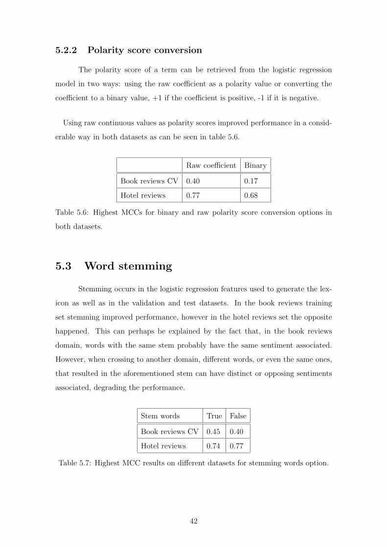
5.2.2 Polarity score conversion

The polarity score of a term can be retrieved from the logistic regression

model in two ways: using the raw coefficient as a polarity value or converting the

coefficient to a binary value, +1 if the coefficient is positive, -1 if it is negative.

Using raw continuous values as polarity scores improved performance in a consid-

erable way in both datasets as can be seen in table 5.6.

Raw coefficient Binary



Table 5.6: Highest MCCs for binary and raw polarity score conversion options in

both datasets.

5.3 Word stemming

Stemming occurs in the logistic regression features used to generate the lex-

icon as well as in the validation and test datasets. In the book reviews training

set stemming improved performance, however in the hotel reviews set the opposite

happened. This can perhaps be explained by the fact that, in the book reviews

domain, words with the same stem probably have the same sentiment associated.

However, when crossing to another domain, different words, or even the same ones,

that resulted in the aforementioned stem can have distinct or opposing sentiments

associated, degrading the performance.

Stem words True False



Table 5.7: Highest MCC results on different datasets for stemming words option.

42

5.4 SO-CAL parameters


Adjusting negative words to have a higher score increases performance when

testing against data from another domain. However, when used in the same domain,

it lowers MCC.

The decreasing in performance on same domain data may be explained by the

fact that the logistic regression model already takes into account the relevance and

rarity of each term’s sentiment, expressed by the continuous value in the coefficient.

Since most terms in this domain are already covered by the lexicon, when classifying

novel data in the same domain the negative terms that appear are already in the

lexicon with their rarity reflected on their polarity score. Applying a bias correction

is redundant and ends up degrading performance.

Whereas in a different domain negative words that are not part of the lexicon ap-

pear more frequently and don’t have their rarity taken into account. The coefficients

of negative words in the lexicon are not sufficient to reflect the rarity of negative

words in both domains, so using a positive bias normalization yielded better results.

Table 5.8 shows these results.

Normalize pos. bias True False



Table 5.8: Highest MCC results on different datasets for positive bias normalization

option.

5.5 Optimal hyperparameters combination

After analyzing individually how each hyperparameter affects the generated

lexicon in terms of performance, an optimal combination of hyperparameters that

maximize MCC was obtained for each dataset, the book reviews training set and the

43

hotel reviews dataset. Table 5.9 shows the combination of parameters that better

performed when tested against the book reviews training set, with cross-validation,

and when testing against the other domain set, namely the hotel reviews dataset.

The table also show the MCC and accuracy for each of them.

Book reviews CV Hotel reviews

Use valence shifters True False

Max. steps 4 -

Use balanced class weights True True

Remove stop words False True

Threshold 0.00 0.60

Polarity score conversion Raw coef. Raw coef.

Stem words True True

Normalize pos. bias False False

MMC 0.45 0.78

ACC 0.81 0.91

Table 5.9: Optimized combination of hyperparameters for each dataset along with

MMC and accuracy.

The hyperparameters that differentiate the two lexicons is the threshold value,

which is directly related to how fitted to data the generated lexicon will be, the use

of valence shifters and the removal of stop words as already noted in the individual

hyperparameters analysis.

5.6 Comparison against other sentiment lexicons

Although natural language processing as a whole is not as actively developed

in Portuguese as it is in English, some of the research effort in the area developed

and turned public sentiment lexicons for the Portuguese language.

Oplexicon [63] is a lexicon of 32192 terms. It is the larger publicly available lexicon

for the Portuguese language. The terms are emoticons, hashtags and words with

44

their respective POS tags and the polarities are -1 for negative sentiment bearing

words, +1 for positive ones and 0 for neutral words.

Sentilex [64] is comprised of mainly adjectives in a total of 7014 terms classified

as positive (+1) or negative (-1). In addition to individual words it also contains a

number of phrases. There are also neutral words in the lexicon but they are a small

part of it.

The ReLi lexicon [52] is a manually annotated sentiment lexicon that was built

on top of the same ReLi book reviews dataset used to generate our lexicon. It

is comprised of 519 polarized words accompanied by their POS tags and polarity

scores of -1 or +1. No neutral words are present in it. Being built on top of the

same data as our lexicon, it would be expected that both produced a lexicon with

similar performance.

None of the existing sentiment lexicons in Portuguese has any indicator on the

degree or intensity of the associated sentiment. They are simply labeled as positive

or negative, and in some cases neutral. The fact that this project’s generated lexicon

assigns polarity scores with varying degrees of intensity to terms can pose itself as

an advantage over the other ones.

Table 5.10 shows some structural information regarding the sentiment lexicons

used in this project. Book lexicon is the lexicon generated from the book reviews

corpus whose hyperparameters are optimized by testing against the same dataset

using cross-validation. Hotel lexicon is also generated from the book reviews

corpus but its hyperparameters were optimized by testing against the hotel reviews

dataset. In both lexicons stemmed terms are used since they presented a better

performance.

Tables 5.11 compares the performance of the SO-CAL method using each

sentiment lexicon when tested against the book reviews test set, it also presents the

lexicons size, only considering polarized terms. Table 5.12 compares performance in

tests against the hotel reviews dataset.

45

No. of positive terms No. of negative terms

Book lexicon 2253 130

Hotel lexicon 974 180

Oplexicon 8620 14569

Sentilex 1548 4598

ReLi lexicon 329 190

Table 5.10: Number of positive and negative terms in each sentiment lexicon.

Book reviews test set Size ACC MCC

Book lexicon 3227 0.83 0.52

Hotel lexicon 310 0.66 0.30

Oplexicon 22273 0.53 0.08

Oplexicon with stemming 8749 0.37 0.02

Sentilex 6132 0.37 -0.19

Sentilex with stemming 5163 0.47 0.09

ReLi lexicon 509 0.52 -0.02

ReLi lexicon with stemming 454 0.69 0.19

Table 5.11: Performance and size of each lexicon when tested against the book

reviews test set.

Hotel reviews dataset Size ACC MCC

Book lexicon 3227 0.71 0.51

Hotel lexicon 310 0.90 0.77

Oplexicon 22273 0.86 0.67

Oplexicon with stemming 8749 0.78 0.50

Sentilex 6132 0.82 0.59

Sentilex with stemming 5163 0.80 0.49

ReLi lexicon 509 0.70 0.47

ReLi lexicon with stemming 454 0.71 0.52

Table 5.12: Performance and size of each lexicon when tested against the hotel

reviews dataset.

46

The comparison showed that the generated lexicon had the best performance by

far when tested on data from the same domain it was trained on. As expected that

same lexicon didn’t perform quite as well in another domain but it managed to stay

around the average performance of other tested general purpose lexicons.

When optimized for another domain corpus, the generated lexicon had the best

performance in hotel reviews. Which indicates that a correct manipulation of hyper-

parameters can generate an efficient general purpose lexicon, at least for the domain

analyzed in this project. Overall, the performance was better on hotel reviews

dataset across all lexicons, revealing that it is an easier dataset to classify.

The generated lexicons were small in size when compared to others. However, if a

larger amount of data is available the vocabulary size should grow and consequently

the lexicon size.

Oplexicon performed well on hotel reviews, which can be due to the fact that

hotel reviews are more informal than book reviews. Since Oplexicon was based on

Twitter posts the formality of language may be similar to hotel reviews. Sentilex,

as well as all other lexicons did not perform well on the book reviews test set. Even

the ReLi lexicon, that was built on top of the same book reviews as the generated

lexicon performed poorly on this dataset.

47

Chapter 6

Conclusion

Using a logistic regression model to generate a sentiment lexicon proved to be a

reliable way of creating a lexicon. When optimized for an tested on the same do-

main, and when optimized and tested on a different domain, the generated lexicon’s

performance is superior to all other Portuguese sentiment lexicons publicly available

for the datasets analysed. As a downside, like other supervised methods, this kind

of lexicon requires a labeled dataset, which may not always be an available option.

The generated lexicon is corpus-based and domain specific, which means that it

can capture a sentiment for a word that only exists in a specific context. This is de-

sirable if the interest relies on classifying sentiment of texts in the same domain, but

when working in different domains this specific sentiment may lead to misleading

results. However, by using the threshold value, an attempt to build a more general

purpose lexicon can be made. In the tested case, using higher thresholds in combi-

nation with some other hyperparameters changes, the observed performance on data

from another domain was higher than other general purpose sentiment lexicons.

This project also validated some intuitions about parameters that could improve

or undermine the lexicon quality. For instance, using valence shifters as a prepro-

cessing step for features proved to be an effective way of raising the quality of the

lexicon. Using the model’s coefficients as polarity scores was also a measure that

improved performance. Usually binary values are used to express sentiment in man-

ually annotated lexicons for simplicity. Having continuous values instead for the

polarity scores increased performance when compared to simple binary labels in all

48

other tested lexicons.

6.1 Future Work

To further validate the hypothesis and extend it, a larger number of labeled

datasets can be used both for the generation as a training set as well as for the

evaluation process. Another possibility in the attempt to improve the lexicon is to

only use words from a specific part-of-speech type in the logistic regression model,

only adjectives and nouns for example, instead of using all terms to train the model.

Spelling correction could be used as a preprocessing step for features. The gen-

erated lexicon could also be expanded by dictionary-based methods and have any

discrepancy fixed in a one time manual inspection.

As extensions to SO-CAL’s valence shifters more sophisticated semantic rules can

be created and a higher number of modifiers values can be tested in an attempt to

find optimal ones. Locutions and expressions can be accepted as valence shifters.

The logistic regression model was used in this project to extract coefficients but

other supervised learning algorithms, like Support Vector Machines, could be used

as long as they associate a numeric value to each feature that this value somehow

correlates to the sentiment attribution.

If a huge number of labeled datasets are available, building a general purpose

lexicon can be attempted. Being those labeled datasets from different domains,

when training the model only relevant terms from all domains would have a high

coefficient and therefore have a prior polarity necessary in the process of making a

general purpose sentiment lexicon.

49

Bibliography

[1] Wikipedia, the free encyclopedia, “Random data points and their linear regres-

sion”, 2010, [Online; accessed September 1, 2016].

[2] Snider, Dallas, “Logistic Regression example”, 2015, [Online; accessed Septem-

ber 2, 2016].

[3] LIU, B., Sentiment Analysis and Opinion Mining, Synthesis Lectures on Human

Language Technologies. Morgan & Claypool Publishers, 2012.

[4] LIU, B., Sentiment analysis: Mining opinions, sentiments, and emotions. Cam-

bridge University Press, 1 2015.

[5] OSGOOD, C. E., SUCI, G., TANNENBAUM, P., The measurement of mean-

ing. Urbana, IL, University of Illinois Press, 1957.

[6] PANG, B., LEE, L., “Opinion Mining and Sentiment Analysis”, Found. Trends

Inf. Retr., v. 2, n. 1-2, pp. 1–135, Jan. 2008.

[7] LYONS, J., Language and Linguistics: An Introduction, Cambridge textbooks

in linguistics. Cambridge University Press, 1981.

[8] Langacker, R. W., “Observations and speculations on subjectivity”. In:

Haiman, J. (ed.), Iconicity in Syntax, pp. 109–150, 1985.

[9] BIBER, D., FINEGAN, E., “Adverbial stance types in English”, Discourse

Processes, v. 11, n. 1, pp. 1–34, 1988.

[10] CONRAD, S., BIBER, D., “Adverbial marking of stance in speech and writing”.

In: Hunston, S., Thompson, G. (eds.), Evaluation in Text: authorial stance and

the construction of discourse, Oxford, England, Oxford University Press, pp.

56–73, 2000.

50

[11] WIEBE, J. M., “Tracking Point of View in Narrative”, Computational Linguis-

tics, v. 20, pp. 233–287, Jun. 1994.

[12] SCHEIBMAN, J., Point of View and Grammar: Structural Patterns of Sub-

jectivity in American English Conversation, Studies in discourse and grammar.

John Benjamins Pub., 2002.

[13] HU, M., LIU, B., “Mining and Summarizing Customer Reviews”. In: Pro-

ceedings of the Tenth ACM SIGKDD International Conference on Knowledge

Discovery and Data Mining, KDD ’04, pp. 168–177, New York, NY, USA, 2004.

[14] PANG, B., LEE, L., VAITHYANATHAN, S., “Thumbs Up?: Sentiment Clas-

sification Using Machine Learning Techniques”. In: Proceedings of the ACL-02

Conference on Empirical Methods in Natural Language Processing - Volume 10,

EMNLP ’02, pp. 79–86, Stroudsburg, PA, USA, 2002.

[15] TURNEY, P. D., “Thumbs Up or Thumbs Down? Semantic Orientation Ap-

plied to Unsupervised Classification of Reviews”, CoRR, v. cs.LG/0212032,

2002.

[16] TABOADA, M., BROOKE, J., TOFILOSKI, M., et al., “Lexicon-based Meth-

ods for Sentiment Analysis”, Comput. Linguist., v. 37, n. 2, pp. 267–307, Jun.

2011.

[17] LU, Y., CASTELLANOS, M., DAYAL, U., et al., “Automatic construction of a

context-aware sentiment lexicon: an optimization approach”. In: Proceedings of

the 20th international conference on World wide web, WWW ’11, pp. 347–356,

New York, NY, USA, 2011.

[18] JOACHIMS, T., “Advances in Kernel Methods”. chapter Making Large-scale

Support Vector Machine Learning Practical, Cambridge, MA, USA, MIT Press,

pp. 169–184, 1999.

[19] CRISTIANINI, N., SHAWE-TAYLOR, J., An introduction to support vector

machines and other kernel-based learning methods. Cambridge University Press,

2000.

51

[20] FENG, S., ZHANG, L., LI, B., et al., “Is Twitter A Better Corpus for Measuring

Sentiment Similarity?” In: EMNLP, pp. 897–902, 2013.

[21] KIM, S.-M., HOVY, E., “Determining the Sentiment of Opinions”. In: Pro-

ceedings of the 20th International Conference on Computational Linguistics,

COLING ’04, Stroudsburg, PA, USA, 2004.

[22] KENNEDY, A., INKPEN, D., “Sentiment Classification of Movie Reviews Us-

ing Contextual Valence Shifters”, Computational Intelligence, v. 22, pp. 2006,

2006.

[23] TABOADA, M., GILLIES, M. A., MCFETRIDGE, P., “Sentiment Classifi-

cation Techniques for Tracking Literary Reputation”. In: LREC Workshop:

Towards Computational Models of Literary Analysis, pp. 36–43, 2006.

[24] POLANYI, L., ZAENEN, A., “Contextual Valence Shifters”. In: Working

Notes — Exploring Attitude and Affect in Text: Theories and Applications

(AAAI Spring Symposium Series), 2004.

[25] MILLER, G. A., “WordNet: A Lexical Database for English”, Commun. ACM,

v. 38, n. 11, pp. 39–41, Nov. 1995.

[26] VALITUTTI, R., “WordNet-Affect: an Affective Extension of WordNet”. In:

In Proceedings of the 4th International Conference on Language Resources and

Evaluation, pp. 1083–1086, 2004.

[27] BLAIR-GOLDENSOHN, S., NEYLON, T., HANNAN, K., et al., “Building a

sentiment summarizer for local service reviews”. In: In NLP in the Information

Explosion Era, 2008.

[28] ZHU, X., GHAHRAMANI, Z., “Learning from labeled and unlabeled data with

label propagation”, 2002.

[29] RAO, D., RAVICHANDRAN, D., “Semi-supervised Polarity Lexicon Induc-

tion”. In: Proceedings of the 12th Conference of the European Chapter of the

Association for Computational Linguistics, EACL ’09, pp. 675–682, Strouds-

burg, PA, USA, 2009.

52

[30] ESULI, A., SEBASTIANI, F., “Determining the Semantic Orientation of Terms

Through Gloss Classification”. In: Proceedings of the 14th ACM International

Conference on Information and Knowledge Management, CIKM ’05, pp. 617–

624, New York, NY, USA, 2005.

[31] ESULI, A., SEBASTIANI, F., “SENTIWORDNET: A publicly available lexi-

cal resource for opinion mining”. In: In Proceedings of the 5th Conference on

Language Resources and Evaluation (LREC’06, pp. 417–422, 2006.

[32] HATZIVASSILOGLOU, V., MCKEOWN, K. R., “Predicting the Semantic Ori-

entation of Adjectives”. In: Proceedings of the 35th Annual Meeting of the As-

sociation for Computational Linguistics and Eighth Conference of the European

Chapter of the Association for Computational Linguistics, ACL ’98, pp. 174–

181, Stroudsburg, PA, USA, 1997.

[33] ZHUANG, L., JING, F., ZHU, X.-Y., “Movie Review Mining and Summariza-

tion”. In: Proceedings of the 15th ACM International Conference on Informa-

tion and Knowledge Management, CIKM ’06, pp. 43–50, New York, NY, USA,

2006.

[34] CHOI, Y., CARDIE, C., “Adapting a Polarity Lexicon using Integer Linear

Programming for Domain-Specific Sentiment Classification.” In: EMNLP, pp.

590–598, 2009.

[35] JIJKOUN, V., DE RIJKE, M., WEERKAMP, W., “Generating Focused Topic-

specific Sentiment Lexicons”. In: Proceedings of the 48th Annual Meeting of the

Association for Computational Linguistics, ACL ’10, pp. 585–594, Stroudsburg,

PA, USA, 2010.

[36] COX, D. R., “The regression analysis of binary sequences (with discussion)”,

J Roy Stat Soc B, v. 20, pp. 215–242, 1958.

[37] MADSEN, H., THYREGOD, P., Introduction to General and Generalized Lin-

ear Models, Chapman & Hall/CRC Texts in Statistical Science. Taylor & Fran-

cis, 2010.

53

[38] PAMPEL, F., Logistic Regression: A Primer, Logistic Regression: A Primer.

SAGE Publications, 2000.

[39] ENGEL, J., “Polytomous logistic regression”, Statistica Neerlandica, v. 42,

pp. 233–252, 1988.

[40] MENARD, S., Applied Logistic Regression Analysis, n. no. 106 in Applied Lo-

gistic Regression Analysis. SAGE Publications, 2002.

[41] LIU, D. C., NOCEDAL, J., “On the Limited Memory BFGS Method for Large

Scale Optimization”, Math. Program., v. 45, n. 3, pp. 503–528, Dec. 1989.

[42] HARRIS, Z., “Distributional Structure”, Word, v. 10, n. 23, pp. 146–162, 1954.

[43] RAJARAMAN, A., ULLMAN, J. D., Mining of Massive Datasets. New York,

NY, USA, Cambridge University Press, 2011.

[44] BRUCE, R. F., WIEBE, J. M., “Recognizing Subjectivity: A Case Study in

Manual Tagging”, Nat. Lang. Eng., v. 5, n. 2, pp. 187–205, Jun. 1999.

[45] TABOADA, M., GRIEVE, J., “Analyzing Appraisal Automatically”. In: Pro-

ceedings of AAAI Spring Symposium on Exploring Attitude and Affect in Text

(AAAI Technical Report SS-04-07), pp. 158–161, 2004.

[46] SAVARESE, P. H. P., “Sentiment Analysis for Portuguese”,

https://github.com/lolemacs/portuguese-so-cal, 2015.

[47] QUIRK, R., GREENBAUM, S., LEECH, G., et al., A Comprehensive Grammar

of the English Language. London, Longman, 1985.

[48] SAURI, R., A Factuality Profiler for Eventualities in Text. Ph.D. dissertation,

Waltham, MA, USA, 2008. AAI3304029.

[49] DING, X., LIU, B., ZHANG, L., “Entity Discovery and Assignment for Opinion

Mining Applications”. In: Proceedings of the 15th ACM SIGKDD International

Conference on Knowledge Discovery and Data Mining, KDD ’09, pp. 1125–

1134, New York, NY, USA, 2009.

54

[50] SNIDER, J., OSGOOD, C., Semantic differential technique; a sourcebook. Al-

dine Pub. Co., 1969.

[51] VOLL, K., TABOADA, M., “Not all words are created equal: Extracting se-

mantic orientation as a function of adjective relevance”, AI 2007: Advances in

Artificial Intelligence, pp. 337–346.

[52] FREITAS, C., MOTTA, E., MILIDIU, R., et al., “Sparkle Vampire LoL! An-

notating opinions in a book review corpus”. In: 11th Corpus Linguistics Con-

ference, 2013.

[53] KING, G., ZENG, L., “Logistic Regression in Rare Events Data”, Political

Analysis, v. 9, n. 2, pp. 137–163, 2001.

[54] YU, H.-F., HUANG, F.-L., LIN, C.-J., “Dual Coordinate Descent Methods for

Logistic Regression and Maximum Entropy Models”, Mach. Learn., v. 85, n.

1-2, pp. 41–75, Oct. 2011.

[55] ALVARES, R. V., GARCIA, A. C. B., FERRAZ, I. N., “STEMBR: A Stemming

Algorithm for the Brazilian Portuguese Language.” In: Bento, C., Cardoso, A.,

Dias, G. (eds.), EPIA, v. 3808, Lecture Notes in Computer Science, pp. 693–701,

2005.

[56] COHEN, J., “A Coefficient of Agreement for Nominal Scales”, Educational and

Psychological Measurement, v. 20, n. 1, pp. 37–46, Apr. 1960.

[57] POWERS, D. M. W., “What the F-measure doesn’t measure: Features, Flaws,

Fallacies and Fixes”, CoRR, v. abs/1503.06410, 2015.

[58] RIJSBERGEN, C. J. V., Information Retrieval. 2 ed. Newton, MA, USA,

Butterworth-Heinemann, 1979.

[59] KENT, A., BERRY, M. M., LUEHRS, JR., F. U., et al., “Machine Litera-

ture Searching VIII. Operational Criteria for Designing Information Retrieval

Systems”, American Documentation, v. 6, n. 2, pp. 93–101, 1955.

[60] MATTHEWS, B. W., “Comparison of the predicted and observed secondary

structure of T4 phage lysozyme”, Biochimica et Biophysica Acta, v. 405,

pp. 442–451, 1975.

55

[61] POWERS, D. M. W., “Evaluation: From precision, recall and f-measure to

roc., informedness, markedness & correlation”, Journal of Machine Learning

Technologies, v. 2, n. 1, pp. 37–63, 2011.

[62] DEVIJVER, P. A., KITTLER, J., Pattern Recognition: A Statistical Approach.

London, Prentice-Hall International, Inc., 1982.

[63] SOUZA, M., VIEIRA, R., BUSETTI, D., et al., “Construction of a Portuguese

Opinion Lexicon from multiple resources”. In: In 8th Brazilian Symposium in

Information and Human Language Technology - STIL, Mato Grosso, 2011.

[64] “SentiLex-PT 02”, On request, 2012.

56

SENTIMENT LEXICON GENERATION WITH CONTINUOUS … · sentiment lexicon generation with continuous...

Documents

Transcript of SENTIMENT LEXICON GENERATION WITH CONTINUOUS … · sentiment lexicon generation with continuous...