1

Sentencing guidelines, judicial discretion and pleabargaining

Jennifer F. Reinganum*

The United States Sentencing Commission was created to develop federal sentencing guidelines, which

restrict judicial discretion and were found to increase the average sentence length while leaving

unchanged the likelihood of resolution through plea bargaining. A game theoretic model is developed in

which a sentencing commission may impose guidelines or defer to judicial discretion; then a defendant

and a prosecutor engage in plea bargaining; finally, those cases that fail to settle go to trial, where a

sentence is determined according to the guidelines, if imposed, or, if not, according to judicial

discretion. Equilibrium behavior is consistent with the aforementioned findings.

* Department of Economics, Vanderbilt University, Nashville, TN 37235jennifer.f.reinganum@vanderbilt.edu

I would like to thank Andrew F. Daughety for extensive conversations and thoughtful comments toonumerous to mention. Also thanks to the Editor-in-Chief, the referees, Jennifer Arlen, Mark Cohen, JamesFoster, Luke Froeb, Daniel Kessler, Tracy Lewis, Preston McAfee, Richard Posner, David Sappington,Eric Talley and seminar participants at the 1997 American Law and Economics Association meetings, the1997 NBER Summer Institute on Law and Economics, Penn State University, Washington University andthe University of Southern California for many helpful remarks. The financial support of NSF Grant No.SBR-9596193 is gratefully acknowledged.

2

1. Introduction

When one level of a hierarchy devises rules for a sub-level, conflict can arise even if both levels are

in full agreement about the goals of the hierarchy. The source of this conflict is the timing of the decisions

that the rules affect and the availability of information that the timing implies. A good example of this

conflict is the one which arose between the United States Sentencing Commission (hereafter USSC) and the

federal judiciary concerning sentencing guidelines which restrict the exercise of judicial discretion1 in

sentencing.

In this paper, the USSC and the federal sentencing guidelines are described. Empirical

characterizations of the impact of the guidelines on sentence length and plea bargaining, as assessed by the

USSC, are presented. A hierarchical model of sentencing is then developed in which a sentencing

commission, prosecutors, defendants and judges all interact. Although the sentencing commission and the

judges agree about the goal being pursued, differences in timing and information lead them to make

different decisions regarding sentencing. The equilibrium implications of the model are consistent with the

aforementioned empirical characterizations.

The Sentencing Reform Act of 1984 delegated to the USSC (an independent agency in the judicial

branch of government) the authority to review and “rationalize” the federal sentencing process and, in

particular, to develop detailed guidelines specifying appropriate sentences for offenders convicted of federal

crimes. These guidelines prescribe a range of sentences based on characteristics of the offense and the

offender, leaving a narrow margin of judicial discretion within the prescribed sentence range.2 If the court

wishes to sentence outside this range, it must detail its reasons, and such deviations (referred to by the

USSC as “departures”) can be appealed by either side. The Act also abolishes parole, so that the sentence

given is the sentence served (with small reductions for good behavior).

3

According to Freed (1992, p. 1719), groups such as the Judicial Conference of the United States

and the American Bar Association favored delaying the imposition of guidelines until legislative hearings

could be held. However, Congress did not take this advice, and the guidelines went into effect in 1987.

Lawsuits challenging the constitutionality of the guidelines followed, but the Supreme Court upheld the

constitutionality of the guidelines by an eight-to-one vote in the case of Mistretta v. United States in 1989.

The USSC was given the on-going task of monitoring federal sentencing practices and revising the

guidelines as the need arises.

The motivation for such guidelines included at least the following arguments. First, the then-

current system of indeterminate sentencing with parole made it difficult for either the offender or the state

to form a reasonable estimate of the actual sentence; definitive sentencing guidelines were believed to

provide honesty in sentencing. Second, the sentencing guidelines were intended to reduce observed

disparity in sentencing across apparently similar cases. Finally, the sentencing guidelines would build in

proportionality in sentencing by conditioning the prescribed sentence on offense and offender

characteristics. The USSC asserted that these desiderata could be supported either by reference to the

principle of “just deserts” or to the principle of deterrence, so it did not take a particular philosophical

approach to enforcement.

In an attempt to provide continuity while reducing disparity, for most offenses the guideline range

was centered on the previous average sentence. This mechanical procedure does not guarantee that the

average sentences before and after the guidelines will be equal, even ignoring the potential impact of

guidelines on the selection of cases coming to trial. For some offenses, notably those involving drugs and

guns, the guidelines incorporated many mandatory minimum sentences3 contained in laws enacted by

Congress. For some property crimes, there was a deliberate move to reduce the use of probation in favor of

shorter, but more certain, periods of incarceration. Finally, some penalties were raised to maintain

consistency; for instance, Jeffrey S. Parker and Michael K. Block, a former member of the USSC (1989,

4

p. 315), say that “increases in antitrust sentences were intended to rationalize antitrust offenses with fraud

offenses, on the premise that many criminal antitrust offenses, which predominantly involve bid-rigging, are

a form of fraud.”

The guidelines are widely perceived to provide harsher penalties than would occur under judicial

discretion, in part because of the aforementioned structural changes and in part due to extremely negative

initial judicial reaction (see Freed, 1992, for examples). If this perception that the guidelines provide

harsher sentences than had previously occurred (or would occur) under judicial discretion is correct, then it

should be the case that average sentence lengths have increased under the guidelines. The increase in mean

sentence length since the adoption of the guidelines is documented in USSC Table D-13 (1991, p. D-13).

Using monthly data from July 1984 to June 1990, the USSC regressed mean sentence on dummy variables

for four interventions which might be expected to affect sentence lengths: the Anti-Drug Abuse Act of

1986 (ADAA86), the Anti-Drug Abuse Act of 1988 (ADAA88), the implementation of the guidelines (in

1987) and the Mistretta decision (in 1989). They found that all but ADAA88 had a positive and

significant effect on mean sentence length, and an increase in average sentence length of 8.19 months was

attributed to the combined effects of guideline implementation and the Mistretta decision (USSC Table

137, 1991, p. 372). Separate analyses were conducted for drug offenses (Table D-15) and for robbery

(Table D-17), with similar results: both the guidelines and the Mistretta decision had positive and

significant effects on mean sentence length (with a combined increase of 7.7 months for drug offenses and

14.78 months for robbery; see Table 137). Mean sentence lengths for economic crimes4 (taken as a group)

were found to be stable over this time period (the coefficients were positive but insignificant).

Further evidence that the guidelines impose higher sentences than would occur under judicial

discretion involves an assessment of sentence placement within the guideline range and the direction and

extent of departures from the guideline range. USSC Table 32 (1995a) reports that during the time period

October 1, 1994 - September 30, 1995, 91.9% of all federal criminal convictions involved a guilty plea

5

and 66.1% of all federal sentences fell within the guideline range. The range is divided into quarters, with

44.1% of all sentences falling into the first quarter of the guideline range, 9.2% falling into the second

quarter, 3.5% falling into the third quarter and 9.3% falling into the fourth quarter. Of course, there is

substantial variation across different offenses, but the pattern is distinctly “clumped” toward the lower end

of the range (even for economic crimes such as larceny, fraud, embezzlement, counterfeiting, tax evasion

and money laundering), which is consistent with a desire to give a lower sentence in some cases but being

constrained to sentence within the guideline range.

The remaining cases represent departures from the guidelines, with 23% of cases involving a

downward departure based on the offender having provided “substantial assistance” to the prosecutor (such

departures are authorized by the sentencing guidelines) and 9.8% of cases involving a downward departure

for other reasons; only 1.1% of cases involved an upward departure. Moreover, since plea bargaining can

result in conviction on a lesser charge (with a correspondingly lower guideline sentencing range), some of

the sentences that fell within the guideline range are likely to represent informal downward departures.

The same report documenting the positive impact of the guidelines on sentence length finds no

impact of the guidelines or Mistretta on the likelihood of trial (USSC 1991, p. 410). “Of particular interest

is the lack of an effect associated with the guidelines on the number and proportion of guilty pleas among

filed cases. This finding stands in stark contrast to the prediction by some that the guidelines would cause

(or have caused) an increase in the rate of defendants going to trial. To the contrary, the data analyses

support the conclusion that this has not happened. If the number of trials has increased, it is due to the fact

that more cases are being filed; the rate of defendants’ choosing to enter guilty pleas or stand trial has not

changed appreciably as a result of guideline implementation.”

Several different measures are reported as reflecting the plea rate. First, the ratio of guilty pleas to

cases resolved (either by plea or by trial) can be found from data reported in USSC Table 138 (1991, p.

397) for the years 1984 through 1989. This series is: 88.2%, 88.2%, 85.5%, 86.2%, 85.3% and 87.3%,

6

where the first three numbers refer to the pre-guidelines regime and the last three numbers refer to the post-

guidelines regime. There does not appear to be any perceptible impact in this brief series. Second, the

ratio of guilty pleas to cases filed is used in a time series analysis using monthly data from October 1986

through March 1990, reported in USSC Table E-12 (1991, p. E-12). Neither the guidelines

implementation nor the Mistretta decision had a statistically significant impact on the plea rate. Finally,

the ratio of guilty pleas to convictions (usually referred to as the “mode of conviction”) is depicted in USSC

Figures 24-26 (1991, pp. 407-409) for drug cases, robbery cases and all cases, respectively, over the same

time period using monthly observations. Again there is no discernible impact of either the guidelines

implementation or the Mistretta decision.5

The USSC recognized (the discussion in this paragraph is based on USSC 1995b, p. 5.) that

prosecutorial discretion could be problematical, especially since prosecutors’ behavior is difficult to

observe. The charge offense system that was adopted, in which the guidelines specify a sentence based on

the offense for which the offender is indicted and convicted (rather than his actual behavior6) gives

prosecutors the ability to influence sentencing by increasing or decreasing the seriousness and/or number of

charges in the indictment. Although there is a limit to how much the prosecutor can increase the sentence

(since the charges must ultimately be proved), the prosecutor’s ability to decrease the sentence in exchange

for a guilty plea does not appear to be substantially limited, especially since charge bargaining may be used

very early in the process. The sentencing court must verify that the proposed sentence is within the

guidelines for the offense charged, but prosecutorial discretion7 is otherwise largely unaffected. The

prosecutor and the defense attorney can jointly determine the charges, and sometimes even the facts (e.g.,

the weight or type of drug involved, whether or not a gun was used), thus determining the guideline

sentencing range within which the court will operate.

In this paper, a model of criminal sentencing is developed which compares judicial discretion with

sentencing guidelines. It will be assumed that the court and the sentencing commission are in agreement

7

regarding the desirability of honesty and proportionality in sentencing. Thus, assume that there is a single

offense of variable severity (where severity may depend upon offense and offender characteristics). For

each level of severity, there is an ideal sentence, about which the court and the sentencing commission are

in complete agreement. Moreover, assume that both the court and the sentencing commission are motivated

by the desire to minimize the expected squared error between the ideal and the actual sentence imposed in

any given case: that is, both the court and the sentencing commission are interested in case-by-case

justice.8 Thus, if perfect information about the offense and the offender were available at the time of

sentencing, the court and the sentencing commission would have no disagreement regarding the optimal

sentence. However, if perfect information about the offense or the offender is not available at the time of

sentencing, then the sentence can be determined either (a) by judicial discretion, in which case the optimal

sentence is that which minimizes the expected squared error, conditional on all information available to the

court; or (b) by reference to the sentencing guidelines, which specify a sentence to apply under these

circumstances. These two regimes are compared and it is shown that the resulting sentences will differ.9

Disagreement between the court and the sentencing commission arises because of plea bargaining,

which occurs before trial and sentencing. Plea bargaining results in a biased selection of cases going to

trial, and it is this selection of cases that the court observes and decides. When perfect information about

the offense or the offender in a given case is unavailable at the time of sentencing, it is this posterior

distribution10 that the court uses to compute its “best guess” about the appropriate sentence. While

expectations about this sentence affect the plea bargaining phase (since it is the alternative to which any

plea bargain will be compared), the court does not have control over the sentence in cases that settle

through a plea bargain.11 On the other hand, the sentencing commission acts not at the time of sentencing,

but before any plea agreements are made. Thus, its objective function reflects not only errors in sentencing

which may occur at trial due to imperfect information, but also those that occur routinely as a result of plea

bargaining. The sentencing commission can commit to a sentence at trial (to be applied in the event of

8

imperfect information regarding the ideal sentence for a given case) which would be suboptimal ex post of

trial, but which provides better incentives to the prosecutor ex ante of trial, resulting in more appropriate

plea bargains.12 Thus, while it is assumed that the court and the sentencing commission agree in principle

about the ideal sentence for a given offense and offender, they act at different times and with different

information.

Suppose that the defendant has private information about the true severity of his crime (as

measured by his behavior during the offense and his prior criminal history and other characteristics), which

allows him to anticipate the sentence which will be imposed if trial reveals this information perfectly (e.g.,

through the actual trial or the pre-sentencing report). At the time of plea bargaining, the prosecutor knows

only the prior distribution over the offense and offender characteristics, and hence only the prior

distribution over the sentence in the event of trial. The court is assumed to observe a verifiable public

signal (i.e., the trial or pre-sentence report), which is either perfectly informative or perfectly

uninformative. If the signal is informative, then true severity is revealed and the court imposes the ideal

sentence. In theory, the sentencing commission could also specify a sentence which differs from the ideal

sentence in the event that the trial is informative. An unconstrained sentencing commission might choose to

do this to further manipulate the downstream plea bargaining stage. However, the sentencing commission

is not unconstrained; if there is general agreement about the ideal sentence for a crime of given severity and

the trial verifiably reveals that severity, we assume that the commission cannot impose a different sentence

(e.g., because the sentence will certainly be modified on appeal given the facts established at trial). Judicial

discretion or the sentencing commission’s default sentence can only be exercised if the facts of the case

remain ambiguous following trial.

If the signal is uninformative, then in a regime of sentencing guidelines the court will impose the

specified sentence, which is denoted xG (although the actual guidelines specify an interval, or sentence

range, if they are binding then it is only the binding endpoint that matters). If the signal is uninformative,

9

then in a regime of judicial discretion the court will impose its “best guess” about the ideal sentence, which

is denoted x J. The prosecutor and the defendant will have common knowledge of xG in a regime of

sentencing guidelines, but in the case of judicial discretion, the prosecutor and defendant will need to form a

conjecture about what sentence the court will impose. This common conjecture is denoted xC; in

equilibrium, this conjecture must be correct: xC = x J. It will prove economical to define the expression xT

to be the anticipated sentence following trial in the event the public signal (the trial) is uninformative. Then

T takes on the index G (in a regime of sentencing guidelines), C (in a regime of judicial discretion prior to

the court’s decision) or J (in a regime of judicial discretion after the court’s decision). Notice that judicial

discretion only comes into play when the trial itself is not decisive; even then, the court is minimizing its

expected squared sentencing error. Thus, judicial discretion in this model does not assume arbitrary, biased

or self-interested behavior on the part of the court.

A signaling game is considered in which the informed defendant makes a plea offer, which is

accepted or rejected by the prosecutor. Thus, the bargaining power lies with the defendant, who can take

advantage of the prosecutor’s desire to avoid trial costs to obtain a reduced sentence relative to what he

would receive at trial. In this case, the following results are obtained:

(1) the defendant’s plea offer is an increasing function of true severity and xT; that is,

defendants anticipating a higher sentence at trial make higher plea offers.

(2) the equilibrium probability of trial is a decreasing function of true severity and is

independent of xT; that is, cases involving greater severity are more likely to be resolved

by plea bargain.

(3) xG > x J; that is, the optimal sentence as specified by the sentencing guidelines exceeds

the court’s optimal sentence under judicial discretion.

10

It is interesting to compare the implications of these results with the USSC’s (1991) findings.

Result (3) implies that convicted offenders anticipate a longer expected sentence at trial under sentencing

guidelines than under judicial discretion. Result (1) implies that, as a consequence of result (3), defendants

make higher plea offers. Thus, regardless of the mode of conviction, the model predicts that the expected

sentence will be longer under sentencing guidelines, which is consistent with the data reported earlier on the

positive impact of sentencing guidelines on average sentence length. Finally, notice that result (2) implies

that the probability of trial is independent of the sentencing regime (guidelines versus judicial discretion) for

any given defendant, and thus the ex ante expected probability of trial among all defendants is also

independent of the sentencing regime. This is consistent with the USSC’s finding that the guidelines did not

have any discernible impact on the rate of defendants going to trial.

Next the intervening plea bargaining model is extended to a collection of crimes, each of variable

severity, but ordered in terms of “seriousness” in that crime j is more serious than crime i if the range of

severity for crime j is upward-shifted relative to that of crime i. Thus, murder is more serious than assault

because the maximum ideal sentence for murder exceeds that for assault. A further result is:

(4) the equilibrium probability of trial is an increasing function of the seriousness of the crime;

that is, cases involving more serious crimes are more likely to go to trial.

This is consistent with the intuition that more serious categories of crimes are less likely to be

resolved through a plea bargain, and the intuition itself is correct. In USSC Table 17 (1995a, p. 56), the

mode of conviction is broken down by primary offense category. Crimes in which conviction by plea

bargain is least likely are murder (67.9%), kidnapping/hostage-taking (79%) and assault (80.2); those in

which conviction by plea bargain is most likely are immigration (98.1%), embezzlement (98%) and

gambling/lottery violations (97.7%).

11

Finally, a number of robustness issues are discussed, including the impact of reversing the order of

play (i.e., a screening game in which the uninformed prosecutor makes the plea offer and the informed

defendant accepts or rejects the offer). Results (1) and (2) above continue to hold, but now examples can

be constructed to show that either xG > x J or xG < x J may hold. The latter outcome can arise in the

screening game because the prosecutor has the bargaining power; this can, but need not, result in the

sentencing commission constraining judicial discretion by specifying xG < x J.

In a technical appendix (available from the author upon request), a comparison is also made with

the case of imperfect, rather than asymmetric, information. In this case it is shown that the sentencing

commission still prefers to restrict judicial discretion, imposing xG > x J when the defendant makes the plea

offer and xG < x J when the prosecutor makes the offer. Alternative prosecutorial objective functions which

are more closely aligned with the sentencing commission’s objectives are also considered. Even when the

prosecutor is assumed to minimize the expected squared sentencing error, the incentive for the sentencing

commission to constrain the court remains. This occurs because the more severe cases remain more likely

to settle by plea bargain, inducing a difference between the prior distribution of cases and the posterior

distribution of cases handled by the court.

2. The basic model

We begin by assuming a particular offense, which is considered to vary in its severity based on

differences in the offender’s behavior and characteristics. For any given case, the severity of the offense,

indexed by the corresponding ideal sentence, is a random variable denoted X. The defendant is assumed to

know x, his realized value of X. The prosecutor knows only that X is distributed according to the

cumulative distribution function F(.), with density f(.), on the support [x, xGG ]. Finally, if a case goes to

12

trial, the court receives a verifiable public signal which is either perfectly informative (reveals x) or

perfectly uninformative.13 The probability that the public signal is uninformative is denoted , 0 (0,1], and

is assumed to be independent of the realized value of x.

The model is divided into three stages: commission decision-making, plea negotiations and

sentencing. In the first stage, the sentencing commission may determine a sentence, denoted xG, which

applies in those cases which come to trial and for which the public signal is uninformative, or it may leave

sentence determination in this event to judicial discretion; that is, the sentencing commission first chooses

the regime. Under judicial discretion, the sentence in the event that trial is uninformative will be based

upon all information available to the court at that time. This information consists of the prior distribution

F(.), the fact that the case came to trial rather than settling, and any inferences that may be drawn from the

latter observation. This information is also available to both the prosecutor and the defendant (and the

defendant’s private information does not give him any “edge” over the prosecutor in predicting the court’s

choice14), so it is assumed that they have a common conjecture xC about what sentence will be imposed by

the court in the event that the trial is uninformative.

In the second stage, the defendant and the prosecutor engage in plea negotiations. The model

assumes that all defendants are in fact guilty, so that any potential false accusations have already been

eliminated (see Reinganum, 1988, for a model in which prosecutors optimally drop cases against

defendants for whom the prosecutor’s prior probability of guilt is sufficiently low). For the moment,

conviction is assumed to be certain, but later we will consider an exogenous probability of conviction : <

1. In this section, we assume that the defendant makes a plea offer S to the prosecutor, who accepts or

rejects it; the alternative order of moves will be examined in Section 4. The defendant’s anticipated

sentence at trial in the event the public signal is uninformative is denoted xT. If the sentencing commission

has specified a sentence xG, then xT = xG. On the other hand, if sentencing in the event of an uninformative

signal has been left to judicial discretion, then xT = xC. The defendant would like to minimize his total loss,

13

which consists of the expected sentence plus expenditures on trial. Let kD denote the costs of trial to the

defendant (measured in sentence-equivalent terms; this may be very small in the case of an indigent

defendant represented by a public defender). If the defendant settles, his loss is simply S. But if he goes to

trial, his expected loss is given by (1 - ,)x + ,xT + kD. Thus, the defendant’s strategy consists of a plea

offer which may depend on x and xT, and is denoted S(x; xT).

Assume that the prosecutor, who considers each case on an individual basis, is motivated to obtain

long sentences and to hold down public expenditures on trial costs. For instance, an elected prosecutor may

maximize his chances of re-election by being “tough on crime” and “saving the taxpayers’ money.”

Although a federal prosecutor is not elected, he may have aspirations of holding elected (or appointed)

office in the future, or may gain other career advancement by being perceived to have done a good job as a

prosecutor, and so likewise wants to establish a similar record.

Thus, the prosecutor who settles for a sentence of S receives simply S, while a prosecutor who goes

to trial can expect (1 - ,)b(S; xT) + ,xT - kP, where kP is the cost of trial for the prosecutor (measured in

sentence-equivalent terms; in the case of an indigent defendant, kP might also include the cost of the public

defender) and b(S; xT) denotes the prosecutor’s beliefs: upon observing S, the prosecutor believes15 that he

is facing a defendant of type b(S; xT). A strategy for the prosecutor is a function r(S; xT), denoting the

prosecutor’s probability of rejecting the plea S. Given an equilibrium plea offer function S*(x; xT) and an

equilibrium probability of rejection function r*(S; xT), the equilibrium probability of trial as a function of x

and xT is D(x; xT) = r*(S*(x; xT); xT).

Notice that, whether xT is the conjectured sentence to be determined by the court at the time of

sentencing (judicial discretion) or whether it has already been specified by the sentencing commission

(sentencing guidelines), it is taken as exogenous by the prosecutor and the defendant. However, in the case

of judicial discretion it is the parties’ conjectured sentence at trial which is relevant to the plea bargaining

(and hence the court’s actual choice of this sentence, which occurs later, cannot influence the negotiation

14

stage) while in the case of sentencing guidelines it is the sentence specified in the first stage which is

relevant to the plea bargaining (and hence the specified sentence can influence the negotiation stage).

In the third stage, sentencing occurs. Sentences arising out of plea bargains are assumed to be

accepted by the court (with the prosecutor adjusting the charge, if necessary, to achieve consistency with

the guidelines by which the court is bound). Any case that has not settled goes to trial, generating a public

signal (which may or may not be informative) about its severity. If no discretion remains for the court (i.e.,

in the case of sentencing guidelines), then if the public signal is informative, x (the ideal sentence) is

revealed and the actual sentence is set equal to this ideal sentence, while if the public signal is

uninformative, then the court imposes the sentence xG as specified by the guidelines. Alternatively, in a

regime of judicial discretion, the court chooses a sentence so as to minimize the expected squared difference

between the ideal sentence and the actual sentence. Thus, if the public signal is perfectly informative, then

x is revealed and the actual sentence is set equal to this ideal sentence, while if the public signal is

uninformative, then the court chooses xT to minimize its payoff, denoted EA J , which is taken to be the

expected squared sentencing error EJ[ (X - xT)2 | trial ], where the superscript J on the expectation operator

indicates that the court uses its posterior beliefs about the distribution of X given that a case has come to

trial.

3. Analysis and results

The court’s problem

The problem will be analyzed in reverse order of the stages to assure subgame perfection. If the

court has any real choice at the time of sentencing, it is because the sentencing regime involves judicial

15

discretion. In this case, the behavior of the defendant and the prosecutor is contingent on xC, their common

conjecture about the sentence the court will impose if the public signal is uninformative. Let H(x; xC) be

the court’s beliefs, or posterior cumulative distribution function over X, given that trial has occurred. Note

that the court’s utility function is based only on the outcome in those cases in which it actually plays an

active role.16 This is for two reasons: first, these are the only cases in which the court’s decision can have

an impact, given its place in the hierarchy; second, it is plausible that these are the cases for which the

court feels directly responsible, and which would form the basis for any external evaluation of the court’s

performance (settled cases being the purview of the prosecutor). Then the court chooses xT to minimize

EA J(xT; xC) / EJ[ (X - xT)2 | trial ] = I(x - xT)2h(x; xC)dx,

where h(x; xC) is the density function for H(x; xC) and the integral is taken over the domain [x, xGG ]. In the

remainder of the analysis, whenever the domain of integration is not specified, it should be understood to be

[x, xGG ]. Notice that xC denotes the common conjecture on the part of the prosecutor and the defendant

regarding the sentence that will be imposed (in the event that the public signal is uninformative), while x J is

the actual sentence chosen by the court at the time of sentencing. Thus the best-response value of xT (given

the prosecutor and defendant’s common conjecture xC) is given by

BRJ(xC) = Ixh(x; xC)dx.

In equilibrium, all parties’ conjectures and beliefs must be correct. In particular,

h(x; xC) = D(x; xC)f(x)/ID(y; xC)f(y)dy and xC = x J. Thus the equilibrium value x J satisfies

x J = IxD(x; x J)f(x)dx/ID(y; x J)f(y)dy. (1)

Although the equilibrium court sentence under judicial discretion is related to the equilibrium

behavior of the prosecutor and the defendant as described in equation (1), all parties take the others’

strategies as given (since the prosecutor is choosing a best response to the defendant’s offer and to his

conjecture about the sentence the court will impose, the defendant is choosing a best response to the

16

prosecutor’s rejection strategy and to his conjecture about the sentence the court will impose, and the court

is choosing a best response to its beliefs about the distribution of cases coming to trial).

Plea negotiations

Now consider the second, or plea negotiations, stage. In this subsection, the summary notation xT

will be used throughout, since the analysis of this stage is the same whether xT has already been chosen by

the sentencing commission or whether it will be chosen later by the court. The unique revealing

equilibrium17 for this game will be characterized. Let A P(r, S; b(S; xT)) denote the expected utility to the

prosecutor when he rejects the plea offer of S with probability r, based on his beliefs b(S; xT). Then

A P(r, S; b(S; xT)) = (1 - r)S + r[(1 - ,)b(S; xT) + ,xT - kP].

Let A D(S, x; r(S; xT)) denote the expected disutility to the defendant of type x when he offers a plea of S,

given the prosecutor’s probability of rejection function r(S; xT). Then

A D(S, x; r(S; xT)) = (1 - r(S; xT))S + r(S; xT)[(1 - ,)x + ,xT + kD].

In a revealing equilibrium, each defendant type makes a distinct plea offer. Moreover,

r(S; xT) must be a decreasing function of S; that is, higher offers must be more likely to result in settlement

rather than trial. For if this were not the case, then two defendant types who are supposed to make the

distinct offers S1 and S2 would both pool at the lower offer, because it involves both a lower sentence and a

lower probability of rejection. This contradicts the hypothesis of revelation.

Since r(S; xT) must be a decreasing function of S, it is interior to the interval [0,1] for almost all

values of S. The prosecutor will be indifferent between accepting the plea offer S or going to trial if and

only if S = (1 - ,)b(S; xT) + ,xT - kP. Furthermore, by definition, a revealing equilibrium requires that

b(S*(x; xT); xT) = x. This further implies that S*(x; xT) = (1 - ,)x + ,xT - kP.

Finally, S*(x; xT) must minimize A D(S, x; r*(S; xT)). Differentiating with respect to S yields

17

MA D(S, x; r*(S; xT))/MS = 1 - r*(S; xT) + [Mr*(S; xT)/MS][(1 - ,)x + ,xT + kD - S] = 0.

Substituting S*(x; xT) = (1 - ,)x + ,xT - kP and simplifying gives the following first-order differential

equation defining r*(S; xT).

1 - r*(S; xT) + K[Mr*(S; xT)/MS] = 0, (2)

where K / kP + kD. There is a unique solution to this equation through any given boundary condition. In

this case, the appropriate boundary condition is r*( SGG; xT) = 0; that is, the highest offer observed in

equilibrium must be accepted with certainty. This is because it is a dominant strategy to accept any S > SGG,

since this is more than the prosecutor could ever expect at trial. Were the offer SGG not accepted with

certainty, the defendant type making it would offer just a little more, ensuring acceptance but violating the

hypothesis that SGG is an equilibrium offer. Thus r*( SGG; xT) = 0 in equilibrium. The unique solution to

equation (2) through this boundary condition is given by r*(S; xT) = 1 - exp{-( SGG - S)/K}. Combining the

equilibrium plea offer function18 S*(x; xT) and the equilibrium probability of rejection function r*(S; xT)

yields the equilibrium probability of trial function D(x; xT) = 1 - exp{-(1 - ,)( xGG- x)/K}.

Proposition 1. (a) The equilibrium plea offer is increasing in x and xT; that is, defendants anticipating a

higher sentence at trial make higher plea offers; (b) The probability that a defendant of type x goes to trial

is a decreasing function of x and is independent of xT.

The fact that D(x; xT) is independent of xT allows us to write the equilibrium probability of trial for

a defendant of type x as simply D(x) and the ex ante equilibrium probability of trial among all defendants as

ID(y)f(y)dy. Thus the equilibrium sentence under judicial discretion is

18

x J = IxD(x)f(x)dx/ID(y)f(y)dy. (3)

That is, x J is just the conditional mean of X among those cases that come to trial. Let x̂ = Ixf(x)dx denote

the unconditional mean of X. The proof of the following proposition can be found in the Appendix.

Proposition 2. The conditional mean among those cases that come to trial is less than the unconditional

mean; that is, x J < x̂ .

Thus, since more severe cases are more likely to settle through a plea bargain, the distribution of cases

facing the court19 is downward-biased relative to the prior.

Now consider a collection of crimes which are ordered in terms of “seriousness.” We will say that

crime j is more serious than crime i if xGGj > xGGi. For instance, murder and assault are two categories of

crimes. In general, murder is considered more serious than assault, though actual crimes within each

category can be of variable severity and the range of ideal sentences can involve a substantial overlap.

However, most would agree that the maximum ideal sentence for murder exceeds that for assault.

Differentiating D(x) = 1 - exp{-(1 - ,)( xGG - x)/K} with respect to xGG yields

MD(x)/M xGG = exp{-(1 - ,)( xGG - x)/K}(1 - ,)/K > 0. That is, for a given true severity x, the equilibrium

probability of trial is higher for defendants who have committed a more serious crime.

Finally, suppose that conviction is not guaranteed,20 but occurs with an exogenous probability

denoted :. It is straightforward to show that the equilibrium plea offer becomes S*(x; xT) = :(1 - ,)x +

:,xT - kP and the equilibrium probability of trial becomes D(x; xT) = 1 - exp{-:(1 - ,)( xGG - x)/K}. Thus

the equilibrium probability of trial remains independent of xT, though it increases with the likelihood of

conviction :; that is, cases which the prosecutor is more likely to win are more likely to go to trial.

19

The sentencing commission’s problem

Finally, consider the first stage, in which the sentencing commission chooses the regime; that is, it

can specify xT or delegate that decision to the court. It is assumed that the sentencing commission cares

about sentencing error (i.e., discrepancies between ideal and actual sentences) and about conserving trial

costs. However, since the probability of trial is independent of xT, the aggregate resources spent on trials,

KID(y)f(y)dy, will not be affected by whether xT is specified or delegated. Thus, consideration of trial costs

can be omitted without loss of generality.

The model will allow for different weights to be placed on sentencing errors introduced by plea

bargaining and sentencing errors introduced at trial by specifying the social loss function as a convex

combination of these errors (of course, the weights may be the same). The expected social loss arising

from sentencing errors at trial is the product of two terms: the expected number of trials and the expected

sentencing error conditional upon trial, denoted ESET(xT). The first of these terms is given by ID(y)f(y)dy,

while the second is the same as the court’s payoff function in the same circumstances.

ESET(xT) = EA J(xT) = I(x - xT)2D(x)f(x)dx/ID(y)f(y)dy. (4)

Notice that this function is minimized at xT = x J, and recall that x J < x̂ .

The expected social loss due to sentencing errors in cases settled by plea bargaining is also the

product of two terms: the number of cases settled and the expected sentencing error conditional on

settlement. The expected number of cases settled by plea is I(1 - D(y))f(y)dy and the expected sentencing

error conditional on settlement by plea bargain, denoted ESEB(xT), is

ESEB(xT) = I(x - S*(x; xT))2(1 - D(x))f(x)dx/I(1 - D(y))f(y)dy

= I(,(x - xT) + kP)2(1 - D(x))f(x)dx/I(1 - D(y))f(y)dy. (5)

This function is minimized at xB such that

20

xB = Ix(1 - D(x))f(x)dx/I(1 - D(y))f(y)dy + kP/,. (6)

The first term is the mean severity, conditional on the case having settled through plea negotiations. By an

argument analogous to the proof of Proposition 2, the following proposition can be proved.

Proposition 3. The conditional mean among those cases settling by plea is greater than the

unconditional mean; thus, by equation (6), xB > x̂ + kP/,.

The aggregate ex ante expected social loss, denoted ESL(xT), can be written as follows:

ESL(xT) = "[I(1 - D(y))f(y)dy]ESEB(xT) + (1 - ")[ID(y)f(y)dy]ESET(xT). (7)

This is a weighted average of two quadratic functions of xT; hence its minimum will occur at a value of xT

between those values of xT that minimize ESEB(xT) and ESET(xT), respectively. Let xG denote the optimal

guideline sentence to be imposed following a trial at which the public signal was uninformative.

Proposition 4. For " = 0, xG = x J; for " = 1, xG = xB; for " 0 (0, 1), xG 0 (x J, xB).

Although the court and the sentencing commission agree in their evaluation of errors in sentencing

following trials (and thus the sentencing commission would make the same decision as the court were their

roles in the hierarchy reversed), the sentencing commission can improve its objective by increasing the

sentences that arise out of plea bargains. It does this by setting a longer sentence at trial (in the event of an

uninformative public signal) than the court would choose were it given discretion.

Notice that there is no real “agency” problem between the court and society (as represented by the

sentencing commision); rather, there is a commitment value (from the perspective of minimizing social loss)

to having guidelines which specify “tougher” sentences than would be optimal from the court’s (or

21

society’s) perspective if chosen at the time of sentencing. The existence of plea bargaining21 and its

equilibrium properties (i.e., that defendants anticipating longer sentences are more likely to settle) explain

why society might feel the need to constrain judicial discretion even though judges are acting in good faith

(trying to minimize the expected social loss from sentencing errors following trial), and suggest the likely

nature of the distortion: judges “know” that xG is too harsh for the population of offenders they see at trial

and would prefer to impose the lower sentence x J.

In order to examine the robustness of these conclusions, variations of the extensive form of the

game are considered in the next section and in a technical appendix (available from the author upon

request). In particular, the roles of proposer and responder in the plea bargaining stage are reversed, and

imperfect rather than asymmetric information is considered. A final variation considers alternative

prosecutorial objective functions.

4. Variations on the basic model

A screening model

Thus far, it has been assumed that the informed defendant makes a plea offer. In this case, the

sentencing commission’s optimal sentence exceeds that of the court, and setting xT = xG raises the expected

sentence obtained in plea bargains. If instead the prosecutor makes the plea offer,22 then his increased

bargaining power may substitute for the sentencing commission’s commitment. Again, since both the

prosecutor and the defendant take xT as given (whether it is to be chosen later by the court or has already

been specified by the sentencing guidelines), we can focus on the impact this change in the identity of the

proposer will have on the plea negotiation stage.

22

A lower-case s will be used to distinguish the screening model from the signaling model, in which

an offer was denoted S. Similarly, a lower-case B is used to denote payoffs (all unnecessary notation will

be suppressed rather than carried over in analogous form). If the prosecutor makes a plea offer of s, the

defendant of type x will accept s if and only if s # (1 - ,)x + ,xT + kD. That is, if and only if x $ [s - ,xT -

kD]/(1 - ,) / x~(s). Thus the prosecutor chooses s to maximize his expected utility

x~(s)EBP(s; xT) = s(1 - F( x~(s)) + I [(1 - ,)x + ,xT - kP]f(x)dx.

x

Differentiating and collecting terms implies that the optimal offer, s*, satisfies

1 - F(x~(s*)) = f(x~(s*))x~N(s*)[s* - (1 - ,)x~(s*) - ,xT + kP]

= f(x~(s*))K/(1 - ,), (8)

since x~(s) = [s - ,xT - kD]/(1 - ,) and x~N(s) = 1/ (1 - ,). The expression f(x)/[1 - F(x)] is the hazard rate

for the distribution function F(.). Assuming that the hazard rate is a monotone increasing function which

starts out below (1 - ,)/K and ends up above (1 - ,)/K, equation (8) defines a unique value of x, denoted x*,

such that f(x*)/[1 - F(x*)] = (1 - ,)/K. Defendants with types x $ x* accept the plea offer of s*, while

those with x < x* go to trial. To find s*(xT), simply use x* = x~(s*) = [s* - ,xT - kD]/(1 - ,) to find s*(xT)

= (1 - ,)x* + ,xT + kD. Notice that x* is independent of xT, and thus the equilibrium probability of trial for

a defendant of type x, which is 1 if x < x* and 0 if x $ x*, is (weakly) decreasing in x and independent of

xT. Thus, although the equilibrium plea offer is no longer a function of x, most of the results from

Proposition 1 are robust to the change in the order of moves.

Proposition 1N. (a) The equilibrium plea offer is increasing in xT; that is, prosecutors anticipating a higher

sentence at trial make higher plea offers; (b) The probability that a defendant of type x goes to trial is a

(weakly) decreasing function of x and is independent of xT.

23

Again, the selection of cases going to trial is downward-biased relative to the prior. The posterior

distribution simply reflects the truncated domain [x, x*], so the posterior density function is f(x)/F(x*). In

this case, the court’s optimal sentence under judicial discretion is again the conditional mean of those cases

coming to trial. That is, x J = Ixf(x)dx/F(x*), where the integration is over the domain [x, x*]. Thus, x J is

clearly less than x*; in addition, Proposition 2 is robust to the change in the order of play.

Proposition 2N. The conditional mean among those cases coming to trial is less than the unconditional

mean; that is, x J < x̂ .

Next consider the optimal determination of xT by the sentencing commission. Since the expected number of

trials F(x*) is still independent of xT, the expected social cost of trials KF(x*) can still be omitted from the

social loss function without affecting the choice of xT.

Thus the expected social loss from errors in sentencing is a weighted average of the expected social

loss from errors in sentencing arising following trial and the expected social loss from errors in sentencing

arising in plea bargains. The expected social loss associated with sentences awarded following trial is the

product of the ex ante probability of trial F(x*) and the expected sentencing error conditional on trial,

which is given by

x*ESET(xT) = EA J(xT) = I (x - xT)2f(x)dx/F(x*).

x

Again, this function is minimized at xT = x J < x̂ .

On the other hand, the expected social loss associated with plea-bargained sentences is the product

of the number of cases settled by plea and the expected sentencing error conditional on settlement by plea

bargain. The expected number of cases settled by plea is 1 - F(x*) and the expected sentencing error

24

conditional on settlement is given by

xGGESEB(xT) = I (x - s*(xT))2f(x)dx/[1 - F(x*)]

x* xGG = I (x - (1 - ,)x* - ,xT - kD)2f(x)dx/[1 - F(x*)]. x*

This function is minimized at xB such that

xGGxB = (1/,) I xf(x)dx/[1 - F(x*)] - [(1 - ,)/,]x* - kD/,.

x*

Since the first term is certainly greater than x*/,, it follows that xB > x* - kD/,.

The overall objective of the sentencing commission is to choose xT so as to minimize the expected

social loss

ESL(xT) = "[1 - F(x*)]ESEB(xT) + (1 - ")[F(x*)]ESET(xT).

By the same argument as given in Section 3, the optimal value of xT, denoted xG, will lie between xB and x J.

From above, we know that x J < x* and xB > x* - kD/,. However, these inequalities leave open the

possibility that xB < x J.

An example is computed in the Appendix using the uniform distribution. In this case, it is shown

that xB > x J and xB < x J are both possible, depending on the parameters. Thus, while there will still be

incentives for the imposition of sentencing guidelines, the direction in which judicial discretion is

constrained is ambiguous. It is possible that allocating the bargaining power to the prosecutor results in

plea bargain sentences which are too harsh. Imposing a more lenient sentence at trial (when the public

signal is uninformative) than would be chosen under judicial discretion reduces the sentence which will

obtain in equilibrium plea bargains.

25

Imperfect information, alternative prosecutorial objectives

The details of these further variations can be found in a technical appendix (available from the

author upon request); the results are briefly summarized here. First consider the case in which information

is merely imperfect rather than asymmetric. That is, suppose that the defendant and the prosecutor both

know only the prior distribution F(.) of the random variable X. In this model with symmetric but imperfect

information, the defendant and the prosecutor should always settle. In a regime of imperfect (but

symmetric) information, the sentencing commission can induce the prosecutor to achieve the ex ante

efficient outcome (i.e., all cases settle at x̂) despite his private incentives to settle for too little (when the

defendant makes the offer) or to demand too much (when the prosecutor makes the offer). This is not

possible under asymmetric information. Although the sentences arising from both modes of conviction

(plea bargains and trials) can be affected by xT, reducing the expected social loss from sentencing error

arising from one mode increases the expected social loss from sentencing error arising from the other mode.

Since both modes occur with positive probability in equilibrium, a compromise must occur in the case of

asymmetric information.

Another interesting potential extension of the basic model would be to modify the prosecutor’s

objective function in order to examine alternative motivations and their impact on the relationship between

the sentencing commission and the judiciary. For instance, one could assume that the prosecutor was more

motivated by expected sentences and less concerned about conserving trial costs. Formally, this would be

equivalent to lowering kP. This results in a higher equilibrium plea offer function, since S*(x; xT) = (1 - ,)x

+ ,xT - kP. Moreover, lowering kP also raises the equilibrium probability of trial, since D(x) =

1 - exp{-(1 - ,)( xGG- x)/K}. Consequently, both x J and xB will be affected, but xG will still lie between them

as long as " 0 (0,1), and hence the incentive to constrain judicial discretion (from below) will still exist.

26

This is true even in the limiting case wherein the prosecutor doesn’t care at all about saving trial costs (i.e.,

when kP = 0). In this case, plea-bargained outcomes “overcharge” some defendants (those with x < xT) and

“undercharge” some defendants (those with x > xT) but since a greater proportion of the more severe cases

settle, prosecutors settle for too little on average.

An alternative modification would be to assume greater alignment between the objectives of the

prosecutor and the sentencing commission; of particular interest is the case in which the prosecutor is

concerned about expected squared sentencing error and trial costs. Although the analysis becomes more

complex (in particular, the equilibrium probability of trial is now a decreasing function of xT), a robust

finding is that defendants anticipating a higher sentence at trial make higher plea offers and are less likely

to go to trial. Thus, since the posterior will be different from the prior, it follows that the sentencing

commission will find it optimal to constrain judicial discretion in one direction or the other.

5. Conclusion

A model of hierarchical decision-making in the administration of justice was developed, and the

equilibrium implications of the model were shown to be consistent with several empirical findings regarding

the impact of the federal sentencing guidelines on sentence length and the plea rate. The model’s outcome

suggests that conflict between the sentencing commission and the judiciary is to be expected, even if they

agree on ideal sentences and share the same goal of minimizing expected squared error. This conflict arises

because the sentencing commission acts prior to any plea bargaining, with an eye toward influencing all

sentences, including those which arise through guilty pleas. The court, on the other hand, acts after plea

bargaining has been concluded (successfully or otherwise), and makes a judgment only in those cases which

have not settled through guilty pleas.

27

There are several potential sources for this conflict, even under the heroic assumption that the

sentencing commission and the courts pursue the same social goal. One source of conflict is that it is very

likely that prosecutors pursue private objectives which include benefits from obtaining longer expected

sentences and from expending lower amounts on trial costs. In order to reach the less accessible (i.e., more

difficult to observe and to control) prosecutor, the sentencing commission must use an indirect control. By

directly constraining judicial discretion, the sentencing commission can indirectly alter prosecutorial

incentives in a way that improves the ex ante social loss function. This suggests a reason why judges

would object to guidelines, even if (contrary to my model) one assumed that judges took the “long view.”

While, overall, guidelines may achieve more appropriate sentences, the use of constraints on judges’

discretion suggests malfeasance on their part, whereas the true “culprit” is the plea bargaining stage.

Guidelines make judges look bad, while enhancing the bargaining position of prosecutors, who are thereby

able to obtain higher negotiated sentences (and payoffs).

A second source of conflict is the problem of asymmetric information. Although the sentencing

commission can induce the prosecutor to obtain the ex ante efficient plea bargain when information is

merely imperfect, this cannot be achieved when information is asymmetric. When information is

asymmetric, different actors are making decisions at different times with different information and a single

instrument such as xT cannot hope to reconcile these decisions.

Many of the results of the basic model are robust to reversing the timing of moves (i.e., the identity

of the proposer) in the plea bargaining stage. For instance, the equilibrium plea offer is an increasing

function of xT, and the equilibrium probability of trial is independent of xT and (at least weakly) a

decreasing function of x. Under both extensive forms, the sentencing commission has an incentive to

constrain judicial discretion.

However, the direction in which the sentencing commission wishes to constrain judicial discretion

can depend on the identity of the proposer. If a privately informed defendant makes a plea offer, then xG >

28

x J; that is, the optimal sentence as specified by the guidelines exceeds the court’s equilibrium sentence

under judicial discretion. On the other hand, any relationship between xG and x J is possible if an

uninformed prosecutor makes the plea offer. In the case of symmetric but imperfect information, if the

defendant makes a plea offer, then xG > x J, while the reverse is true if the prosecutor makes the offer. The

empirical finding that guidelines constrain sentences from below leaves open a variety of possible models

for the plea bargaining stage, at least for the case of asymmetric information. This finding can be

consistent with either a signaling (i.e., the defendant proposes) or a screening (i.e., the prosecutor proposes)

model, and thus it seems likely that this finding could be consistent with more realistic (e.g., alternating

offers) bargaining models as well.

While a complete analysis of the model using an alternative objective function for the prosecutor

(in particular, one which is more aligned with those of the sentencing commission and the court) is too

formidable to be included, some results emerge from analyzing the plea bargaining stage alone. In this

case, xT will influence the equilibrium probability of trial, which necessitates an explicit consideration of

expected trial costs as well as expected sentencing error when formulating the sentencing commission’s loss

function. Moreover, independent of the prosecutor’s objectives, so long as some cases settle and some go

to trial, there will be a divergence between the beliefs of the sentencing commission and the court, and a

corresponding divergence between xG and x J.

In summary, the court acts after plea bargaining has occurred, facing the posterior distribution of

defendants. The sentencing commission acts before plea bargaining has occurred, facing the prior

distribution of defendants and using direct controls on the court to indirectly influence equilibrium plea

bargains. Consequently, conflict between the sentencing commission and the judiciary over the desirability

of sentencing guidelines need not imply a fundamental conflict in values. Rather, it may be generated by a

combination of differences in the timing and the information available when each party acts.

29

Appendix

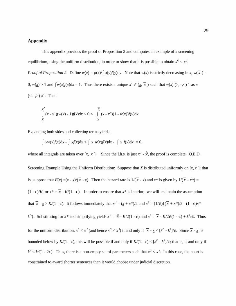
This appendix provides the proof of Proposition 2 and computes an example of a screening

equilibrium, using the uniform distribution, in order to show that it is possible to obtain xG < x J.

Proof of Proposition 2. Define w(x) = D(x)/ID(y)f(y)dy. Note that w(x) is strictly decreasing in x, w( xGG ) =

0, w(x) > 1 and Iw(x)f(x)dx = 1. Thus there exists a unique xN 0 (x, xGG ) such that w(x) (>,=,<) 1 as x

(<,=,>) xN. Then

xN xGGI (x - xN)(w(x) - 1)f(x)dx < 0 < I (x - xN)(1 - w(x))f(x)dx.x xN

Expanding both sides and collecting terms yields:

I xw(x)f(x)dx - I xf(x)dx < I xNw(x)f(x)dx - I xNf(x)dx = 0,

where all integrals are taken over [x, xGG ]. Since the l.h.s. is just x J - x̂ , the proof is complete. Q.E.D.

Screening Example Using the Uniform Distribution: Suppose that X is distributed uniformly on [x, xGG ]; that

is, suppose that F(x) =(x - x)/( xGG - x). Then the hazard rate is 1/( xGG - x) and x* is given by 1/( xGG - x*) =

(1 - ,)/K, or x* = xGG - K/(1 - ,). In order to ensure that x* is interior, we will maintain the assumption

that xGG - x > K/(1 - ,). It follows immediately that x J = (x + x*)/2 and xB = (1/,){( xGG + x*)/2 - (1 - ,)x*-

kD}. Substituting for x* and simplifying yields x J = x̂ - K/2(1 - ,) and xB = xGG - K/2,(1 - ,) + kP/,. Thus

for the uniform distribution, xB < x J (and hence xG < x J) if and only if xGG - x < [kD - kP]/,. Since xGG - x is

bounded below by K/(1 - ,), this will be possible if and only if K/(1 - ,) < [kD - kP]/,; that is, if and only if

kP < kD(1 - 2,). Thus, there is a non-empty set of parameters such that xG < x J. In this case, the court is

constrained to award shorter sentences than it would choose under judicial discretion.

30

References

Alexander, C.R., Arlen, J. and Cohen, M.A. “Regulating Corporate Criminal Sanctions: FederalGuidelines and the Sentencing of Public Firms.” Journal of Law and Economics, Vol. 42 (1999), pp. 393-422.

Ashenfelter, O., Eisenberg, T., and Schwab, S.J. “Politics and the Judiciary: The Influence of JudicialBackground on Case Outcomes.” Journal of Legal Studies, Vol. 24 (1995), pp. 257-281.

Banks, J.S. and Sobel, J. “Equilibrium Selection in Signaling Games.” Econometrica, Vol. 55 (1987), pp.647-662.

Besanko, D. and Spulber, D.F. “Contested Mergers and Equilibrium Antitrust Policy.” Journal of Law,Economics and Organization, Vol. 9 (1993), pp. 1-29.

Biskupic, J. and Flaherty, M.P. “Sentencing By the Book.” The Washington Post National WeeklyEdition, Vol. 13, No. 52 (1996), pp. 8-9.

Cho, I.K. and Kreps, D.M. “Signaling Games and Stable Equilibria.” Quarterly Journal of Economics,Vol. 102 (1987), pp. 179-221.

Cohen, M.A. “Explaining Judicial Behavior or What’s ‘Unconstitutional’ About the SentencingCommission?” Journal of Law, Economics and Organization, Vol. 7 (1991), pp. 183-199.

-------. “The Motives of Judges: Empirical Evidence from Antitrust Sentencing.” International Review ofLaw and Economics, Vol. 12 (1992), pp. 13-30.

Daughety, A.F. and Reinganum, J.F. “Keeping Society in the Dark: On the Admissibility of PretrialNegotiations as Evidence in Court.” RAND Journal of Economics, Vol. 26 (1995), pp. 203-221.

Freed, D.J. “Federal Sentencing in the Wake of Guidelines: Unacceptable Limits on the Discretion ofSentencers.” The Yale Law Journal, Vol. 101 (1992), pp. 1681-1754.

Grossman, G.M. and Katz, M.L. “Plea Bargaining and Social Welfare.” American Economic Review,Vol. 73 (1983), pp. 749-757.

Higgins, R.S. and Rubin, P.H. “Judicial Discretion.” Journal of Legal Studies, Vol. 9 (1980), pp. 129-138.

Miceli, T.J. “Plea Bargaining and Deterrence: An Institutional Approach.” European Journal of Lawand Economics, Vol. 3 (1996), pp. 249-264.

------- and Cosgel, M.M. “Reputation and Judicial Decision-Making.” Journal of Economic Behavior andOrganization, Vol. 23 (1994), pp. 31-51.

Meuller, C.B. and Kirkpatrick, L.C. 1996 Federal Rules of Evidence. New York: Little, Brown andCompany, 1996.

31

Nagel, I.H. and Schulhofer, S.J. “A Tale of Three Cities: An Empirical Study of Charging and BargainingPractices Under the Federal Sentencing Guidelines.” Southern California Law Review, Vol. 66 (1992), pp.501-566.

------- and -------. “Plea Negotiations Under the Federal Sentencing Guidelines: Guideline Circumventionand Its Dynamics in the Post-Mistretta Period.” Northwestern University Law Review, Vol. 91 (1997), pp.1284-1316.

O’Hara, E. “Social Constraint or Implicit Collusion? Toward a Game Theoretic Analysis of StareDecisis.” Seton Hall Law Review, Vol. 24 (1993), pp. 736-778.

Parker, J.S., and Block, M.K. “The Sentencing Commission, P.M. (Post-Mistretta): Sunshine or Sunset?”American Criminal Law Review, Vol. 27 (1989), pp. 231-288.

Posner, R.A.. “What Do Judges and Justices Maximize? (The Same Thing Everybody Else Does).”Supreme Court Economic Review, Vol. 3 (1993), pp. 1-42.

Rasmusen, E. “Judicial Legitimacy as a Repeated Game.” Journal of Law, Economics and Organization,Vol. 10 (1994), pp. 63-83.

Reinganum, J.F “Plea Bargaining and Prosecutorial Discretion.” American Economic Review, Vol. 78(1988), pp. 713-728.

------- and Wilde, L.L. “Settlement, Litigation and the Allocation of Litigation Costs.” RAND Journal ofEconomics, Vol. 17 (1986), pp. 557-566.

Rogoff, K. “The Optimal Degree of Commitment to an Intermediate Monetary Target.” QuarterlyJournal of Economics, Vol. 100 (1985), pp. 1169-1189.

Rubin, P.H. and Schrag, J.L. “Judicial Hierarchies and the Rule-Individual Tradeoff.” Working Paper,Emory University, 1996.

Spulber, D.F. and Besanko, D. “Delegation, Commitment, and the Regulatory Mandate.” Journal of Law,Economics and Organization, Vol. 8 (1992), pp. 126-154.

United States Sentencing Commission. The Federal Sentencing Guidelines: A Report on the Operationof the Guidelines System and Short-Term Impacts on Disparity in Sentencing, Use of Incarceration, andProsecutorial Discretion and Plea Bargaining, Executive Summary, Volume I and Volume II, 1991.

-------. 1995 Annual Report, 1995a.

-------. Guidelines Manual, 1995b.

32

Footnotes

1. Related analyses include Rogoff (1985), Spulber and Besanko (1992), and Besanko and Spulber

(1993), who show (respectively) that a president may prefer to appoint a more conservative central banker,

or a more activist regulatory agency head. Federal judges have life tenure and are intentionally insulated

from outside influences; changing their tastes may be more difficult than restricting their discretion.

2. In the federal guidelines, the maximum sentence cannot exceed the minimum by more than 25% or six

months, whichever is greater. Twenty-two states also have sentencing guidelines, though they typically

involve more judicial discretion and less prison time than for similar federal crimes (Biskupic and Flaherty,

1996, p.9).

3. According to Freed (1992, p. 1690), there are approximately 100 federal mandatory minimum penalties

contained in 60 different criminal statutes. Many of these involve drugs and/or the use of a gun.

4. In 1991, the Federal Sentencing Guidelines Governing Organizations were implemented to deal with

corporations convicted of a federal crime. Alexander, Arlen and Cohen (1999) find that total sanctions

increased as a consequence of these guidelines.

5. USSC Figure D (1995a, p. 52) reports an increase in the plea rate from 1991 to 1995. They (1995a, p.

51) attribute this to a composition effect, whereby the mix of offenses included more with typically low

trial rates (e.g., immigration) and fewer with typically high trial rates (e.g., drug trafficking).

33

6. It is not a pure charge offense system; “relevant conduct” (e.g., the amount of money in a fraud case,

the type and amount of drugs, or the use of a gun) can be considered in determining the applicable

sentencing range, independent of whether it was charged and proved.

7. A model examining prosecutorial discretion is developed in Reinganum (1988). Studies of post-

guidelines practice among prosecutors, focusing on guideline circumvention, have been conducted by Nagel

and Schulhofer (1992, 1997). They find that sentence bargaining has been largely replaced by bargaining

over the charge or guideline factors (mitigating or aggravating circumstances).

8. There is a voluminous literature on judicial objectives; for example, Ashenfelter, Eisenberg and Schwab

(1995) (political ideology); Cohen (1991, 1992) and Higgins and Rubin (1980) (potential for promotion);

Miceli and Cosgel (1994), O’Hara (1993) and Rasmusen (1994) (reputation); and Posner (1993) (all of the

above). Objectives of federal judges, who have life tenure, are particularly difficult to pin down.

9. Rubin and Schrag (1996) find that, even if appeals court and trial court judges have the same

preferences about enforcing a single contract, they make different decisions due to their different places in

the hierarchy because appeals court decisions affect more people, whose interests must also be considered.

10. Although the court can infer that negotiations failed if a case comes to trial, the details of plea

negotiations (what was offered, and any incriminating statements made during the failed negotiations) are

inadmissible as evidence under Federal Rule of Evidence 410 (Mueller and Kirkpatrick, 1996, p. 93).

11. As noted above, the court must verify that the sentence involved in the plea agreement falls within the

guidelines for the crime as charged, but the prosecutor determines the charge and is thereby able to make an

34

effective commitment to the ultimate sentence.

12. Miceli (1996) provides a model in which a legislature sets penalties to maximize deterrence,

anticipating that plea bargaining may dilute the deterrence effect. In my paper, both the sentencing

commission and the court maximize case-by-case justice, while the prosecutor pursues more prosaic

objectives.

13. This model of the court receiving an imperfectly informative public signal was introduced in Daughety

and Reinganum (1995) to examine the desirability of making currently inadmissible plea negotiations

admissible as evidence. When the public signal is uninformative, the court relies on all admissible evidence

in order to make a decision.

14. If there were a noisy (rather than completely uninformative) signal of x at trial, or if , were a function

of x, then D’s private information would bear on additional aspects of the problem besides the sentence

following an informative signal; both modifications complicate the existence of a revealing equilibrium.

15. In general, beliefs are a cumulative distribution function over the set of defendant types who would use

the strategy S with positive probability. Since we will always be dealing with revealing equilibria in this

stage, we can restrict attention to point beliefs, in which each such set is a singleton.

16. An alternative “reputation” model might assume that a judge trades off the disutility from imposing a

harsher sentence in one case for improved future plea outcomes. If plea bargaining depends on the average

(over all the judges) trial sentence, then harsher sentences are a public good which won’t be provided. I

thank Tracy Lewis and Preston McAfee for this observation.

35

17. For a proof of uniqueness, see Reinganum and Wilde (1986). When a revealing equilibrium exists,

equilibrium refinements may be invoked to eliminate pooling or partial pooling equilibria; either D1 (Cho

and Kreps, 1987) or universal divinity (Banks and Sobel, 1987) will do the trick in this case.

18. It is now easy to verify that S*(x; xT) = (1 - ,)x + ,xT - kP does minimize A D(S, x; r*(S; xT)). The

first-order condition is satisfied by construction and the second-order condition M2A D(S, x; r*(S; xT))/MS2 >

0 reduces to (2/K)exp{-( SGG - S)/K} - (1/K)exp{-( SGG - S)/K} > 0, which is clearly true.

19. One way to determine this posterior distribution is through updating the prior via the equilibrium

probability of trial. However, this posterior is also the actual frequency distribution of the public signal

which the court observes, since 1 - , of the time the public signal is informative.

20. I thank Daniel Kessler for suggesting this robustness check.

21. If plea bargaining did not exist, then ESL(xT) = (1 - ")ESET(xT) and xG = x J.

22. Grossman and Katz (1983) provide a screening model of plea bargaining in which the prosecutor’s

offer sorts guilty and innocent defendants.