Sensors fault detection architecture in a strongly ... · This paper’s objectives are to present...

22nd ITS World Congress, Bordeaux, France, 5–9 October 2015

ITS-2675

Sensors fault detection architecture in a strongly uncertain

environment

Nicolas Pous1, Dominique Gruyer2, Denis Gingras1

1. LIV, Sherbrooke University, Canada, [email protected], [email protected]

2. IFSTTAR- IM – LIVIC, Versailles-Satory, France, [email protected]

Abstract: Most of the solutions proposed in fault detection focusing on one part of the analyzed

system (Actuators, System, Sensors) supposing other parts in a nominal and well known state. In this

paper a new method aiming to complete a sensor fault detection without any assumptions made on the

comportment of the rest of the complete system is proposed. For that, a faults identification will be

proposed in order to reject defaults due to environmental perturbations or failure in the system or the

actuators, as we focus in this paper on sensor fault detection.

Keywords: Fault detection and identification, intelligent vehicle, Localization.

I Introduction

Autonomous or partially automatized vehicles need a perfect knowledge of their environment and

attitude, especially about their ego localization to operate safely. To ensure that, the use of GPS

receiver is necessary, however if we wish to refine the position estimation without having to use more

accurate, but also more expensive GPS receiver (RTK-GPS, DGPS), it’s possible to combine classical

GPS data with proprioceptive (Odometers, INS…) and exteroceptive (Lidar, Radar, etc.) sensors using

data fusion algorithms to provide a more precise position estimation [1-3]. Cooperative approach has

also been studied to improve the estimation result [4-5].

However, the use of data fusion algorithms suffers from reliability issues. Indeed, those algorithms are

sensitive to sensor failure as only one failure can lead to a significant error on the position estimation.

Since error sources increase by the number of used sensors in the system, the need for a fault detection

and identification scheme in order to quickly detect and isolate the corrupted information from the

faulty source is inevitable.

In contrast to frequently used model based methods [6], we propose a new FDI (Fault Detector and

Identification) architecture which doesn’t need a perfect knowledge of the system behaviour. Others

solutions deal with the non-linearity of the system [7]. But, considering both its important

non-linearity and the significant interaction with the environment (road condition, weather, etc.) the

mailto:[email protected]



Sensors fault detection architecture in a strongly uncertain environment

2

system behaviour study cannot be taken as a reference for fault detection.

Moreover, previously published methods generally assume that, in order to make a proper sensor fault

detection, all the other parts of the system are presenting a nominal behaviour [8]. However system

failure (Engine issues, flat tire, etc.) can also, just as the environmental interaction, impact the

measurement and be registered by the sensors. Identifying the failure source may be tricky.

This paper’s objectives are to present a sensor fault detection and identification architecture which

permit distinction between sensors faults and faults due to other sources. The proposed architecture is

inspired by multi-model data fusion algorithm as found in [9] that uses fuzzy decision laws with

analytic information redundancy to realize the detection of sensors faults. It consists in finding the

current vehicle dynamic mode by computing weights which correspond to the membership degree of a

given vehicle dynamic mode regarding the information coming from each sensor independently. Then,

a comparison between each weight and a mean value weight calculated instantaneously for all sensors

allow to observe behaviour divergence.

In order to insure the distinction between error sources (sensors/system/environmental, etc.), a three

dimensional analysis of the vehicle behaviour is also performed.

This paper is structured as follows: the second section will present the fault detector architecture and

the primary idea. In the third part, the three dimensional vehicle behaviour will be analysed in order to

help for the fault source discrimination. Some simulations results will be presented in section four,

with a first part concerning the study of detection algorithm and next simulation about the error source

distinction. We conclude this paper in the fifth section.

II fault detector algorithm

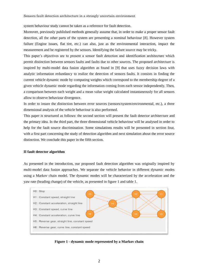
As presented in the introduction, our proposed fault detection algorithm was originally inspired by

multi-model data fusion approaches. We separate the vehicle behavior in different dynamic modes

using a Markov chain model. The dynamic modes will be characterized by the acceleration and the

yaw rate (heading change) of the vehicle, as presented in figure 1 and table 1.

Figure 1 - dynamic mode represented by a Markov chain


3

STRAIGHT

LINE

CURVE

CONSTANT SPEED H1 H3

SPEED CHANGE H2 H4

Table 1 – Dynamic modes definition

The Markov chain is designed to constrain the dynamic modes evolution according to Newtonian laws (we

can go from reverse gear to forward without stopping the vehicle for example), However in this paper we

focus on the four principle dynamic modes, H1 to H4 as described in Table1.

According to the description of the vehicle dynamic modes, we need both the angular speed and the linear

acceleration of the vehicle to determine the current dynamic mode. We will so determine these values with

the information of the proprioceptive sensors embedded in the vehicle.

Concerning the INS, these two values will be directly given by the sensor. For the odometer, it is necessary

to calculate (derivatives) these values since this sensor provides displacement and wheel angular speed data

only. We first compute the vehicle mean speed as follow,

_ ( ) _ ( )_ ( )

2

RW S t LW S tVe S t

(1)

where RW_S and LW_S are the right and left wheel speeds respectively. The acceleration value can be

obtained by computing the derivation of the previous equation.

( _ ) _ ( ) _ ( 1)( )

Odo

D VE S VE S t VE S tAcc t

Dt T

(2)

Concerning the angular speed of the vehicle, it’s possible to deduce it by computing the differential speed

from the two wheel speeds,

_ ( ) _ ( ) _ ( )Odo

Dif S t RW S t LW S t (3)

On the other hand, the compass, can provide us with heading and angular speed only, the latter being

computed by derivation of the heading θ(t).

( )_ ( )

Compass

tAn Sp t

t

(4)

These equations allow us to determine the two metrics used for the determination of the current vehicle

dynamic mode. As not all the sensors can provide information on the two of them (for example, compass,

not studied here, will only give information about orientation), the fault detection will be based on them

independently, which means that the metrics will be analyzed separately, in order to determine the presence

of an acceleration/rotation.

The presence of an acceleration and a rotation will respectively be represented by the variable Acc and Vθ.


4

Hence the four dynamic modes can be characterized by the four following equations.

1

2

3

4

H Acc V

H Acc V

H Acc V

H Acc V

(5)

Instead of performing a standard multi-hypothesis test giving a binary output value for each hypothesis by,

comparing the sensor data to a fixed threshold, we will instead compute for each hypothesis a weighted

value corresponding to a function of the membership degree of its acceleration and its rotation. This is

realized as described in figure 2, using a Gaussian membership function to determine the weight.

Figure 2 - weight determination using a Gaussian threshold

The weight is calculated as follow (example for the INS linear acceleration), with the σ coefficient value

allowing to adjust the sensitivity of the detector.

20.5*( / )

0.511 *

(0.4 * (2 * )INSA c

Acc

cexpP

pi

(6)

The complete fault detection architecture is presented in figure 3. The global hypothesis weight

computation is the instantaneous mean value of the weight for each metric (linear acceleration and yaw

rate) independently taking into account the weight from every sensor. It is calculated for the Acc weight

value in (7).


5

Figure 1 - Fault detection architecture

1 2

1

1

1( , ... ) ( )

N

N jN jj

i

i

Po Acc S S S C Po Acc S

C

(7)

Here, 1 2

( , ... )N

Po Acc S S S and ( )j

Po Acc S are respectively the mean weight for every sensor concerning

the acceleration and weight for the sensor j, and Cj is the corresponding decision. This decision is

represented in the fault detection architecture by the switch before the mean calculation step, which will be

controlled by the fault detection algorithm itself. It consists in the rejection of a faulty sensor in the mean

ponderation value determination.

The fault detection algorithm will process the residual generated from each sensor, by subtracting its own

weight value to the mean residual value coming from all sensors, as described in equation (8).

1 2( , ) ( , ... ) ( )

i N iR Acc S Po Acc S S S Po Acc S (8)

Assuming that a faulty sensor, uncorrelated with the other sensors output, introduces a perturbation ΔPo

in the weight computation, the residual of a faulty and a non-faulty sensors will then be affected as

described by equations (9) and (10), where ( )F

Po Acc S and ( )NF

Po Acc S are a faulty and a non-faulty

sensor weight respectively.

1 2

1 2

( ) ( ) ( , ... )

( ) ( ) ( , ... )

F F N

F NF N

R Acc S Po Acc S Po Acc S S S

R Acc S Po Acc S Po Po Acc S S S

(9)

1

1 1( ) ( ) ( )

N

NF NF i

i

R Acc S Po Po Acc S Po Acc SN N

(10)

According to these equations, we can determine the impact of a perturbation on the residual before the

decision ( (1 ) 1i

C i N ).

1F

NR Po

N

(11)

1NF

R PoN

(12)

Once a decision is made and the faulty source is discarded in the mean weight computation, a non-faulty


6

residual will correspond to a zero-mean process and the faulty one will present a perturbation bias equals to

the perturbation on the weight, ΔPo. This behavior will be investigated and illustrated with simulations in

section IV.

III Three dimensional behavior analysis

In the introduction, the problem of strong interactions with the environment was discussed. Indeed it

appears that a faulty behavior may arise from environmental perturbations, such as deteriorated roads or

climate changes, but also from other vehicular malfunctions, like a flat tire for example, which will affect

the vehicle dynamic states. As these perturbations will impact the residuals behavior, a three dimensional

analysis of the vehicle dynamic will help in the fault detection and identification process.

At first, we analyze the nominal 3D comportment for each of the four principle dynamic modes (H1 to H4).

As we know the longitudinal acceleration and the yaw rate defined around the Z-axe (figure 4), constitute

the two metrics for the determination of the vehicle dynamic mode.

Figure 2: Vehicle centered coordinate system

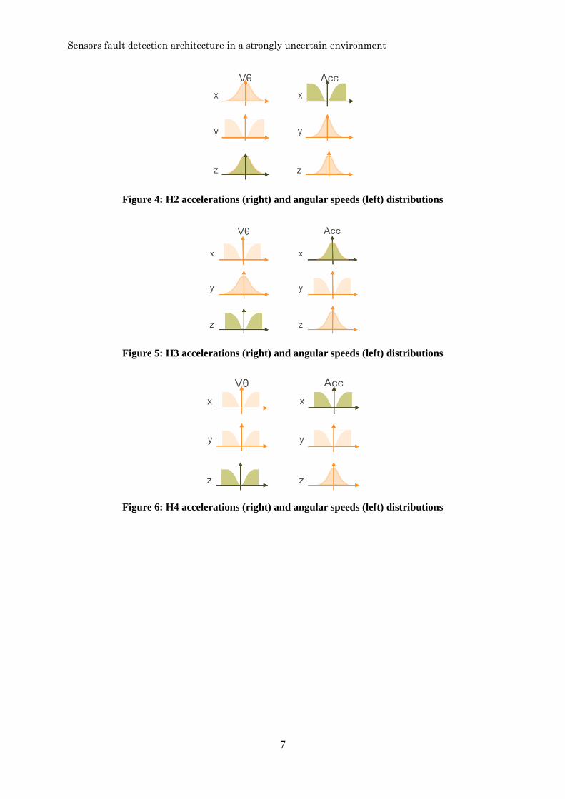
In the following representations (figure 5 to 8), it is possible to observe the theoretical distribution of both

acceleration and angular speed for each dynamic mode which can be registered during a scenario. Green

distributions are representing the longitudinal acceleration and the Z-axe angular speed, which result of

driver maneuvers (acceleration or direction change), will define the different dynamic modes. The others

non-zero centered distributions are due to the different forces applied to the vehicle during the driving, as

described in [10].

Figure 3: H1 accelerations (right) and angular speeds (left) distributions


7





8

Figure 7: Angular speed and acceleration distribution for the H4 dynamic mode

To verify these behaviors, Simulations have been run using the vehicle simulator ProSivic (software from

Civitec, France), which permit to simulate the dynamic behavior of a vehicle, and the output data generated

by the sensors. As it is possible to adjust speed and direction during the simulation, we built a scenario

which involves all the four dynamic modes considered in this study. All the dynamic modes have been

tested and their behavior validated correspond to the theoretical distributions we use as model. The H4

dynamic mode is presented here in Figure 9 to illustrate the simulation results.

It can be observed in the figure that the angular speed on the X and Y axis alone are not sufficient to be

relevant (they remain zero-centered even with a longitudinal acceleration), and the acceleration on the

Z-axis is centered on the gravity value (9.82 m/s2) instead of 0, but this component is present on every

simulation.

Once the vehicle behavior has been validated for every dynamic mode, it is now possible to use these

information in the fault identification algorithm.

IV Simulations

A- Sensor fault detection algorithm

In this section, we will examine the fault detection algorithm performance, assuming that the vehicle

present a normal behavior. Once again, we use the ProSivic Simulator software from Civitec to realize the

simulation.

To simulate a sensor failure, 100 seconds after the beginning of the simulation, a gain is injected on the

front left wheel speed measurement, which physically correspond to a tick lost on the corresponding

odometer. The figure 10 shows the residual behavior with the moment of the failure introduction marked by

a red line. The graphs are respectively representing INS, front and back odometers residuals. The failure

introduction increases the residuals variations for, and it also appears that the faulty sensor will present a


9

residual opposite to others and about twice their values (equations (11) and (12)).

It remains difficult to ensure a detection when the vehicle behavior presents strong accelerations or

direction changes. Indeed, each faulty behavior will affect differently the dynamic mode determination

(appearance of a dynamic change, missed detection of an event…). For example, the appearance of a sensor

failure may induce the detection of a vehicle rotation even if the real dynamic is descripting a straight line.

But if the vehicle remains in a rotation, the detection cannot be done.

Figure 10: Comportment of residuals with the introduction of a faulty behavior on one of the

sensors (front odometer)

A better way to ensure the occurrence of each dynamic mode is to analyze the mean values of all the

residual during a long time period involving the occurrence of all the dynamic mode in order to realize the

detection. The decision process is also add to the detection algorithm to reduce non-faulty residuals around

zero and increase the faulty residual value. The mean value is so calculated for 1000 samples, and the result

is presented in figure 11.

Figure 8: Residual mean value taking into account the decision procedure


10

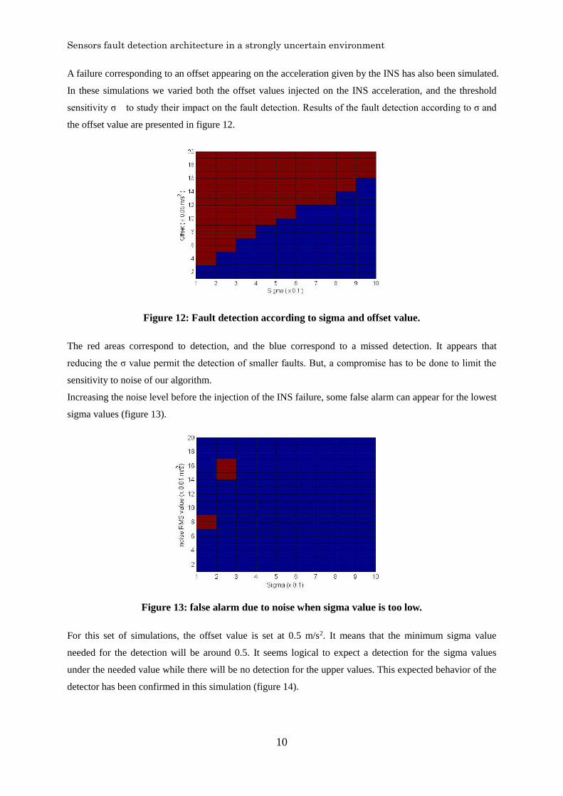
A failure corresponding to an offset appearing on the acceleration given by the INS has also been simulated.

In these simulations we varied both the offset values injected on the INS acceleration, and the threshold

sensitivity σ to study their impact on the fault detection. Results of the fault detection according to σ and

the offset value are presented in figure 12.

Figure 12: Fault detection according to sigma and offset value.

The red areas correspond to detection, and the blue correspond to a missed detection. It appears that

reducing the σ value permit the detection of smaller faults. But, a compromise has to be done to limit the

sensitivity to noise of our algorithm.

Increasing the noise level before the injection of the INS failure, some false alarm can appear for the lowest

sigma values (figure 13).

Figure 13: false alarm due to noise when sigma value is too low.

For this set of simulations, the offset value is set at 0.5 m/s2. It means that the minimum sigma value

needed for the detection will be around 0.5. It seems logical to expect a detection for the sigma values

under the needed value while there will be no detection for the upper values. This expected behavior of the

detector has been confirmed in this simulation (figure 14).


11

Figure 14: Offset detection with different sigma values varying noise level

A compromise is necessary to make a detector as sensitive as possible without introducing false alarm

due to noise present at the sensor output. It could be interesting to use filters to reduce noise impact,

but this can mask some faults which are supposed to be detected. This will be part of future

investigations.

The proposed architecture is efficient for almost of kind of failure, assuming that the faulty signal

present a level higher than the programmed sensitivity. This study is still in progress to permit the

configuration of the smallest sensitivity possible.

B- Identification of other sources of failure

Except from sensors, faults can result from environmental perturbations, vehicle malfunctions or vehicle

states changes (process deviations). In order to simulate these sources of malfunctions, three simulations

have been realized with the same trajectory but varying some road/vehicle parameters to simulate concrete

faults cases, which can generate dynamic changes.

- The first simulation corresponds to a nominal behavior, it will be used as a reference, and it

will also be possible to add faults on the sensors data to simulate a sensor fault.

- In the second one, the track parameters have been modified to integrate some perturbations on

the road altitude, corresponding to degradations of the surface (holes, undulation…).

- The last simulation represents a flat tire, appearing during a lapse of time and disappearing

after that. This is realized by modifying the wheel radius and shock absorber parameters.

To illustrate the behavior of each case, let us first compare the longitudinal acceleration for the same

trajectory.


12

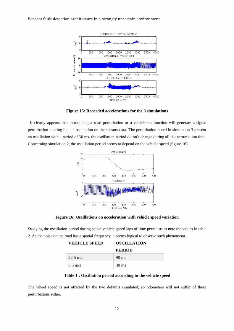
Figure 15: Recorded accelerations for the 3 simulations

It clearly appears that introducing a road perturbation or a vehicle malfunction will generate a signal

perturbation looking like an oscillation on the sensors data. The perturbation noted in simulation 3 present

an oscillation with a period of 30 ms. the oscillation period doesn’t change during all the perturbation time.

Concerning simulation 2, the oscillation period seems to depend on the vehicle speed (figure 16).

Figure 16: Oscillations on acceleration with vehicle speed variation

Studying the oscillation period during stable vehicle speed laps of time permit us to note the values in table

2. As the noise on the road has a spatial frequency, it seems logical to observe such phenomena.

VEHICLE SPEED OSCILLATION

PERIOD

22.5 m/s 90 ms

8.5 m/s 30 ms

Table 1 : Oscillation period according to the vehicle speed

The wheel speed is not affected by the two defaults simulated, so odometers will not suffer of these

perturbations either.


13

Observing the residual obtained for the acceleration (figure 17) it clearly appears that false alarm will be

generated if the detector consider the residual value only.

Figure 17: Residual value for the acceleration on three sensors (simulation2)

According to the description made in section III, the Z-acceleration is supposed to be zero centered with a

very low standard deviation for all the dynamic modes. Its simulated behavior is illustrated in Figure 18 for

the simulation 1 and 2. As the simulation behavior of scenario 3 during the appearance of the flat tire is

similar to the second simulation, we therefore focus on the results of the second simulation.

Figure 18: Z-Acceleration for the simulation 1 and 2

The two simulations exhibit a zero-mean acceleration, but the energy in the second case seems higher than

the first one. Computing the energy over 100 simulations has allowed us to analyze the difference.


14

Figure 19: Energy computed on 100 samples for the 2 simulations

The red curve representing the energy for the second simulation is always higher than the blue one (first

simulation).

Using this information, it is therefore possible to discriminate sensors failures from vehicle malfunctions or

road perturbations due to the environment or system parameters variation. But as the energy of the residuals

depends in theory on both the vehicle/environment perturbations and also on the dynamic mode considered

(the residual energy for the modes presenting an acceleration is higher), this aspect requires further

investigation but these results, showing two different energy levels is encouraging for the distinction

between sensors and environment faulty behaviors.

V Conclusion

This paper present the FDI architecture permitting to detect proprioceptive sensor failures. Using the three

dimensional comportment analysis, a discrimination between sensors faults and environmental

perturbations or system parameters variation has been developed too. The detection algorithm is tested in

section IV where two different fault cases are studied. The second case is also used to realize a short

performance analyze of the detection algorithm, depending on the detector characteristics and noise. The

discrimination process is then studied. Results allow us to observe differences between the behavior with

and without perturbation, which can lead to a good discrimination. This study will be continued to ensure

the sensor faults detection and identification, rejecting environmental or system perturbations. The

improvement of detector performances will also been pursued in further researches.

Acknowledgement

This work is part of CooPerCom, a 3-year international research project (Canada-France). The authors

would like to thank the National Science and Engineering Research Council (NSERC) of Canada and

the Agence nationale de la recherche (ANR) in France for supporting the project STP 397739-10.

This work is done in the LIV research group (Laboratory of Intelligent Vehicles), in the Electrical and


15

Computer Engineering Department of Sherbrooke University, (www.gel.usherbrooke.ca/LIV/public/),

Authors want to thank the LIV group members for their cooperation.

References

1. Cai Bai-gen ; Wang Jian ; Yin Qin ; Liu Jiang, (2009), A GNSS Based Slide and Slip Detection Method

for Train Positioning, Asia-Pacific Conference on Information Processing. APCIP 2009.

2. Kim, S.-B.; Bazin, J.-C.; Lee, H.-K.; Choi, K.-H.; Park, S.-Y. (2011), Ground vehicle navigation in harsh

urban conditions by integrating inertial navigation system, global positioning system, odometer and vision

data in Radar, Sonar & Navigation proceedings; Vol.5; pp 814 – 823.

3. Adrien Bak; Dominique Gruyer; Samia Bouchafa; Didier Aubert. (2012), Multi-Sensor Localization –

Visual Odometry as a Low Cost Proprioceptive Sensor; ITSC proceedings.

4. Rohani, M.; Gingras, D.; Vigneron, V.; Gruyer, D. (2013), A New Decentralized Bayesian Approach for

Cooperative Vehicle Localization based on fusion of GPS and Inter-vehicle Distance Measurements;

ICCVE.

5. M. Rohani; D. Gingras; D. Gruyer. (2014), Vehicular Cooperative Map Matching; International

Conference on Connected Vehicles and Expo (ICCVE).

6. Patton, R.J; Frank, P.; Clark, R. (1989) Fault Diagnosis in Dynamic Systems, Theory and Application;

prentice hall.

7. Mr. Huangqi Sun; Dr. M. Elizabeth Cannon. (1998), Reliability analysis of an ITS navigation system;

Department of Geomatics Engineering; The University of Calgary; Calgary, Alberta, Canada.

8. Patton, R.J.; Chen, J. (1991), Detection of faulty sensors in aero jet engine systems using robust

model-based methods, IEEE Colloquium on Condition Monitoring for Fault Diagnosis; pp 2/1 – 222.

9. Gruyer, D.; Pechberti, S.; Gingras, D.; Dupin, F. (2010), Robust positioning in safety applications for the

CVIS project; 2010 IEEE Intelligent Vehicles Symposium; pp 262 – 268

10. Sébastien Glaser. (2004), Modélisation et analyse d’un véhicule en trajectoires limites Application au

développement de systèmes d’aide à la conduite; PhD thesis; Université d'Evry.

http://www.gel.usherbrooke.ca/LIV/public/

Sensors fault detection architecture in a strongly ... · This paper’s objectives are to present...

Documents

Transcript of Sensors fault detection architecture in a strongly ... · This paper’s objectives are to present...