Sensorless Control of Permanent MagnetSynchronous Generators in Variable-Speed Wind

Turbine SystemsMohamed Abdelrahem

Student Member, IEEEInstitute for Electrical Drive Systems

and Power ElectronicsTechnische Universität München (TUM)

Munich, GermanyEmail: mohamed.abdelrahem@tum.de

Christoph HacklMember, IEEE

Munich School of Engineering Research Group“Control of Renewable Energy Systems (CRES)”

Technische Universität München (TUM)Munich, Germany

Email: christoph.hackl@tum.de

Zhenbin Zhang, Ralph KennelStudent Member, Senior Member, IEEE

Institute for Electrical Drive Systemsand Power Electronics

Technische Universität München (TUM)Munich, Germany

Email: james.cheung, ralph.kennel@tum.de

Abstract—This paper proposes a sensorless control strategy forpermanent magnet synchronous generators (PMSGs) in variable-speed wind turbine systems (WTSs). The proposed scheme usesan extended Kalman filter (EKF) for estimation of rotor speedand position. For EKF design, the nonlinear state space model ofthe PMSG is derived. Estimation and control performance of theproposed sensorless control method are illustrated by simulationresults for all operation conditions. Moreover, the performanceof the proposed EKF is tested under variations of the PMSGparameters.

NOTATION

N,R,C are the sets of natural, real and complex numbers.x ∈ R or x ∈ C is a real or complex scalar. x ∈ Rn (bold)is a real valued vector with n ∈ N. x> is the transpose and‖x‖ =

√x>x is the Euclidean norm of x. 0n = (0, . . . , 0)>

is the n-th dimensional zero vector. X ∈ Rn×m (capital bold)is a real valued matrix with n ∈ N rows and m ∈ N columns.O ∈ Rn×m is the zero matrix. xyz ∈ R2 is a space vector of astator (s) or filter (f ) quantity, i.e. z ∈ s, f. The space vectoris expressed in either phase abc-, stationary s-, or arbitrarilyrotating k-coordinate system, i.e. y ∈ abc, s, k, and mayrepresent voltage u, flux linkage ψ or current i, i.e. x ∈u,ψ, i. Ex or EX is the expectation value of x orX , respectively.

I. INTRODUCTION

The electrical power generation by renewable energysources (such as e.g. wind) has increased significantlyduring the last years contributing to the reduction of carbondioxide emissions and to a lower environmental pollution [1].This increase will continue as countries are extending theirrenewable action plans. Therefore, the share of wind powergeneration will increase further worldwide. Among variouswind energy conversion system (WECS) configurations, thedoubly-fed induction generator (DFIG)-based variable-speedWECSs have been the dominant technology in the marketsince late 1990s [1]-[3], see Fig 1. DFIGs can supplyactive and reactive power, operate with a partial-scale powerconverter (around 30% of the machine rating), and achieve a

certain ride through capability [3]. Operation above and belowthe synchronous speed is feasible. However, this situationhas changed in the recent years with the development ofWECSs with larger power capacity, lower cost/kW, increasedpower density, and the need for higher reliability. More andmore attention has been paid to direct-drive gearless WECSconcepts. Among different types of generators, the permanentmagnet synchronous generator (PMSG), see Fig 2, has beenfound to be superior owing to their advantages of higherefficiency, higher power density, lower maintenance cost,and better grid compatibility [1]. Increased reliability andhigh performance make direct-drive PMSG-based WECSsmore attractive in multi-Megawatt offshore applications,where the WECSs are installed in harsh and less-accessibleenvironments. Currently, there is a variety of commercialdirect-drive PMSG-based WECSs in the market with powerratings ranging from hundreds of watts to 6 MW [1].

DFIG

Grid

Wind

Turbine Back-back converter filter

Gear box

Figure 1: DFIG topology for variable-speed wind turbinesystems.

Vector control has – so far – proven to be the most popularcontrol technique for PMSGs in variable-speed WTSs [4]. Thismethod allows for a decoupled control of active and reactivepower of WTSs via regulating the direct and quadraturecomponents of the stator current vector independently. Vectorcontrol requires accurate knowledge of rotor speed and rotorposition [4]. Recently, the interest in sensorless methods (see,

PMSG

GridWind

TurbineBack-back converter filter

Figure 2: PMSG topology for variable-speed wind turbinesystems.

e.g., [5] and references therein) is increasing due to cost effec-tiveness/robustness, which implies that the vector controllersmust operate without the information of mechanical sensors(such as position encoders or speed transducers) mounted onthe shaft. The required rotor signals must be estimated via theinformation provided by electrical (e.g. current) sensors whichare cheap and easier to install than mechanical sensors. Fur-thermore, mechanical sensors reduce the system reliability dueto their high failure rate, which implies shorter maintenanceintervals and, so, higher costs [4]-[7].

Many position sensorless control schemes have beendeveloped for permanent magnet synchronous machines(PMSMs) used in applications such as electric vehicles, homeappliances, and industrial drives [5]. Although little work hasbeen reported on position sensorless vector control for PMSG-based WECSs, the methods developed for other industrialsensorless PMSM drives can be adapted to PMSG-basedWECS applications. Position sensorless vector control forPMSGs used in direct-drive WECSs could be easier than thosein other industrial applications because of several factors.First, the difference between the d- and q-axis inductancesof the PMSGs used in direct-drive WECSs is usually small(Ld ≈ Lq). Sensorless control of a nonsalient-pole PMSG ismuch easier than that of a PMSM with large saliency in themedium- and high-speed range. Second, the operation speedof PMSGs used in WECSs are relatively limited and rarelyreach the flux-weakening region.

Generally the rotor speed/position estimation schemesapplicable for PMSGs can be grouped into two categories: 1)open-loop calculation (such as flux-based method, inductancebased method, etc...) and 2) closed loop observers (suchas model reference adaptive system (MRAS), sliding modeobserver (SMO), etc..) [5]. The extended Kalman filter(EKF) is an optimal estimator in the least-square sense forestimating the states of dynamic nonlinear systems [8]. EKFhas already been used for sensorless control and estimationof the electrical parameters of AC machines [8]-[15].

In [13], an EKF was designed in the stationary referenceframe s = (α, β) for PMSG speed and position estimation.However, this paper neglected the mechanical system

dynamics as the author assumes dωdt = 0. A sensorless control

of distributed power generators based on derivative freeKalman filter has been proposed in [14]. For the proposedmethod, the generator model is first subject to a linearizationbased on differential flatness and next state estimation isperformed by applying the standard Kalman filter recursionto the linearized model. In [15], an EKF was designed inthe rotating reference frame k = (d, q) for PMSG speedand position estimation. However, this paper neglected themechanical system dynamics as the author also assumesdωdt = 0. Neglecting the mechanical system dynamics worsensthe estimation performance of the EKF (see results in [15])and will not represent the real physical model of the system.The observability of the linearized PMSG model is notchecked in all previous works [12]-[15].

In this paper, an extended Kalman filter is proposed for theestimation of speed and position of the PMSG rotor. State,input and measurement variables are used in the rotatingreference frame k = (d, q), which reduces the complexityof the state, input and measurement matrices and, hence, thecomputational time for real-time implementation. The EKFperformance and its robustness against parameter variationsare illustrated via simulation results. The results highlight theability of the EKF in tracking the PMSG rotor speed andposition.

II. MODELING AND CONTROL OF THE WTS WITH PMSGThe block diagram of the vector control problem of WTS

with PMSG is shown in Fig. 3. It consists of a permanentmagnet synchronous machine mechanically coupled to thewind turbine directly via a stiff shaft. The stator windingsof the PMSG are connected via a back-to-back full-scalevoltage source converter (VSC), a filter and a transformer tothe grid. The transformer will be neglected in the upcomingmodeling. The machine side converter (MSC) and the grid sideconverter (GSC) share a common DC-link with capacitanceCdc [As/V] with DC-link voltage udc [V]. Detailed models ofthese components can be found in [16]. The stator voltageequation of the PMSG is given by [16]:

uabcs (t) = Rsiabcs (t) +

d

dtψabcs (t), ψabcs (0) = 03 (1)

whered

dtψabcs (t) = Ls

d

dtiabcs (t) + eabcs (t) (2)

Here uabcs = (uas , ubs , u

cs )> [V], iabcs = (ias , i

bs , i

cs )> [A],

ψabcs = (ψas , ψbs, ψ

cs)> [Vs], and eabcs = (eas , e

bs, e

cs)> [V] are

the stator voltages, currents, fluxes, and back electromotiveforces respectively, all in the abc-reference frame (three-phasesystem). Rs [Ω] and Ls [Vs/A] are the stator resistance andinductance.Note that the PMSG rotor rotates with mechanical angularfrequency ωm [rad/s]. Hence, for a machine with pole pairnumber np [1], the electrical angular frequency of the rotor isgiven by

ωr = npωm

C

PI

abc/dqPLL

dq/a

bc

PW

M

Drive

PI

abc/dq

PI

MSC

PI

dq/a

bc

PW

M

Drive

PI

abc/dq

PI

GSC

DC

Link

Wind turbine

Grid

PMSG

Encoder

abc

siabc

su

dcC

dcu

abc

fi

abc

ou

d

refsi ,

d

siabc

si

q

si

q

ssr iL

)( pm

d

ssr iL r

refr ,q

refsi ,

q

ffe iL

d

ffe iL

dcurefdcu ,

abc

ou

abc

fi

q

reffi ,

q

fi

d

reffi ,

d

fi abc

oud

ou

q

ou

fL

fR

rr &

rr

e e

e

Figure 3: PMSG control structure for variable-speed wind turbine systems.

and the rotor reference frame is shifted by the rotor angle

φr(t) =

∫ t

0

ωr(τ)dτ + φ0r, φ0

r ∈ R (3)

with respect to the stator reference frame (φ0r is the initial

rotor angle). Equation (1) can be expressed in the stationaryreference frame as follows

xk = TP (φ)−1xs = TP (φ)−1 TCxabc︸ ︷︷ ︸

xs=(xα,xβ)>

by using the Clarke and Park transformation (see, e.g., [16]),respectively, given by (neglecting the zero sequence)

xs=γ

[1 − 1

2 − 12

0√

32 −

√3

2

]︸ ︷︷ ︸

=:TC

xabc & xk=

[cos(φ) sin(φ)− sin(φ) cos(φ)

]︸ ︷︷ ︸

=:TP (φ)−1

xs

(4)where γ = 2

3 for an amplitude-invariant transformation (orγ =

√2/3 for a power-invariant transformation). Therefore,

(1) can be rewritten in the stationary reference frame s =(α, β) as follows

uss (t) = Rsiss (t) +

d

dtψss (t), ψss (0) = 02 (5)

Equation (5) can be written in the rotating reference framek = (d, q) as

uks (t) = Rsiks (t)+

d

dtψks (t)+ωrJψ

ks (t), ψks (0) = 02 (6)

where [16]

J := TP (π/2) =

[0 −11 0

].

Assuming Lds = Lqs =: Ls (no anisotropy), the PMSG fluxcan be expressed by

ψks =

(ψdsψqs

)= Ls

(idsiqs

)+

(ψpm

0

)(7)

and the dynamics of the mechanicals of the (stiff) wind turbinesystem are given by

d

dtωm =

1

Θ

(me −mm

), ωm(0) = ω0

m ∈ R (8)

whereme =

3

2npψpmi

qs and mm =

ptωm

(9)

are the electro-magnetic machine torque (moment) and themechanical wind turbine torque, respectively. The mechani-cal torque mm depends on the wind turbine power pt [W](see Sec. III) and the mechanical angular speed ωm [rad/s].Θ [kg/m2] is the rotor inertia and np [1] is the pole pairnumber.

A. Overall nonlinear model of the PMSG

For the design of the EKF, the derivation of a compact(nonlinear) state space model of the PMSG of the form

d

dtx = g(x,u), x(0) = x0 ∈ R4 and y = h(x), (10)

is required. Therefore, introduce the state vector x, the output(measurement) vector y and the input vector u as follows

x =(ids iqs ωr φr

)> ∈ R4,

y =(ids iqs

)> ∈ R2,

u =(uds uqs

)> ∈ R2.

(11)

Inserting (7) into (6), solving for ddti

ks and inserting (9) into (8)

and solving for ddtωr yields the nonlinear model (17) with

g(x,u) =

−RsLs

ids + ωriqs + 1

Lsuds

−RsLs

iqs − ωrids − ωrLsψpm + 1

Lsuqs

npΘ

[32npψpmi

qs −mm]

ωr

(12)

andh(x) =

[1 0 0 00 1 0 0

]x. (13)

Note that it is assumed that the mechanical torque mm asin (9) is known (at least roughly using the wind power asin (14) and the power coefficient as in (16)).

B. Overall control system of the WTS

The complete control block diagram of the PMSG in fieldoriented control is depicted in Fig. 3. For the machine-sideconverter (MSC), the q-axis current is used to controlthe PMSG stator active power in order to harvest themaximally available wind power (i.e., maximum powerpoint tracking, see Sec. III), whereas the d-axis current isused to control the reactive power flow in the PMSG [4], [20].

For the grid-side converter (GSC), the stator voltage orienta-tion is used [4], [16], which allows for independent control ofactive (d-axis current) and reactive power (q-axis current) flowbetween grid and GSC. The main control objective of the GSCis to assure an (almost) constant DC-link voltage regardless ofmagnitude and direction of the power flow. DC-link voltage

control is a non-trivial task due to the possible non-minimum-phase behavior for a power flow from the grid to the DC-link [16], [17], [18]. More details on controller design, phase-locked loop or, alternatively, virtual flux estimation and pulse-width modulation (PWM) are given in, e.g., [4], [19], [16].

III. MAXIMUM POWER POINT TRACKING (MPPT)

Wind turbines convert wind energy into mechanical energyand, via a generator, into electrical energy. The mechanical(turbine) power of a WTS is given by [20], [16], [21]:

pt = cp(λ, β)1

2ρπr2

t v3w︸ ︷︷ ︸

wind power

(14)

where ρ > 0 [kg/m3] is the air density, rt > 0 [m] is theradius of the wind turbine rotor (πr2

t is the area swept by theturbine), cp ≥ 0 [1] is the power coefficient, and vw ≥ 0 [m/s]is the wind speed. The power coefficient cp is a measure forthe “efficiency” of the WTS. It is a nonlinear function of thetip speed ratio

λ =ωmrtvw

≥ 0 [1] (15)

and the pitch angle β ≥ 0 [] of the rotor blades. The Betz limitcp,Betz = 16/27 ≈ 0.59 is an upper (theoretical) limit of thepower coefficient, i.e. cp(λ, β) ≤ cp,Betz for all (λ, β) ∈ R×R.For typical WTS, the power coefficient ranges from 0.4 to 0.48[20], [21]. Many different (data-fitted) approximations for cphave been reported in the literature. This paper uses the powercoefficient from [21], i.e.

cp(λ, β) = 0.5176

(116

λi− 0.4β − 5

)e−21λi + 0.0068λ

1

λi:=

1

λ+ 0.08β− 0.035

β3 + 1. (16)

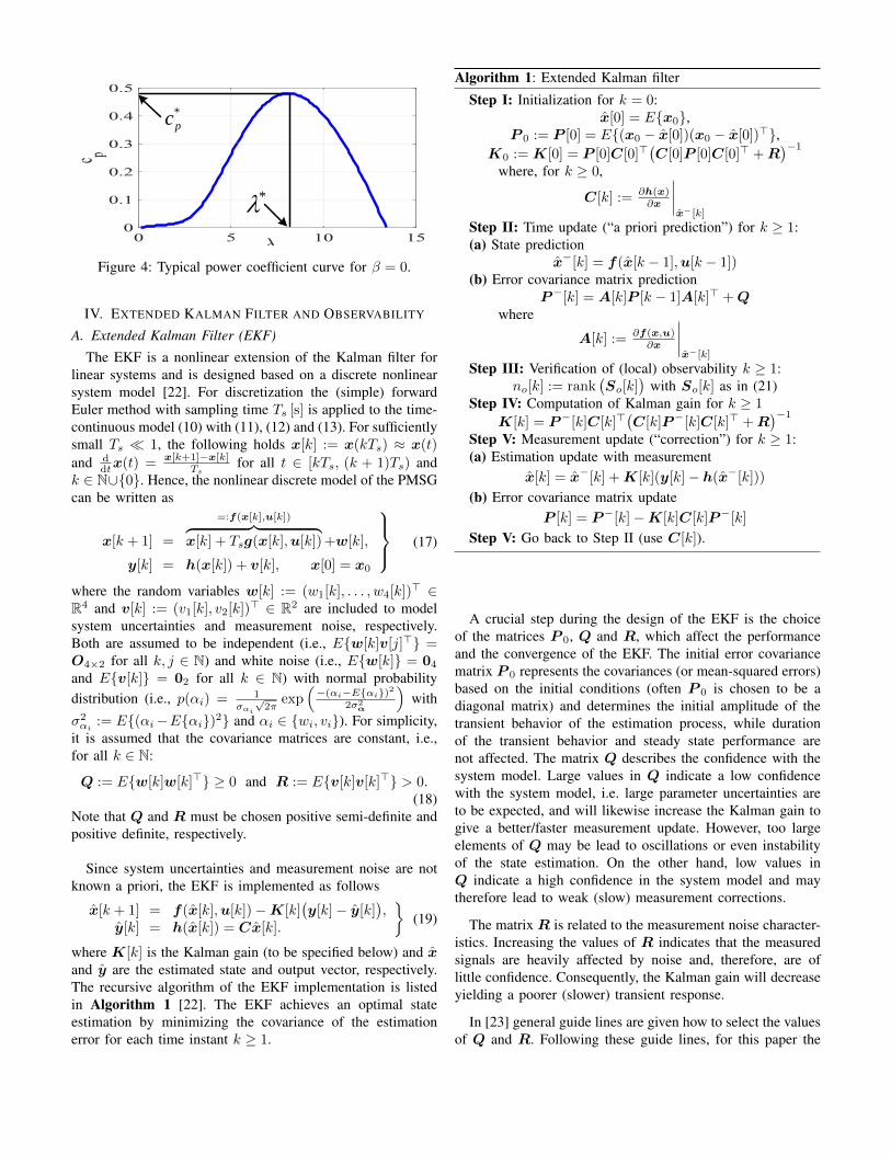
For wind speeds below the nominal wind speed of the WTS,maximum power tracking is the desired control objective.Here, the pitch angle is held constant at β = 0 and theWTS must operate at its optimal tip speed ratio λ? (a givenconstant) where the power coefficient has its maximum valuec?p := cp(λ

?, 0) = maxλ cp(λ, 0) as shown in Fig. 4. Onlythen, the WTS can extract the maximally available turbinepower p?t := c?p

12ρπr

2t v

3w [16].

Maximum power point tracking is achieved by a speedcontroller, Fig. 3, which assures that the generator angularfrequency ωm is adjusted to the actual wind speed vw such thatωmrtvw

!= λ? holds. Therefore, the optimum generator angular

frequency ωm,ref can be calculated and then it is comparedwith the actual mechanical speed ωm, which is estimatedby the EKF, as shown in Fig. 3. Based on the differenceωm,ref −ωm the underlying PI controller generates the q-axisstator reference current iqs,ref .

*

pc

*

Figure 4: Typical power coefficient curve for β = 0.

IV. EXTENDED KALMAN FILTER AND OBSERVABILITY

A. Extended Kalman Filter (EKF)

The EKF is a nonlinear extension of the Kalman filter forlinear systems and is designed based on a discrete nonlinearsystem model [22]. For discretization the (simple) forwardEuler method with sampling time Ts [s] is applied to the time-continuous model (10) with (11), (12) and (13). For sufficientlysmall Ts 1, the following holds x[k] := x(kTs) ≈ x(t)

and ddtx(t) = x[k+1]−x[k]

Tsfor all t ∈ [kTs, (k + 1)Ts) and

k ∈ N∪0. Hence, the nonlinear discrete model of the PMSGcan be written as

x[k + 1] =

=:f(x[k],u[k])︷ ︸︸ ︷x[k] + Tsg(x[k],u[k]) +w[k],

y[k] = h(x[k]) + v[k], x[0] = x0

(17)

where the random variables w[k] := (w1[k], . . . , w4[k])> ∈R4 and v[k] := (v1[k], v2[k])> ∈ R2 are included to modelsystem uncertainties and measurement noise, respectively.Both are assumed to be independent (i.e., Ew[k]v[j]> =O4×2 for all k, j ∈ N) and white noise (i.e., Ew[k] = 04

and Ev[k] = 02 for all k ∈ N) with normal probabilitydistribution (i.e., p(αi) = 1

σαi√

2πexp

(−(αi−Eαi)2

2σ2α

)with

σ2αi := E(αi−Eαi)2 and αi ∈ wi, vi). For simplicity,

it is assumed that the covariance matrices are constant, i.e.,for all k ∈ N:

Q := Ew[k]w[k]> ≥ 0 and R := Ev[k]v[k]> > 0.(18)

Note that Q and R must be chosen positive semi-definite andpositive definite, respectively.

Since system uncertainties and measurement noise are notknown a priori, the EKF is implemented as follows

x[k + 1] = f(x[k],u[k])−K[k](y[k]− y[k]

),

y[k] = h(x[k]) = Cx[k].

(19)

where K[k] is the Kalman gain (to be specified below) and xand y are the estimated state and output vector, respectively.The recursive algorithm of the EKF implementation is listedin Algorithm 1 [22]. The EKF achieves an optimal stateestimation by minimizing the covariance of the estimationerror for each time instant k ≥ 1.

Algorithm 1: Extended Kalman filter

Step I: Initialization for k = 0:x[0] = Ex0,

P 0 := P [0] = E(x0 − x[0])(x0 − x[0])>,K0 := K[0] = P [0]C[0]>

(C[0]P [0]C[0]> +R

)−1

where, for k ≥ 0,

C[k] := ∂h(x)∂x

∣∣∣∣x−[k]

Step II: Time update (“a priori prediction”) for k ≥ 1:(a) State prediction

x−[k] = f(x[k − 1],u[k − 1])(b) Error covariance matrix prediction

P−[k] = A[k]P [k − 1]A[k]> +Qwhere

A[k] := ∂f(x,u)∂x

∣∣∣∣x−[k]

Step III: Verification of (local) observability k ≥ 1:no[k] := rank

(So[k]

)with So[k] as in (21)

Step IV: Computation of Kalman gain for k ≥ 1

K[k] = P−[k]C[k]>(C[k]P−[k]C[k]> +R

)−1

Step V: Measurement update (“correction”) for k ≥ 1:(a) Estimation update with measurement

x[k] = x−[k] +K[k](y[k]− h(x−[k]))

(b) Error covariance matrix updateP [k] = P−[k]−K[k]C[k]P−[k]

Step V: Go back to Step II (use C[k]).

A crucial step during the design of the EKF is the choiceof the matrices P 0, Q and R, which affect the performanceand the convergence of the EKF. The initial error covariancematrix P 0 represents the covariances (or mean-squared errors)based on the initial conditions (often P 0 is chosen to be adiagonal matrix) and determines the initial amplitude of thetransient behavior of the estimation process, while durationof the transient behavior and steady state performance arenot affected. The matrix Q describes the confidence with thesystem model. Large values in Q indicate a low confidencewith the system model, i.e. large parameter uncertainties areto be expected, and will likewise increase the Kalman gain togive a better/faster measurement update. However, too largeelements of Q may be lead to oscillations or even instabilityof the state estimation. On the other hand, low values inQ indicate a high confidence in the system model and maytherefore lead to weak (slow) measurement corrections.

The matrix R is related to the measurement noise character-istics. Increasing the values of R indicates that the measuredsignals are heavily affected by noise and, therefore, are oflittle confidence. Consequently, the Kalman gain will decreaseyielding a poorer (slower) transient response.

In [23] general guide lines are given how to select the valuesof Q and R. Following these guide lines, for this paper the

0

0.3

0.2

0.1time (sec)

r r][r

ad

r

05

10

152025

]/

[s

mv w

rr

0

0

100

200

300

400]/

[s

rad

r

2

4

6

8

0.4 0.6 0.80

2

4]1[

rank

0.2 0.4 0.5

time (sec)

Figure 5: Estimation performance of the proposed EKF (fromtop): wind speed vw, rotor speed ωr, Observability matrixrank, and rotor angle φr.

following values have been selected

Q = diag0.5, 0.5, 1 · 10−6, 5 · 10−3R = diag1, 1 (20)P 0 = diag1, 1, 0.001, 10x0 = (5, 0.1, 0, 0)>

B. Observability

The observability of a linear system can be verified bycomputing the observability matrix and its rank. For nonlinearsystems, it is possible to analyze the observability “locally”by analyzing the linearized model around an operating point[24]. The observability matrix of the linearized model of theconsidered PMSG as in (17) is given by

So[k] :=

C[k]

C[k]A[k]C[k]A[k]2

C[k]A[k]3

∈ R8×4, (21)

where A[k] and C[k] are computed numerically1 for eachsampling instant k ≥ 0 (see Algorithm 1). The pairA[k],C[k] (i.e., the linearized model of the PMSG) islocally observable if and only if the observability matrix So[k]has full rank, i.e., rank

(So[k]

)= 4 for the considered PMSG

as in (17). To check “local” observability, the rank of theobservability matrix So[k] is computed numerically for eachsampling instant k ≥ 0 in Step III of Algorithm 1.

1Future work will derive analytical conditions for local observability.

0 0.30.1time (sec)

r r][r

ad

r

05

10

152025

]/

[s

mv w

rr

0

0

100

200

300

400]/

[s

rad

r

2

4

6

8

0.2 0.4

0

0.1

0.2

0.3

0.4

][

sR

Figure 6: Estimation performance of the proposed EKF at 50%step change in the PMSG resistance Rs (from top): wind speedvw, PMSG stator resistance Rs, rotor speed ωr, and rotor angleφr.

V. SIMULATION RESULTS AND DISCUSSION

A simulation model of a 16 kW WTS with PMSG isimplemented in Matlab/Simulink. The system parametersare listed in Table I. The implementation is as in Fig. 3.For more details on the implementation of e.g. back-to-backconverter, PWM, current controller design, see [16]. Thesimulation results are shown in Figs. 5-9. The estimationperformances of EKF are compared with the actual values fordifferent wind speed and parameter uncertainties in Rs and Ls.

Fig. 5 shows the simulation results for variable windspeeds. The presented wind speeds cover almost the completespeed range of the PMSG-based WTS (from low to highspeed). Fig. 5 illustrates the tracking capability of the EKFof rotor speed and rotor position at low and high speeds. TheEKF shows a high estimation accuracy as the estimation erroris very small, see Table. II. The observability of the linearizedPMSG model has been tested online under variable windspeeds, see Fig. 5: The linearized system is observable evenif the PMSG operates at low speed, i.e., the stator frequencyis almost zero (as shown in Fig. 5). The observability matrixhas full rank for all times, i.e. rank

(So[k]

)= 4 for all k ≥ 0.

In order to check the robustness of the EKF under(unknown) parameter variations of the PMSG, the valueof the stator resistance Rs is increased by 50% (e.g. dueto warming or aging). For this scenario, Fig. 6 shows theestimation performances of the proposed EKF. The simulatedwind speed profile is depicted in Fig. 6 (top). It is clear that

the EKF is robust against parameter uncertainties in Rs.It estimates rotor speed and rotor position with very smallerrors (see Tab. II).

0 0.30.1time (sec)

r r][r

ad

r

05

10

152025

]/

[s

mv w

rr

0

0

100

200

300

400]/

[s

rad

r

2

4

6

8

0.2 0.4

8

12

16

20

][m

HL

s

Figure 7: Estimation performance of the proposed EKF at 25%step change in the PMSG inductance Ls (from top): windspeed vw, PMSG inductance Ls, rotor speed ωr, and rotorangle φr.

Table I: Parameters of the PMSG-based WTS.

Name Nomenclature ValueWind turbine rated power pt 16 kWWind turbine radius rt 1.6 mRated wind speed vwrated 20 m/secOptimal tip speed ration λ? 8.11PMSG rated power pnom 16 kWPMSG rated voltage (line-line] urms

s 400 VNumber of pair poles np 3Stator resistance Rs 0.2[Ω]Stator inductance Ls 15 mHPermanent magnet flux ψpm 0.85PMSG moment of inertia Θ 0.02[kg/m2]DC capacitor Cdc 3[mF]DC-link voltage udc 700[V]Grid line-line voltage uo 400[V]Grid normal frequency fe 50[Hz]Grid resistance Rg 0.036[Ω]Grid inductance Lg 2[mH]Filter resistance Rf 0.12[Ω]Filter inductance Lf 8[mH]Sampling time Ts 40[µs]Simulation step Tsim 1[µs]

Table II: Estimation errors of the proposed EKF.

Simulation case ωr φr

Normal conditions 0.9% 1.2%Rs increased by 50% 1.15% 1.4%Ls increased by 25% 1.8% 2.6%

0.80.2

time [sec]

05

10

152025

]/

[s

mv w

0

8.1

300

600

900

1200][r

pm

m

0

20

][

&A

ii

q s

d s

0.4 1.0 1.2

40

60

80q

refsi ,

q

si d

refsi ,

d

si

8.2

8.0

]1[

0.48

0.47

0.49

]1[p

c

20

15

10

5

0

QkW

P&]

[P QmaxP

0.6 1.4

refm,m

Figure 8: Performance of the MSC control system (from top):wind speed vw, rotor mechanical speed ωm, d & q currents ids& iqs, tip speed ratio λ, power coefficient cp, and output activeand reactive power P & Q.

Finally, the robustness with respect to changes (dueto magnetic saturation) in the stator inductance Ls isinvestigated. Therefore, Ls is increased by 25%. Fig. 7 showsthe simulation results of the proposed EKF for this scenario.The used wind speed profile is depicted in Fig. 7 (top).Again, the EKF shows an accurate estimation performanceand robustness against parameter uncertainties (see Tab. II).

The final simulation results are shown in Fig. 8 and Fig. 9.Fig. 8 illustrates the control performance of the machine sideconverter under variable wind speed (top). It is clear thatthe MSC guarantees tracking of the maximum power fromthe wind turbine. The actual rotor speed wm of the PMSGis following the reference value wm,ref , which ensures theMPPT capability. The power coefficient cp(λ, 0) is kept closeto its maximal (optimal) value c?p ≈ 0.48 when the optimaltip speed ratio λ? ≈ 8.11 is reached. Moreover, the generatedpower from the PMSG is almost equal the maximum poweras shown in Fig. 8 (bottom). Also, the GSC control systemensures practical tracking of the constant reference DC

675

700

725]

[Vu

dc

dcu refdcu ,

0.80.2

time [sec]

0.4 1.0 1.20.6 1.4

d

reffi ,

d

fiq

reffi ,

q

fi

1020304050

0

][

&A

ii

q f

d f

Figure 9: Performance of the GSC control system (from top):DC-link voltage udc, and d & q currents idf & iqf .

voltage (with some small deviations) and of the references d& q currents as shown in Fig. 9.

VI. CONCLUSION

This paper proposed a sensorless vector control method forvariable-speed wind turbine systems (WTSs) with permanentmagnet synchronous generator (PMSG). The method uses anextended Kalman filter (EKF) for estimating the PMSG rotorspeed and position. For the design of the EKF, a nonlinearstate space model of the PMSG has been derived. The designprocedure of the EKF has been presented in detail. Thesensorless control scheme of the WTS with PMSG has beenillustrated by simulation results and its performance has beencompared with the real values of the rotor speed and position.The results have shown that the EKF tracks rotor speed andposition with high accuracy. Moreover, the EKF is robust tovariations in the PMSG stator resistance and inductance.

REFERENCES

[1] M. Liserre, R. Cardenas, M. Molinas, and J. Rodriguez, “Overviewof Multi-MW Wind Turbines and Wind Parks”, IEEE Transactions onIndustrial Electronics, Vol. 58, No. 4, pp. 1081–1095, April 2011.

[2] A. Hansen, F. Iov, F. Blaabjerg, and L. Hansen, “Review of contemporarywind turbine concepts and their market penetration”, Journal of WindEngergy, Vol. 58, No. 4, pp. 1081–1095, Apr. 2011.

[3] R. Cardenas, R. Pena, S. Alepuz, and G. Asher, “Overview of ControlSystems for the Operation of DFIGs in Wind Energy Applications”, IEEETransactions on Industrial Electronics, Vol. 60, No. 7, pp. 2776-2798,July 2013.

[4] M. Chinchilla, S. Arnaltes, J.C. Burgos, “Control of permanent magnetgenerators applied to variable-speed wind-energy systems connected tothe grid”, IEEE Transactions on Energy Conversion, Vol. 21, No. 1,pp. 130–135, March 2006.

[5] Y. Zhao, C. Wei, Z. Zhang, W. Qiao, “A Review on Position/SpeedSensorless Control for Permanent-Magnet Synchronous Machine-BasedWind Energy Conversion Systems”, IEEE Journal of Emerging andSelected Topics in Power Electronics, Vol. 1, No. 4, pp. 203–216,Dec. 2013.

[6] M. Abdel-Salam, A. Ahmed, and M. Abdel-Sater, “Harmonic Mitigation,Maximum Power Point Tracking and Dynamic Performance of VariableSpeed Grid Connected Wind Turbine”, Journal of Electric PowerComponent and Systems, Vol. 39, pp. 176–190, 2011.

[7] M. Abdel-Salam, A. Ahmed, and M. Abdel-Sater, “ Maximum powerpoint tracking for variable speed grid connected small wind turbine”,Proceedings of the IEEE International Energy and Exhibition Conference,pp. 600–605, 18-22 Dec. 2010.

[8] F. Auger, M. Hilairet, J. Guerrero, E. Monmasson, T. Orlowska-Kowalska,S. Katsura, “Industrial Applications of the Kalman Filter: A Review”,IEEE Transaction on Industrial Electronics, Vol. 60, No. 12, pp. 5458–5471, Dec. 2013.

[9] M. Abdelrahem, C. Hackl, and R. Kennel, “Application of ExtendedKalman Filter to Parameter Estimation of Doubly-Fed Induction Gen-erators in Variable-Speed Wind Turbine Systems”, in Proceedings ofthe 5th International Conference on Clean Electrical Power (ICCEP),Taormina, Italy, 16-18 June 2015, pp. 226–233.

[10] M. Abdelrahem, C. Hackl, and R. Kennel, “Sensorless Control ofDoubly-Fed Induction Generators in Variable-Speed Wind Turbine Sys-tems”, in Proceedings of the 5th International Conference on CleanElectrical Power (ICCEP), Taormina, Italy, 16-18 June 2015, pp. 406–413.

[11] Z. Zhang, C. Hackl, F. Wang, Z. Chen, and R. Kennel, “Encoder-less model predictive control of back-to-back converter direct-drivepermanent-magnet synchronous generator wind turbine systems”, inProceedings of 15th European Conference on Power Electronics andApplications, 2013, pp. 1–10.

[12] D. Janiszewski, “Extended Kalman Filter Based Speed SensorlessPMSM Control with Load Reconstruction”, in Proceedings of IEEEAnnual Conference on Industrial Electronics (IECON), 2006, pp. 1465–1468.

[13] Q. Huang; Z. Pan, “Sensorless control of permanent magnet synchronousgenerator in direct-drive wind power system”, International Conferenceon Electrical Machines and Systems (ICEMS), pp. 1–5, 20-23 Aug. 2011.

[14] G. Rigatos, P. Siano, N. Zervos, “Sensorless Control of DistributedPower Generators With the Derivative-Free Nonlinear Kalman Filter”,IEEE Transactions on Industrial Electronics, Vol. 61, No. 11, pp. 6369–6382, Nov. 2014.

[15] A. Echchaachouai, S. El Hani, A. Hammouch, S. Guedira, “ExtendedKalman filter used to estimate speed rotation for sensorless MPPT ofwind conversion chain based on a PMSG”, International Conferenceon Electrical and Information Technologies (ICEIT), pp. 172-177, 25-27March 2015.

[16] C. Dirscherl, C. Hackl, and K. Schechner, “Modellierung und Regelungvon modernen Windkraftanlagen: Eine Einführung (available at theauthors upon request)”, Chapter 24 in Elektrische Antriebe – Regelungvon Antriebssystemen, D. Schröder (Ed.), Springer-Verlag, 2015.

[17] C. Dirscherl, C. Hackl, and K. Schechner, Explicit model predictivecontrol with disturbance observer for grid-connected voltage sourcepower converters, in Proceedings of IEEE International Conference onIndustrial Technology (ICIT),17-19 March 2015, pp. 999–1006.

[18] C. Dirscherl, C. M. Hackl, and K. Schechner, Pole-placement basednonlinear state-feedback control of the DC-link voltage in grid-connectedvoltage source power converters: A preliminary study, in Proceedings ofthe 2015 IEEE Multi-Conference on Systems and Control, 2015, pp. 207–214,

[19] Z. Zhang, H. Xu, M. Xue, Z. Chen, T. Sun, R. Kennel, and C. Hackl,“Predictive control with novel virtual flux estimation for back-to-backpower converters”, IEEE Transactions on Industrial Electronics, Vol. 62,No. 5, May 2015. pp. 2823–2834.

[20] B. Wu, Y. Lang, N. Zargari, and S. Kouro, Power conversion and controlof wind energy systems, Wiley-IEEE Press, 2011.

[21] Siegfried Heier, Grid Integration of Wind Energy Conversion Systems,John Wiley & Sons Ltd, 1998.

[22] G. Bishop, and G. Welch, An introduction to the Kalman filter, Technicalreport TR 95-041, Department of Computer Science, University of NorthCarolina at Chapel Hill, 2006.

[23] S. Bolognani, L. Tubiana, and M. Zigliotto, “Extended Kalman filtertuning in sensorless PMSM drives”, IEEE Transactions on IndustryApplications, Vol. 39, No. 6, pp. 1741-1747, November 2003.

[24] C. De Wit, A. Youssef, J. Barbot, P. Martin, F. Malrait, “Observabilityconditions of induction motors at low frequencies”, Proceedings of the39th IEEE Conference on Decision and Control, Vol. 3, pp. 2044–2049,2000.