Sensor Based Robot Control -...
100
Mikkel Ørum Wahlgreen s042157 Daniel Esteban Morales Bondy s051976 Sensor Based Robot Control Bachelor thesis, November 2009
-
Upload
nguyencong -
Category
Documents
-
view
216 -
download
1
Transcript of Sensor Based Robot Control -...

Mikkel Ørum Wahlgreen s042157Daniel Esteban Morales Bondy s051976
Sensor Based Robot ControlBachelor thesis, November 2009

Abstract
This projects describes the efforts to create a solution to an industrial problem. A 6-joint, 6degree of freedom robot arm was used to simulate the deburring of a metal plate. A 6-axisforce/torque sensor was placed at the tool tip, allowing force regulation in the process. Amock-up of a deburring machine was built, and the robot managed to simulate the deburrproces of four sides of a metal plate.

Abstract
Gennem dette projekt er bestræbelserne på at finde en løsning på en industriel prob-lematik beskrevet. En 6-leds, 6 friheds grader robot arm var brugt til at simulere afgrat-ningsprocessen af en metalplade. En 6-akselede kræft/moment sensor blev placeret forenden af robotten, hvilket gav en tilbagekobling i processen. En træmodel af en afgrat-ningsmaskine blev bygget og robotten var i stand til at simulere afgratningsprocessen påfire kanter af metalpladen.

Foreword
We would like to thank the people at AUT DTU, especially the following people:Nils Axel Andersen and Ole Ravn, our supervisors.Henrik Poulsen, who built our mock-up of the deburr tool.
Also a thanks to Universal Robots for letting us borrow their robot, especially EsbenH. Østergaard, who helped with troubleshooting.
Last but not least a thanks to Rene Bondy, who showed us how deburring is done inthe industry, and providing positive feedback.
1

Contents
1 Introduction 6
2 Problem Statement 7
3 Problem Delimitation 8
4 Theory 94.1 Deburring . . . . . . . . . . . . . . . . . . . . . . . . . . . . . . . . . . . . 9
4.1.1 Robot deburring . . . . . . . . . . . . . . . . . . . . . . . . . . . . 94.1.2 Tool Considerations . . . . . . . . . . . . . . . . . . . . . . . . . . . 134.1.3 Safety Considerations . . . . . . . . . . . . . . . . . . . . . . . . . . 15
4.2 Kinematics and Mathematics . . . . . . . . . . . . . . . . . . . . . . . . . 154.2.1 Denavit-Hartenberg Notation . . . . . . . . . . . . . . . . . . . . . 164.2.2 Path generation . . . . . . . . . . . . . . . . . . . . . . . . . . . . . 18
4.3 Python programming . . . . . . . . . . . . . . . . . . . . . . . . . . . . . . 194.4 Linear control . . . . . . . . . . . . . . . . . . . . . . . . . . . . . . . . . . 19
5 Equipment description 215.1 Force sensor . . . . . . . . . . . . . . . . . . . . . . . . . . . . . . . . . . . 215.2 The UR-6-85-5-A robot . . . . . . . . . . . . . . . . . . . . . . . . . . . . . 22
6 Implementation 256.1 Analysis of Solutions . . . . . . . . . . . . . . . . . . . . . . . . . . . . . . 256.2 Method Implementation . . . . . . . . . . . . . . . . . . . . . . . . . . . . 25
6.2.1 Deburr Process . . . . . . . . . . . . . . . . . . . . . . . . . . . . . 286.2.2 Linear control design and kinematic values . . . . . . . . . . . . . . 29
7 Programming the robot 327.1 Functions and their uses . . . . . . . . . . . . . . . . . . . . . . . . . . . . 327.2 User manual for the program . . . . . . . . . . . . . . . . . . . . . . . . . . 33
8 Calibration and Test 358.1 Test of communication speed . . . . . . . . . . . . . . . . . . . . . . . . . . 358.2 Force feedback during deburr . . . . . . . . . . . . . . . . . . . . . . . . . 36
2

CONTENTS 3
8.3 Noise on the force sensor . . . . . . . . . . . . . . . . . . . . . . . . . . . . 37
9 Errors in the robot 40
10 Conclusion 42
11 Future Work 43
References 45
A Force error on the axes 46
B CD List of Contents 56
C Drawing of force sensor 58
D Drawing of the victim element 60
E Drawing of the deburr tool model 62
F Source code 65F.0.1 maindeburr.py . . . . . . . . . . . . . . . . . . . . . . . . . . . . . . 65F.0.2 connectionregulatortest.py . . . . . . . . . . . . . . . . . . . . . . . 76F.0.3 force.py . . . . . . . . . . . . . . . . . . . . . . . . . . . . . . . . . 92F.0.4 force_test.py . . . . . . . . . . . . . . . . . . . . . . . . . . . . . . 95

Reading guide
All of the concepts and theories needed to understand how the solution presented in thisreport works can be found in the theory section. It is not required to have a deep under-standig of the presented concepts, although if the reader wishes to have more knowledgerelated to these topics, it is recommended to read the references, especially [OI09].This report is written by two Bachelor of Science students at DTU and is meant to doc-ument a test-bench solution for a given problem. This problem is to simulate a deburrprocess of a plate of aluminium with the UR-6-85-5-A robot. To be able to read and un-derstand this report, the reader should have some basic knowledge about topics concerningcontrol of robots, math, and programming languages. The following topics are essentialfor a clear understanding of the described solution:
• Math taught to first year Bachelor students concerning changing coordinates fromone coordinate system to another
• Physics concerning gravitation forces and forces affecting two objects pushed againsteach other
• Basic knowledge in programming languages like C and Python. It is not a must forthe reader to know Python, since it is easy to compare to the syntax of C or Matlab
• How a robot arm with 6 joints moves around in its workspace
• Linear control designs of the single-input/single-output1 type
• How a transducer sensor works
Anyone is welcome to read the report even if they do not have knowledge in all the fieldsmentioned above, but it is not guaranteed that they will understand everything describedthroughout the report. The intended readers of this report are the supervisor of the projectand the sensor at the bachelor exam, as well as any potential buyer of the UR-6-85-5-Arobot, the producer of the robot, and other people with a interest in our project.
1Commonly known as SISO
4

CONTENTS 5
Reviewing or Reading
Depending what the goal for reading this report is, there are two guidelines for goingthrough the report:
• The report can be read from one end to another, in order to ensure a thoroughunderstanding of the content of the report, and the effort invested in the project
• Or the highlights of the report can be read, which are the problem statement in chap-ter 2 on page 7, the problem delimitation in chapter 3 on page 8 and the conclusionin chapter 10 on page 42. If more understanding is needed of a certain topic, thenthe chapter concerning that specific topic must be consulted.

Chapter 1
Introduction
The term robot comes from the Czech word robota, generally translated as “forced labor”[Har],and was coined by the Czech writer Karel Capek in 1921 [Iso05]. Although robots no longerhave the single purpose of forced labor that Capek once envisioned for them, doing jobstoo complicated or too tiresome for the human being, is still their main appliance. One ofthe kinds of robot which has become common in modern industry is the robotic arm.
Robotic arms have developed greatly during the last decades and have found severaluses in modern culture. Their jobs can vary greatly, serving as prosthetics, doing workin an assembly line, or even doing reparations at the International Space Station. One ofthe reasons their use has become more common in today’s society is that their precisionin movement has increased greatly. This is caused by improvements in fields of controltheory, in electronical measurements and sensing, and electro-mechanics. Robotic armsare important in modern society because they can do work that a human being would notbe able to.
Since the use of robot arms has become widespread, it has become important for up-coming robotic engineers to learn about them. It is essential for any robotic engineer tounderstand modern concepts and theories in the fields of control and regulation, physics,mathematics, programming and electronics. Not only knowledge in the individual fields isrequired, but also knowledge about how to integrate the different fields is needed, inorderto create solutions which help the society.
Due to the challenges and opportunities to learn, the study of the field of robotic armsoffers an electronical-engineer student, a project related to said field has been chosen at theAutomation and Control group at the Technical University of Denmark, as finishing examfor the Bachelor study. This project will consist in creating a solution to an industrialproblem based upon sensor control of a robot arm.
6

Chapter 2
Problem Statement
Autonomous arms, or robotic arms, have become a common element in modern industrialprocesses. Their tasks have become manifold with time, which leads to a demand of betterprecision from the robot arms. The problem tackled in this project can be summarized inthe following questions:
• How to do a delicate and precise procedure using the robot arm, a pressure sensor,and a tool
• What can be done to make the robot adaptive to the surface or the structure it isworking on?
• How can vibrations be damped and/or removed in the process?
This should be done to make the arm more accurate in fields like glass cutting, engravingon metal plates and deburring.
7

Chapter 3
Problem Delimitation
The topics discussed in the problem statement are very wide, and can be applied to manyfields of work for automatized robot arms. Therefore, certain limitations to the problemstatement need to be applied.
The project is done in cooperation with the company Universal Robots (UR), whichhas provided AUT with a robot arm model UR-6-85-5-A. This robot arm has six degreesof freedom (DOF), six joints and has been added a six axis force/torque sensor. Sincemany of UR’s clients want to use this model as a deburring tool, this project will focus onintegrating the pressure sensor with the robot arm, and making a program for deburringwork. The aim of this project is to create a solution to an industrial problem, which UR canuse as marketing for their product. Because of time and budget constraints, this projectwill only be a testbench for the solution.Due to the light weight of the UR-6-85-5-A, it is expected that the setup of the robot armwill be moved around to different positions in a production line. In order to reach resultsthat are realistic compared to the actual use of the robot, the setup will not be fastenedto a 100% stable armature, but will stand on a table without actually being bolted to it.
Furthermore, it is assumed that the robot will only deburr the same kind of elements ina series, i.e. it will only deburr plates of the same size, or cylinders of same diameter, andwill “know” beforehand which kind of object it is to deburr. In this case, the test benchwill prove that 10 cm × 15 cm aluminium plates can be deburred. From now on, theseplates will be refered to as “victim elements” or “elements”.
The programming of the computer will be made in the Python programming language,and will be sent to the robot arm over Ethernet, using the TCP/IP protocol, as a set ofinstructions. If UR find the program satisfying, they will easily be able to integrate it intotheir own Linux operative system.
Further, this project builds on an earlier project made at Automation and Control(AUT)by Örn Ingólfsson and Einir Gudlaugsson (see [OI09]). A pressure sensor has already beenattached to the end effector of the UR robot arm, and this project is going to use theirsetup as start condition.
8

Chapter 4
Theory
Like most engineering solutions, this project combines concepts and theories from severaldifferent fields. The essential concepts used for this project will be described in this chapter,where each “field” will have its own subsection.
4.1 DeburringThis section comes from [CW76], and for further information on the topic, reading thissource and [Gil99] is recommended.
Whenever one wants to cut or stamp out a piece of material, there will be a burr ofsome kind left on the edges. On a piece of metal, these burrs are mostly undesired, becausethey are often sharp and can cut personnel or other materials during handling. To get ridof these burrs there are several solutions. It can be done by manually using hand toolsor machines, or it can be done automatically by machines or robots. If the deburring isto be repeated during a production of thousand objects, then the automated approach ispreferred, but only if the objects are not too complex. If the latter is the case, then ahand tool is preferred, due to the fact that machines cannot get the job done if the holesor edges are too small or too close to something else.
If the objects have to be deburred by hand, it can be done with several different tools,the most common are shown in figure 4.1(a), but for manual deburring it is also possibleto use machines like the one shown in figure 4.1(b) or like the drill shown in figure 4.1(c)and figure 4.1(d). For automated deburring it is possible to use NC/CNC machines withall kinds of specialized deburring tools or brushes, trimming presses, edging machines forsheet metal, end-finishing machines for tubes and bars, single purpose machines designedfor specialized deburring, gear deburring machines or robotic deburring.
4.1.1 Robot deburring
For robotic deburring, the typical applications use industrial robots to deburr large objects,a specific part or parts of a close geometric family. Precision deburring is not preformed
9

CHAPTER 4. THEORY 10
(a) The most commonly used handtools for deburring
(b) Small machine for deburring andchamfering
(c) Tool mounted on a drill for chamfering/de-burring holes
(d) A chamfer tool for deburring two edgesof a workpiece
Figure 4.1: Different hand tools or machines used for deburring, either manually or auto-maticaly

CHAPTER 4. THEORY 11
by robots due to the fact that most of them are not capable of performing precisionmovements. When robots are used to deburr large objects, the robot moves around theobject, but when deburring smaller objects with a low weight the robot moves the objectaround between the tools.
Depending on the assignment, the robot should have at least 5 or 6 joints, high accuracyand repeatability, continuous-path capability, the capability for easy and quick tool orspindle changes, rigidity and low inertia. Extra desirable features could be easy off-lineprogramming, circular interpolation, and the ability to translate movements to similarfeatures on the same workpiece.
To achieve a good repeatability for a robot in the industry, there is a good guideline ina combination of the following factors:
• The accuracy and positioning repeatability of the robot mechanism
• Consistency in positioning the edges of the workpiece to a reference surface (clampingforce can significantly deflect some parts)
• Nature of the edge before deburring (burr uniformity, thickness, and location consis-tency)
• Repeatability of the deburring tool in the robot holder
• Repeatability and accuracy of the cutting tool geometry
When working with a precision robot, the robot is often built as a point-to-point ma-chine. Modern control methods are being used now to control robots, which leads tocontinuous-path robots and controlled-path robots.
The point-to-point mode means that the robot moves from one point to another inspace with the end effector and the motion and speed of each joint of the robot cannot bepredicted. Each time a point is defined all the joint positions must be saved into a memoryblock. When the robot moves, some of the joints move into position before others andtherefore the path between two points cannot be predicted easily.
Continuous-path mode means the operator is often able to grab and move the robotfrom one place to another and thereby teaching the robot how to behave. Often this datais read into a memory at continuous-time with a sampling rate from 60 to 80 Hz.
When the controlled-path mode is used, the path between each point of movement iscalculated by a computer program doing replay after the points are put into the program,much the same way as with continuous-path robots. These points are then saved as alocation of the tool center instead of the position of each joint.
Controlled-path robots often come with one or more different interpolation types likejoint, linear, and curvilinear interpolation.
• Joint interpolation means that all the joints reach their position at the same time.
• Linear interpolation results in a linear motion of the tool center point.

CHAPTER 4. THEORY 12
• Curvilinear interpolation moves the tool center along a desired curvature.
During the actual programming of a robot, the operator can be placed next to the robotand control the movements with a joystick or other interfaces (On-line), or he/she cando the programming elsewhere like with a NC/CNC1 machine (Off-line). The on-lineprogramming is often used as a trial and error method when the robot has to work withsimple parts and the on-line programming can be used with an off-line program that needsone or more corrections.
Using on-line programming raises some issues, like shutdown of production during pro-gramming, different equipment may block sight during programming and precision adjust-ments cannot be done and complex parts may be time consuming to program for preciseresults. For off-line programming the operator must be able to tell the program aboutweight of tools or forces done by cutting, and therefore compensate for robot arm deflec-tions.
For robot deburring there are three philosophical approaches to accommodate for robotinaccuracies and workpiece variations to obtain more precise results:
Compliant approach This means that the tools mounted on the robot are mounted ina setup which adds extra compliance in one or more directions of the robot than therobot gives. Rigidity in a setup like this is the key to success, but also fast servoscould help the system to compensate for it, but these ideal servos do not exist.
Fine-tuned robot approach This applies that the servos and resolvers have to be finetuned, which can increase robot accuracy by a factor of two or three. This slows downthe system a bit and also risks to put the servos in a overload position, when tryingto reach a specific position. Theoretically, this approach is the most accurate, butdue to workpiece variations, the need to minimize chatter and maximize reliability,this approach is discarded in most scenarios. Every time something happens to therobot, like maintenance or smaller accidents, all the programs have to be retaughtand reprogrammed.
Force feedback approach This approach is more established due to the use in otherapplications, but is not used for most parts because of the difficulties to define andcontrol the dynamic effects. Moreover, force feedback is seen as one upcoming so-lution to robotic inaccuracies, workpiece tolerance variations, and incorporation ofon-line databases and off-line programming. There are four constraints preventingthe more frequent use of force feedback:
• The robotic system cannot respond quickly enough for many needs
• The dynamic response of the robot system is difficult to define for all armpositions
1Numerical Controled/Computer Numerical Control

CHAPTER 4. THEORY 13
• General algorithms that provide the robot logic are difficult to generalize forthree-dimensional curvilinear geometries having variable burr size and fluctuat-ing part geometries
• Robot compliance affects sensor data
Force sensing is often used for simple tasks together with a fettling device, where thevariations of the burrs are very small and the movement is in straight lines. Thiswill work well as long as the burrs do not change much in dimensions. If the burrschange, the robot does not know how the burr has changed and ends up going tooclose or too far away from the workpiece leaving a mark.
Wear and tear of the tool can also change the parameters for the force sensing system.Depending on the tool and setup used for the process, the force sensing can be used tomeasure wear of the tool. This can be done by putting the tool into a hole with analready known size and then pushing against the sides, thereby finding the size of the tool.Comparing the new size to the one before the robot started, the process will yield the wearof the tool. The offset is then fed into the program. A simpler method is to feed a constantoffset into the program, but the main idea is to automatically adjust to wear of the tool atall times.
The geometric shape of the workpiece also plays a role in the deburring quality, cost,and programming difficulty. It gets easier with more straight lines without any bendingor curves and harder if there are a lot of shallow areas, small bends, and holes in difficultareas, which need deburring in the same process.
When a specific workpiece is the target for the operation, it must be considered whetherthe robot has to handle a tool or handle the workpiece. A robot can handle a maximumof weight at the tool tip and this confines the size of a tool or a tool together with theworkpiece. If the robot is equipped with the tool, then the workpiece has to come to therobot on a turning table, a conveyor belt, or similiar. A fixture must lock the workpiecein a known orientation and a change in the workpiece shape or size needs its own fixtureand more can be needed to have the robot work continuously.
If the workpiece is light, the robot will also have the possibility of lifting the workpieceand maneuver it around between one or more fixed tools. The robot can either deliver theworkpiece to a tool or pass the workpiece over the tool tip. When the process is done theworkpiece can be passed on to another conveyor belt or the like, and the robot can grab anew workpiece. A regrip fixture can also be put inside the workspace of the robot, to giveit access to handle all edges of a workpiece.
4.1.2 Tool Considerations
Three approaches commonly used for toolchanging are:
• Design-integral multiple motors on the end effector (at 90◦ to each other) to eliminatethe need for changing tools

CHAPTER 4. THEORY 14
• Change preset spindles
• Change grippers and tools
These approaches are used for changing the tool, when it is on the tool tip of the robot,not changing tools in fixed tools within the workspace of the robot. When a change ofthe tool is done, the motor driving the tool is often changed as well. This is easier thandesigning tools for one motor unit only, if the operation of the tool is changed by the toolchange. It is often faster to make the change in the afore mentioned way.
Most tools used for manual deburring can be used for robot deburring, but a commonfact for all tools is that they will get worn out over time and therefore need to be changedafter a certain amount of runs. The deburring process will in some cases leave small burrsand these can in some cases be minimized with a second run, see table 4.1.2, especiallywhen using cutters or chamfer tools.
Table 4.1: Combinations of first and second run tools appropriate for robot deburring
Subsequentfinishing approaches
Principal AbrasiveApproach Rubber Brushing
Bur balls XChamfer tools XGrinding wheels XReverse radius cutters XAbrasive rubber XAbrasive-filled cotton XBrushingGrinding beltsReciprocating files
Some considerations about the optimum use of cutters:
• Correct contact point (errors often lead to vibrations)
• Correct contact angle (correct angle avoids secondary burrs)

CHAPTER 4. THEORY 15
• Correct path direction (incorrect direction of the tool motion relative to the rotationof the tool often results in vibrations)
• Correct path velocity (depends on type of burrs, desired quality, and other factors)
• Correct resilient mounting (compliance)
Another common tool used for robotic deburring is rotating files made of high speedsteel or carbide, but these wear and also need to be changed periodically. Reciprocating oroscillating files are also used, but do not work well together with soft metals like aluminum,which tend to accumulate in the teeth of the file.
The deburring can also be done by abrasive-belt grinding, but here the chamfer sizeis hard to control if the grinding belt is not spring or air-loaded. Furthermore, the longerthe belt is, the smaller the change in frequency. A last possibility is brushing, this leavesa smooth blend and can remove all normal burrs. It is also easy to compensate for wearwithout changing the result, because the result does not depend greatly on the appliedforce.
4.1.3 Safety Considerations
When handling robots there are seven major safety hazards in robot deburring, as follows:
1. Robot runaway.
2. Inadvertent human contact with the robot.
3. Robot’s sudden release of workpiece or tooling
4. High feed rates
5. High spindle speeds
6. Noise level
7. Flying debris from broken wheels, burrs, flash, broken, wire form brushes, and sparksfrom grinding.
Number 1 and 3 together can end up sending a tool or workpiece flying wildly at highoperate speeds. A high noise level may also require a walled installation to bring downnoise levels overall in the production if workers are present.
4.2 Kinematics and MathematicsAll of the mathematical and kinematic equations used in this project were researched andestablished by [OI09], and therefore only a superficial explanation will be given in thissection. For further reading, [Cra04] and [OI09] are recommended.

CHAPTER 4. THEORY 16
Kinematics are the basic study of how mechanical systems behave. In this project, thestudy of kinematics of robotic manipulators will refer to all geometrical and time-basedproperties of the manipulator’s motion.
Kinematics are an excellent tool to obtain the position and orientation of each manipu-lator joint, and when used for this purpose, it is refered to as forward kinematics. Positionand orientation are determined by assigning a reference frame to each joint. A referenceframe is defined as a coordinate system with an orientation and position vector relatingthe coordinate system to another frame. This is useful since it allows to describe joint po-sitions and orientation in different coordinate systems, or a single basis coordinate system,if desired. Six parameters are needed to describe an object: three position parameters,and three orientation parameters. Therefore a transformation of reference frames includestranslation and rotation in one frame with respect to the other. This can be achievedthrough linear algebra as described in [Eis99]. Let ax be a coordinate in base {ai} and bxa coordinate in base {bi} then, following is valid:
ax =a Rbbx + ox (4.1)
where ox is a matrix defining translation from one coordinate to another, and aRb is amatrix that rotates from {bi} coordinates to {ai} coordinates.
In robot kinematics eq. (4.1) is usually expressed as:[
ax
1
]=
[aRb ox
0 0 0 1
] [bx
1
](4.2)
And in a simpler form eq. 4.2 can be expressed as:
ax =a T bbx (4.3)
Matrix aT b called the homogeneous transform and has the following property:
0TN =0 T 1 · 1T 2 . . .N−2 TN−1 ·N−1 TN (4.4)
This allows the description of the position and orientation of the tool-tip on the robotarm in the the coordinate system of the base joint. If transformation from base {bi} to{ai} is desired, it can be done through the inverse homoegenous transform: bMa = aM b
−1
4.2.1 Denavit-Hartenberg Notation
One way of expressing the forward kinematics of the robot arm is using the Denavit-Hartenberg notation. When talking about robot arms, two kinds of joints exist:
Prismatic joint This joint has one degree of freedom and provides sliding motion alonga single axis
Revolute joint This joint has one degree of freedom and provides rotating motion alonga single axis

CHAPTER 4. THEORY 17
Furthermore, there are four parameters defining a link (the connection between two joints):
• Link length, denoted by ai−1, is the mutually perpendicular line between joint axesi− 1 and i
• Link twist, denoted by αi−1, is the angle between joint axes i− 1 and i
• Link offset, denoted by di, is a joint variable for a prismatic joint. In case a prismaticjoint is described, the other three variables will remain fixed, and depend on thedimensions and construction of the robot
• Joint angle, denoted by θi, is a joint variable for a revolute joint. In case a revolutejoint is described, the other three variables will remain fixed, and depend on thedimensions and construction of the robot
Ideally, any robot arm can be described by these four variables, and when done, it isreferred to as the Denavit-Hartenberg notation. A coordinate system is assigned to eachof the joints in the robot arm, this can be seen in fig. 4.2.
Figure 4.2: Denavit-Hartenberg frame assignment, taken from [MWS05]
The finer details of the Denavit-Hartenberg notation will not be explained here, forfurther information refer to [Cra04] and [MWS05]. As can be seen in fig. 4.2, the Z-axis,zi is coincident with joint axis i, the X-axis, xi, goes along the mutual perpendicular ai−1,from joint axis i to joint axis i − 1, and finally, the Y-axis, Yi, is chosen according to theright-hand rule, in order to complete the ith frame.
It is essential in the study of kinematics to be able to define frame {i} in terms offrame {i − 1}. This transformation is usually a function of one of the joint variables

CHAPTER 4. THEORY 18
and the remaining fixed link parameters. These four variables fit into eq.(4.3), and thehomogenous transform becomes the following:
i−1Ti =
cos(θi) − sin(θi) 0 ai−1
sin(θi) · cos(αi−1) cos(θi · cos(αi−1) − sin(αi−1) − sin(αi−1) · di
sin(θi) · sin(αi−1) cos(θi · sin(αi−1) cos(αi−1) cos(αi−1) · di
0 0 0 1
(4.5)
Eq. (4.5), defines the individual link transformation and accordingly, the coordinates ofthe end-effector of a robot can be found by inserting eq. (4.5) into eq. (4.4), giving anequation as a function of all joint variables.
4.2.2 Path generation
This subsection explains how a smooth path is generated between two points in spaced.It was the method chosen in [OI09], and since this project is a continuation of [OI09], thesame method was used. A more detailed explanation can be found in [OI09]. The methodcubic polynomials is used to find the desired path from an initial position to a destinationin a certain amount of time. Four constraints are established in order to create a singlesmooth motion:
p(0) = p0 (4.6a)
p(tf ) = pf (4.6b)
d
dtp(0) = 0 (4.6c)
d
dtp(tf ) = 0 (4.6d)
where p0 is the start position, pf is the goal position and tf is the duration of the motion.These constraints are satisfied by eq. (4.7a) and its derivatives:
p(t) = a0 + a1t + a2t2 + a3t
3 (4.7a)
d
dtp(t) = a1 + 2a2t + 3a3t
2 (4.7b)
d2
dtp(t) = 2a2 + 6a3t (4.7c)
Solving eqs. (4.7) with the constraints from eqs. (4.6) yields the following coefficients:
a0 = p0 (4.8a)
a1 = 0 (4.8b)
a2 =3
tf2(pf − p0) (4.8c)

CHAPTER 4. THEORY 19
a3 = − 2
tf3(pf − p0) (4.8d)
In the case a velocity limitation is needed on the motion of the end-effector, tf can bechanged from a constant to:
tf =|pf − p0|
vmax
(4.9)
4.3 Python programmingPython is a general-purpose high-level programming language. Its design philosophy em-phasizes code readability and easy network programming. The reason Python is used asprogramming language is due to the fact that the code most of this project is based uponis already written in Python. The people behind this code have chosen the Python codebecause of the easy implementation of the TCP protocol, which the UR robot uses forcommunication over Ethernet. Furthermore, using this language to send commands tothe robot, allows bigger flexibility than using the GUI of the robot arm (which also al-lows programming to a certain degree), and simplifies the integration of the force sensordata feedback. Another reason for using Python is the easy access to help via the inter-net and its similarities to other programming languages. Programming techniques learnedfrom the courses 02101/02102 and 310122 on JAVA and C programming give a good basicunderstanding of how a programming language works, which is easily ported into Python.
4.4 Linear controlLinear control techniques were used to achieve precision in the movements of the robot.This section explains how a proportional-integrator regulator (PI-regulator) works. ThePI-regulator has the advantage of having a good precission without the stationary errora proportional regulator (P-regulator) produces. The transfer function (in the laplacedomain) of a PI-regulator can be seen in eq. (4.10)
Gc(s) = Kpτis + 1
τis= Kp
(1 +
1
τis
)(4.10)
where Kp is the proportional amplification the regulation and τi is the time constant. Fromthe righthand-side of the equation, it is clear that the regulator consists of a proportionalamplification of the error (the Kp factor) and the integration of the error (the 1 /τis factor).The integrator adds a −90◦ phase-turn, and therefore an extra zero is added at s = −1
τi
[OJ06]. The control signal created by the PI-controller can also be expressed as in eq.(4.11), which is easier to implement as an algorithm in a computer.
[htb]u(t) = Kpe(t) + Ki
∫ t
0
e(τ)dτ (4.11)
2Both these courses are part of a group of obligatory programming introduction courses for almost allbachelor students at DTU

CHAPTER 4. THEORY 20
Figure 4.3: A block diagram for a PI controller, note that the error is integrated andamplified twice before it used as feedback. The reference signal is established by thedesigner
Further, fig 4.3 shows the block diagram of a PI-controller. This is the structure whichwill be used in this project.
The use of a proportional-integrator-differential regulator (PID-regulator), is also verycommon, but has an inherent problem in the differentiation term. That is, differentiatingsystems with high frequency noise, can render the whole system unstable. Therefore, thisproject focuses on the use of PI-regulators.

Chapter 5
Equipment description
5.1 Force sensorIn order to measure forces at the tool tip of the robot, a Mini40 sensor by ATI IndustrialAutomation is used. This sensor comes with a DAQ card1 for use in a PC. The sensoris a transducer which together with the DAQ card, reads out 6-axis force/torque signals.For the connection between the DAQ card and a PC an ISA port is used. An older PCis needed to read out the force data because this form of connection is no longer used innew PC’s. This setup means that the sensor cannot be connected directly to the robotthrough the I/O interface on the robot or inside the controller to the robot, but needs tobe connected to a separate PC running Windows 2000.The output from the sensor are 6 components, consisting of 3 forces and 3 torques (Fx, Fy,Fz, Tx, Ty, Tz), which are given in a Cartesian coordinate system around the sensor, seeAppendix C.
The F/T transducer reacts to applied forces and torques using Newtons third law. Theforce applied to the transducer flexes three symmetrically placed beams using Hookes law:
σ = E · ε (5.1)
where σ, the stress applied to the beam, is proportional to the applied force, E is Young’smodulus of the beam and ε is the strain applied to the beam.
The force sensor was calibrated before it was mounted on the robot by Ingolfsson andGudlaugsson [OI09]. There is no apparent reason to repeat the calibration since there hasbeen no observable change in readings from the sensor during tests, and the sensor is stillin the same environment2. The sensors measuring capabilities can be seen in tab. 5.1
Ingolfsson and Gudlaugsson observed that large peak values appeared without anyforce applied to the sensor except gravity. The same observation was made during thisproject, but the cause of the error has not been found. This error can be disastrous for theequipment due to high correction movements sent to the robot, depending on this reading.
1Data Acquisition card2Inside a building in normal humidity and temperatures around 23 degrees Celsius.
21

CHAPTER 5. EQUIPMENT DESCRIPTION 22
Table 5.1: Metric ranges and resolution of the ATI Mini40 6-axis F/T sensorSensing ranges
± Fx/Fy [N] ± Fz [N] ± Tx/Ty/Tz [N/m]
40 120 2
Resolutions
± Fx/Fy [N] ± Fz [N] ± Tx/Ty/Tz [N/m]
1/400 1/200 1/16000
Therefore changes have been made to the original Python code made by Ingólfsson andGudlaugsson, see chapter 7 on page 32.
The graphical user interface (GUI) for the sensor output is written in Visual Basic 6by [OI09] for the PC connected to the sensor. This program has been used without anychanges, and although only one value, Fz, was used before, attempts to use force sensingin all three axes were made3.
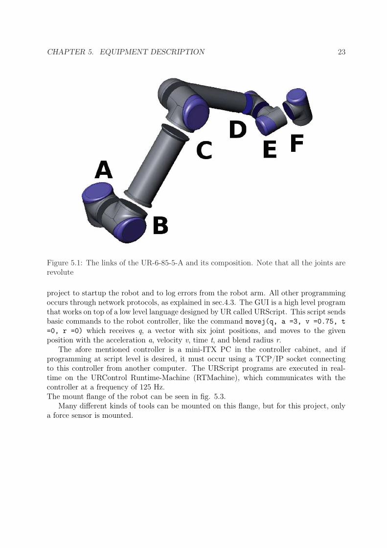
5.2 The UR-6-85-5-A robotThe Automation and Control group at DTU has received a 6-joint robot arm, from Uni-versal Robots, in Odense, which has been made available for students to make experimentsand do project work. The model of the robot is UR-6-85-5-A and is a light robot arm,weighing only 18 kg and capable of lifting up to 5 kg payloads. Details about the robotcan be found in the User Manual [Roba] and on the webpage www.universal-robots.com.Only a quick introduction will be given here. Fig. 5.1 shows the different parts of the URrobot:
• A: the base of the robot, where the robot is mounted
• B: the shoulder of the robot
• C: the elbow of the robot
• D,E,F: wrists 1,2, and 3 of the robot, where a tool is attached to the robot
By coordinating movement, the robot can move freely in 6 DOF with the constraintsshown in fig. 5.2, which shows that there is a cylindrical workspace along the robots baseZi axis, where the tool point cannot work. Also, the figure shows that the robots workingarea is a sphere of diameter 175 cm around the base.
The robot comes with a GUI called PolyScope which is easily programmable and allowspoint to point movement through the definition of wavepoints. This GUI is only used in this
3See chapter 3.2.1 in [OI09]
CHAPTER 5. EQUIPMENT DESCRIPTION 23
Figure 5.1: The links of the UR-6-85-5-A and its composition. Note that all the joints arerevolute
project to startup the robot and to log errors from the robot arm. All other programmingoccurs through network protocols, as explained in sec.4.3. The GUI is a high level programthat works on top of a low level language designed by UR called URScript. This script sendsbasic commands to the robot controller, like the command movej(q, a =3, v =0.75, t=0, r =0) which receives q, a vector with six joint positions, and moves to the givenposition with the acceleration a, velocity v, time t, and blend radius r.
The afore mentioned controller is a mini-ITX PC in the controller cabinet, and ifprogramming at script level is desired, it must occur using a TCP/IP socket connectingto this controller from another computer. The URScript programs are executed in real-time on the URControl Runtime-Machine (RTMachine), which communicates with thecontroller at a frequency of 125 Hz.The mount flange of the robot can be seen in fig. 5.3.
Many different kinds of tools can be mounted on this flange, but for this project, onlya force sensor is mounted.

CHAPTER 5. EQUIPMENT DESCRIPTION 24
Figure 5.2: The workarea of UR-6-85-5-A
Figure 5.3: The mounting flange of UR-6-85-5-A
Chapter 6
Implementation
6.1 Analysis of SolutionsThere are two different ways to approach the problem of converting the UR robot arm intoa deburring tool:
• To place a grinding machine on the end effector. This would allow the robot arm todeburr big objects which fit into the arms working area.
• To place a gripper tool, like a suction cup, on the end effector, and pass the desiredobject through deburring tools. This solution is focused on smaller objects, since thearm can only lift up to 5 kg with precision.
A comparison of the two methods for a solution has been made in table 6.1Each of these solutions has strengths and weaknesses, but the most important aspect
aimed at in this project is precision. If a grinding mill was to be used, the force sensor wouldnot be able to feel a steady push from the tool tip, since the mill would be shaving off piecesof the object to deburr. This would mean that the amount shaved off the object to deburrdepends on the precision of movement of the robot arm and the time of displacement ofthe tooltip. Since neither can be assumed to be reliable, the second method is concludedto be the best solution, see figure 6.1. In short, the solution consists of a controlled-pathrobot behaviour, combining joint and linear interpolation along with the force feedbackapproach.
6.2 Method ImplementationSince this project is only a testbench, the “suction cup method” is tested, without an activesuction cup, i.e. a victim element is placed on the end effector, simulating an element whichis attached to the end effector through a suction cup, see fig. 6.2. Furthermore, the element
1In tbl. 6.1 on the following page it is assumed that the density of steel is 7.8 g/cm3 [HDY04] and thus,the arm is capable of lifting a square plate with a thickness of 5 mm and sides of 35 cm.
25

CHAPTER 6. IMPLEMENTATION 26
Table 6.1: Method comparisonsTool mounted on Workpiece mountedend of robot on end of robot
Weight of object N/A 5 Kgto deburr
Reach of robot arm Radius of arm Depends on the weightand size of theobject to deburr
Size of object Must be inside the reach Depends on the weightto deburr of the robot arm of the object1
Precision of Depends on the odometry Depends on the forcedeburr process of the robot arm, since sensorand software code.
force sensor does not work The forcesensor permitseffectively with a adaptability,therefore,grinding mill.Therefore, high precisionis assumedlow precision is assumed.
Strength of Not necessarily soft All kind of materialsmaterial metals like aluminium as long as a gripper
can be designed
Speed Highest Higher than most machineor hand deburring processes
holders will not be built, but it is assummed that all elements are picked up at the exactlysame position with the same rotation.
For the proof of concept, it is assumed that the robot is standing in a production linewhere it has to deburr metal plates with the dimensions 10 cm × 15 cm Figure 6.3 showsa flowchart of how the robot deburrs all four sides of the elements. An element has beenmounted on the existing tool of the robot from the project [OI09]. The idea behind thissetup is to simulate a deburring process of four sides of this element in a model of a setuparound the robot. For this setup a model has been drawn for a deburring platform, seeappendix E on page 62. With help from the AUT department, this model was made inwood and mounted within the workspace of the robot. The model was mounted on a smalltable next to the robot in the lab, with clamps to prevent it from moving when the robotpushes the victim element against it. The robot was programmed to simulate the process ofpicking up the element, deburring its four sides, and then delivering the element for furtherwork elsewhere. The programming for this task will be discussed in chapter 7 on page 32.The tool chosen to be simulated is like the one in figure 4.1(b). The size of the tool isdetermined depending on the size of the element, which in this case is 10 cm × 15 cm, butthe size of the tool can easily be changed if the size of the workpiece should be changed. It

CHAPTER 6. IMPLEMENTATION 27
Figure 6.1: A simplified model of the theoretical setup of the deburring process
Figure 6.2: Test bench setup with an element attached to the robot tooltip
Figure 6.3: A flow chart of the deburring process
CHAPTER 6. IMPLEMENTATION 28
should be kept in mind that the size and speed of the cylinder doing the deburring dependson which material it should work on, how much material it should remove and how finethe result should be.
Appendix D on page 60 also shows a sketch of the victim element mounted on therobot. The mounting between the element, sensor and the robot is not included, sinceit was already made before this project started. The element ends up being mountedapproximately 10 cm from the center of the tool tip2 of the robot.
6.2.1 Deburr Process
The movements, before and after the element is near the deburring machine, are easy toprogram as point to point movements. This also includes the rotation of the victim elementto change side for deburring, and the position before the deburr process is started. Whilethe robot is to collect or deliver an element, the force sensor is used to make sure thatthe robot is pushed against the element or the element underneath before a vacuum isactivated or deactivated if a suction cup was implemented.
The elements ready to be picked up by the robot are to be placed in a holder where theelements are fixed in a precise position. In this way, the robot always picks up an elementin almost the same position. Due to programming, a small deviation of ±1 mm in thisposition is allowed. The position of the holder for unloading the plates does not have to bein a fixed position either. The holder is allowed to deviate in both rotation and positionby ± 1 mm.
In the position for deburring, no matter which side of the element is chosen for debur-ring, force measurements must be used for impact control and regulation. First, impactcontrol must be used to make the element move all the way to touch the deburring toolin two directions. The robot is programmed to move towards the deburring tool in onedirection, the Zs-direction of the force sensor, see fig. 6.4. This corresponds to a continousmovement along the Xr-axis and −Zr-axis of the robot, until the force sensor measures agiven reference value.
To complete the positioning of the element before the actual deburring is done, contacthas to be made with the rest of the sled of the deburring setup. This is completed bymoving the plate a 5 mm away from the machine and approaching the sled in the forcesensor’s −Xs-direction, which correspond to the −Xr-direction and −Zr-direction of therobot, until a force reference value is reached once more. Then the approach in the forcesensor’s Zs-direction is called once more to make the plate reach the sled as close as possible.
Fixed in the sled, the element is ready to be run by the deburring mill, which means theelement is moved along the robots Yr-axis, while it is pushed against the tool sled in theforce sensor’s Zs- and Xs-direction. The movement is controlled by a PI-regulator tryingto maintain a constant force in the Zs-direction. Position regulation along the Xr and Zr
axes is desired, and two PI-regulators maintain the wanted position along these two axes.When one side has been deburred, the robot deburrs three more sides before it is done
2TCP, Tool Center Point, named by UR

CHAPTER 6. IMPLEMENTATION 29
Figure 6.4: Model of approach to deburr tool. The Yr and Ys axis are chosen according tothe right hand rule. A spindle is
and ready to drop off the victim element again. In a production line, the element wouldbe turned upside down at the drop off point and put trough the process once more todeburr all eight edges, but this is outside of both our time line and main problem, and willtherefore be saved for future work.
6.2.2 Linear control design and kinematic values
The regulation used for the project was based on the hybrid-control used in [OI09]. Fig.6.5 shows a general block diagram of how the desired regulation is achieved. The idealsolution for the deburring process would have force regulation between the victim elementand the deburr platform on the robot’s Xr and Zr axes, see fig6.4.
The resulting system to be regulated would be of the multiple-input/multiple-output(MIMO) kind. This fact, paired up with torques and forces generated on the force sensordue to torsion when the victim element is not exactly aligned with the deburring sledge,results in the need of complicated regulation. The needed regulation is taught at DTU aspart of a masters course, and due to limitations on time, a simpler solution is chosen. Theregulation solution will have the following properties:
• Force feedback and regulation in the robot’s x- and z-axis
• Position feedback and regulation in the robot’s y- and z-axis
• A hybrid force/position regulation scheme
• A slightly underdamped system, which gives a better result

CHAPTER 6. IMPLEMENTATION 30
Figure 6.5: Block model of a hybrid force/position control scheme from [OI09]. Note thatthe forward kinematics are used to transform the joint positions θi to Cartesian coordinates,which are used as feedback for the position controller.
This regulation was achieved in the draw function of the python code, see chapter 7on page 32 for more information. The tuning of the values Kp and Ki was made by hand,trying different values, although the initial values were found using the Ziegler-Nicholscriteria, as described in [OI09].
The values for the Denavit-Hartenberg notation used are shown in table 6.2 The valuesare then inserted into the homogenous transform as stated in chapter 4.2 on page 15, andusing eq. (4.4) the homegenous transform 0T 6, which will be used in the programming formovement and location of the robot.

CHAPTER 6. IMPLEMENTATION 31
Table 6.2: Denavit-Hartenberg values used for the robot. They are obtained throughmeasurements made on the robot arm
i(frame) αi − 1 [◦] ai − 1 [m] di [m] θi
1 0 0 0.0892 θ1
2 90 0 0.1357 θ2
3 0 -0.42500 -0.1357 θ3
4 0 -0.39243 0.1090 θ4
5 90 0 0.0930 θ5
6 -90 0 0.0820 θ6

Chapter 7
Programming the robot
7.1 Functions and their usesThe code for this project builds upon the program from an earlier project, [OI09]. After ananalysis of this code, functions which were needed to complete the task had to be writtenor modified. Afterwards, all the functions which were no longer in use had to be erased.The purpose of the new functions are described on the flowchart in figure 6.3 on page 27.
These functions created with Python work as a high level programming language work-ing on top the URScript. There are two classes which were made:
• The force class, containing functions designed to retrieve information and removebias from the force sensor F.0.3
• The connection class, containing functions designed to speak with the robot, andthus send all movement scripts to the robot F.0.2
These two classes each have their own file, and a third file, called maindeburr.py F.0.1,serves as a primitive GUI. These three files can be seen in Appendix F, and can be analyzedif a detailed understanding of the different classes and functions is desired.
Mainly five kinds of tasks need to be scripted in order to do the deburring work:
Large movements in workspace These movements are made by establishing waypointswhere the robot arm has to stop. These points are called through the movej com-mand1
Approach with sensor feedback These functions were made by having loops movingthe tooltip in a desired direction, with the speedl script, while comparing the dataof the force sensor to a given reference value. In most cases this reference value was4 N. This kind of function is also used to simulate the pickup and delivering of theelements to be deburred
1For specific details on the working of these commands, refer to URscript Manual [Robb]
32

CHAPTER 7. PROGRAMMING THE ROBOT 33
Decoupling movements These movements are made with the speedl script, moving onlyshort distances away from the deburr setup. The original script was made by Ingólf-sson and Gudlaugsson, but this function is now divided into two different scripts,decoupling on different axes
Rotation of the tool point This is achieved by logging the current position of the jointsand then using the movej script to rotate wrist 3 of the robot. The rotation is madewith a slight bias due to the general position of the robot arm relative to the setup
Translation of the tool point with force regulation activated This is the most im-portant movement of the project, since it is the one that defines the precission of thedeburr work. This movement was achieved by creating a path, as described in chapter4.2.2, and continously sending the information from the force sensor and the posi-tion feedback through the PI-regulators. This was done in the draw function of theconnection class. The position feedback uses the forward kinematics in order to findthe Cartesian coordinates from the data received by the robot.
Since the victim element at the tool point creates a force bias due to gravity, the forcesensors bias needs to be removed after most of the movements are completed. This functionis defined in the force class.
Some of the used functions were already written by Ingolfsson and Gudlaugsson. Butmany of them are partially or completely rewritten in order to fit into this project, e.g. theoriginal approach function only moved in the Zs direction, parallel to the Xr-axis, whilethe rewritten one moves in a combination of Xr and Zr axes. The source code has beencommented in order to make clear which functions are based on Ingólfsson et. al. originalfunctions.
Two python-modules are loaded into the program: numpy and socket. Numpy, ornumerical python, is in charge of the mathematics and creating different matrices. Socketis in charge of TCP communication with the robot controller, and adding this module allowsto functions like socket.rcv and socket.send to be called. It is mainly due to the capabilitiesof this module that python was chosen as the programming language by Ingolfsson andGudlaugsson.
7.2 User manual for the programTo start up the program, it should first by assured that the robot, user-pc and sensor-pcare connected and are on the same network.
The IP-settings for the robot should be: IP:192.38.66.237 Subnet: 255.255.255.0, theIP-settings for the user-pc should be: IP:192.38.66.x2 Subnet: 255.255.255.0, and the IP-settings for the sensor-pc should be: IP:192.38.66.252 Subnet: 255.255.255.0. Control theconnection between the sensor and the sensor pc is plugged in correctly.
2x should be a number between 1-255, except 252 and 237

CHAPTER 7. PROGRAMMING THE ROBOT 34
Then the Visual Basic 6 script written for [OI09] on the sensor PC should be started,press the following buttons: Listen, Initialize sensor, Remove bias, and Fetch data. Thelast one is to check that everything is working, and if the data is not close to zero it mightsuggest an error.
Turn on the robot, follow the text on the screen to initialize it. Remove anythingwithing 20 cm of the robot arm before turning the power on and be careful not to hitanything while moving the arm, during this stage.
When the robot is initialized, choose “Program Robot” on the main screen and go tothe Log tab. This will help understanding any problem, if one should occur. Make surethe Ethernet controller does not have packet loss at this stage, otherwise restart the robotright away. Now it is possible to start the user interface at the user-pc. Make sure thatthe user-pc has Python version 2.5 and the source code from this project. Start the filecalled maindeburr.py from Appendix F.0.1, on Microsoft Windows 2000 or newer. Thiscan be done by a double click on the file or by running the file in a command window. InUnix/Linux systems it can be run in a terminal window.
The program will start moving the robot to the first position and when it is done, themain screen will show, see figure 7.1. The following choices are possible:deburr Choosing this will make it possible for the user to choose how many elements to
deburr and then start the process. The maximum number of elements is 10 pieces.
debug Choosing this will make it possible for an advanced user to access the temporarymenu, used to do the programming. This menu is partly a copy of the one use by[OI09] with a few extra options
exit Choosing this will shut down the program, after closing any open files or sockets
Figure 7.1: Mainscreen for the user interface at the user pc connected to the robot controllerand sensor pc
Before any use of the robot always read the safety instruction in the user manual for therobot [Roba].
Chapter 8
Calibration and Test
This chapter shows how the solution for the given problem was tested and how the instru-ments were calibrated in order to get precise and accurate measurements. Further, thecollected graphs and data, are discussed and compared.
8.1 Test of communication speedIngólfsson and Gudlaugsson observed that communication over Ethernet between the con-trol PC, sensor PC and the robot not always worked as described in the data sheet of therobot. The sensor PC did not show problems of communication, due to the fact that itdoes not communicate with the robot, but only with the sensor and the control PC. Amodel of the network can be seen in figure 8.1.
In the script manual [Robb] of the robot it is stated that the robots real time Run-timeMachine1 can handle communication at a speed of 125 Hz. This frequency has provento be difficult to mantain while running communication over Ethernet. The robot crashedwith the error “No Controller”2 and stopped if calls were sent at this rate. By restrictingthe send rate to 41 Hz, the crash error was prevented from occurring everytime. This crasherror still appears sporadically, without any clear reason.
To test the controller crash problem, a small piece of code was designed to call one ofthe UR Script commands at a determined rate. This also gave an opportunity to learnmove about the UR Script. The random() command was chosen, because the robot doesnot have to move for this command to work and thereby does not have to ensure that italways stays inside its own workspace. This command is also supposed to return a valueto the control PC, like most of all other commands that move the robot.
This small program consist of a “while” loop, where the speed of the loop can becontrolled to determine the frequency of the call of the socket.send() command. The ideawas then to run the loop at different frequencies and see how long it would run without
1See chapter 5.2 on page 222In the log: PolyScope disconnected from Controller
35

CHAPTER 8. CALIBRATION AND TEST 36
Figure 8.1: A model of the network around the robot
getting the error on the touchscreen of the robot. To determine if this command actuallyreached the robot and the robot answered, a program was included in the loop, which wrotethe answer from the robot with a time stamp to a file. This file did work, but the answerfrom the robot was not as expected, since it consisted of the position of the robot and not arandom number from 0-1 as the UR Script manual stated. Also, the time stamp to controlthe frequency in the text file was not working as planed and needed reprogramming to besure it was accurate.
Due to the failure of completion of this test, the project was continued with restrictionson the communication speed. This means that when a movement is done which dependson a read-out from the force sensor, the frequency for every socket.send() command call tothe robot is locked to 41 Hz, as in [OI09].
The only function not having the same frequency restriction is the approach_z_x, whichhas even more strict limitations on the speed of the socket.send() calls.
8.2 Force feedback during deburrThe read-out of the force sensor was logged for analysis purposes and can be seen in fig.8.2.
From this graph, it is clear that regulation toward a force reference of 4 N is achieved.The graph shows the force feedback each time a side of an element is passed throughthe deburr setup. It is also quite clear here, that the force regulation is very sensitive

CHAPTER 8. CALIBRATION AND TEST 37
0 10 20 30 40 50 60−2
0
2
4
6
8
10
12
14
16
Time
Z [N
]
Actual ForceReference Force
Figure 8.2: Force feedback during the deburring of the four sides of an element. The first,third and fourth deburr maintain a stable pressure agains the deburr sledge
to the start position of the robot, and whether the victim element is completely alignedwith the debur sledge or not. The first, third and fourth runs maintain an even forceregulation, while the second loses its grip against the deburr sledge. This happens becausethe alignment angle between the sledge and element is too big when the element is rotatedinto the second position for deburring. This could be solved by having a tool tip which isable to bend and adapt a few degrees, so the plate ends up being completely flat againstthe deburr sledge.
8.3 Noise on the force sensorThe force sensor used in this project has been described in chapter 5.1 on page 21 andit has been noted that it had an unpredictable error, which showed as a a peak read-outof a force larger than what the sensor should be able to measure. In the Appendix A onpage 46 sets of data are listed, containing information read out from the force sensor innine different positions in the workspace of the robot:
• Random position
• Deburr positions 1− 4, just before the robot starts moving towards the deburr setup
• Initialize position
• Stretched out horizontal, with the tool at maximum reach, downward, and upward

CHAPTER 8. CALIBRATION AND TEST 38
In each data set there are values which are out of the measuring range of the forcesensor. It should be noted that the sensor cannot measure more than ±40 N of force inthe x-axis and y-axis, and ±120 N of force in the z-axis, see table 5.1 on page 22. Thedata received reaches numbers up to ±255 N or even ±256 · 108 N, and this error is notconnected to only one axis.
These peak errors have to be removed from the data sent to the system, otherwise thecorrections for the robots movements can be fatal for the equipment and setup. Still, thesetup has completed the deburr process of 10 elements in a row without crashing or havingserious errors.
−0.2
0
0.2
0.4
0.6First deburr position
For
ce o
n th
e X
−ax
is [N
]
Actual F.Reference F.Maximum & Minimum
−4
−2
0
2
For
ce o
n th
e Y
−ax
is [N
]
Actual F.Reference F.Maximum & Minimum
0 500 1000 1500−0.1
0
0.1
0.2
0.3
Sample point
For
ce o
n th
e Z
−ax
is [N
]
Actual F.Reference F.Maximum & Minimum
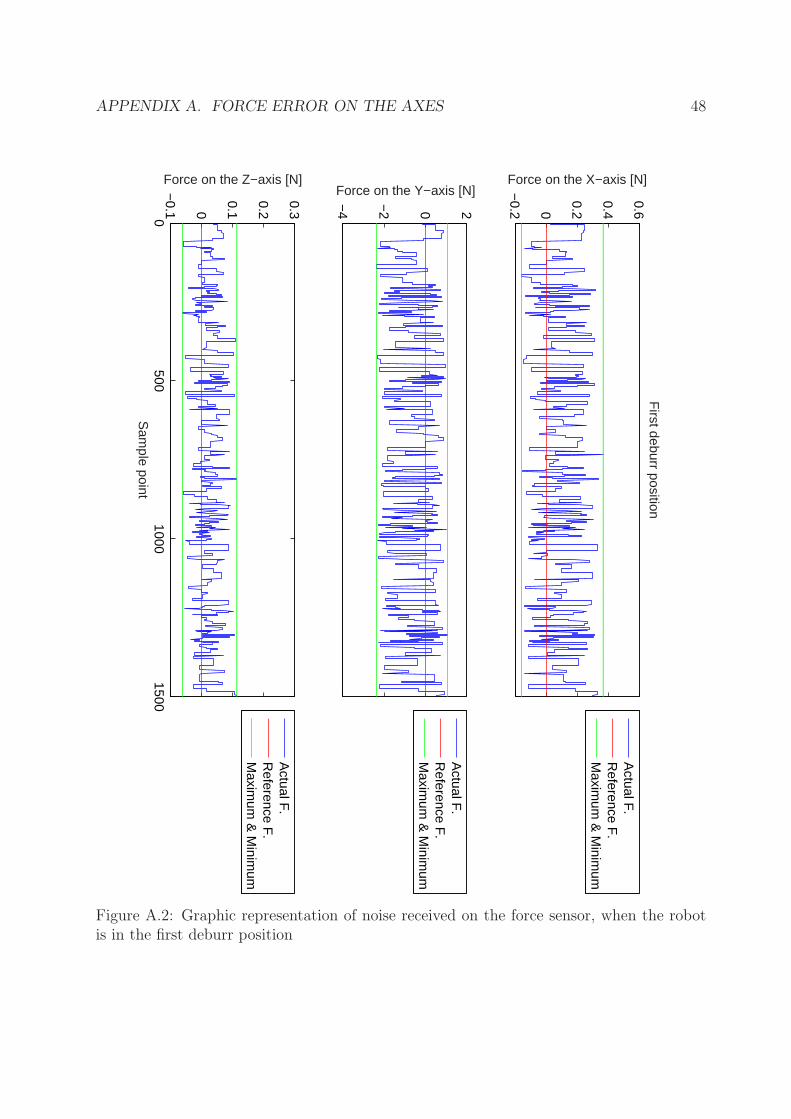
Figure 8.3: Graphic representation of noise recieved on the force sensor, when the robot isin the first deburr position, see also Appendix A
With the high peak errors removed from the data sets, the force sensor still experienceserrors, but smaller than ±2 N. This can be seen in figure 8.3. The figure show forcemeasurements from all three axis at the moment where the robot is at a waypoint, justbefore it starts deburring the first edge of an elelement.
If these numbers are compared to the rest of the measurements in the Appendix Ait is apparent that the force sensing depends on when exactly the force bias is removedfrom all three axis. It is concluded that the measured noise comes from the robot. Whilestanding still in a position in space and turned on, the robot will always vibrate a littleand this movement is measured by the force sensor. The vibrations come from the motorsin the robot, which are trying to hold the robot still in the preprogrammed position whileworking against gravity. The hight vibration measurements are due to the weight of theelement at the tool tip, which amplifies the error readings at the sensor.

CHAPTER 8. CALIBRATION AND TEST 39
When the robot moves there is also noise on the sensor, but this phenomenon has notbeen analyzed in this project. When the force sensor is used throughout this project, thenoise coming from the vibrations of the robot has been discarded as always being within amargin of ±4N during a move through the deburr tool. This can be seen in section 8.2 onpage 36. During the project, this noise has been taken into account regarding the linearcontrol, which led to the use of a PI-regulator instead of a PID-regulator3.
In [OI09] noise problems were minimal due to the small weight of the tool on the tip ofthe sensor. This noise was not taken into account since most of the noise came from thecontact point between the chalk and the surface of the chalkboard or between the peg andthe block of tree with a hole.
3See chapter 4.4 on page 19

Chapter 9
Errors in the robot
The robot used in this project is a prototype model used for tests inside UR. This means,it was built as one of the first of its type and some parts of the robot and its controls mayhave changed in newer version. This section will explain some of the problems which wereencountered throughout this project.
When the robot is being turned on for the first time after long period of inactivity, itdoes not always work and needs to be restarted. The error consists in some kind of failurein the Ethernet card or driver, which does not start up the Ethernet properly. The logstates “Ethernet 001 Packets loss”, which does not explain much, but implies that the errorlies in the network communication drivers of the robot.
Another error comes after the control box for the robot has been moved. The wires forthe touchscreen might be moved as well and an error occurs with the touchscreen, makingit impossible to control the robot without an external mouse or keyboard. This error hasnot been present all the time, but appears due to wear and tear on the wires which go intothe control box. When these wires were installed at UR, nothing was used to prevent thesharp edges of the control box to cut into the wires, and if a closer look is taken, it is nowpossible to see through most of the isolation cap and into the cores or shields of almost allthe wires.
This model was not meant to be transported, moved or placed in an environment whichvibrates in any way. This limitation has not been commented to the AUT group, or anystudent working with the robot. The limitation became apparent when the log suddenlyone morning simply stated “48 V Internal power supply is at 0V” at start up. The robothad the day before shown no problems when turned off. Universal Robots was contactedand the problem was explained. The solution was that the control box should be takenapart an examined at DTU, rather than sending it to Odense and back, which could havetaken weeks off the projects time schedule.
When taken apart, it was clear what was wrong: one wire from the 48 V Internal powersupply had been torn out from its socket on the main controller board. This apparentlyhappened due to the length of the wire and vibrations between the power supply and themain controller board. While the controller was taken apart it was also noted that twoout of three ceramic resistors had almost broken completely off. This also occurred due to
40

CHAPTER 9. ERRORS IN THE ROBOT 41
vibrations, and because the resistors had not been mounted correctly, but had only beeninstalled in a socket in one end. The weight of each resistor had then been enough to moveit around every time the controller box was shaken or moved due to gravity. After sometime, the wires connecting the resistances must have become weak and broken off.
Representative of UR stated that the resistors are used to burn off energy when therobot is deaccelerating and no damage should have been done as long as the robot had notbeen used intensively over a long period. Two new resistors were sent from Odense andinstalled upon arrival, this time secured by strips to avoid the same error again later on.UR claims that this construction error has now been corrected.
In section 8.1 on page 35 an error concerning the controller crashing has been explained.During the project, this error has appeared on different occasions, and was mentioned toUR. It was discussed if the heat that building up inside the controller box could affect thecontrollor. UR insisted that is was not the case, because the temperature should not riseabove the maximum working temperature for all the components inside the controller box.

Chapter 10
Conclusion
Throughout the realization of this project, several branches of engineering and tools havebeen used. Programming, linear control, physics and mathematics are among the mostprominent, and they were all used together to achieve a result. This result is the creationof a test bench which proves that a robot arm UR-6-85-5-A is able to deburr four sides ofa metal plate (victim element) using a force sensor installed on its tool tip. A setup wascreated to simulate the deburring process, which is divided into the following steps:
1. The user chooses how many elements are to be deburred
2. The robot arm simulates picking up an element with a suction cup
3. Using force regulation in order to follow a surface, the robot passes the victim ele-ments four sides by a mock-up of a deburring machine
4. The robot arm simulates delivering the deburred plate at a given position
5. The robot repeats the procedure if necessary
Programming was made with the Python language, and proved to be very effective to thetask. It eased the use of the URScript language and communication with the robot arm.Force regulaton was achieved through the use of a PI-regulator acting in the software. Itregulated along the Z-axis of the sensor, and proved to be moderately adequate for thetask. Other control techniques might have been better for force regulation in two axes, butknowledge of those techniques was outside the scope of this project.The solution is not as precise as it was hoped it could be. This stems from the fact thatonly force regulation in one axis was achieved. At the same time, a solution was expectedto be found for removing/dampening the vibrations generated by the robot, but they onlybecame worse due to the heavy weight on the tool tip.The team is satisfied with the knowledge acquired during this project, and with the resultsachieved.
42

Chapter 11
Future Work
Throughout this project, more problems have been revealed during the search for solutionsto the stated questions in the problem statement. Some of these have been outside theframe of this project, others were too time consuming, and some have had to be discardeddue to the lack of the knowledge needed to solve the problem.
The following points are tasks or problems which could be solved in the future as aspecial course, or simply for the challenge:
Change in size of the elements to be deburred The product of this project can bemade to take an input of the dimensions of the victim elements and thereby adjustall the waypoints in the procedure to take the dimensions into account before movingfrom waypoint to waypoint
Improving the use of the deburr tools As described in 4.1 on page 9 the wear andtear on the deburr tool will make the deburring less precise for every run, and atsome point the tool needs to be sharpened or replaced. When a tool has been chosen,the amount runs before the tool needs to be changed has to be determined, if the toolmanufacturer has not stated this already. A solution to extend the life of a tool canbe to made through a mechanism that moves the angle of attack on the tool betweenor during each run
Deburring all eight sides of an element Another future feature can be to design aregrip fixture for the setup inorder to make the robot capable of deburring all eightedges of a victim element
Expansion of the control to force feedback in several axes The SISO system de-veloped in this project can be optimized into a multiple input/multiple out (MIMO)system that is able to use force feedback from all axes of the sensor or even the torqueoutputs. This would make the victim elements follow all the sides of the modelleddeburr tool even smoother
Noise reduction A filtering system can be built inorder to remove even more noise fromthe force sensor at the TCP of the robot. This would make the controlled movements
43

CHAPTER 11. FUTURE WORK 44
even smoother
Completion of test setup The setup can be completed adding a suction cup at the tooltip and a vacuum system mounted near the robot. Also the holders beside the robotfor the arriving and leaving victim elements can be designed and put into the setup.A real grinding mill could be installed too, although some security measure shouldbe established

Bibliography
[A.] ATI I. A. Mini40-r. On-line, http://www.ati-ia.com/products/ft/ft_models.aspx?id=Mini40.
[Cra04] John J. Craig. Introduction to Robotics - Mechanics and Control. Prentice Hall,3rd edition, 2004.
[CW76] Raymond F. Veilleux Charles Wick. Tool and Manufacturing Engineers Hand-book: Materials, Finishing, and Coating, volume III, chapter 16. McGraw-HillBook Co., 1976.
[Eis99] Jens Eising. Lineaer Algebra. Institut for Matematik, DTU, 1999.
[Gil99] LaRoux K. Gillespie. Deburring and edge finishing handbook. Asme Books, 1999.
[Har] Tom Harris. How robots work. How Stuff Works. On-line,http://science.howstuffworks.com/robot2.htm.
[HDY04] Roger A. Freedman Hugh D. Young. University Physics with Modern Physics,chapter 14, page 516. Pearson Addison Wesley, 11 edition, 2004.
[Iso05] James Isom. A brieg history of robotics. On-line,http://robotics.megagiant.com/history.html, 2002-2005.
[MWS05] Mathukumalli Vidyasagar Mark W. Spong, Seth Hutchinson. Robot Modelingand Control, chapter 3, page 496. Wiley, 2005.
[OI09] Einir Gudlaugsson Örn Ingólfsson. Flexible control of a robot arm using sensorfeedback. Master’s thesis, DTU Electrical Engineering, July 2009.
[OJ06] Paul Haase Soerensen Ole Jannerup. Reguleringsteknik. Polyteknisk Forlag, 4thedition, 2006.
[Roba] Universal Robots. UR-6-85-5-A Users Manual. Universal Robots, On-line(PDF), http://www.universal-robots.com/, 1.1 edition.
[Robb] Universal Robots. The URScript Programming Language. Universal Robots,On-line (PDF),www.universal-robots.com.
45

Appendix A
Force error on the axes
46

APPENDIX A. FORCE ERROR ON THE AXES 47
−4
−2 0 2
Random
position of the robot
Force on the X−axis [N]
A
ctual F.
Reference F
.M
aximum
& M
inimum
−2
−1 0 1 2
Force on the Y−axis [N]
A
ctual F.
Reference F
.M
aximum
& M
inimum
0500
10001500
−0.5 0
0.5 1
Sam
ple point
Force on the Z−axis [N]
A
ctual F.
Reference F
.M
aximum
& M
inimum
Figure A.1: Graphic representation of noise received on the force sensor, when the robotis in a random position
APPENDIX A. FORCE ERROR ON THE AXES 48
−0.2 0
0.2
0.4
0.6F
irst deburr position
Force on the X−axis [N]
A
ctual F.
Reference F
.M
aximum
& M
inimum
−4
−2 0 2
Force on the Y−axis [N]
A
ctual F.
Reference F
.M
aximum
& M
inimum
0500
10001500
−0.1 0
0.1
0.2
0.3
Sam
ple point
Force on the Z−axis [N]
A
ctual F.
Reference F
.M
aximum
& M
inimum
Figure A.2: Graphic representation of noise received on the force sensor, when the robotis in the first deburr position

APPENDIX A. FORCE ERROR ON THE AXES 49
−3
−2
−1 0 1
Second deburr position
Force on the X−axis [N]
A
ctual F.
Reference F
.M
aximum
& M
inimum
−0.4
−0.2 0
0.2
0.4
Force on the Y−axis [N]
A
ctual F.
Reference F
.M
aximum
& M
inimum
0500
10001500
−0.1
−0.05 0
0.05
0.1
Sam
ple point
Force on the Z−axis [N]
A
ctual F.
Reference F
.M
aximum
& M
inimum
Figure A.3: Graphic representation of noise received on the force sensor, when the robotis the second deburr position

APPENDIX A. FORCE ERROR ON THE AXES 50
−0.6
−0.4
−0.2 0
0.2T
hird deburr position
Force on the X−axis [N]
A
ctual F.
Reference F
.M
aximum
& M
inimum
−4
−2 0 2
Force on the Y−axis [N]
A
ctual F.
Reference F
.M
aximum
& M
inimum
0500
10001500
−0.2
−0.1 0
0.1
0.2
Sam
ple point
Force on the Z−axis [N]
A
ctual F.
Reference F
.M
aximum
& M
inimum
Figure A.4: Graphic representation of noise received on the force sensor, when the robotis in the third deburr position

APPENDIX A. FORCE ERROR ON THE AXES 51
−4
−2 0 2
Fourth deburr position
Force on the X−axis [N]
A
ctual F.
Reference F
.M
aximum
& M
inimum
−0.2 0
0.2
0.4
0.6
Force on the Y−axis [N]
A
ctual F.
Reference F
.M
aximum
& M
inimum
0500
10001500
−0.1
−0.05 0
0.05
0.1
Sam
ple point
Force on the Z−axis [N]
A
ctual F.
Reference F
.M
aximum
& M
inimum
Figure A.5: Graphic representation of noise received on the force sensor, when the robotis in the fourth deburr position

APPENDIX A. FORCE ERROR ON THE AXES 52
−0.6
−0.4
−0.2 0
0.2Init position
Force on the X−axis [N]
A
ctual F.
Reference F
.M
aximum
& M
inimum
−4
−2 0 2
Force on the Y−axis [N]
A
ctual F.
Reference F
.M
aximum
& M
inimum
0500
10001500
−0.2
−0.1 0
0.1
0.2
Sam
ple point
Force on the Z−axis [N]
A
ctual F.
Reference F
.M
aximum
& M
inimum
Figure A.6: Graphic representation of noise received on the force sensor, when the robotis in the initialize position

APPENDIX A. FORCE ERROR ON THE AXES 53
−2
−1 0 1
Horizontal stretch of the robot
Force on the X−axis [N]
A
ctual F.
Reference F
.M
aximum
& M
inimum
−4
−2 0 2
Force on the Y−axis [N]
A
ctual F.
Reference F
.M
aximum
& M
inimum
0500
10001500
−0.5 0
0.5
Sam
ple point
Force on the Z−axis [N]
A
ctual F.
Reference F
.M
aximum
& M
inimum
Figure A.7: Graphic representation of noise received on the force sensor, when the robotis in a horizontal stretched position with the tool pointing outward

APPENDIX A. FORCE ERROR ON THE AXES 54
−1 0 1 2 3
Horizontal stretch of the robot, the tool turned dow
nward
Force on the X−axis [N]
A
ctual F.
Reference F
.M
aximum
& M
inimum
−2
−1 0 1 2
Force on the Y−axis [N]
A
ctual F.
Reference F
.M
aximum
& M
inimum
0500
10001500
−0.2 0
0.2
0.4
0.6
Sam
ple point
Force on the Z−axis [N]
A
ctual F.
Reference F
.M
aximum
& M
inimum
Figure A.8: Graphic representation of noise received on the force sensor, when the robotis in a horizontal stretched position with the tool pointing downward

APPENDIX A. FORCE ERROR ON THE AXES 55
−1 0 1 2
Horizontal stretch of the robot, the tool turned upw
ard
Force on the X−axis [N]
A
ctual F.
Reference F
.M
aximum
& M
inimum
−2
−1 0 1 2
Force on the Y−axis [N]
A
ctual F.
Reference F
.M
aximum
& M
inimum
0500
10001500
−0.5 0
0.5
Sam
ple point
Force on the Z−axis [N]
A
ctual F.
Reference F
.M
aximum
& M
inimum
Figure A.9: Graphic representation of noise received on the force sensor, when the robotis in a horizontal stretched position with the tool pointing upward

Appendix B
CD List of Contents
9230-05-1278.pdf Drawning of the Mini40-R force sensor
BondyS051976-WahlgreenS042157.pdf Copy of the report with signatures
connectionregulatortest.py Program for all communication between the user-pc andthe robot controller
Drawing - deburr.igr Drawing of the model of the deburr tool, opens in SmartSketch
Drawing - deburr.pdf Drawing of the model of the deburr tool
Drawing - tool.igr Drawing of the victim element, opens in SmartSketch
Drawing - tool.pdf Drawing of the victim element, opens in SmartSketch
force.py Program for all communication between the user-pc and the sensor-pc
force_test.py Test program, which reads out data from the sensor for analyze
force_test.txt Test data from force sensor, random position
force_test_deburr1.txt Test data from force sensor, 1(st) side position
force_test_deburr2.txt Test data from force sensor, 2(nd) side position
force_test_deburr3.txt Test data from force sensor, 3(rd) side position
force_test_deburr4.txt Test data from force sensor, 4(th) side position
force_test_init.txt Test data from force sensor, init position
force_test_stretch.txt Test data from force sensor, horizontal stretch of robot withtool at maximum range
force_test_stretch_down.txt Test data from force sensor, horizontal stretch of robotwith tool downward
56

APPENDIX B. CD LIST OF CONTENTS 57
force_test_stretch_up.txt Test data from force sensor, horizontal stretch of robotwith tool upward
maindeburr.py Main program file
scriptmanual_en.pdf URScript Manual from UR
testit_fourthrun.txt Test data from force sensor, while deburring one element
UR-6-85-5-A_Produktblad_web_UK.pdf Datasheet for the UR–6–85–5–A

Appendix C
Drawing of force sensor
58

APPENDIX C. DRAWING OF FORCE SENSOR 59
Figure C.1: Technical drawing of the force sensor [A.]

Appendix D
Drawing of the victim element
60

APPENDIX D. DRAWING OF THE VICTIM ELEMENT 61
Figure D.1: Technical drawing the victim element, Not in scale, see B

Appendix E
Drawing of the deburr tool model
62

APPENDIX E. DRAWING OF THE DEBURR TOOL MODEL 63
Figure E.1: Technical drawing no. 1 of the deburr tool model, Not in scale, see B

APPENDIX E. DRAWING OF THE DEBURR TOOL MODEL 64
Figure E.2: Technical drawing no. 2 of the deburr tool model, Not in scale, see B

Appendix F
Source code
F.0.1 maindeburr.py
# −∗− coding : cp1252 −∗−
de f sy s t emc l ea r ( ) : #This c l e a r s the s c r e en depending on the OS usedimport osi f os . name == "pos ix " :# Unix/Linux/MacOS/BSD/ etc
os . system ( ’ c l e a r ’ )e l i f os . name in (" nt " , "dos " , " ce " ) :# DOS/Windowsos . system ( ’CLS ’ )
import numpyfrom numpy import ∗import timeimport l o c a l el o c a l e . s e t l o c a l e ( l o c a l e .LC_NUMERIC, ’ ’ )from conn e c t i o n r e gu l a t o r t e s t import Connectionfrom f o r c e import Forcec = Connection ( ’ 1 9 2 . 3 8 . 6 6 . 2 3 7 ’ , 30003)t = 0whi l e ( t==0):
sy s t emc l ea r ( )p r i n t "Moving robot in to s t a r t po s i t i on , p l e a s e wait "c . i n i t i a l i z e ( )sy s t emc l ea r ( )f = Force ( ’ 1 9 2 . 3 8 . 6 6 . 2 5 2 ’ , 12345)f . b i a s ( )c . i n i t_va r i a b l e s ( 4 , 0 . 0 2 , 0 . 0 005 , 1 )
65

APPENDIX F. SOURCE CODE 66
p l a t e s = 1pr in t ""p r i n t "#################################"pr in t "### Welcome to ###"pr in t "### the deburr program ###"pr in t "#################################"pr in t ""p r i n t "The commands f o r t h i s program are : "p r i n t " deburr = Star t deburr ing "p r i n t " debug = Enter debug menu"pr in t " e x i t = Exit the program"pr in t ""p r i n t " I f no or a wrong input i s g iven "p r i n t "you w i l l r e turn to t h i s s c r e en "p r i n t ""cho i c e = raw_input ("Command: ")p r i n t ""
i f cho i c e == "deburr " :p l a t e s = raw_input ("How many p l a t e s should be deburred ? (MAX 10 ) : ")t ry :
p l a t e s = f l o a t ( p l a t e s )except Exception , e :
p r i n t "Error ! " , e , " Please make sure you put in a number between 1−10"e x i t ("\nTry s t a r t i n g the program again \n")
i f p l a t e s > 10 :p r i n t ""p r i n t "#################################"pr in t "### Deburring p l a t e s 10 ###"pr in t "#################################"pr in t ""p l a t e s = 10
e l i f p l a t e s <= 0 :p r i n t ""p r i n t "#################################"pr in t "### NOT Deburring any p l a t e s ###"pr in t "#################################"pr in t ""time . s l e e p (3 )
deburred_plates = 0sys t emc l ea r ( )whi l e deburred_plates < p l a t e s :
p r i n t ""

APPENDIX F. SOURCE CODE 67
p r i n t "#################################"pr in t "### Plate no %s i s running ###" % s t r ( deburred_plates+1)p r i n t "#################################"pr in t ""g l oba l turncounterturncounter = 0c . c o l l e c t ( turncounter )c . deburr ( turncounter )c . d e l i v e r ( )deburred_plates = deburred_plates + 1
c . i n i t i a l i z e ( )sy s t emc l ea r ( )p r i n t ""p r i n t "##################################"pr in t "### Fini shed deburr ing p l a t e s ###"pr in t "##################################"pr in t ""
i f cho i c e == "debug " :t = 1
i f cho i c e == " ex i t " :sy s t emc l ea r ( )t ry :
my f i l eexcept NameError :
my f i l e = None
try :myf i l e2
except NameError :myf i l e2 = None
try :myf i l e3
except NameError :myf i l e3 = None
i f my f i l e i s None :my f i l e = 1
e l s e :#pr in t "Test : %s " % myf i l e . c l o s ed

APPENDIX F. SOURCE CODE 68
myf i l e . c l o s e ( )#pr in t "Myf i l e i s c l o s ed "
i f myf i l e2 i s None :my f i l e = 1
e l s e :#pr in t "Test : %s " % myf i l e . c l o s edmyf i l e2 . c l o s e ( )#pr in t "Myf i l e2 i s c l o s ed "
i f myf i l e3 i s None :my f i l e = 1
e l s e :#pr in t "Test : %s " % myf i l e . c l o s edmyf i l e3 . c l o s e ( )#pr in t "Myf i l e3 i s c l o s ed "
c . connect ( )c . c l o s e ( )e x i t ("\nBuy\n")
cho i c e = ""
#Debugmode , the o ld i n t e r f a c e adopted pa r t l y from Orn & Ein i rwhi l e ( 1 ) :
p r i n t "pos − d i sp l ay cur r ent robot p o s i t i o n "p r i n t " i n i t − i n i t i a l i z e the robot "p r i n t " f o r c e − cur r ent f o r c e read ing "p r i n t " b i a s − remove f o r c e b i a s "p r i n t " goto − goto c a r t e s i a n po s i t i o n "p r i n t "move − t r a n s l a t e end e f f e c t o r "p r i n t " t e s t − Rotation t e s t movement from python"pr i n t "random − t e s t i n g o f c o n t r o l l e r speed , not working proper ly "p r i n t " e x i t − e x i t s program"pr in t "approachx− f o r t e s t i n g purpose only "p r i n t "approachy− f o r t e s t i n g purpose only "p r i n t " c o l − Co l l e c t p l a t e "p r i n t " de l − De l i v e r p l a t e "p r i n t "deburr − Deburr program"s e l e c t i o n = raw_input (" Enter your s e l e c t i o n : ")

APPENDIX F. SOURCE CODE 69
i f s e l e c t i o n == " i n i t " :sy s t emc l ea r ( )g l oba l co s tp r i n t ""p r i n t "#########"pr in t " i n i t i a l i z i n g robot "p r i n t "#########"pr in t ""import timec . i n i t i a l i z e ( )f = Force ( ’ 1 9 2 . 3 8 . 6 6 . 2 5 2 ’ , 12345)f . b i a s ( )c . i n i t_va r i a b l e s ( 2 , 0 . 0 3 , 0 . 0 015 , 1 )p r i n t " Please wait u n t i l the robot has stopped moving , be f o r e c a l l i n g a new command"pr in t ""
i f s e l e c t i o n == " b ia s " :sy s t emc l ea r ( )p r i n t ""p r i n t "#########"pr in t " i n i t i a l i z i n g Force Sensor "p r i n t "#########"pr in t ""f = Force ( ’ 1 9 2 . 3 8 . 6 6 . 2 5 2 ’ , 12345)f . b i a s ( )
i f s e l e c t i o n == "goto " :sy s t emc l ea r ( )c . e s tab l i sh_connec t i on ( )r e s u l t s = c . read_socket_stream ( )f = c . forward_kin ( r e s u l t s . va lue s [ 3 0 ] , r e s u l t s . va lue s [ 3 1 ] , r e s u l t s . va lue s [ 3 2 ] , r e s u l t s . va lue s [ 3 3 ] , r e s u l t s . va lue s [ 3 4 ] , r e s u l t s . va lue s [ 3 5 ] )p r i n t ""p r i n t "#########"pr in t "Current robot p o s i t i o n i s : [%.6 f ,%.6 f ,%.6 f ] " %( f [ 0 ] , f [ 1 ] , f [ 2 ] )p r i n t "#########"pr in t ""x = raw_input (" Enter X coord ina te [m] : ")y = raw_input (" Enter Y coord ina te [m] : ")z = raw_input (" Enter Z coord ina te [m] : ")c . send_cartes ian_to_socket ( f l o a t ( x ) , f l o a t ( y ) , f l o a t ( z ) )sy s t emc l ea r ( )

APPENDIX F. SOURCE CODE 70
i f s e l e c t i o n == "move " :sy s t emc l ea r ( )c . e s tab l i sh_connec t i on ( )r e s u l t s = c . read_socket_stream ( )f = c . forward_kin ( r e s u l t s . va lue s [ 3 0 ] , r e s u l t s . va lue s [ 3 1 ] , r e s u l t s . va lue s [ 3 2 ] , r e s u l t s . va lue s [ 3 3 ] , r e s u l t s . va lue s [ 3 4 ] , r e s u l t s . va lue s [ 3 5 ] )c . c l o s e ( )x = raw_input (" Enter X disp lacement [m] : ")y = raw_input (" Enter Y disp lacement [m] : ")z = raw_input (" Enter Z disp lacement [m] : ")c . i n i t_va r i a b l e s ( 2 , 0 . 0 3 , 0 . 0 015 , 1 )c . t r a n s l a t e ( f l o a t ( x ) , f l o a t ( y ) , f l o a t ( z ) , 0 , 0 , 0 )c . e s tab l i sh_connec t i on ( )r e s u l t s = c . read_socket_stream ( )f2 = c . forward_kin ( r e s u l t s . va lue s [ 3 0 ] , r e s u l t s . va lue s [ 3 1 ] , r e s u l t s . va lue s [ 3 2 ] , r e s u l t s . va lue s [ 3 3 ] , r e s u l t s . va lue s [ 3 4 ] , r e s u l t s . va lue s [ 3 5 ] )c . c l o s e ( )p r i n t "Total movement was : [%.4 f ,%.4 f ,%.4 f ] " %( f2 [0]− f [ 0 ] , f 2 [1]− f [ 1 ] , f 2 [2]− f [ 2 ] )
i f s e l e c t i o n == "pos " :sy s t emc l ea r ( )c . e s tab l i sh_connec t i on ( )r e s u l t s = c . read_socket_stream ( )f = c . forward_kin ( r e s u l t s . va lue s [ 3 0 ] , r e s u l t s . va lue s [ 3 1 ] , r e s u l t s . va lue s [ 3 2 ] , r e s u l t s . va lue s [ 3 3 ] , r e s u l t s . va lue s [ 3 4 ] , r e s u l t s . va lue s [ 3 5 ] )c . c l o s e ( )my f i l e = open (" data . txt " , "a ")my f i l e . wr i t e ("%.17 f ,%.17 f ,%.17 f ,%.17 f ,%.17 f ,%.17 f \n" %( r e s u l t s . va lue s [ 3 0 ] , r e s u l t s . va lue s [ 3 1 ] , r e s u l t s . va lue s [ 3 2 ] , r e s u l t s . va lue s [ 3 3 ] , r e s u l t s . va lue s [ 3 4 ] , r e s u l t s . va lue s [ 3 5 ] ) )my f i l e . c l o s e ( )p r i n t ""p r i n t "#########"pr in t "Current robot p o s i t i o n i s : [%.6 f ,%.6 f ,%.6 f ] " %( f [ 0 ] , f [ 1 ] , f [ 2 ] )p r i n t "#########"pr in t ""
i f s e l e c t i o n == " f o r c e " :sy s t emc l ea r ( )f = Force ( ’ 1 9 2 . 3 8 . 6 6 . 2 5 2 ’ , 12345)f . e s tab l i sh_connec t i on ( )f . send_to_socket ( )f o r c e = f . read_socket_stream ( )c . e s tab l i sh_connec t i on ( )

APPENDIX F. SOURCE CODE 71
r e s u l t s = c . read_socket_stream ( )f2 = c . f o r c e_ro ta t i on ( r e s u l t s . va lue s [ 3 0 ] , r e s u l t s . va lue s [ 3 1 ] , r e s u l t s . va lue s [ 3 2 ] , r e s u l t s . va lue s [ 3 3 ] , r e s u l t s . va lue s [ 3 4 ] , r e s u l t s . va lue s [ 3 5 ] , f o r c e )p r i n t ""p r i n t "#########"pr in t "Current f o r c e vec to r in f o r c e s enso r coord ina te system i s : [%.4sN,%.4sN,%.4sN ] " % ( f o r c e [ 0 ] , f o r c e [ 1 ] , f o r c e [ 2 ] )p r i n t "With r e sp e c t to robot coord ina te system : [%.4sN,%.4sN,%.4sN ] " % ( f2 [ 0 , 0 ] , f 2 [ 1 , 0 ] , f 2 [ 2 , 0 ] )p r i n t "#########"pr in t ""
#Not in usei f s e l e c t i o n == " t e s t " :
sy s t emc l ea r ( )g l oba l co s tp r i n t ""p r i n t "#########"pr in t " i n i t i a l i z i n g robot , a f terwards , you ’ re welcome to g ive a new po s i t i o n ( r o t a t i on )"p r i n t "#########"pr in t ""import timec . i n i t i a l i z e ( )time . s l e e p (3 )f = Force ( ’ 1 9 2 . 3 8 . 6 6 . 2 5 2 ’ , 12345)f . e s tab l i sh_connec t i on ( )f . send_to_socket ( )f o r c e = f . read_socket_stream ( )i f f o r c e [ 2 ] > 0 . 1 :
f . send_to_socket_init ( )c . i n i t_va r i a b l e s ( 2 , 0 . 0 3 , 0 . 0 015 , 1 )newx = raw_input ("Choose a new x po s i t i o n : " )newy = raw_input ("Choose a new y po s i t i o n : " )newz = raw_input ("Choose a new z po s i t i o n : " )c . connect ( )#c . socke t . send ("movel (p[%f , %f , %f , 0 . 0 , 1 . 57 , 0 ] , a=0.01 ,v=0.01 , t=10)\n" % (newx , newy , newz ) )c . socke t . send ("movel (p [ 0 . 4 7 5 , −0.119 , 0 . 604 , %f , %f , %f ] , a=0.01 ,v=0.01 , t=10)\n" % ( f l o a t (newx ) , f l o a t (newy ) , f l o a t ( newz ) ) )c . socke t . c l o s e ( )
i f s e l e c t i o n == "random " :sys t emc l ea r ( )p r i n t ""p r i n t "########################################################################"pr in t "###### Robot i s been tes ted , ana lyse randomit . txt a f t e r each run
######"
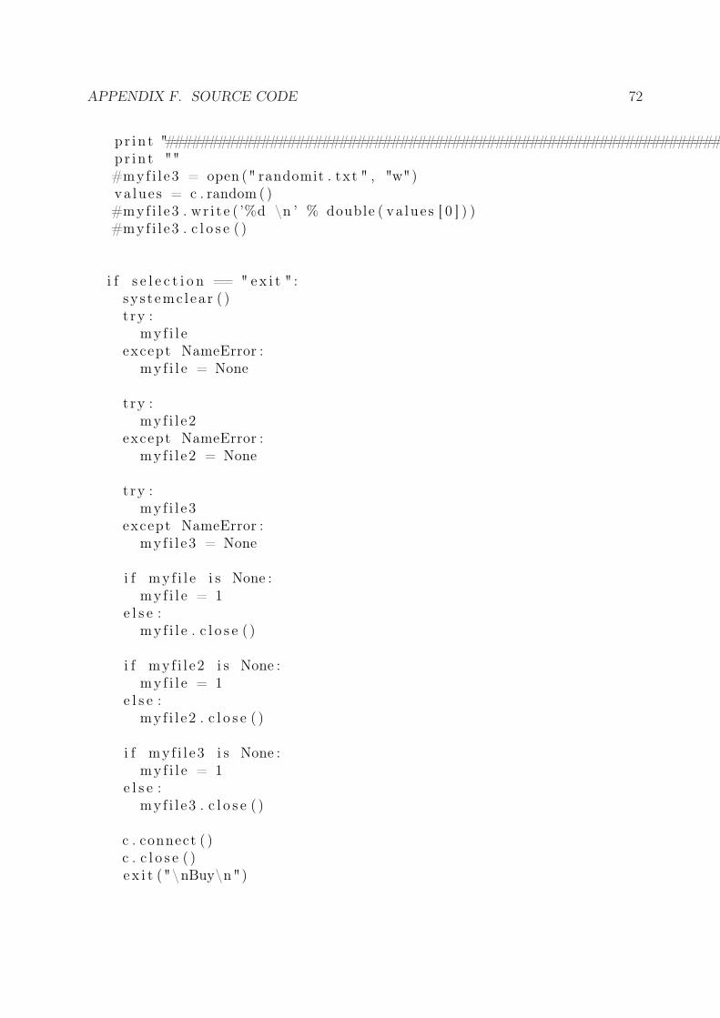
APPENDIX F. SOURCE CODE 72
p r i n t "########################################################################"pr in t ""#myf i l e3 = open (" randomit . txt " , "w")va lue s = c . random ( )#myf i l e3 . wr i t e ( ’%d \n ’ % double ( va lue s [ 0 ] ) )#myf i l e3 . c l o s e ( )
i f s e l e c t i o n == " ex i t " :sy s t emc l ea r ( )t ry :
my f i l eexcept NameError :
my f i l e = None
try :myf i l e2
except NameError :myf i l e2 = None
try :myf i l e3
except NameError :myf i l e3 = None
i f my f i l e i s None :my f i l e = 1
e l s e :my f i l e . c l o s e ( )
i f myf i l e2 i s None :my f i l e = 1
e l s e :my f i l e2 . c l o s e ( )
i f myf i l e3 i s None :my f i l e = 1
e l s e :my f i l e3 . c l o s e ( )
c . connect ( )c . c l o s e ( )e x i t ("\nBuy\n")
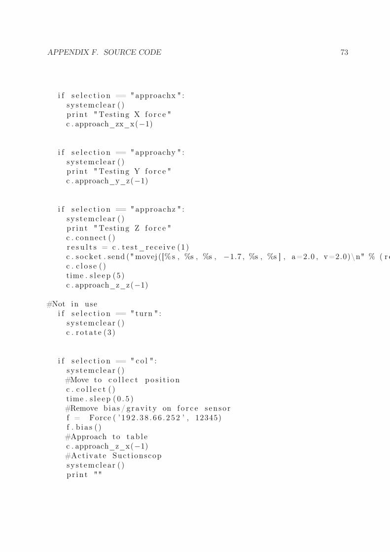
APPENDIX F. SOURCE CODE 73
i f s e l e c t i o n == "approachx " :sy s t emc l ea r ( )p r i n t "Test ing X f o r c e "c . approach_zx_x(−1)
i f s e l e c t i o n == "approachy " :sy s t emc l ea r ( )p r i n t "Test ing Y f o r c e "c . approach_y_z(−1)
i f s e l e c t i o n == "approachz " :sy s t emc l ea r ( )p r i n t "Test ing Z f o r c e "c . connect ( )r e s u l t s = c . t e s t_r e c e i v e (1 )c . socke t . send ("movej ([%s , %s , %s , −1.7 , %s , %s ] , a=2.0 , v=2.0)\n" % ( r e s u l t s . va lue s [ 3 0 ] , r e s u l t s . va lue s [ 3 1 ] , r e s u l t s . va lue s [ 3 2 ] , r e s u l t s . va lue s [ 3 4 ] , r e s u l t s . va lue s [ 3 5 ] ) )c . c l o s e ( )time . s l e e p (5 )c . approach_z_z(−1)
#Not in usei f s e l e c t i o n == " turn " :
sy s t emc l ea r ( )c . r o t a t e (3 )
i f s e l e c t i o n == " co l " :sy s t emc l ea r ( )#Move to c o l l e c t p o s i t i o nc . c o l l e c t ( )time . s l e e p ( 0 . 5 )#Remove b ia s / g rav i ty on f o r c e s enso rf = Force ( ’ 1 9 2 . 3 8 . 6 6 . 2 5 2 ’ , 12345)f . b i a s ( )#Approach to tab l ec . approach_z_x(−1)#Act ivate Suct ionscopsys t emc l ea r ( )p r i n t ""

APPENDIX F. SOURCE CODE 74
p r i n t "######################"pr in t "### Secur ing p l a t e ###"pr in t "######################"pr in t ""time . s l e e p (3 )
i f s e l e c t i o n == " de l " :whi l e ( 1 ) :
sy s t emc l ea r ( )#Move to c o l l e c t p o s i t i o nc . d e l i v e r ( )time . s l e e p ( 0 . 2 )#Remove b ia s / g rav i ty on f o r c e s enso rf = Force ( ’ 1 9 2 . 3 8 . 6 6 . 2 5 2 ’ , 12345)f . b i a s ( )#Approach to tab l ec . approach_z_x(−1)#Deact ivate Suct ionscopsys t emc l ea r ( )
i f s e l e c t i o n == "deburr " :sy s t emc l ea r ( )p r i n t "Moving robot in to s t a r t po s i t i on , p l e a s e wait "c . i n i t i a l i z e ( )sy s t emc l ea r ( )f = Force ( ’ 1 9 2 . 3 8 . 6 6 . 2 5 2 ’ , 12345)f . b i a s ( )c . i n i t_va r i a b l e s ( 4 , 0 . 0 2 , 0 . 0 005 , 1 )p l a t e s = 1p l a t e s = raw_input ("How many p l a t e s should be deburred ? (MAX 10 ) : ")t ry :
p l a t e s = f l o a t ( p l a t e s )except Exception , e :
p r i n t "Error ! " , e , " Please make sure you put in a number between 1−10"e x i t ("\nTry s t a r t i n g the program again \n")
i f p l a t e s > 10 :p r i n t ""p r i n t "#################################"pr in t "### Deburring p l a t e s 10 ###"pr in t "#################################"pr in t ""

APPENDIX F. SOURCE CODE 75
p l a t e s = 10e l i f p l a t e s <= 0 :
p r i n t ""p r i n t "#################################"pr in t "### NOT Deburring any p l a t e s ###"pr in t "#################################"pr in t ""time . s l e e p (3 )
deburred_plates = 0sys t emc l ea r ( )whi l e deburred_plates < p l a t e s :
p r i n t ""p r i n t "#################################"pr in t "### Plate no %s i s running ###" % s t r ( deburred_plates+1)p r i n t "#################################"pr in t ""turncounter = 0c . c o l l e c t ( turncounter )c . deburr ( turncounter )c . d e l i v e r ( )deburred_plates = deburred_plates + 1
c . i n i t i a l i z e ( )sy s t emc l ea r ( )p r i n t ""p r i n t "##################################"pr in t "### Fini shed deburr ing p l a t e s ###"pr in t "##################################"pr in t ""
#In use ?i f s e l e c t i o n == "deburrpos " :
sy s t emc l ea r ( )c . move_to_deburr_pos ( )time . s l e e p (5 )
#In use ?i f s e l e c t i o n == " too lend " :
c . connect ( )r e s u l t s = c . t e s t_r e c e i v e (1 )p r i n t r e s u l t s . va lue s [ 3 5 ]time . s l e e p (5 )
s e l e c t i o n = ""

APPENDIX F. SOURCE CODE 76
F.0.2 connectionregulatortest.py
# TCP c l i e n timport numpyfrom numpy import ∗import socke tsocke t . s e td e f au l t t imeou t ( 1 . 0 )#from time import c lock , timefrom time import ∗#import timeimport timeimport l o c a l el o c a l e . s e t l o c a l e ( l o c a l e .LC_NUMERIC, ’ ’ )import s t r u c tfrom f o r c e import Forceimport l o c a l el o c a l e . s e t l o c a l e ( l o c a l e .LC_NUMERIC, ’ ’ )
c l a s s Connection :de f __init__( s e l f , ip , port ) : #I n i t o f the Connection program , By Orn & Ein i r
s e l f . ip = ips e l f . port = port
de f connect ( s e l f ) : #Connector , Part ly by Orn & Ein i rs e l f . s ocke t = socket . socke t ( socke t .AF_INET, socket .SOCK_STREAM)try :
data2 = s e l f . s ocke t . connect ( ( s e l f . ip , s e l f . port ) )except Exception , e :
p r i n t "Error ! Socket e r r o r was : " , e , " Remember to e s t a b l i s h connect ion to the robot phys i ca ly "e x i t ("\nBuy\n")
s e l f . s ocke t . s e t t imeout ( 1 . 0 )
de f e s tab l i sh_connec t i on ( s e l f ) : #Es tab l i sh the connect ion , By Orn & Ein i rs e l f . connect ( )
de f t e s t_r e c e i v e ( s e l f , n ) : #Function that reads the socket stream and re tu rn s p o s i t i o n data from the robot , By Orn & Ein i rf o r i in range (n ) :
t ry :data = s e l f . read_socket_stream ( )
except Exception , e :p r i n t i , "Error ! " , e , " t ry ing to reconnect "s e l f . e s tab l i sh_connec t i on ( )
re turn data

APPENDIX F. SOURCE CODE 77
de f t e s t_re c e i v e2 ( s e l f , n , f o r c e ) : #Function that takes f o r c e vec to r as input and reads the socke t stream and re tu rn s p o s i t i o n data and f o r c e data ( in robot coo rd inate system ) , By Orn & Ein i rf o r i in range (n ) :
t ry :data = s e l f . read_socket_stream ( )p = s e l f . forward_kin ( data . va lue s [ 3 0 ] , data . va lue s [ 3 1 ] , data . va lue s [ 3 2 ] , data . va lue s [ 3 3 ] , data . va lue s [ 3 4 ] , data . va lue s [ 3 5 ] )f = s e l f . f o r c e_ro ta t i on ( data . va lue s [ 3 0 ] , data . va lue s [ 3 1 ] , data . va lue s [ 3 2 ] , data . va lue s [ 3 3 ] , data . va lue s [ 3 4 ] , data . va lue s [ 3 5 ] , f o r c e )
except Exception , e :p r i n t i , "Error ! " , e , " t ry ing to reconnect "s e l f . e s tab l i sh_connec t i on ( )
#f = [0 0 0 ]re turn array ( [ [ p , f ] ] )
de f read_socket_stream ( s e l f ) : #Function that conver t s the bytestream , from the robot , to usab le data , By Orn & Ein i rmsg_size , time = s t r u c t . unpack( ’> id ’ , s e l f . s ocke t . recv (12 ) ) #4( i n t ) + 8( double )msg_size = msg_size − 12data = s e l f . s ocke t . recv (msg_size )va lue s = s t r u c t . unpack(’>%dd’%(msg_size /8) , data )re turn Resu l t s ( time , va lue s )
de f i n i t i a l i z e ( s e l f ) : #Moves the robot to s t a r t po s i t i on , Part ly by Orn & Ein i rs e l f . connect ( )
# pos = [0 . 000000 , −1.553417118727561 , −1.5863126739797573 , −0.03694351868009342 , 1 .57079632686574611 , 0 . 0 1 ]pos = [0 . 000000 , −1.553417118727561 , −1.5863126739797573 , −0.03694351868009342 , 1 .57079632686574611 , 0 . 0000000 ]pos1 = [ 0 . 0 0 , −1.55 , −1.58 , −0.03 , 1 . 57 , 0 . 0 1 ]s e l f . s ocke t . send ("movej(%s , a=1.0 , v=0.31975511965976)\n" % pos )
# s e l f . s ocke t . send ("movej ( [−0.001279959781185732 , −1.553417118727561 , −1.5863126739797573 , −0.03694351868009342 , 1 .4495583578125688 , 0 . 0 ] , a=1.0 , v=0.31975511965976)\n")i=0whi l e ( i < 5 ) : #While loop , which c on t r o l s that the robot have moved in to the r i g t h pos i t i on , b e f o r e moving on
r e s u l t s = s e l f . read_socket_stream ( )i f r e s u l t s . va lue s [ i +30] <= pos [ i ]+0.001 and r e s u l t s . va lue s [ i +30] >= pos [ i ] −0.001 :
i = i + 1#pr in t "%s" % ( i )
s e l f . s ocke t . c l o s e ( )
de f i n i t_va r i a b l e s ( s e l f , Fref , speed , kp , l agbust ) : #Sets a l l g l oba l cons tant s and the payload o f the robot , Part ly by Orn & Ein i rg l oba l approach_speedg l oba l GFrefg l oba l Kpfg l oba l co s tg l oba l cost_counterg l oba l l a gbu s t e rg l oba l Kpf_matrix
APPENDIX F. SOURCE CODE 78
approach_speed = f l o a t ( speed )GFref = f l o a t ( Fre f )Kpf = f l o a t ( kp )co s t = ze ro s ( ( 1 , 1 5 ) )cost_counter = 0Kpf_matrix = ze ro s ( ( 1 , 1 5 ) )Kpf_counter = 0Way = 0lagbus t e r = in t ( l agbus t )s e l f . connect ( )s e l f . s ocke t . send (" set_payload ( 0 . 5 ) " )s e l f . s ocke t . c l o s e ( )
de f f o r c e_ro ta t i on ( s e l f , t1 , t2 , t3 , t4 , t5 , t6 , Fo ) : #Convert f o r c e data from f o r c e s enso r coo rd ina te system to robot coord ina te system , By Orn & Ein i ra2 = −0.425a3 = −0.39243d1 = 0.0892d4 = 0.109d5 = 0.093d6 = 0.082T01 = array ( [ [ cos ( t1 ) , 0 , s i n ( t1 ) , 0 ] , [ s i n ( t1 ) ,0 ,− cos ( t1 ) , 0 ] , [ 0 , 1 , 0 , d1 ] , [ 0 , 0 , 0 , 1 ] ] )T12 = array ( [ [ cos ( t2 ) ,− s i n ( t2 ) , 0 , a2∗ cos ( t2 ) ] , [ s i n ( t2 ) , cos ( t2 ) , 0 , a2∗ s i n ( t2 ) ] , [ 0 , 0 , 1 , 0 ] , [ 0 , 0 , 0 , 1 ] ] )T23 = array ( [ [ cos ( t3 ) ,− s i n ( t3 ) , 0 , a3∗ cos ( t3 ) ] , [ s i n ( t3 ) , cos ( t3 ) , 0 , a3∗ s i n ( t3 ) ] , [ 0 , 0 , 1 , 0 ] , [ 0 , 0 , 0 , 1 ] ] )T34 = array ( [ [ cos ( t4 ) , 0 , s i n ( t4 ) , 0 ] , [ s i n ( t4 ) ,0 ,− cos ( t4 ) , 0 ] , [ 0 , 1 , 0 , d4 ] , [ 0 , 0 , 0 , 1 ] ] )T45 = array ( [ [ cos ( t5 ) ,0 ,− s i n ( t5 ) , 0 ] , [ s i n ( t5 ) , 0 , cos ( t5 ) , 0 ] , [ 0 , −1 ,0 , d5 ] , [ 0 , 0 , 0 , 1 ] ] )T56 = array ( [ [ cos ( t6 ) ,− s i n ( t6 ) , 0 , 0 ] , [ s i n ( t6 ) , cos ( t6 ) , 0 , 0 ] , [ 0 , 0 , 1 , d6 ] , [ 0 , 0 , 0 , 1 ] ] )T06 = dot (T01 , dot (T12 , dot (T23 , dot (T34 , dot (T45 , T56 ) ) ) ) )
R = ze ro s ( ( 3 , 3 ) )R[ 0 , 0 ] = T06 [ 0 , 0 ]R[ 0 , 1 ] = T06 [ 0 , 1 ]R[ 0 , 2 ] = T06 [ 0 , 2 ]R[ 1 , 0 ] = T06 [ 1 , 0 ]R[ 1 , 1 ] = T06 [ 1 , 1 ]R[ 1 , 2 ] = T06 [ 1 , 2 ]R[ 2 , 0 ] = T06 [ 2 , 0 ]R[ 2 , 1 ] = T06 [ 2 , 1 ]R[ 2 , 2 ] = T06 [ 2 , 2 ]
F = ze ro s ( ( 3 , 1 ) )F [ 0 , 0 ] = Fo [ 0 ]F [ 1 , 0 ] = Fo [ 1 ]F [ 2 , 0 ] = Fo [ 2 ]

APPENDIX F. SOURCE CODE 79
K = dot (R,F)K[ 2 , 0 ] = K[2 ,0 ]∗ ( −1) # because o f 180 degree d i f f e r e n c e between Z axes o f wr i s t 3 and f o r c e s enso rre turn K
def send_speed_to_socket ( s e l f , Xspeed , Yspeed , Zspeed , time ) : #Sends speed l commands to the robot , By Orn & Ein i rs e l f . s ocke t . send (" speed l ([% f , %f , %f , 0 . 0 , 0 . 0 , 0 .0 ] , 1 ,% f )\n" % (Xspeed , Yspeed , Zspeed , 0 . 1 ) )
de f send_cartes ian_to_socket ( s e l f , Xpos , Ypos , Zpos ) : #Sends cood inate s to the robot , us ing the movel command , By Orn & Ein i rs e l f . connect ( )s e l f . s ocke t . send ("movel (p[%f , %f , %f , 0 . 0 , 1 . 57 , 0 ] , a=0.01 ,v=0.01 , t=10)\n" % (Xpos , Ypos , Zpos ) )s e l f . s ocke t . c l o s e ( )
de f polynomial ( s e l f , begin , end , t f ) : #Cubic polynomial , By Orn & Ein i ri f t f < 0 . 1 :
t f = 0 .1r e s = 125 . / 3 . #Reso lut ion : the ra t e that we send commands to the robot o r i g i n a l 1 25 . / 3 .t = arange (0 , t f , 1 / ( f l o a t ( r e s ) ) ) #Make a time vec to ra0 = begina2 = 3 ./ t f ∗∗2∗( end−begin )a3 = −2./ t f ∗∗3∗( end−begin )p o s i t i o n = ze ro s ( ( 1 , l en ( t ) ) )speed = ze ro s ( ( 1 , l en ( t ) ) )f o r i in range ( l en ( t ) ) :
p o s i t i o n [ ( 0 , i ) ] = a0 + a2∗ t [ i ]∗∗2 + a3∗ t [ i ]∗∗3speed [ ( 0 , i ) ] = 2 ∗ a2 ∗ t [ i ] + 3 ∗ a3 ∗ t [ i ]∗∗2
re turn [ po s i t i on , speed ]
de f polynomial2 ( s e l f , begin , end , t f , r e s o l u t i o n ) : #Cubic polynomial , takes more inputs , By Orn & Ein i ri f t f < 0 . 1 :
t f = 0 .1r e s = f l o a t ( r e s o l u t i o n ) #Reso lut ion : the ra t e that we send commands to the robott = arange (0 , t f , 1 / ( f l o a t ( r e s ) ) ) #Make a time vec to ra0 = begina2 = 3 ./ t f ∗∗2∗( end−begin )a3 = −2./ t f ∗∗3∗( end−begin )p o s i t i o n = ze ro s ( ( 1 , l en ( t ) ) )speed = ze ro s ( ( 1 , l en ( t ) ) )f o r i in range ( l en ( t ) ) :
p o s i t i o n [ ( 0 , i ) ] = a0 + a2∗ t [ i ]∗∗2 + a3∗ t [ i ]∗∗3speed [ ( 0 , i ) ] = 2 ∗ a2 ∗ t [ i ] + 3 ∗ a3 ∗ t [ i ]∗∗2
re turn [ po s i t i on , speed ]

APPENDIX F. SOURCE CODE 80
de f ca l cu late_t ime ( s e l f , beginX , beginY , beginZ , endX , endY , endZ ) : #Function that c a l c u l a t e s the amount o f time needed f o r a movement , By Orn & Ein i rt f = ( sq r t ( ( beginX−endX)∗∗2+(beginY−endY)∗∗2+(beginZ−endZ )∗∗2 ) ) /0 . 05re turn t f
de f t r a n s l a t e ( s e l f , Xend , Yend , Zend , Fref , turncounter , Freg , r e s ) : #Function that can make a 3−dimens iona l movement with the robot , Part ly Orn & Ein i rs e l f . connect ( )r e s u l t s = s e l f . t e s t_r e c e i v e (1 )f = s e l f . forward_kin ( r e s u l t s . va lue s [ 3 0 ] , r e s u l t s . va lue s [ 3 1 ] , r e s u l t s . va lue s [ 3 2 ] , r e s u l t s . va lue s [ 3 3 ] , r e s u l t s . va lue s [ 3 4 ] , r e s u l t s . va lue s [ 3 5 ] )regu latorbreytaX = f [ 0 ]regu latorbreytaY = f [ 1 ]r egu la to rbrey taZ = f [ 2 ]s e l f . c l o s e ( )
T = s e l f . ca l cu late_t ime (0 , 0 , 0 ,Xend , Yend , Zend )
k1 = s e l f . polynomial2 (0 ,Xend ,T, r e s )k2 = s e l f . polynomial2 (0 ,Yend ,T, r e s )k3 = s e l f . polynomial2 (0 , Zend ,T, r e s )K = [ k1 [0 ]+ regulatorbreytaX , k2 [0 ]+ regulatorbreytaY , k3 [0 ]+ regu latorbreytaZ , k1 [ 1 ] , k2 [ 1 ] , k3 [ 1 ] ]s e l f . draw (K, Fref , turncounter , Freg )
de f draw ( s e l f , k , Fref , turncounter , Freg ) : #Important func t i on : Works as p o s i t i o n and f o r c e c o n t r o l l e r whi l e sending speed commands to the robot , Part ly Orn & Ein i r#The func t i on a l s o wr i t e s p o s i t i o n and f o r c e data to a f i l e f o r f u r t h e r a n a l y s i s .Xp=k [ 0 ] #X po s i t i o nYp=k [ 1 ] #Y po s i t i o nZp=k [ 2 ] #Z po s i t i o nXd=k [ 3 ] #X speedYd=k [ 4 ] #Y speedZd=k [ 5 ] #Z speed#myf i l e = open ("draw . txt " , "a ")
#I n i t i a l i z e v a r i a b l e scor rec t ionX = 0cor rec t ionY = 0co r r e c t i onZ = 0integratorX = 0integratorY = 0in t eg ra to rZ = 0co r r e c t i o n = 0integ ra to rFx = 0 #added f o r r e gu l a t i o n on p l a t e sin t eg ra to rFy = 0 #added f o r r e gu l a t i o n on p l a t e si n t eg ra to rFz = 0 #Orns o r i g i n a l r e gu l a t i o n
APPENDIX F. SOURCE CODE 81
g l oba l GFrefFre f = GFrefg l oba l l a gbu s t e r #I f l a gbu s t e r i s on , then the program w i l l c l e a r the socke t queue i f l ag i s detec ted
################################################################ Regulat ion in s enso r Z−ax i s ##################################################################
counter = 1i=0s e l f . connect ( )my f i l e = open (" t e s t i t . txt " , "a ")f o = Force ( ’ 1 9 2 . 3 8 . 6 6 . 2 5 2 ’ , 12345)fo . e s tab l i sh_connec t i on ( )g l oba l Kpff o r j in range (Xd. shape [ 1 ] ∗ 3 ) :
r e s u l t s = s e l f . t e s t_r e c e i v e (1 )i f counter == 3 : #Sending commands at 41 .6Hz , 125Hz/3
time1 = c lock ( )# pr in t "####moving####"
s e l f . send_speed_to_socket (Xd[ ( 0 , i )]+ correct ionX ,Yd[ ( 0 , i )]+ correct ionY , Zd [ ( 0 , i )]+ cor rec t i onZ , 0 . 0 1 )f o . send_to_socket ( )f o r c e = fo . read_socket_stream ( )myf i l e4 = open ("draw . txt " , "a ")myf i l e4 . wr i t e ( ’% f %f %f %f %f %f %f \n ’ % (Xd[ ( 0 , i ) ] , correct ionX ,Yd[ ( 0 , i ) ] , correct ionY , Zd [ ( 0 , i ) ] , co r r ec t i onZ , f o r c e [ 2 ] ) )myf i l e4 . c l o s e ( )f = s e l f . forward_kin ( r e s u l t s . va lue s [ 3 0 ] , r e s u l t s . va lue s [ 3 1 ] , r e s u l t s . va lue s [ 3 2 ] , r e s u l t s . va lue s [ 3 3 ] , r e s u l t s . va lue s [ 3 4 ] , r e s u l t s . va lue s [ 3 5 ] )
###Error and In t e g r a t i on###errorX = Xp[ ( 0 , i )]− f [ 0 ]errorY = Yp[ ( 0 , i )]− f [ 1 ]e r rorZ = Zp [ ( 0 , i )]− f [ 2 ]in tegratorX = integratorX + errorXintegratorY = integratorY + errorYin t eg ra to rZ = in t eg ra to rZ + errorZ
errorFz = Fre f − f o r c e [ 2 ]
#########Correc t i on s##############Force PI Regulator###int eg ra to rFz = in t eg ra to rFz + errorFzKif = 0.0005/20

APPENDIX F. SOURCE CODE 82
cor rec t ionX = Kpf∗ er rorFz + Kif ∗ i n t eg ra to rFz
###Pos i t i on PI Regulator###Kp = 5Ki = 0.05cor rec t ionY = Kp∗ errorY + Ki∗ i n tegratorYco r r e c t i onZ = Kp∗ er rorZ + Ki∗ i n t eg ra to rZ
i f Freg == 0 :cor rec t ionX = 0cor rec t ionY = 0co r r e c t i onZ = 0
#Write po s i t i on , speed , c on t r o l s i g n a l and f o r c e data to a f i l emy f i l e . wr i t e ( ’% f %f %f %f %f %f %f %f %f %f \n ’ % (Xd[ ( 0 , i ) ] ,Yd [ ( 0 , i ) ] , Zd [ ( 0 , i ) ] , f [ 0 ] , f [ 1 ] , f [ 2 ] ,Xp[ ( 0 , i ) ] ,Yp [ ( 0 , i ) ] , Zp [ ( 0 , i ) ] , f o r c e [ 2 ] ) )
counter = 0 ;i=i +1;time2 = c lock ( )#This r ou t in e c l e a r s the socke t bu f f e r i f l ag i s detec tedi f l a gbu s t e r == 1 :
i f time2−time1 > 0 . 1 :p r i n t "########Lag detec ted######## Clear ing %i socke t packets " % in t ( f l o o r (125∗ ( time2−time1 ) ) )f o r count in range (1 , 5+in t ( f l o o r (125∗ ( time2−time1 ) ) ) ) :
s e l f . t e s t_r e c e i v e (1 )counter = counter + 1 ;
s e l f . c l o s e ( )
de f forward_kin ( s e l f , t1 , t2 , t3 , t4 , t5 , t6 ) : #Ca lcu la te forward k inemat i c s by us ing j o i n t p o s i t i o n s from robot , By Orn & Ein i ra2 = −0.425a3 = −0.39243d1 = 0.0892d4 = 0.109d5 = 0.093d6 = 0.082T01 = array ( [ [ cos ( t1 ) , 0 , s i n ( t1 ) , 0 ] , [ s i n ( t1 ) ,0 ,− cos ( t1 ) , 0 ] , [ 0 , 1 , 0 , d1 ] , [ 0 , 0 , 0 , 1 ] ] )T12 = array ( [ [ cos ( t2 ) ,− s i n ( t2 ) , 0 , a2∗ cos ( t2 ) ] , [ s i n ( t2 ) , cos ( t2 ) , 0 , a2∗ s i n ( t2 ) ] , [ 0 , 0 , 1 , 0 ] , [ 0 , 0 , 0 , 1 ] ] )T23 = array ( [ [ cos ( t3 ) ,− s i n ( t3 ) , 0 , a3∗ cos ( t3 ) ] , [ s i n ( t3 ) , cos ( t3 ) , 0 , a3∗ s i n ( t3 ) ] , [ 0 , 0 , 1 , 0 ] , [ 0 , 0 , 0 , 1 ] ] )T34 = array ( [ [ cos ( t4 ) , 0 , s i n ( t4 ) , 0 ] , [ s i n ( t4 ) ,0 ,− cos ( t4 ) , 0 ] , [ 0 , 1 , 0 , d4 ] , [ 0 , 0 , 0 , 1 ] ] )T45 = array ( [ [ cos ( t5 ) ,0 ,− s i n ( t5 ) , 0 ] , [ s i n ( t5 ) , 0 , cos ( t5 ) , 0 ] , [ 0 , −1 ,0 , d5 ] , [ 0 , 0 , 0 , 1 ] ] )T56 = array ( [ [ cos ( t6 ) ,− s i n ( t6 ) , 0 , 0 ] , [ s i n ( t6 ) , cos ( t6 ) , 0 , 0 ] , [ 0 , 0 , 1 , d6 ] , [ 0 , 0 , 0 , 1 ] ] )T06 = dot (T01 , dot (T12 , dot (T23 , dot (T34 , dot (T45 , T56 ) ) ) ) )x = T06 [0 ,3 ]+0 .0606

APPENDIX F. SOURCE CODE 83
y = T06 [ 1 , 3 ]z = T06 [ 2 , 3 ]r e turn [ x , y , z ]
de f approach ( s e l f ) : #Moves the robot near the blackboard , By Orn & Ein i rs e l f . connect ( )f o = Force ( ’ 1 9 2 . 3 8 . 6 6 . 2 5 2 ’ , 12345)fo . e s tab l i sh_connec t i on ( )counter = 0whi l e ( 1 ) :
counter = counter + 1r e s u l t s = s e l f . t e s t_r e c e i v e (1 )i f counter == 3 : #Sending commands at 41Hz , 125Hz/3
fo . send_to_socket ( )f o r c e = fo . read_socket_stream ( )i f f o r c e [ 2 ] < 0 . 4 :
s e l f . send_speed_to_socket ( approach_speed , 0 . 0 , 0 . 0 , 0 . 0 4 )e l s e :
s e l f . send_speed_to_socket ( 0 . 0 , 0 . 0 , 0 . 0 , 0 . 0 4 )s e l f . c l o s e ( )break
counter = 0
de f wr i t e_to_f i l e ( s e l f , matrix ) : #Writes out data in to a f i l e , By Orn & Ein i rmy f i l e = open (" output . txt " , "w")f o r i in range ( matrix . shape [ 1 ] ) :
my f i l e . wr i t e ( ’% f \n ’ % ( matrix [ ( 0 , i ) ] ) )
de f p o s i t i o n ( s e l f ) : #Reads out the po s i t i o n o f the robot , By Orn & Ein i rs e l f . e s tab l i sh_connec t i on ( )r e s u l t s = s e l f . read_socket_stream ( )pos = s e l f . forward_kin ( r e s u l t s . va lue s [ 3 0 ] , r e s u l t s . va lue s [ 3 1 ] , r e s u l t s . va lue s [ 3 2 ] , r e s u l t s . va lue s [ 3 3 ] , r e s u l t s . va lue s [ 3 4 ] , r e s u l t s . va lue s [ 3 5 ] )s e l f . c l o s e ( )re turn pos
de f __del__( s e l f ) : #Fundamental func t i on in Python , Cal led when the in s t anc e i s about to be destroyeds e l f . c l o s e ( )
de f c l o s e ( s e l f ) : #Close down every socke t connect ioni f s e l f . s ocke t :
s e l f . s ocke t . c l o s e ( )
de f random( s e l f ) : #Function to t e s t send and r e c e i v e speed from robot

APPENDIX F. SOURCE CODE 84
t = 0myf i l e3 = open (" randomit . txt " , "a ")whi l e t <5:
s e l f . connect ( )s2 = s e l f . s ocke t . send (" random ( ) " )s = s e l f . read_random ( )myf i l e3 . wr i t e ( ’ S2 : %s S : %s t : %f \n ’ % ( s2 , s , t ) )t = t + 1s e l f . s ocke t . c l o s e ( )
myf i l e3 . c l o s e ( )re turn s
de f read_random( s e l f ) : #Function to read out the returned msg from robot when random i s c a l l e dmsg_size , time = s t r u c t . unpack( ’> id ’ , s e l f . s ocke t . recv (12 ) ) #4( i n t ) + 8( double )msg_size = msg_size − 12data = s e l f . s ocke t . recv (msg_size )va lue s = s t r u c t . unpack(’>%dd ’ % (msg_size /8) , data )va lues2 = array ( [ [ s t r ( va lue s [ 5 5 ] ) ] , [ s t r ( va lue s [ 5 6 ] ) ] ] )my f i l e = open (" data . txt " , "a ")t = 0whi l e t < 11 :
my f i l e . wr i t e ( ’ va lue 40 indeho lde r %s\n ’ % ( va lue s [ 4 0 ] ) )my f i l e . wr i t e ( ’ va lue 55 indeho lde r %s\n ’ % ( va lue s [ 5 5 ] ) )my f i l e . wr i t e ( ’ va lue 56 indeho lde r %s\n ’ % ( va lue s [ 5 6 ] ) )my f i l e . wr i t e ( ’ va lue 60 indeho lde r %s\n ’ % ( va lue s [ 6 0 ] ) )t = t+1
myf i l e . c l o s e ( )re turn [ va lues2 [ 0 ] , va lues2 [ 1 ] ]
de f approach_z_x ( s e l f , d i r e c t i o n ) : #When the x d i r e c t i o n o f the s enso r are in the z d i r e c t i o n o f the robots e l f . connect ( )f o = Force ( ’ 1 9 2 . 3 8 . 6 6 . 2 5 2 ’ , 12345)fo . e s tab l i sh_connec t i on ( )counter = 0i = 0whi l e ( 1 ) :
i = i+1counter = counter + 1r e s u l t s = s e l f . t e s t_r e c e i v e (1 )i f counter == 10 : #Sending commands at 41Hz , 125Hz/3
fo . send_to_socket ( )f o r c e = fo . read_socket_stream ( )i f f o r c e [ 2 ] > −3.0 and f o r c e [ 2 ] < 3 . 0 :

APPENDIX F. SOURCE CODE 85
i f d i r e c t i o n == −1:s e l f . send_speed_to_socket (0 .0 ,0 .0 , − approach_speed , 0 . 0 4 ) #Moves the robot in i t s Z−plane in a negat ive d i r e c t i o n
e l i f d i r e c t i o n == 1 :s e l f . send_speed_to_socket ( 0 . 0 , 0 . 0 , approach_speed , 0 . 0 4 ) #Moves the robot in i t s Z−plane in a p o s i t i v e d i r e c t i o n
e l i f f o r c e [ 2 ] > 3 . 0 :s e l f . send_speed_to_socket ( 0 . 0 , 0 . 0 , 0 . 0 , 0 . 0 4 )s e l f . c l o s e ( )break
e l i f f o r c e [ 2 ] < −3.0:s e l f . send_speed_to_socket ( 0 . 0 , 0 . 0 , 0 . 0 , 0 . 0 4 )s e l f . c l o s e ( )break
e l s e :s e l f . send_speed_to_socket ( 0 . 0 , 0 . 0 , 0 . 0 , 0 . 0 4 )s e l f . c l o s e ( )break
counter = 0
de f approach_zx_x ( s e l f , z d i r e c t i on , xd i r e c t i on , f , r e f ) : #When the x d i r e c t i o n o f the s enso r are in the zANDx d i r e c t i o n o f the robots e l f . connect ( )f o = Force ( ’ 1 9 2 . 3 8 . 6 6 . 2 5 2 ’ , 12345)fo . e s tab l i sh_connec t i on ( )counter = 0i = 0whi l e ( 1 ) :
i = i+1counter = counter + 1r e s u l t s = s e l f . t e s t_r e c e i v e (1 )i f counter == 10 : #Sending commands at 41Hz , 125Hz/3
fo . send_to_socket ( )f o r c e = fo . read_socket_stream ( )i f f o r c e [ f ] > −r e f and f o r c e [ f ] < r e f :
i f z d i r e c t i o n == −1:i f x d i r e c t i o n == −1:
s e l f . send_speed_to_socket(−approach_speed /4 ,0.0 ,− approach_speed /4 , 0 . 04 ) #Moves the robot in i t s ZandX−plane in a negat ive d i r e c t i o ne l i f x d i r e c t i o n == 1 :
s e l f . send_speed_to_socket ( approach_speed /4 ,0.0 ,− approach_speed /4 , 0 . 04 ) #Moves the robot in i t s ZandX−plane in a negat ive d i r e c t i o ne l i f z d i r e c t i o n == 1 :
i f x d i r e c t i o n == −1:s e l f . send_speed_to_socket(−approach_speed /4 , 0 . 0 , approach_speed /4 , 0 . 04 ) #Moves the robot in i t s ZandX−plane in a negat ive d i r e c t i o n
e l i f x d i r e c t i o n == 1 :s e l f . send_speed_to_socket ( approach_speed /4 , 0 . 0 , approach_speed /4 , 0 . 04 ) #Moves the robot in i t s ZandX−plane in a negat ive d i r e c t i o n
e l i f f o r c e [ f ] > r e f :

APPENDIX F. SOURCE CODE 86
s e l f . send_speed_to_socket ( 0 . 0 , 0 . 0 , 0 . 0 , 0 . 0 4 )s e l f . c l o s e ( )break
e l i f f o r c e [ f ] < −r e f :s e l f . send_speed_to_socket ( 0 . 0 , 0 . 0 , 0 . 0 , 0 . 0 4 )s e l f . c l o s e ( )break
e l s e :s e l f . send_speed_to_socket ( 0 . 0 , 0 . 0 , 0 . 0 , 0 . 0 4 )s e l f . c l o s e ( )break
counter = 0
de f decouple ( s e l f , plane , d i s tance , turncounter ) : #Function which moves the robot a d i s t ance (m) away in the X−, Y−, or Z−plane , takes a s t r i n g and two f l o a t s as inputi f p lane == "x" or plane == "X" :
s e l f . t r a n s l a t e ( d i s tance , 0 . 0 , 0 . 0 , 0 , turncounter , 0 , 1 2 5 . / 3 . )e l i f p lane == "y" or plane == "Y" :
s e l f . t r a n s l a t e ( 0 . 0 , d i s tance , 0 . 0 , 0 , turncounter , 0 , 1 2 5 . / 3 . )e l i f p lane == "z" or plane == "Z" :
s e l f . t r a n s l a t e ( 0 . 0 , 0 . 0 , d i s tance , 0 , turncounter , 0 , 1 2 5 . / 3 . )e l s e :
p r i n t "Error ! The one or both inputs in decouple are wrong"
de f r o t a t e ( s e l f , counter ) : #Function which r o t a t e s the TCP of the robot wihtout g e t t i n g out o f range o f the Wrist 3 and the wi re si f counter == 0 : # Rotate to s t a r t p o s i t i o n (~−0 deg r e s s )
s e l f . connect ( )r e s u l t s = s e l f . t e s t_r e c e i v e (1 )pos = [0 .17551645190320445 ]s e l f . s ocke t . send ("movej ([%s , %s , %s , %s , %s , %s ] , a=2.0 , v=2.0)\n" % ( r e s u l t s . va lue s [ 3 0 ] , r e s u l t s . va lue s [ 3 1 ] , r e s u l t s . va lue s [ 3 2 ] , r e s u l t s . va lue s [ 3 3 ] , r e s u l t s . va lue s [ 3 4 ] , pos [ 0 ] ) )i = 0whi l e ( i <= 0 ) :
r e s u l t s = s e l f . read_socket_stream ( )i f r e s u l t s . va lue s [ 3 5 ] <= pos [0 ]+0 .005 and r e s u l t s . va lue s [ 3 5 ] >= pos [ 0 ] −0 .005 :
f = Force ( ’ 1 9 2 . 3 8 . 6 6 . 2 5 2 ’ , 12345)f . b i a s ( )break
s e l f . s ocke t . c l o s e ( )
e l i f counter == 1 : # Rotate to second po s i t i o n (~−90 deg r e s s )s e l f . connect ( )r e s u l t s = s e l f . t e s t_r e c e i v e (1 )pos = [−1.570796327+0.17551645190320445]s e l f . s ocke t . send ("movej ([%s , %s , %s , %s , %s , %s ] , a=2.0 , v=2.0)\n" % ( r e s u l t s . va lue s [ 3 0 ] , r e s u l t s . va lue s [ 3 1 ] , r e s u l t s . va lue s [ 3 2 ] , r e s u l t s . va lue s [ 3 3 ] , r e s u l t s . va lue s [ 3 4 ] , pos [ 0 ] ) )

APPENDIX F. SOURCE CODE 87
i = 0whi l e ( i == 0 ) :
r e s u l t s = s e l f . read_socket_stream ( )i f r e s u l t s . va lue s [ 3 5 ] <= pos [0 ]+0 .005 and r e s u l t s . va lue s [ 3 5 ] >= pos [ 0 ] −0 .005 :
f = Force ( ’ 1 9 2 . 3 8 . 6 6 . 2 5 2 ’ , 12345)f . b i a s ( )break
s e l f . s ocke t . c l o s e ( )my f i l e = open (" data . txt " , "a ")my f i l e . wr i t e ( ’%s , %s , %s , %s , %s , %s \n ’ % ( r e s u l t s . va lue s [ 3 0 ] , r e s u l t s . va lue s [ 3 1 ] , r e s u l t s . va lue s [ 3 2 ] , r e s u l t s . va lue s [ 3 3 ] , r e s u l t s . va lue s [ 3 4 ] , r e s u l t s . va lue s [ 3 5 ] ) )my f i l e . c l o s e ( )
e l i f counter == 2 : # Rotate to th i rd po s i t i o n (~−135 deg r e s s )s e l f . connect ( )r e s u l t s = s e l f . t e s t_r e c e i v e (1 )pos = [−3.141592654+0.17551645190320445]s e l f . s ocke t . send ("movej ([%s , %s , %s , %s , %s , %s ] , a=2.0 , v=2.0)\n" % ( r e s u l t s . va lue s [ 3 0 ] , r e s u l t s . va lue s [ 3 1 ] , r e s u l t s . va lue s [ 3 2 ] , r e s u l t s . va lue s [ 3 3 ] , r e s u l t s . va lue s [ 3 4 ] , pos [ 0 ] ) )i = 0whi l e ( i == 0 ) :
r e s u l t s = s e l f . read_socket_stream ( )i f r e s u l t s . va lue s [ 3 5 ] <= pos [0 ]+0 .005 and r e s u l t s . va lue s [ 3 5 ] >= pos [ 0 ] −0 .005 :
f = Force ( ’ 1 9 2 . 3 8 . 6 6 . 2 5 2 ’ , 12345)f . b i a s ( )break
s e l f . s ocke t . c l o s e ( )my f i l e = open (" data . txt " , "a ")my f i l e . wr i t e ( ’%s , %s , %s , %s , %s , %s \n ’ % ( r e s u l t s . va lue s [ 3 0 ] , r e s u l t s . va lue s [ 3 1 ] , r e s u l t s . va lue s [ 3 2 ] , r e s u l t s . va lue s [ 3 3 ] , r e s u l t s . va lue s [ 3 4 ] , r e s u l t s . va lue s [ 3 5 ] ) )my f i l e . c l o s e ( )
e l i f counter == 3 : # Rotate to four th po s i t i o n (~−180 deg r e s s )s e l f . connect ( )r e s u l t s = s e l f . t e s t_r e c e i v e (1 )pos = [−4.712388981+0.17551645190320445]s e l f . s ocke t . send ("movej ([%s , %s , %s , %s , %s , %s ] , a=2.0 , v=2.0)\n" % ( r e s u l t s . va lue s [ 3 0 ] , r e s u l t s . va lue s [ 3 1 ] , r e s u l t s . va lue s [ 3 2 ] , r e s u l t s . va lue s [ 3 3 ] , r e s u l t s . va lue s [ 3 4 ] , pos [ 0 ] ) )i = 0whi l e ( i == 0 ) :
r e s u l t s = s e l f . read_socket_stream ( )i f r e s u l t s . va lue s [ 3 5 ] <= pos [0 ]+0 .005 and r e s u l t s . va lue s [ 3 5 ] >= pos [ 0 ] −0 .005 :
f = Force ( ’ 1 9 2 . 3 8 . 6 6 . 2 5 2 ’ , 12345)f . b i a s ( )break
s e l f . s ocke t . c l o s e ( )my f i l e = open (" data . txt " , "a ")

APPENDIX F. SOURCE CODE 88
myf i l e . wr i t e ( ’%s , %s , %s , %s , %s , %s \n ’ % ( r e s u l t s . va lue s [ 3 0 ] , r e s u l t s . va lue s [ 3 1 ] , r e s u l t s . va lue s [ 3 2 ] , r e s u l t s . va lue s [ 3 3 ] , r e s u l t s . va lue s [ 3 4 ] , r e s u l t s . va lue s [ 3 5 ] ) )my f i l e . c l o s e ( )
e l s e :p r i n t "An e r r o r occured in the r o t a t e func t i on "
de f c o l l e c t ( s e l f , turncounter ) : #Make the robot p ick up a p l a t e from a ho lder ( s imulated pick up)s e l f . connect ( )#Move to po s i t i o n f o r c o l l e c t i n g p l a t epos = [−1.26525439665243500 ,−1.44560270287730370 ,−1.68035001330557070 ,−1.59705473420764040 ,1.56520131170505430 ,0.0]s e l f . s ocke t . send ("movej(%s , a=1.0 , v=0.5)\n" % pos )i=0whi l e ( i < 5 ) : #While loop , which c on t r o l s that the robot have moved in to the r i g t h pos i t i on , b e f o r e moving on
r e s u l t s = s e l f . read_socket_stream ( )i f r e s u l t s . va lue s [ i +30] <= pos [ i ]+0.001 and r e s u l t s . va lue s [ i +30] >= pos [ i ] −0.001 :
i = i + 1
s e l f . s ocke t . c l o s e ( )time . s l e e p ( 0 . 5 )#Remove b ia s / g rav i ty on f o r c e s enso rf = Force ( ’ 1 9 2 . 3 8 . 6 6 . 2 5 2 ’ , 12345)f . b i a s ( )#Approach to tab l es e l f . approach_z_x(−1)#Act ivate Suct ionscoppr i n t ""p r i n t "#################################"pr in t "### Secur ing p l a t e ###"pr in t "#################################"pr in t ""time . s l e e p (3 )s e l f . decouple (" z " , 0 . 10 , turncounter )
de f d e l i v e r ( s e l f ) : #Drops o f f the p l a t e in a ho lders e l f . connect ( )#Move to po s i t i o n f o r d e l i v e r i n g p l a t epos = [−0.58933449904424062 ,−2.35443412600472210 ,−0.80623840453672335 ,−1.59831767976512310 ,1.56137153692032670 ,0.0]s e l f . s ocke t . send ("movej(%s , a=1.0 , v=0.5)\n" % pos )i=0whi l e ( i < 5 ) : #While loop , which c on t r o l s that the robot have moved in to the r i g t h pos i t i on , b e f o r e moving onr e s u l t s = s e l f . read_socket_stream ( )i f r e s u l t s . va lue s [ i +30] <= pos [ i ]+0.001 and r e s u l t s . va lue s [ i +30] >= pos [ i ] −0.001 :

APPENDIX F. SOURCE CODE 89
i = i + 1s e l f . s ocke t . c l o s e ( )time . s l e e p ( 0 . 5 )#Remove b ia s / g rav i ty on f o r c e s enso rf = Force ( ’ 1 9 2 . 3 8 . 6 6 . 2 5 2 ’ , 12345)f . b i a s ( )#Approach the tab l es e l f . approach_z_x(−1)#Deact ivate Suct ionscoppr i n t ""p r i n t "#################################"pr in t "### Releas ing p l a t e ###"pr in t "#################################"pr in t ""time . s l e e p (3 )
de f move_to_deburr_pos ( s e l f ) : #Moves the robot to the deburr ing t o o l without turn ing the TCP/Wrist 3s e l f . connect ( )r e s u l t s = s e l f . t e s t_r e c e i v e (1 )po s too l = r e s u l t s . va lue s [ 3 5 ]#Move to po s i t i o n f o r deburr ing the p l a t e
# pos = [0.33146529146213632 ,−2.70883406010032957 ,−0.88330808564727037 ,−0.39678811137280756 ,1.32261049523673324 ,0.17551645190320445]pos = [0.33146529146213632 ,−2.70883406010032957 ,−0.88330808564727037 ,−0.39678811137280756 ,1.32261049523673324 , po s too l ]
# pos = [ 0 . 8 4 4 7 , 0 . 1 5 8 3 , 0 . 0 9 0 0 8 , 0 . 0 , 2 . 3 5 , 0 . 0 ]my f i l e = open (" data . txt " , "a ")my f i l e . wr i t e ("%.17 f ,%.17 f ,%.17 f ,%.17 f ,%.17 f ,%.17 f \n" %(pos [ 0 ] , pos [ 1 ] , pos [ 2 ] , pos [ 3 ] , pos [ 4 ] , pos [ 5 ] ) )my f i l e . c l o s e ( )s e l f . s ocke t . send ("movej(%s , a=1.0 , v=0.5)\n" % pos )
# s e l f . s ocke t . send ("movel (p[%f ,%f ,%f ,%f ,%f ,% f ] , a=1.0 , v=0.5)\n" % ( pos [ 0 ] , pos [ 1 ] , pos [ 2 ] , pos [ 3 ] , pos [ 4 ] , pos [ 5 ] ) )i=0whi l e ( i < 5 ) :
r e s u l t s = s e l f . read_socket_stream ( )i f r e s u l t s . va lue s [ i +30] <= pos [ i ]+0.001 and r e s u l t s . va lue s [ i +30] >= pos [ i ] −0.001 :
i = i + 1s e l f . s ocke t . c l o s e ( )
de f deburr ( s e l f , turncounter ) : #Runs the four s i d e s o f a p l a t e over the deburr ing t o o ls e l f . i n i t i a l i z e ( )p r i n t ""p r i n t "#################################"pr in t "### Deburring p l a t e ###"pr in t "#################################"pr in t ""

APPENDIX F. SOURCE CODE 90
#The deburr ing o f the f i r s t edge s t a r ts e l f . move_to_deburr_pos ( )#Approaching the deburr machinewhi l e turncounter < 4 :
s e l f . r o t a t e (0 ) #Rotates the p l a t e to the f i r s t p o s i t i o ntime . s l e e p ( 0 . 5 ) #The robot has to be complet ly stopped be f o r e removing b ia s#Removes b i a s / g rav i ty from f o r c e s enso rf = Force ( ’ 1 9 2 . 3 8 . 6 6 . 2 5 2 ’ , 12345)f . b i a s ( )
s e l f . approach_zx_x (−1 ,1 ,2 ,4) #Moves the p l a t e aga in s t the deburr ing t o o l to sense were i t i s in the Z d i r e c t i o n o f the s enso rs e l f . t r a n s l a t e ( −0 . 005 , 0 , 0 . 005 , 0 , 0 , 0 , 125 . /3 . ) #Moves a l i t t l e away from the t o o ltime . s l e e p ( 0 . 5 ) #The robot has to be s t i l l b e f o r e removing b ia sf . b i a s ( )s e l f . approach_zx_x(−1 ,−1 ,0 ,5) #Moves the p l a t e aga in s t the deburr ing t o o l to sense were i t i s in the X d i r e c t i o n o f the s enso rtime . s l e e p ( 0 . 5 )
s e l f . approach_zx_x (−1 ,1 ,2 ,4) #Moves the p l a t e back aga in s t the deburr ing t o o ls e l f . t r a n s l a t e ( 0 . 0 , −0 . 2 , 0 . 0 , 5 . 0 , turncounter , 1 , 1 2 5 . 0 ) #Moves the robot s ideways on the deburr ing too l , with r e gu l a t i o n in the Z−d i r e c t i o n o f the s enso rs e l f . decouple ("Z" , 0 . 1 0 , 0 ) #L i f t the robot away from the t o o lturncounter = turncounter + 1i f turncounter < 4 : #Rotates the TCP to the next edge to deburr
s e l f . r o t a t e ( turncounter )e l s e :
s e l f . r o t a t e (0 )
# Comments from edge 1 has to be copied here#The deburr ing o f the second edge s t a r ts e l f . move_to_deburr_pos ( )time . s l e e p ( 0 . 5 )f . b i a s ( )s e l f . approach_zx_x (−1 ,1 ,2 ,4)f . send_to_socket ( )f o r c e = f . read_socket_stream ( )myf i l e1 = open (" f o r c e . txt " , "a ")myf i l e1 . wr i t e ("%f ,%f ,% f \n" %( f o r c e [ 0 ] , f o r c e [ 1 ] , f o r c e [ 2 ] ) )myf i l e1 . c l o s e ( )s e l f . t r a n s l a t e ( −0 . 005 , 0 , 0 . 005 , 0 , 0 , 0 , 125 . /3 . )time . s l e e p ( 0 . 5 )f . b i a s ( )s e l f . approach_zx_x(−1 ,−1 ,1 ,5)f . send_to_socket ( )

APPENDIX F. SOURCE CODE 91
f o r c e = f . read_socket_stream ( )myf i l e1 = open (" f o r c e . txt " , "a ")myf i l e1 . wr i t e ("%f ,%f ,% f \n" %( f o r c e [ 0 ] , f o r c e [ 1 ] , f o r c e [ 2 ] ) )myf i l e1 . c l o s e ( )time . s l e e p ( 0 . 5 )s e l f . approach_zx_x (−1 ,1 ,2 ,4)s e l f . t r a n s l a t e ( 0 . 0 , −0 . 2 , 0 . 0 , 2 . 0 , turncounter , 1 , 1 2 5 . 0 )s e l f . decouple ("Z" , 0 . 1 0 , 0 )turncounter = turncounter + 1i f turncounter < 4 :
s e l f . r o t a t e ( turncounter )e l s e :
s e l f . r o t a t e (0 )
# Comments from edge 1 has to be copied heres e l f . move_to_deburr_pos ( )time . s l e e p ( 0 . 5 )f . b i a s ( )s e l f . approach_zx_x (−1 ,1 ,2 ,4)f . send_to_socket ( )f o r c e = f . read_socket_stream ( )myf i l e1 = open (" f o r c e . txt " , "a ")myf i l e1 . wr i t e ("%f ,%f ,% f \n" %( f o r c e [ 0 ] , f o r c e [ 1 ] , f o r c e [ 2 ] ) )myf i l e1 . c l o s e ( )s e l f . t r a n s l a t e ( −0 . 005 , 0 , 0 . 005 , 0 , 0 , 0 , 125 . /3 . )time . s l e e p ( 0 . 5 )f . b i a s ( )s e l f . approach_zx_x(−1 ,−1 ,0 ,5)f . send_to_socket ( )f o r c e = f . read_socket_stream ( )myf i l e1 = open (" f o r c e . txt " , "a ")myf i l e1 . wr i t e ("%f ,%f ,% f \n" %( f o r c e [ 0 ] , f o r c e [ 1 ] , f o r c e [ 2 ] ) )myf i l e1 . c l o s e ( )time . s l e e p ( 0 . 5 )s e l f . approach_zx_x (−1 ,1 ,2 ,4)s e l f . t r a n s l a t e ( 0 . 0 , −0 . 2 , 0 . 0 , 2 . 0 , turncounter , 1 , 1 2 5 . 0 )s e l f . decouple ("Z" , 0 . 1 0 , 0 )turncounter = turncounter + 1i f turncounter < 4 :
s e l f . r o t a t e ( turncounter )e l s e :
s e l f . r o t a t e (0 )

APPENDIX F. SOURCE CODE 92
# Comments from edge 1 has to be copied heres e l f . move_to_deburr_pos ( )time . s l e e p ( 0 . 5 )f . b i a s ( )s e l f . approach_zx_x (−1 ,1 ,2 ,4)f . send_to_socket ( )f o r c e = f . read_socket_stream ( )myf i l e1 = open (" f o r c e . txt " , "a ")myf i l e1 . wr i t e ("%f ,%f ,% f \n" %( f o r c e [ 0 ] , f o r c e [ 1 ] , f o r c e [ 2 ] ) )myf i l e1 . c l o s e ( )s e l f . t r a n s l a t e ( −0 . 005 , 0 , 0 . 005 , 0 , 0 , 0 , 125 . /3 . )time . s l e e p ( 0 . 5 )f . b i a s ( )s e l f . approach_zx_x(−1 ,−1 ,1 ,5)f . send_to_socket ( )f o r c e = f . read_socket_stream ( )myf i l e1 = open (" f o r c e . txt " , "a ")myf i l e1 . wr i t e ("%f ,%f ,% f \n" %( f o r c e [ 0 ] , f o r c e [ 1 ] , f o r c e [ 2 ] ) )myf i l e1 . c l o s e ( )time . s l e e p (2 )s e l f . approach_zx_x (−1 ,1 ,2 ,4)s e l f . t r a n s l a t e ( 0 . 0 , −0 . 2 , 0 . 0 , 2 . 0 , turncounter , 1 , 1 2 5 . 0 )s e l f . decouple ("Z" , 0 . 1 0 , 0 )turncounter = turncounter + 1i f turncounter < 4 :
s e l f . r o t a t e ( turncounter )e l s e :
s e l f . r o t a t e (0 )
c l a s s Resu l t s : #Program that conver t s the r e c i e v ed data ( binary ) in to data which can be understood by the reader , By Orn & E in i r sde f __init__( s e l f , time , va lue s ) :
s e l f . time = times e l f . va lue s = va lue s
de f __repr__( s e l f ) :r e turn ’<Resu l t s time="%s" va lues="%d" />’ % ( s e l f . time , l en ( s e l f . va lue s ) )
F.0.3 force.py
# TCP c l i e n timport numpyfrom numpy import ∗

APPENDIX F. SOURCE CODE 93
import socke tsocke t . s e td e f au l t t imeou t ( 5 . 0 )import timeimport s t r u c t
c l a s s Force :de f __init__( s e l f , ip , port ) : #I n i t o f the Force program , By Orn & Ein i r
s e l f . ip = ips e l f . port = ports e l f . addr = ( ip , port )
de f connect ( s e l f ) : #Connector , Part ly by Orn & Ein i rs e l f . s ocke t = socket . socke t ( socke t .AF_INET, socket .SOCK_STREAM)try :
s e l f . s ocke t . connect ( ( s e l f . ip , s e l f . port ) )except socke t . e r r o r :
p r i n t " Socket Error in f o r c e . py"p r i n t ""p r i n t "Remember to turn on the VB. s c r i p t on the PC running the f o r c e s e n s o r and check connect ion "p r i n t ""
de f e s tab l i sh_connec t i on ( s e l f ) : #Connector , By Orn & Ein i rs e l f . connect ( )
de f t e s t_r e c e i v e ( s e l f , n ) : #Test o f connect ion , Part ly by Orn & Ein i rf o r i in range (n ) :
t ry :data = s e l f . read_socket_stream ( )
except Exception , e :p r i n t i , "Error : " , e , " t ry ing to reconnect "s e l f . connect ( )
re turn data
de f read_socket_stream ( s e l f ) : #Reads out data , Part ly by Orn & Ein i rt ry :
data , addr = s e l f . s ocke t . recvfrom (45)except socke t . t imeout :
p r i n t ""p r i n t " Socket timeout in f o r c e . py , l i n e 50"

APPENDIX F. SOURCE CODE 94
p r i n t ""re turn [ 0 . 0 , 0 . 0 , 0 . 0 , 0 . 0 ]
f i r s t = data [ 0 : 1 2 ]second = data [ 1 3 : 2 5 ]th i rd = data [ 2 6 : 3 8 ]stamp = data [ 3 9 : l en ( data ) ]data2 = [ s e l f . commaToDot( f i r s t ) , s e l f . commaToDot( second ) , s e l f . commaToDot( th i rd ) , stamp ]i = 0whi l e i < 3 :
i f data2 [ i ] > 150 .0 or data2 [ i ] < −150.0:data2 [ i ] = ’ 0 . 0 ’p r i n t "Force read ing on " , i , " i s out o f bounce"
i = i + 1return data2
de f send_to_socket ( s e l f ) : #Send 1 ( f l a g ) to se rver , By Orn & Ein i rdata = "1"try :
s e l f . s ocke t . send ( data )except socke t . t imeout :
p r i n t ""p r i n t " Socket timeout in f o r c e . py , l i n e 68"p r i n t ""
de f send_to_socket_init ( s e l f ) : #Send i n i t to se rver , By Orn & Ein i rdata = " c l e a r "s e l f . s ocke t . send ( data )
de f commaToDot( s e l f , s ) : #Converts from comma to dot notat ion , By Orn & Ein i rcomma = s . f i nd ( ’ , ’ )dot = s . f i nd ( ’ . ’ )i f (comma > −1):
i f ( dot < 0 ) : # no dots . comma sepa ra t e s dec imalss = s . r ep l a c e ( ’ , ’ , ’ . ’ )
r e turn f l o a t ( s )
de f b i a s ( s e l f ) : #Removes b i a s i f s en so r measures more than −+0.1 Newtons e l f . e s tab l i sh_connec t i on ( )s e l f . send_to_socket ( )f o r c e = s e l f . read_socket_stream ( )

APPENDIX F. SOURCE CODE 95
i=0whi l e ( i < 2 ) :
i f f o r c e [ i ] < −0.1:s e l f . send_to_socket_init ( )
i f f o r c e [ i ] > 0 . 1 :s e l f . send_to_socket_init ( )
i = i+1
F.0.4 force_test.py
# TCP c l i e n timport numpyfrom numpy import ∗import socke tsocke t . s e td e f au l t t imeou t ( 1 . 0 )from time import ∗import timefrom f o r c e import Force
i = 0f = Force ( ’ 1 9 2 . 3 8 . 6 6 . 2 5 2 ’ , 12345)f . e s tab l i sh_connec t i on ( )f . b i a s ( )my f i l e = open (" f o r c e_te s t . txt " , "a ")my f i l e . wr i t e ("\n### New run ###\n")whi l e ( i < 1500) :
f . send_to_socket ( )data = f . read_socket_stream ( )my f i l e . wr i t e ("%s \n" % ( data ) )
i = i + 1pr in t "%f " % i
myf i l e . c l o s e ( )f . s ocket . c l o s e ( )e x i t ("\n Bye , data can be analyzed in f o r c e_te s t . txt \n")

www.elektro.dtu.dkDepartment of Electrical EngineeringAutomation and Control Technical University of DenmarkØrsteds PladsBuilding 348DK-2800 Kgs. LyngbyDenmarkTel: (+45) 45 25 38 00Fax: (+45) 45 93 16 34Email: [email protected]