Sensitivity of CO2 Simulation in a GCM to the Convective

Transport Algorithms

Z. Zhu1,2, S. Pawson1, G. J. Collatz1, W. W. Gregg1, S.R. Kawa1, D. Baker3, and L. Ott1

1 NASA Goddard Space Flight Center, Greenbelt, Maryland, USA.2 Science Systems and Applications, Inc., Lanham, Maryland, USA. 3 Colorado State University, Colorado, USA.Mailing address for corresponding author: Zhengxin Zhu, Global Modeling and Assimilation Office, NASA Goddard Space Flight Center, Greenbelt, MD 20771 (Zhengxin.Zhu-1@nasa.gov)

ABSTRACTConvection plays an important role in the transport of heat, moisture and trace gases. In this study, we simulated CO2 concentrations with an atmospheric general circulation model (GCM). Three different convective transport algorithms were used. One is a modified Arakawa-Shubert scheme that was native to the GCM; two others used in two off-line chemical transport models (CTMs) were added to the GCM here for comparison purposes. Advanced CO2 surfaced fluxes were used for the simulations. The results were compared to a large quantity of CO2 observation data.

We find that the simulation results are sensitive to the convective transport algorithms. Overall, the three simulations are quite realistic and similar to each other in the remote marine regions, but are significantly different in some land regions with strong fluxes such as Amazon and Siberia during the convection seasons. Large biases against CO2 measurements are found in these regions in the control run, which uses the original GCM. The simulation with the simple diffusive algorithm is better. The difference of the two simulations is related to the very different convective transport speed.

1. IntroductionCumulus convection plays an important role in vertical transport of heat, moisture, and trace gases. In large-scale atmospheric models, cumulus clouds can’t be explicitly resolved due to their smaller scales. Therefore parameterization methods are used to represent the collective effects of cumulus clouds. Various cumulus parameterization schemes have been developed in the past. They are widely different from each other not only in complexity but also in basic reasoning. Arakawa and Shubert [1974, hereafter AS] developed a mass-flux approach of cumulus parameterization. Since the late 1980s, the mass-flux approach has been adopted by most numerical weather prediction (NWP) models [e. g. Tiedtke, 1989; Gregory and Rowntree, 1990; Pan and Wu, 1995] and many climate models. Two different varieties of the mass-flux cumulus parameterization have been developed: the bulk and the explicit multi-plume ensemble methods. A key issue of

s 1

https://ntrs.nasa.gov/search.jsp?R=20140010377 2018-07-15T14:02:03+00:00Z

the mass-flux convection schemes is about the treatment of detrainment and entrainment. In recent years, this has been received a renewed attention and significant improvements have been achieved in some NWPs [Bechtoldet al., 2008; Derbyshire et al., 1989; de Rooy et al., 2013; Han and Pan, 2011; etc.]. In this study we employ the NASA’s Goddard Earth Observing System Version 5 (GEOS-5) GCM, which uses the relaxed AS scheme [Moorthi and Suarez, 1992, hereafter RAS]. Like the original AS scheme, RAS is an explicit multiple-entraining plume convection scheme.

It is desirable to adequately evaluate the performance of the various convection schemes, since convection is so important. However, due to the high complexity of the GCMs, evaluation of convection schemes may not be a straightforward job. For example, it is difficult, if impossible, to separate the errors due the convection from those due to other physical processes of the GCM. The difficulty of evaluation may also come from the tuning process. The physics package of a GCM or a NWP is usually carefully tuned toachieve better performance in such areas as the global precipitation pattern. Therefore it may not be fair to evaluate different convection schemes using a model that has already been tuned based on meteorological variables such as the precipitation pattern or moisture field.

Using trace gases to evaluate the model can be another and more objective approach. This is due to the fact that the trace gases are not involved in the tuning process. There are also large numbers of trace gas observations all over the world. Due the concerns about the global warming, ozone depletion and air pollution, trace gases such as CO2, O3,CO and many others have been observed intensively during the last a few decades. Large quantities of trace gas observations, including in situ data and satellite and aircraft data, are available for use in model evaluation. Furthermore, the advances in atmospheric chemistry modeling make it possible for GCMs to incorporate the trace gases as prognostic variables. For example, the GCM used in this study is capable of sophisticated atmospheric chemistry modeling.

In this study, we use CO2 to evaluate the convective transport in a GCM. There have been some studies in the past that use trace gases to evaluate cumulus parameterizations usingchemical transport models (CTMs) and GCMs [Mahowaldet al., 1995; Allenet al., 1996; Bian et al., 2006; Folkinset al., 2006; Donneret al, 2007; Zhang et al., 2008, etc.]. 222Rn, CO, and O3 and some other tracers have been used in these studies for the evaluations. None of these studies have used CO2 for the evaluations. We think that CO2 can be an even more ideal trace gas for model evaluation. This is because of the following reasons. The first reason is the simplicity: CO2 does not react with other chemicals and has a long lifetime in the atmosphere, and its sources and sinks are mainly from the earth surface. This is simpler than CO and O3, which react with other chemicals, such as OH, in the atmosphere. For CO or O3 the reaction with OH is the major sink, while the estimation or specification of OH distribution in models has significant uncertainty. For CO2 there is no such concern. The second reason is that CO2 has a substantial amount of observations due to its importance in global warming process. Radon (222Rn) has long been used in studies of atmospheric transport due to its simplicity. But the observations of radon are very limited. The last reason for using CO2 to the model evaluation is the availability of

s 2

realistic surface flux data. In recent decades, significant advances have been achieved in estimation and modeling terrestrial, oceanic, and anthropogenic CO2 fluxes. In this study, we use a set of CO2 flux data from the products of the NASA Carbon Monitoring System Flux Pilot Program (CMS FPP), as will be discussed in details in Section 3.

In this study, we use a GCM to do CO2 simulation experiments. Three different convective transport algorithms are used for the experiments respectively. Three different convective transport algorithms were used. One is the relaxed Arakawa-Shubert scheme (RAS) that was native to the GCM; two others used in two off-line chemical transport models (CTMs), PCTM and GEOS-Chem, were added to the GCM for comparison purposes. The results are verified with various observation data. The comparison of the simulation with observations provides information about the impact of the convective transport schemes and the reasons of difference in the CO2 distribution and variability. Note that the misfits of the simulations to the observations can be due to other reasons, such as turbulence transport or imperfection of the flux data, rather than the representation of convections. In the following we analyze the reasons for those misfits or biases in the simulations.

The purpose of this study is twofold. One goal is to evaluate the RAS cumulus parameterization used in the GEOS-5 GCM through the comparison with the observations. The other goal is to achieve a very realistic simulation of CO2 for NASA CMS FPP Program.

The outline of the article is as follows. Section 2 gives a brief description of the convection transport schemes. Section 3 describes the model and the setting of experiments. Section 4 presents the results of the experiments and the comparison with the observations. Section 5 addresses the sensitivity of the convection schemes and several issues in CO2 modeling. Section 6 sums the results of this study.

2. The convective transport algorithmsScheme-1: The convective transport of large-scale quantities is calculated with the large-scale budget equations of the RAS scheme [Moorthi and Suarez, 1992]. As in the original Arakawa-Shubert scheme, RAS represents convection with an ensemble of cumulus cloud plumes. In the GEOS-5 model, there are about 30 such plumes with different depths. The convective transport equations for each plume are as follows.

� �

)4.1()()(

)3.1()(

)2.1()(0);()(

)1.1()()()(

2/1,2/1,

1

12/1,,,

2/1,2/1,2/1,2/1,2/1,2/1,

,

2/12/12/12/1

iiiijji

i

KjiK

ciiii

kkikikic

kikic

ki

kiiBk

kckkkkkkkk

kcu

k

qqqq

qqq

kiwhenDorkiwheniMDwhere

qqDqqMqqMpg

tq

��

�

��

������

����

�����

���

����

������

��

� �

� �����

����

�

��

Here q is a large-scale variable such as a tracer mixing ratio, Mk-1/2 and Mk+1/2 are the cloud mass fluxes at the lower and upper edges of layer k. The subscript cu denotes the

s 3

contribution from cumulus convection; i denote the ith cloud plume. Dk is the detrainment rate, which only occurs at the top level of the plume. MB is the cloud base mass flux. � is the normalized cloud mass flux, and qc is the quantity inside the cloud plume.

The cloud model consists of entraining plumes [Stommel, 1947]. In each plume, the large-scale quantities such as moisture and other tracers are sucked into the cloud from cloud base layer and from the entrainment of the environment air at each layer. These large-scale quantities are brought to the top of the plume and then release there. The scheme assumes that detrainment only happens at the top of each plume and there is no lateral mixing with the environment air below the top layer.

Scheme-2 is a bulk diffusive convection transport scheme used by an offline CTM, the PCTM, which has been used for a number of CO2 modeling studies [Kawa et al, 2004; Baker et al., 2006]. The convective transport equation is as follows.�qk

�t�� ���

����

cu

�g�pk

Mk�1/ 2(qk�1 � qk ) � Mk�1/ 2(qk � qk�1)� � (2)

Where M is the total cloud mass flux from the GCM and q is the tracer’s mixing ratio on the grid. This equation implies that the tracers in the cloud and the environment are well mixed and the mixing ratios are represented with the resolved variable values. The function of the cloud mass flux is to bring the air from the lower layer to upper layer by the clouds, in the mean time the same amount of subsidence of environmental air occurs from the upper layer to lower layer. This kind of overturning of air causes net change of tracer mass between the adjacent layers, so this scheme is typically a diffusive transport scheme.

Scheme-3 is a convective transport scheme used in an offline CTM, the GEOS-Chem model [Bey et al., 2001]. GEOS-Chem CTM has been used for a wide range of atmospheric chemistry modeling studies. This convective transport scheme is originally from Lin [1996]. It is also a bulk scheme that considers the ensemble of cumulus clouds as one cloud model. The cloud mass flux, entrainment and detrainment are from the sum of the quantities of all plumes of the GCM. �qk

�t�� ���

����

cu

�g�p

Mk�1/ 2(qk�1c � qk ) � Mk�1/ 2(qk

c � qk�1)� � (3.1)

)3.3(

)2.3()/()(

2/12/1

2/112/1

kkkk

kkckkkk

ck

DMME

DMqMqEq

���

���

��

���

Where ckuq and is the averaged variable for all plumes. E and D are entrainment and

detrainment rates. (3.1) is a tendency equation for the resolved tracer. (3.2) and (3.3) are the conservation requirements for total mass of the tracer and air in the layer.

The offline scheme-2 and scheme-3 were implemented into the GEOS-5 GCM as alternatives to the convective transport part of the RAS cumulus parameterization. They are used for convective transport of the trace gases only, not for that of moisture and heat.

s 4

Therefore the modeling of meteorological fields including the cloud mass flux and detrainments are not affected by changing the RAS to scheme-2 or scheme-3.

3. The model and experiments3.1. Description of the modelThe GEOS-5 atmospheric general circulation model (AGCM) is a part of the Goddard Earth Observing System Assimilation System [Rienecker et al., 2008].The GCM uses a semi-Lagrangian finite-volume dynamic core as described by Lin [2004] and a sophisticated physics package. As mentioned previously, the native cumulus parameterization is the relaxed Arakawa-Schubert scheme [Moorthi and Suarez, 1992]. We use the same version of GCM as used in the NASA’s Modern Era Retrospective Analysis [MERRA, Bosilovich et al., 2011]. The model resolution for this study is 2�x2.5�in the horizontal (lat/lon) and 72 levels in the vertical.

The GEOS-5 GCM is capable to do atmospheric chemistry modeling. Several atmospheric chemistry models, ranging from a simple parameterized chemistry model to a sophisticated full-chemistry model, are incorporated in the GCM. In this study we simulate CO2 and CO with the parameterized chemistry model but only focus on the CO2simulation in this paper.

A “replay” method is used here for the GCM runs. In the replay run, the winds, temperature, moisture, and pressure fields are replaced with the MERRA reanalysis data every six hours, so the meteorological fields keep close to the analysis status. This is important for a realistic simulation of the synoptic and diurnal variations of the trace gases. The replay runs use an incremental analysis update (IAU) procedure to ensure that the shock due to insertion of the analysis data is small and the tracer mass is sufficiently conserved.

3.2. The CO2 fluxesSubstantial advances have been made in recent decades in the estimation and the modeling of CO2 sources and sinks on land and oceans. In this study, we use the land and ocean surface CO2 flux data from the products of the NASA Carbon Monitoring System Flux Pilot Program, and the fossil fuel emission data from the Oak Ridge National Laboratory (ORNL).

The land surface biosphere CO2 fluxes and biomass-burning emissions are from a diagnostic terrestrial carbon cycle model, the CASA-GFED3 model. The CASA model (Carnegie-Ames-Stanford-Approach) is originally from Potter et al. [1993], with divergent development since Randerson et al. [1996]. CASA is a light use efficiency type model, which estimates the net primary production (NPP) due to the photosynthesis of vegetation. It uses satellite data to derive fractional absorption of solar radiation by the vegetation canopy (FPAR). FPAR is derived from NDVI [Tucker et al., 2005] using the approach of Los et al. [2000]. The surface temperature and precipitation data from the MERRA reanalysis drive the CASA model to produce the monthly NPP and heterotrophic respiration (Rh). The CASA-GFED3 (Global Fire Emission Data) model also estimates the biomass burning emissions by combining the satellite information on

s 5

fire activities and vegetation productivity using the fire parameterization method of der Werf et al.[2006,2010]. The fire emission was disaggregated from monthly to quasi-daily spans using the eight-day MODIS MYD14A2 active fire product.

The monthly NPP and Rh data are then used to produce the 3-hourly biosphere NEE (net ecosystem exchange) data for the CO2 simulation of this study. The method for doing this is from Olsen and Randerson [2004]. The 3-hourly surface temperature and short wave radiation data of the MERRA meteorological data are used to partition the monthly total NPP and respiration into the 3-hourly NEE. Therefore the 3-hourly NEE has diurnal and synoptic variations because of the use of meteorological analysis data. As will be shown below, the simulated CO2 diurnal and synoptic variations are quite realistic compared to the observations.

The oceanic CO2 flux data is from the NASA Ocean Biogeochemical Model (NOBM) [Gregg et al, 2003; Gregg and Casey, 2007]. NOBM is a three-dimensional ocean model with coupled circulation/biogeochemical/radioactive processes. The biogeochemical process model contains four phytoplankton nutrient groups, a single herbivore group, and three detrital pools. The surface spectral irradiance is derived from the ocean-atmosphere spectral irradiance model [Gregg and Casey, 2009]. The carbon cycling involves dissolved organic carbon, phytoplankton, herbivores, carbon detritus, and the exchange of CO2 with the atmosphere. The NOBM was forced by the wind stress from the MERRA analysis. Other input includes soil dust (iron), ozone, and atmospheric CO2. The results of ocean CO2 fluxes were evaluated globally and regionally with the data of Takahashi[2009], which is based on the in situ observations. The global total modeled CO2flux is about 2.3% more negative than that of the Takahashi product, indicating a slightly more oceanic uptake in the model than that estimated from in situ data.

The monthly fossil fuel CO2 emission data are from the Carbon Dioxide Information Analysis Center (CDIAC) [Andres et al., 2011]. The fossil fuel CO2 inventories of 21 countries, which account for 80% of global total emissions, were compiled. A Monte Carlo approach was used as a proxy for all remaining countries.

The above CO2 flux data are from the various sources, so a slight scaling is necessary to keep the global total fluxes consistent with the increasing rate of the atmospheric CO2.We first did a test run for several years with the original fluxes. The results show a slightly excessive trend compared to the NOAA’s in-situ data. The trend is about 0.3 ppm/year more than the observed at SPO or MLO. The bias is small, but it is desirable to remove it in order to compare the multi-year simulation results with the observations. This is achieved by a slightly scaling the hourly terrestrial NEE data. On land the NEE data has significant diurnal variation. Usually it is negative in daytime and positive in nighttime. We reduced the positive NEE by about 2%. The change of NEE is quite small, but the effect of scaling accumulates with time and is able to erase the positive bias in the trend.

Fig.1 is the 2003-2010 monthly and yearly global totals of the component CO2 fluxes and the sum. The monthly map shows that the global total of land surface NEE has a big

s 6

seasonal variation with about -2.3 Pg C/month in northern summer and 0.5 Pg C/month in northern winter. The global totals of oceanic flux and fossil fuel emissions do not show much seasonal variations. The biomass burning emission total has seasonal variation, mostly peaked in September to October in tropics. The map of yearly total CO2 fluxes shows that the ocean and biomass burning are about -2 Pg C and 2 Pg C each year respectively. The total fossil fuel emissions increase from 7.5 Pg C/year in 2003 to 8 Pg C/year in 2010. The yearly total terrestrial NEE has large interannual variability. It is -3Pg C/year in 2007 but -5 Pg C/year in 2009. Mainly due to the variation of NEE, the sum of the global total CO2 fluxes shows significant interannual variability, ranging from 2 Pg C/year in 2003 and 2009 to about 5 Pg C/year in 2007. So both the seasonal and interannual variability of the global total surface fluxes of CO2 seem mainly caused by the variations of the CO2 exchanges between the land biosphere and atmosphere. Meanwhile, the huge amount of fossil fuel emissions, about 8 billion tons of carbon a year globally, is the major reason for the rise of the atmospheric CO2 concentration.

Three multi-year runs of the GEOS-5 GCM with the CO2 surface fluxes described above were conducted, each from 2003 to 2010. The first run is a control run that utilizes the original code of the GCM and the RAS convection scheme. The second run, defined as EXP2, utilizes the bulk diffusive convective transport scheme (Scheme-2). The third run, EXP3, utilizes the Scheme-3, the scheme used by GEOS-Chem CTM. As mentioned previously, a “replay” technique is used for the model runs. The meteorological fields are renewed to the analysis data every six hours so that the winds and temperature can be considered as approximately realistic. The model was spun up for several years before it started runs from January 1, 2003. The difference of the initial value of CO2 from the observation at Mauna Loa (MLO) is about 14.9 ppm. This constant value is subtracted everywhere and anytime in the post-processing of the model output. No other artificial adjustments are applied in the post-processing.

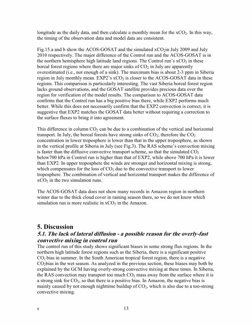
4. Results4.1. Inter-comparison of the three simulationsFig.2 is a comparison of the July monthly mean surface CO2 of the three runs with the different convective transport schemes. The model output every three hours. The monthly means here are full average across day and night. It is found that the surface CO2 of EXP3, which uses the convective transport scheme of the GEOS-Chem CTM, is very similar to that of the control run. The differences between EXP3 and Control are small. However, the EXP2 surface CO2 is quite different from that of the Control. In the northern high latitude land regions, where it is a vast sink for CO2 in July due to uptake of the vast boreal forests, the EXP2 simulates lower CO2 concentration than the Control and EXP3.

Fig.3 shows the monthly mean vertical profiles of CO2 and CO in several different places and in different seasons. Again, we see that the vertical profiles of EXP3 and Control are well coincident each other, while the EXP2 vertical profiles are different. We have checked the instantaneous vertical profiles in many places all over the world and found that the EXP3 and Control are also coincident each other with only very small differences. Therefore, it can be concluded that the convective transport of Scheme-3 is

s 7

equivalent to that of the RAS scheme when it uses the total cloud mass flux and detrainment from RAS. This is not surprising since Scheme-3 contents the basic budget equations which apply for any mass-flux convection schemes. Therefore when the input is the RAS produced cloud mass flux and detrainment, the convective transport of Scheme-3 should be equivalent to that of the control run.

Now we only need to evaluate the results of Control and EXP2. Fig.3 indicates that the tracer vertical gradient of Control run is much weaker than that of EXP2. This can be more clearly seen in the comparison of the CO profiles, since CO fluxes are all positive but CO2 fluxes can be positive or negative. The CO profiles show significant differenceof the vertical gradient of the two simulations. The much weaker vertical gradient of the Control run indicates a much fast convective transport of the tracers by using the RAS scheme than the bulk diffusive scheme (Scheme-2). The slower convective transport of Scheme-2 explains why the simulated surface CO2 in the boreal forest regions is significantly lower than that of the Control as show in Fig.2. The strong sink there during the summer absorbs CO2 from the atmosphere. With a weaker convective mixing, the CO2 concentration near the surface is lower than in the control run.

Fig.4 shows the monthly mean differences of the control and EXP2 runs for the simulated CO2 on the surface and 300 hPa. In northern winter, the major difference on the surface is in the Amazon rain forest region of the South America, where EXP2’s surface CO2concentration is significantly higher than that of the Control. The maximum difference can be more than 10 ppm. A smaller positive difference is also found in Indonesian region. On 300 hPa the differences are small. In July, the major difference is in the northern hemisphere high latitude boreal forest regions. The surface CO2 of EXP2 is significantly lower than that of Control. The maximum difference is in about -7 ppm in Siberia. In North America’s middle to high latitudes, the monthly mean surface CO2 of EXP2 is also lower than that of the Control, but the magnitude of the difference is only 1 to 3 ppm. On the vast ocean regions, the difference is quite small. On 300 hPa the difference is also mainly in Siberia but sign of the difference is reversed from that on the surface. The EXP2’s CO2 is higher than the control run, although the magnitude of the difference is not large. Thus, the surface CO2 differences of the two runs are in those land regions where both the surface fluxes and convection activities are strong. On the oceans and arid land regions, where the CO2 flux is very small in magnitude, the differences are insignificant.

It is desirable to verify which simulation run, the Control or EXP2, is more realistic in those regions where the simulated CO2 is significantly different.

4.2. The evaluationVarious CO2 observation data are used to evaluate the model results, which include the conventional flask and tower observations of the NOAA Earth System Research Laboratory (ESRL), the ground-based observations of the Total Carbon Column Observing Network (TCCON), and the ACOS-GOSAT satellite observing xCO2 data (Atmospheric CO2 Observations from Space retrievals of the Greenhouse gases Observing Satellite).

s 8

4.2.1. Comparison to the NOAA ESRL’s flask dataThe ESRL’s cooperative air sampling network is an international effort to collect sample air regularly at many sites of the world and to analyze the concentration of greenhouse gases in the laboratory. The flask data of surface CO2 data [Conway et al., 2011] provide the collecting time of the samples, which is mostly in daytime especially noon or afternoon local time at each site. Since CO2 concentration has large diurnal variations on land sites, the concentrations of the collected air samples do not represent the daily mean values and can be much lower. Therefore it is not appropriate to directly compare the monthly mean of the flask and model data. In the model runs, we output the results every three hours. We select the results at the similar local time, as in the flask sample event time, and then calculate the monthly mean. Fig.5 shows the difference of the two methods in calculating the monthly mean model data at HUN. The one with the selected local sample time as mentioned above is well consistent with the observed flask data. But the other one (dashed line) with the direct monthly mean model data is far from realistic. In the summertime, it is much higher than that of the flask data. Fig.5 indicates the importance of taking into account of the diurnal variations in CO2 modeling. The use of hourly CASA-GFED3 NEE data in the experiment makes it possible to simulate the diurnal variation and covariance of terrestrial fluxes with PBL diffusion. If using a monthly NEE flux data, we cannot attain the right diurnal variation.

Fig.6.1 and Fig.6.2 are the comparison of monthly CO2levels at a number of flask observation sites in southern and northern hemispheres respectively. In the southern hemispheric sites, the curves of simulated CO2 are very well consistent with that of the observed, and the differences of Control and EXP2 runs are negligible. In the northern hemispheric sites in summer months, the simulated monthly CO2 concentrations are also well consistent with the observations. But in winter months, the simulated values are mostly higher than the observed by a few ppms in many high latitude sites such as HUN, BAL, BRW, and ALT. We will analyze the reason for this overestimation in northern winter below. In general, the comparison with the flask data shows the online simulations are quite successful.

The differences of surface CO2 of the Control run and EXP2 at the ESRL flask observation sites are not large. In northern summer EXP2 simulates slightly lower CO2 at the northern high latitude flask. The differences are only 1-2 ppm. However, it must be pointed out that the ESRL flask observation sites are mostly in remote regions where the surface CO2 fluxes are weak. Observations are lacking in the strong source and sink land regions such as in Amazon or Siberia. Therefore the flask data does not provide information for verifying which simulation run, the Control or EXP2, is more realistic in these strong source regions. Fortunately, we have some tower observations in the strong source regions such as in Tapajos (Amazon region).

4.2.2. Comparison to the tower observationsThe CO2 data of tall tower observations are particularly useful for evaluating the simulation results. The tower observations are high frequency for day and night. So they can be used to verify the diurnal variations of the simulated CO2. Some of the towers are

s 9

as tall as 400 meters. That height covers the 4 lowest levels of the GEOS-5 model. Therefore tower observations can be used to verify the model vertical profiles, as will be shown below. Another reason why the tower observations are particularly useful to this study is the locations of the towers. Unlike most flask observations, which are located in remote sites where CO2 flux is weak or does not exist, the tower observations are mostly in land regions such as North America and Europe, where the terrestrial sources and sinks are not weak. One particularly important tower observation data is located at the Tapajos national forest (2.86S, 54.96W) of the Amazon region. The Amazon’s vast rain forests are the “lungs” of the Earth. Realistic estimation of the CO2 sources and sinks in the Amazon region can be crucial for estimation of the global CO2 budget. In this section, we use the tower observations at Tapajos of the South America and WLEF and WBI of the North America to verify the simulation results. The tower data at AMT, SCT, WKT and others of the North America are also good data. But the differences of the two simulations at these sites are not very significant, so we will not show here.

The Tapajos tower observing data is from the ONRL DAAC [Hutyra et al., 2008].We use the data at the level of 50 meters to compare to the model’s first level above the ground.Fig.7 shows the observed and simulated hourly CO2 mixing ratio at Tapajos in March2003 and March 2005. The amplitude of diurnal variation of the observed CO2 is huge, often exceeding 50 ppm. The surface layer CO2 reaches minimum in afternoon and maximum in late night in local time. A characteristic is that the building up of CO2concentration in nighttime is very large in the observations, indicating the coupling effect of the high emission of CO2 and low vertical transport of convection and turbulence in the rain forest nighttime. The Control run simulates lower CO2 mixing ratio especially at night. The EXP2 simulated surface CO2 is higher than the Control, although the amplitude of diurnal variation is still smaller than the observed.

The monthly mean Tapajos CO2 mixing ratio at 50m height is shown in Fig.8. The monthly means here include the average of day and night data. In the rain season from December to April, the EXP2 simulation is closer to the observed, and the Control simulation is too low, with a difference of about 5 to 10 ppm. This difference is seen in Fig.4, which shows that the EXP2 surface CO2 in February is higher than the Control in Amazon region by the similar amount. According to the Tapajos data, we can roughly conclude that the Control run simulated surface CO2 in Amazon region is too low, while the EXP2 is more realistic. Fig.8 also shows that in the dry season, which is from June to September, the simulated CO2 of both the Control and EXP2 is much lower than the observed. This indicates that the CASA model may overestimate the uptake of the rainforest in the dry season, which should be improved in the future.

The significant difference of the two simulations in Tapajos must be due to the different convective mixing speeds of the RAS and Scheme-2. This can be seen in Fig.9 that shows the evolution of vertical profiles of CO2 for the two runs. The Control run’s vertical profile is almost homogeneous above the cloud base (about 300-500 m), while the EXP2 profile shows a gradient in the vertical. This clearly indicates that the RAS scheme’s convective mixing is much stronger, which sends the emitted CO2 from the cloud base layer to higher levels. As a result, the building up of surface CO2 in nighttime

s 10

is too weak. EXP2’s build up at nighttime is due mostly to its slower convective transport.

Next we analyze the comparison of the simulations to the tower data at LEF (45.94N, 90.27W) and WBI (41.71N, 91.35W). These sites are in the Midwest of the United States, and the towers are about 400 meters of height. Fig.10 shows the hourly-observed CO2 of the towers at the height of the model’s lowest level at these two sites during the summer season. It is found that the diurnal and synoptic variations of the observed CO2are simulated quite well by the two simulations. The simulated diurnal variation amplitude is similar to the observed at these sites. The simulations also capture the day-to-day fluctuations of the observed CO2.

The realistic simulation of the diurnal and synoptic variations at these sites can be mainly due to the use the hourly terrestrial CO2 flux data. Fig.11 shows the evolution of daily mean NEE and observed and simulated surface CO2 at WBI in July 2010. The synoptic variation of the simulated CO2 is consistent with the observed CO2, and the up and down of day-to-day CO2 concentration is correlated with the synoptic variation of the NEE data. Therefore the 3-hourly NEE data of CASA-GFED3 must include realistic synoptic variations so that the simulated CO2 synoptic variation looks realistic. The realistic simulation of the synoptic variation indicates that the MERRA analysis, which is used in calculating the 3-hourly NEE and used in the online replay runs, must be quite realistic.

The difference of EXP2 and Control runs at LEF and WBI can be seen more clearly in the vertical profile map of Fig.12, which shows the July and January monthly mean vertical profiles of CO2 from the surface to 2000 m of height. The tower’s heights are about 400 m, which covers the lowest four levels of the GCM, so the tower data can be used to compare with the simulated profiles at least for these levels. In July, the Midwest of the US is a sink region due the uptake of the forests and crops, and is also in convection season. Fig.12 shows that the EXP2 CO2 is a 2-3 ppm lower than the Control’s in the levels below 1500 m at both LEF and WBI. The profile curves of the two simulations are similar to the tower observed in the near surface 400 m layer, but the EXP2 profiles seem consistently more close to the tower data. It is also noticed at WBI, where it is in a corn field region in the mid-western US, the simulated surface CO2 of both the control and EXP2 runs is higher than the observed. It is possible that the CO2sink there is somewhat underestimated in the CASA-GFED3 terrestrial flux data.

In January, the profiles of the two runs have no difference since there is no convection activity in winter. From Fig.12 we noticed a phenomenon that compared with the tower observations, there is a positive bias in the simulated CO2 near the surface. On the surface layer the bias is about 5-10 ppm. But the bias decreases with height rapidly. Therefore such positive bias, which is also found in many other flask sites as shown in Fig.4, seems only exist in a very shallow layer near the surface. We will discuss this below after comparing to the observed column mean CO2.

s 11

4.2.3. Comparison to the TCCON dataThe TCCON is a network of ground-based Fourier transform spectrometers that record direct solar spectra [Wunch et al., 2011]. The TCCON xCO2 data were obtained from the TCCON Data Archive operated by the California Institute of Technology. The observed data were processed from event data to hourly data. The model simulated column-mean CO2 data were calculated from the 3-hourly output using an air mass weighted averaging method.

Fig.13 and 14 are some comparisons of the observed and simulated xCO2 at Park Falls (45.94N, 90.27W) and Bialystok (53.23N, 23.03E). The two sites are in North America and Eastern Europe respectively. Fig.13 shows the seasonal variations of xCO2 at the two sites in some years. At Park falls, the seasonal variations of the TCCON observed xCO2and the simulated xCO2 are similar to each other, both highest in April to May and lowest in August to September. The xCO2 seasonal variations at Bialystok are also simulated but in summer months the simulated xCO2 is higher than the observed by about 2 ppm. This positive bias may indicate there is an underestimation of CO2 sink in Eastern Europe in summer.

Fig.14 shows the diurnal and synoptic variations of xCO2 at Park Falls. The TCCON data is only for daytime but the simulated xCO2 is continuous. The diurnal variation of the simulated xCO2is small, only about 1-2 ppm, but the day-to-day synoptic variation can be large. From Fig.14, the up and down of synoptic variations of the observed xCO2 are simulated quite well. The xCO2difference of the two simulations is small at the location of Park Falls. The EXP2’s xCO2 is slightly lower than the Control’s. It is interesting to find that the synoptic variation is different from year to year. For example, the synoptic variation is large in year 2005 summer and 2006 summer but is quite small in 2007 summer. The models also capture this supporting our confidence in the synoptic weather simulation and underlying CASA fluxes.

4.2.4. Comparison to the ACOS-GOSAT dataThe ground-based and aircraft-observed CO2 data are very useful. However, they are too sparse in spatial distributions. Due to practical reasons, observations in some important source and sink regions such as the tropical rain forest and the northern boreal forest regions are scarce. Satellite measurements can be a solution for global coverage of CO2observations. In 2009, the Greenhouse gases Observing Satellite (GOSAT) successfully launched, which uses the TANSO-FTS instrument (thermal and near infrared sensor for CO2 observations-Fourier transform spectrometer) [Kuzeet al, 2009; Yokotaet al, 2009]. After the launch, the NASA Atmospheric CO2 Observations from Space (ACOS) team joined the GOSAT team in analyzing GOSAT observations. The goal is to retrieve the column-averaged dry-air mole fraction of CO2, called xCO2. There have been several versions of the ACOS-GOSAT products. The version we used for this study is the ACOS v2-10 [Osterman et al., 2012; O’Dell et al., 2012].

The model-simulated 3-hourly column mean CO2was calculated from the high frequency output of the simulation runs. Since the GOSAT observation is always at about 1:00 pm of the local sun time, we picked up the model data at the similar local time for each

s 12

longitude as the daily data, and then calculate a monthly mean for the xCO2. In this way, the timing of the observation data and model data are consistent.

Fig.15.a and b show the ACOS-GOSAT and the simulated xCO2in July 2009 and July 2010 respectively. The major difference of the Control run and the ACOS-GOSAT is in the northern hemisphere high latitude land regions. The Control run’s xCO2 in these boreal forest regions where there are major sinks of CO2 in July are apparently overestimated (i.e., not enough of a sink). The maximum bias is about 2-3 ppm in Siberia region in July monthly mean. EXP2’s xCO2 is closer to the ACOS-GOSAT data in these regions. This comparison is particularly interesting. The vast Siberia boreal forest region lacks ground observations, and the GOSAT satellite provides precious data over the region for verification of the model results. The comparison to ACOS-GOSAT data confirms that the Control run has a big positive bias there, while EXP2 performs much better. While this does not necessarily confirm that the EXP2 convection is correct, it is suggestive that EXP2 matches the GOSAT data better without requiring a correction to the surface fluxes to bring it into agreement.

This difference in column CO2 can be due to a combination of the vertical and horizontal transport. In July, the boreal forests have strong sinks of CO2; therefore the CO2concentration in lower troposphere is lower than that in the upper troposphere, as shown in the vertical profile at Siberia in July (see Fig.3). The RAS scheme’s convection mixing is faster than the diffusive convective transport scheme, so that the simulated CO2below700 hPa in Control run is higher than that of EXP2, while above 700 hPa it is lower than EXP2. In upper troposphere the winds are stronger and horizontal mixing is strong, which compensates for the loss of CO2 due to the convective transport to lower troposphere. The combination of vertical and horizontal transport makes the difference of xCO2 in the two simulation runs.

The ACOS-GOSAT data does not show many records in Amazon region in northern winter due to the thick cloud cover in raining season there, so we do not know which simulation run is more realistic in xCO2 in the Amazon.

5. Discussion5.1. The lack of lateral diffusion - a possible reason for the overly-fast convective mixing in control runThe control run of this study shows significant biases in some strong flux regions. In the northern high latitude forest regions such as the Siberia, there is a significant positive CO2 bias in summer. In the South American tropical forest region, there is a negative CO2bias in the wet season. As analyzed in the previous section, these biases may both be explained by the GCM having overly-strong convective mixing at these times. In Siberia, the RAS convection may transport too much CO2 mass away from the surface where it is a strong sink for CO2, so that there is a positive bias. In Amazon, the negative bias ismainly caused by not enough nighttime buildup of CO2, which is also due to a too-strong convective mixing.

s 13

The overestimation of convective mixing with the RAS scheme has been known for a long time. Allen et al. [1997] found that the RAS convection scheme tends to move tracers from the planetary boundary layer to the upper troposphere directly, which causes unrealistic “C-like” profiles of 222Rn and an overestimation of CO in tropical upper troposphere in their offline experiments with the GEOS-1 DAS data. They further evaluated the deep convective mixing with the ISCCP (International Satellite Cloud Climatology Project) data, and found the frequency of deep convective mixing appears overestimated and the vertical extent of deep convection in tropics is underestimated in the GEOS-1 DAS, which uses RAS convection scheme. Folkins et al. [2006] also find the too-shallow deep convection with RAS scheme in GEOS-3 DAS. In a recent study about sensitivity of the parameters in RAS scheme on CO simulation, Ott et al. [2011] find that the boundary layer tracers can suddenly appear near the tropopause during a single time step. Our finding that the RAS overestimates the convective mixing is consistent with these former studies.

The comparison of the RAS scheme and the bulk diffusive scheme (Scheme-2) in the CO2 simulations in this study may indicate that lack of lateral mixing between the cumulus plumes and the environmental air in the RAS scheme is an important reason for the overestimation of convective mixing. In the RAS scheme, detrainment is set to happen only at the top of each plume, and there is no lateral diffusion between the plume and the environment air. Therefore there is no any leaking of the tracers from the plume to environment during the convective transport except at the plume top, no matter how tall the plume is. That means that the tracers can directly transport from the cloud base to upper troposphere through the chimney-like tall plumes. This no-leaking assumption could be a reason for the overly efficient convective mixing.

The no-leaking assumption may not be consistent with the cumulus observations in 1980s and 1990s. Raymond and Blyth [1986] and Taylor and Baker [1991] have shown that detrainment can occur anywhere between cloud base and top. Based on such observations, Raymond and Blyth [1986] proposed a “bouncy sorting” model, which was used by the cumulus parameterizations of Kain and Fritsch [1990] and Emanuel [1991]. In the bulk mass-flux cumulus parameterization schemes of Tiedtke [1989] and Gregory and Rowntree [1990], a lateral mixing detrainment term is also incorporated to represent the effect of lateral diffusion at the cloud edge. In recent years, it is increasingly clear that correct representation of the lateral entrainment and detrainment is of key importance in cumulus parameterizations [de Rooy et al., 2011; Bethtold et al., 2008; Derbyshire et al.,2011; etc.].It is not clear yet whether the multi-plume mass flux schemes such as RAS can be improved by introducing the lateral diffusion detrainment.

The simple diffusive convective transport scheme (Scheme-2) that is used in EXP2 assumes the tracer gases in the clouds and the environment are totally mixed. This is the opposite extreme to the no leaking scheme. The EXP2 run shows significant improvement in the simulated CO2, which must be due to the slower convective transport. However, the real situation in cumulus convections must be between the no-leaking and the totally mixing between clouds and environment. Therefore the simple

s 14

diffusive scheme is not the final solution but only a fixer to the convective transport of the current GCM.

5.2. Are the CO2 sources overestimated or there is a missing sink?The comparison of surface CO2 of the multi-year runs with the flask observations (Fig.6)indicates that in the northern hemisphere winter, there exists a positive bias in many land observation locations. The magnitude of the bias varies from place to place, year to year. Sometimes the bias can be as large as 5-10 ppm in monthly means. The simulated surface CO2 in summer is close to the flask observations. Therefore, in taking the annual mean, the inter-hemispheric gradient of the simulated surface CO2 must be larger than the observed because of the overestimation in northern hemisphere winter surface CO2(figure not shown).

However, it turns out that the positive bias only exists in a very shallow layer near the surface, not in the total column. As shown in the monthly mean vertical profiles of the model with the tall towers at LEF and WBI (Fig.12), the positive bias is only in a shallow layer near the surface. In the comparison of the simulated xCO2 with the TCCON observations (Fig.13), there is no such positive bias in the simulated xCO2 in northern winter at Park Falls (North America) and Bialystok (Europe), which indicates that there is no such positive bias in the simulated column total CO2 mass. Therefore the total CO2flux in northern hemisphere is not overestimated. The shallow bias is more likely just due to an underestimation of the turbulence transport near the surface in the GCM.

The above fact indicates that only using the near surface observations to constrain the CO2 sources is insufficient. We can’t make a conclusion based only on the surface observations that the positive bias in inter-hemispheric gradient of the simulated surface CO2 is due to errors in the emissions. The observations of xCO2 can be more useful to verify whether the total fluxes are overestimated or not.

6. SummaryIn this study, multi-year CO2 simulations are conducted with the GEOS-5 GCM and with the land and oceanic surface CO2 flux data of the CASA-GFED3 and NOBM as well as the ORNL’s fossil fuel emission. Three convective transport algorithms are used for the simulation experiments. The results are compared with the various observations including the near surface and the GOSAT satellite observations. The major conclusions are as follows:� CO2 simulations are sensitive to representation of convective transport. Significant differences are found in online simulations that use three different convective transport algorithms. � The multi-plume mass flux convection scheme of the GCM tends to overestimate the convective mixing speed, which leads to large biases in land regions with strong terrestrial fluxes during the convection seasons. � Overall the simulations are quite realistic, especially the one with a simple diffusive convective transport scheme. Due to the advances in the surface flux estimation and in the global observations, CO2 can be a useful tracer for evaluation of the atmospheric models.

s 15

� The lack of lateral diffusion between the cumulus plumes and the environment air can be an important reason for the too fast convective mixing with the AS type’s cumulus parameterizations.

AcknowledgmentsWe would like to acknowledge to the NOAA ESRL for providing the flask and tower observational data of CO2. The Tapajos tower data was from the ONRL DAAC. The ACOS-GOSAT data was from C. O’Dell. Thanks to A. Schuh for the valuable comments. The NASA Carbon Cycle Science funded this research.

References

Allen, D. J., K. E. Pickering, and A. Molod (1997), An evaluation of deep convective mixing in the Goddard chemical transport model using International Satellite Cloud Climatology Project cloud parameters. J. Geophys. Res., 102, 25467-25476.

Andres, R.J., J.S. Gregg, L. Losey, G. Marland, and T.A. Boden (2011), Monthly, global emissions of carbon dioxide from fossil fuel consumption. Tellus, 63B, 309-327.

Arakawa, A., and W. H. Schubert (1974), Interaction of a cumulus cloud ensemble with the large-scale environment. Part I. J. Atmos. Sci., 31, 674-701.

Baker, D.F., et al. (2006),TransCom 3 inversion intercomparison: Impact of transport model errors on the interannual variability of regional CO2 fluxes, 1988-2003, Global Biogeochem. Cycles,20, GB1002, doi:10.1029/2004GB002439.

Bethtold, P., M. Koehler, T. Jung, F. Doblas-Reys, M. Leutbecher, M. Rodwell, F. Vitart, and G. Balsamo (2008), Advances in simulating atmospheric variability with the ECMWF model: From synoptic to decadal time-scales. Q. J. R. Meteorol.. Soc. 134,1337-1351.

Bey, I., et al. (2001), Global modeling of tropospheric chemistry with assimilated meteorology: Model description and evaluation.J. Geophys. Res., 106, 23073-23095.

Bian, H., S.R. Kawa, M. Chin, S. Pawson, Z. Zhu, P. Rasch, and L. Wu (2006), The of representation of convective cloud transport in a model of CO2 transport. Tellus, Vol 58, Issue 5, 463-475.

Bosilovich, M., F. Robertson, and J. Chen (2011), Global energy and water budgets in MERRA. J. Climate, 24, 5721-5739.

Conway, T.J., P.M. Lang, and K.A. Masarie (2011), Atmospheric carbon diozide dry air mole fractions from the NOAA ESRL carbon cycle cooperative global air sampling network, 1968-2010, Version: 2011-10-14, Path: ftp://ftp.cmdl.noaa.gov/ccg/CO2/flask.

s 16

Derbyshire, S.H., A.V. Maidens, S.F. Miltion, E.A. Stratton, and M.R. Willett (2011),Adaptive detrainment in a convective parameterization.Q. J. R. Meteorol.. Soc., 137,1856-1871.

de Rooy, W.C., et al.(2013), Entrainment and detrainment in cumulus convection: an overview. Q. J. R. Meteorol.. Soc. 139, 1-19.

Donner, L. J., L. W. Horowitz, A. M. Fiore, C. J. Semen, D. R. Black, and N. J. Blake(2007), Transport of radon-222 and methyl iodide by deep convection in the GFDL global atmospheric model AM2. J. Geophys. Res., 112, D17303, doi:10.1029/2006JD007548.

Emanuel, K. A. (1991), A scheme for representing cumulus convection in large-scale models. J. Atmos. Sci., 48, 2313-2335.

Gurney, K. R., et al. (2003),TransCom 3 CO2 inversion intercomparison: 1. Annual mean control results and sensitivity to transport and prior flux information. Tellus B, 55, 555-579.

Gregg, W.W., and N.W. Casey (2007), Modeling coccolithophores in the global oceans. Deep Sea ResearchII 54: 447-477.

Gregg, W.W., N.W. Casey, and C.S. Rousseaux (2012), Global surface ocean estimates in a model forced by MERRA. NASA Global Modeling and Assimilation Series, M. Suarez, ed., NASA Technical Memorandum 2012-104606, Vol.31, 32pp.

Gregory, D., and P. R. Rowntree (1990),A mass flux convection scheme with representation of cloud ensemble characteristics and stability dependent closure. Mon. Wea. Rev., 118, 1483-1506.

Hutyra, L.R., J.W. Munger, E.W. Gottlied, B.C. Daube, P.B. Camargo and S.C. Wofsy (2008), LBA-ECO CD-10 CO2 profiles at km 67 tower site, Tapajos National Forest. Data set available on-line [http://www.dacc.ornl.gov] from Oak Ridge National Laboratory distributed active archive center, Oak Ridge, Tennessee, U.S.A. doi:10.3334/ORNLDAAC/855.

Kain, J. S., and J. M. Fritsch (1990), A one-dimensional entraining/detraining plume model and its application in convective parameterization. J. Atmos. Sci., 47, 2784-2802.

Kawa, S. R., D. J. Erickson III, S. Pawson, and Z. Zhu (2004), Global CO2transport simulations using meteorological data from the NASA data assimilation system. J. Geophys. Res., 109, D18312,doi:10.1029/2004JD004554.

s 17

Kuze, A., H. Suto, M. Nakajima, and T, Hamazaki (2009), Thermal and near infrared sensor for carbon observation Fourier-transform spectrometer on the Greenhouse Gases Observing Satellite for greenhouse gases monitoring, Appl. Opt., 48, 6716-6733.

Law, R.M. et al. (2008), TransCom model simulations of hourly atmospheric CO2:Experimental overview and diurnal cycle results for 2002. Global Biogeochemical cycles,22, GB3009, doi:10.1029/2007GB003050.

Lin, S. J. (1996), Description of the parameterization of cumulus transport in the 3D Goddard chemistry transport model. Office Note, NASA/GSFC, 5pp.

Lin, S. J. (2004), A vertically Lagrangian finite-volume dynamical core for global models.Mon. Wea. Rev., 132, 2293-2307.

Los, S.O., N.H. Pollack, M.T. Parris, G.J. Collatz, C.J. Tucker, P.J. Sellers, C.M. Malmstrom, R.S. DeFries, L. Bounoua, and D.A. Dazlich (2000), A global 9-yr biophysical land surface dataset from NOAA AVHRR data. J. Hydrometeorology,1, 183-199.

Mahowald, N. M., P. Rasch, and R. G. Prinn (1995), Cumulus parameterizations in chemical transport models. J. Geophys. Res., 100, 26173-26189.

Moorthi, S. and M. J. Suarez (1992) Relaxed Arakawa-Schubert: A parameterization of moist convection for general circulation models. Mon. Wea. Rev., 120, 978-1002.

O’Dell, C.W. et al. (2012), The ACOS CO2 retrieval algorithm – Part 1: Description and validation against synthetic observations. Atmos. Meas. Tech., 5, 99-121, 2012.

Olsen, S.C., and J.T. Randerson (2004), Differences between surface and column atmospheric CO2 and implications for carbon cycle research.J. Geophys. Res., 109,D02301, doi:10.1029/2003JD003968.

Osterman, G., A. Eldering, C. Avis, C. O’Dell, E. Martizez, and D. Crisp(2012), ACOS Level 2 Standard Product Data User’s Guide, v2.10. Goddard Earth Science Data Information and Services Center (GES DISC).

Ott, L., S. Pawson, and J. Bacmeister (2011), An analysis of the impact of convective parameter sensitivity of simulated global atmospheric CO distributions, J. Geophys. Res.,116, D21310, doi:10.1029/2011JD016077.

Pan, H.-L., and W.S. Wu (1995),Implementing a mass flux convective parameterization package for the NMC Medium-Range Forecast model. NMC Office Note 409, 40pp.

Potter, C. S., Randerson, J. T., Field, C. B., Matson, P. A., Vitousek, P. M., Mooney, H. A., and Klooster, S. A.(1993), Terrestrial ecosystem production – A process model based on global satellite and surface data, Global Biogeochem. Cycles, 7, 811–841.

s 18

Randerson J.T., M.V.Thompson, C.M. Malmstrom (1996),Substrate limitations for heterotrophs: Implications for models that estimate the seasonal cycle of atmospheric CO2. Global Biogeochemical Cycles 10, 585-602.

Raymond, D.J., and A.M. Blyth (1986), A stochastic mixing model for non-precipitating cumulus clouds.J. Atmos. Sci. 43, 2708-2718.

Rienecker M.M., et al. (2008), The GEOS-5 Data Assimilation System – Documentation of version 5.0.1 and 5.1.0 and 5.2.0. NASA Tech. Rep. Series on Global Modeling and Data Assimilation, NASA/TM-2008-104606, 27, 92pp.

Stommel, H. (1947), Entrainment of air into a cumulus cloud. J. Meteor., 4, 92-94

Taylor, G. R., and M. B. Baker (1991), Entrainment and detrainment in cumulus clouds.J. Atmos. Sci., 48, 112-121.

Tiedtke, M. (1989), A comprehensive mass flux scheme for cumulus parameterization in large-scale models. Mon. Wea. Rev., 117, 1779-1800.

Tucker, C.J., J.E. Pinzon, M.E. Brown, D.A. Slayback, E.W. Pak, R. Mahoney, E.F. Vermote, and N. El Saleous (2005), An extended AVHRR 8-km NDVI dataset compatible with MODIS and SPOT vegetation NDVI data. International Journal of Remote Sensing, 26, 4485-4498.

Warner, J.(1970),On steady-state one-dimensional models of cumulus convection. J. Atmos. Sci., 27, 1035-1040.

Warner, J., M. McCourt, C. D. Barnet, W. W. McMillan, W. Wolf, E. Maddy, and G. Sachse(2007), A comparison of satellite tropospheric carbon monoxide measurements from AIRS and MOPITT during INTEX-A. J. Geophys. Res., 112, D12S17, doi:10.1029/2006JD007925.

van der Werf G.R., J.T. Randerson, L. Giglio, G.J. Collatz, P.S. Kasibhatla, A.F. Arellano Jr(2006),Interannual variability of global biomass burning emissions from 1997 to 2004. Atmospheric Chemistry and Physics6, 3423-3441

van der Werf, G.R., J.T. Randerson, L. Giglio L, G.J. Collatz, M. Mu, P.S. Kasibhatla,D.C. Morton, R.S. DeFries, Y. Jin, T.T. van Leeuwen(2010), Global fire emissions and the contribution of deforestation, agriculture, and peat fires (1997-2009). Atmospheric Chemistry and Physics10, 11707-11735

Wunch, D., G.C. Toon, J. Blavier, R.A. Washenfelder, J. Notholt, B.J. Connor, D.W.T. Griffith, V. Sherlock, P.O. Wennberg (2011), The Total Carbon Column Observing Network. Phil. Trans. R. Soc. A, 369, doi:10.1098/rsta.2010.0240.

s 19

Yokota, T. et al. (2009), Global concentrations of CO2 and CH4 retrieved from GOSAT. SOLA, 5, 160-163.

Zhang, K., H. Wan, M. Zhang, and B. Wang (2008), Evaluation of the atmospheric transport in a GCM using radon measurements: sensitivity to cumulus convection parameterization. Atmos. Chem. Phys., 8, 2811-2832.

Figure1. Time series of monthly (upper panel) and yearly (lower panel) global total CO2fluxes for the terrestrial biota, biomass burning, oceanic fCO2, fossil fuel combustion and the sum. The unit is Pg C/year.

s 20

Figure 2. Simulated monthly mean surface CO2 concentration in July 2003 for the Control run and EXP2, EXP3 runs, respectively.

s 21

Figure 3.Monthly mean vertical profiles of CO2 and CO at some land places.

s 22

Figure 4. Difference of monthly mean CO2 at surface and 300 hPa (EXP2 – Control) in February and July 2009. Unit is ppmv.

s 23

Figure 5.Comparison of monthly mean surface CO2at HUN using two methods. Oneis calculated from the daily means (dashed green line). The other is calculated from the daily values at local time afternoon (solid green line). The red line is from the flask observations.

s 24

Figure 6. Time series of monthly mean surface CO2 for 2003-2010 at a number of flask sites. The upper six and lower six are in the southern and northern hemispheres respectively.

s 25

Fig. 7. Time series of the simulated and the tower observed hourly surface CO2at Tapajos in raining season. The observed CO2 is from the tower data at 50 m level that is consistent to the lowest model level.

s 26

Figure 8. Time series of monthly mean CO2 of the simulated and observed at Tapajos.

s 27

Figure 9. Time evolution of vertical profiles of CO2 at Tapajos for Control (upper panel) and EXP2 (lower panel) runs respectively.

s 28

Figure 10. Time series of hourly surface CO2 at LEF and WBI. The simulated CO2 is at the lowest model level (52 m), and the observed data is interpolated to the similar height.

s 29

Figure 11. Daily mean CO2 (upper panel) and daily mean NEE (lower panel) at WBI.

s 30

Figure 12. Monthly mean vertical profiles of CO2 at LEF and WBI. Upper: in July, lower: in January.

s 31

Figure 13. Time series of the TCCON xCO2 and simulated xCO2 at Park Falls (45.94N, 90.27W) and Bialystok (52.23N, 23.03E).

s 32

Figure 14. July time series of the simulated and the TCCON observed xCO2 at Park Falls.

s 33

Figure 15a. Comparison of the ACOS-GOSAT observed xCO2 with the simulated xCO2of the Control and EXP2 runs in July 2009.

s 34

Figure 15b. Same as the Fig.15a but for July 2010.

s 35