IEEE GEOSCIENCE AND REMOTE SENSING LETTERS, VOL. 7, NO. 4, OCTOBER 2010 751

Sensitivity of AMSR-E Brightness Temperatures tothe Seasonal Evolution of Lake Ice Thickness

Kyung-Kuk Kang, Student Member, IEEE, Claude R. Duguay, Stephen E. L. Howell,Chris P. Derksen, and Richard E. J. Kelly, Member, IEEE

Abstract—The sensitivity of brightness temperature (TB) at6.9, 10.7, and 18.7 GHz from Advanced Microwave ScanningRadiometer—Earth Observing System (AMSR-E) observations isinvestigated over five winter seasons (2002–2007) on Great BearLake and Great Slave Lake, Northwest Territories, Canada. TheTB measurements are compared to ice thicknesses obtained witha previously validated thermodynamic lake ice model. Lake icethickness is found to explain much of the increase of TB at 10.7 and18.7 GHz. TB acquired at 18.7 GHz (V-pol) and 10.7 GHz (H-pol)shows the strongest relation with simulated lake ice thickness overthe period of study (R2 > 0.90). A comparison of the seasonalevolution of TB for a cold winter (2003–2004) and a warm winter(2005–2006) reveals that the relationship between TB and icegrowth is stronger in the cold winter (2003–2004). Overall, thisletter shows the high sensitivity of TB to ice growth and, thus,the potential of AMSR-E mid-frequency channels to estimate icethickness on large northern lakes.

Index Terms—Advanced Microwave Scanning Radiometer—Earth Observing System (EOS) (AMSR-E), brightness tempera-ture, ice thickness, lakes, radiometry.

I. INTRODUCTION

LAKE ice grows steadily between the end of the freeze-upperiod and the onset of the break-up period as a result of

the thermodynamics of freezing water and dynamic ice motionon the surface. Lake ice thickens as a result of two fundamentalformation processes: 1) Black ice (congelation ice) is created bythe heat transfer of freezing water at the ice–water interface, and2) snow ice is created by the freezing of slush at the snow–iceinterface. Negative temperature gradients in the ice and snow(for black ice) and snow alone (for snow ice) cause conductiveheat flow through the insulating ice layer into the subzeroatmosphere [1]. In thermodynamic thickening, this conductiveheat flow controls the ice growth rate and the ice thickness [1],and the ice thickens downward as a result of heat loss at the topof the ice/snow cover.

Manuscript received November 25, 2009; revised February 11, 2010. Date ofpublication May 17, 2010; date of current version October 13, 2010. The workof C. Duguay was supported by a Natural Sciences and Engineering ResearchCouncil of Canada Discovery grant.

K.-K. Kang, C. R. Duguay, and R. E. J. Kelly are with the InterdisciplinaryCentre on Climate Change (IC3) and the Department of Geography andEnvironmental Management, University of Waterloo, Waterloo, ON N2L 3G1,Canada (e-mail: kkkang@uwaterloo.ca; crduguay@connect.uwaterloo.ca;rejkelly@connect.uwaterloo.ca).

S. E. L. Howell and C. P. Derksen are with the Climate Research Division,Science and Technology Branch, Environment Canada, Toronto, ON M3H 5T4,Canada and also with IC3 and the Department of Geography and EnvironmentalManagement, University of Waterloo, Waterloo, ON N2L 3G1, Canada (e-mail:Stephen.Howell@ec.gc.ca; chris.derksen@ec.gc.ca).

Color versions of one or more of the figures in this paper are available onlineat http://ieeexplore.ieee.org.

Digital Object Identifier 10.1109/LGRS.2010.2044742

The timing of ice formation and decay, ice cover dura-tion, and ice growth play an important role in the surfaceenergy/water budget and greenhouse gas budgets at regionalscales where lakes occupy a significant fraction of the land-scape. In particular, the total conductive heat loss resulting fromwintertime ice growth has been shown to play a significant rolein the energy balance of the lake-rich area of the North Slopeof Alaska, and areas occupied by large deep lakes [e.g., GreatSlave Lake (GSL)] relative to other lakes in their immediate sur-roundings [1]. In addition to their role in regional climate, mid-to high-latitude lakes are also sensitive indicators of changingclimate conditions. Recent studies using ice phenological ob-servations from a historical Canadian database have shown thesensitivity of lake ice cover during the second half of the twen-tieth century to climate warming and to large-scale atmosphericteleconnection patterns [2]. Unfortunately, Canada’s historicalground-based observational network, which has provided muchof the evidence for the documented changes and links to atmo-spheric forcings and which included weekly/biweekly ice thick-ness measurements, has almost totally disappeared over the lasttwo decades [3]. Satellite remote sensing, particularly those sen-sors operating at microwave frequencies, provides a potentialmeans for obtaining frequent ice thickness estimates from space.

A few studies have shown the potential of spaceborne passivemicrowave radiometry, alone or in combination with radaraltimetry, for the retrieval of information regarding lake icephenology (i.e., timing of ice-on and ice-off dates, and icecover duration) [4], [5]. There has also been some demonstra-tion of the utility of brightness temperature (TB) from pas-sive microwave airborne radiometers to estimate ice thickness[6]–[8]. In particular, a previous study by Hall et al. in 1981showed, although with only four days of airborne/field mea-surements during an entire winter period, a strong positiverelationship between TB at low frequency (5–6 GHz) andlake ice thickness. The availability of frequent (twice-daily)TB measurements from the Advanced Microwave ScanningRadiometer—Earth Observation System (EOS) (AMSR-E)satellite sensor provides an opportunity to examine more thor-oughly the strength of this relationship.

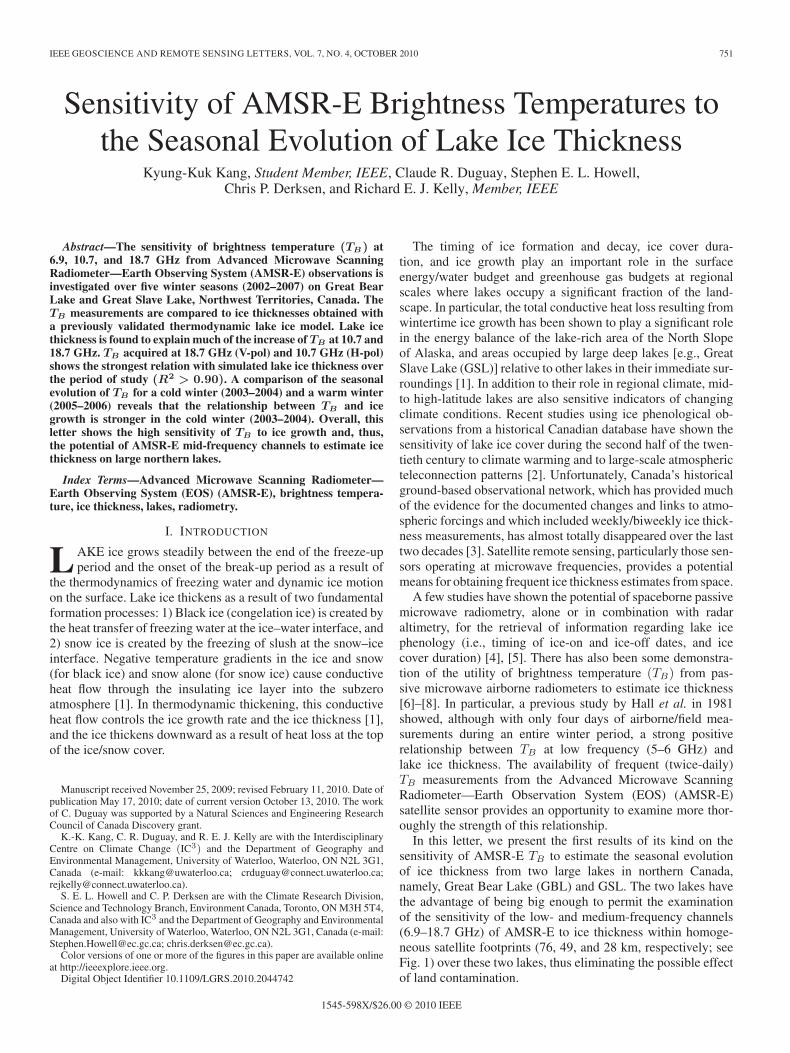
In this letter, we present the first results of its kind on thesensitivity of AMSR-E TB to estimate the seasonal evolutionof ice thickness from two large lakes in northern Canada,namely, Great Bear Lake (GBL) and GSL. The two lakes havethe advantage of being big enough to permit the examinationof the sensitivity of the low- and medium-frequency channels(6.9–18.7 GHz) of AMSR-E to ice thickness within homoge-neous satellite footprints (76, 49, and 28 km, respectively; seeFig. 1) over these two lakes, thus eliminating the possible effectof land contamination.

1545-598X/$26.00 © 2010 IEEE

752 IEEE GEOSCIENCE AND REMOTE SENSING LETTERS, VOL. 7, NO. 4, OCTOBER 2010

Fig. 1. Map showing the locations of GBL, GSL, and nearby meteorologicalstations (Deline, Yellowknife, and Hay River) within MRB. The solid blacksquares represent 5.1′ × 5.1′ of the sampling area on both GBL and GSL. Theblack, dark-gray, and bright-gray open circles indicate the diameters of differentfootprints at (black, 76 km) 6.9 GHz, (dark gray, 49 km) 10.65 GHz, and (brightgray, 28 km) 18.7 GHz, respectively.

TABLE IMEAN TEMPERATURE (IN DEGREES CELSIUS) IN JANUARY (JULY)AND TOTAL ANNUAL SNOWFALL (IN CENTIMETERS) RECORDED

AT DELINE (GREAT BEAR LAKE), YELLOWKNIFE, AND HAY RIVER

(GREAT SLAVE LAKE) METEOROLOGICAL STATIONS

II. DATA AND METHODS

GBL and GSL are located in the Mackenzie River Basin(MRB; Fig. 1) and rank among the ten largest freshwater lakesin the world. GBL and GSL lie between 60◦ and 67◦ N and109◦ to 126◦ W (Fig. 1), with surface areas (average depths) of31 153 km2 (76 m) and 28 450 km2 (88 m), respectively [9]. Asummary of January and July temperature and snow precipita-tion measured at coastal weather stations is provided in Table Ifor the 2002 to 2007 period of analysis described in this letter.The mean air temperature in the GSL area is generally warmerthan that of GBL, and therefore, GSL has an open-water seasonabout four to six weeks longer than GBL [10]. The lake is ice-free from the beginning of June until mid- to late-December,and lake ice conditions on this lake have been reported toexhibit greater inter-annual variability than on GBL [11].

The evolution of TB (horizontal and vertical polarizations;55◦ incidence angle) derived from the AMSR-E/Aqua level-2A global swath spatially resampled brightness temperatureproduct (AE_L2A) was compared to ice thickness obtainedwith the Canadian Lake Ice Model (CLIMo) [12] for the period2002–2007 at both GBL and GSL, since insufficient ground-based measurements are available for a suitable comparison.The 1-D thermodynamic lake ice model has been shown toprovide good estimates of ice thickness on a daily basis, aswell as the freeze-up and break-up dates on shallow lakesnear Fairbanks (Alaska), and Churchill (Manitoba) [12], andon large lakes such as GSL [13]. TB data were acquiredfrom the AMSR-E sensor for both descending and ascendingoverpasses. To examine the sensitivity of TB at 6.9, 10.7,and 18.7 GHz (horizontal and vertical polarizations) to icethickness, all AMSR-E observations for each day falling withina 5.1′ × 5.1′ grid overlapping area between descending andascending modes in AMSR-E were averaged over the areas ofinterest, within the central sections of GBL (66◦ N, 120◦30′ W)and GSL (61◦19.8′ N, 115◦ W and 61◦41.8′ N, 113◦49.5′ W)(Fig. 1). During the data collection, any TB that was recordedwhen the maximum daily air temperatures were above 0 ◦C formore than four consecutive days at the nearby meteorologicalstations was excluded to eliminate days possibly affected bysurface melt, which affects TB values. During surface meltevents, TB values are not representative of the seasonal evo-lution of ice thickness.

To examine the relation between TB and ice thickness,daily ice thicknesses were simulated from CLIMo on bothlakes by performing a simulation over the period 2002–2007.The model was forced with mean daily air temperature,wind speed, relative humidity, cloud cover, and snowfall mea-surements available from the Deline (65◦12′ N, 123◦26′ W)meteorological station for GBL, and using the station datafrom Yellowknife (62◦27.6′ N, 114◦26.4′ W) and Hay River(60◦50.4′ N, 115◦46.8′ W) for GSL (see Fig. 1). For simulatingice thickness on GBL and GSL with CLIMo, a 40-m meanmixing depth and a 25% snow scenario were selected becauseprevious research indicates that GSL has a 40-m mixing layerdepth at the onset of ice formation [10], which is also likelysimilar over GBL. The scenario of 25% snow cover over lakeice, which corresponds to 25% of the snow depth measuredat the closest meteorological station, was applied to provide amore realistic representation of snow accumulation on the icesurface of the lakes, as snow is strongly redistributed by windson these lakes during the course of a typical winter season [12].This scenario has been shown to provide good estimates of icethickness with CLIMo in a previous investigation on GSL [13].

Simple linear regression was applied to determine the fre-quencies and polarizations (significance at p < 0.05) that weremost sensitive to ice thickness over the five winter seasons(2002–2007). The coefficient of determination (R2) was alsocalculated to quantify the variability of TB explained by sea-sonal ice thickening.

III. RESULTS AND DISCUSSION

A. General Evolution of TB From Initial Ice Formation to Melt

Lake ice formation, growth, and decay on GBL and GSLencompass fall freeze-up; a long winter period of ice growth

KANG et al.: SENSITIVITY OF AMSR-E BRIGHTNESS TEMPERATURES 753

Fig. 2. Time series of (top) horizontal-polarization and (middle) vertical-polarization brightness temperatures at 6.9, 10.7, and 18.7 GHz on GBL fromthe 2003–2004 winter period. The time series of (Max_T, red) maximum and(Mean_T, blue) mean air temperatures obtained at Deline is shown at the bottomof the figure with (gray) snow depth. Simulated ice thicknesses in the winterof 2003-2004 obtained with CLIMo (details given in the text) are representedby the thick gray curve. The two red circles overlaid on the ice thicknesscurve correspond to in situ measurements made during field visits on GBL(65◦15′ N, 122◦51.5′ W).

and thickening; a short period of ice melting and thinning; and,eventually, spring break-up and the complete disappearance ofthe ice cover. Ice growth (thickening) is influenced mainly byair temperature and the presence of snow on the ice surface.At the frequencies examined in this letter, the effect of theatmosphere can largely be ignored such that variations in TB aredetermined by emissivity and physical temperature changes ofthe medium. In addition to the properties of the medium underinvestigation, emissivity and, thus, TB also vary with frequencyand polarization (with the incidence angle being fixed at 55◦ forAMSR-E).

As shown in Fig. 2, using the footprint centered on GBLas an example, when air temperature drops below 0 ◦C, theexpected change of TB in response to lake ice formation isdelayed due to the heat capacity in large lakes. Four to sixweeks after air temperature started to decrease below 0 ◦C,the TB over the lake starts to increase due to the increase inice fraction. From the first appearance of ice, it takes threeto five weeks for complete freeze over (CFO) to occur (i.e.,full sheet of ice to form within the footprint of interest).This process is more strongly apparent at H-polarization (topgraphic of Fig. 2), where TB increases by about 70 K fromopen water to CFO conditions. Ice then starts to thicken (mid-December on GBL and late December on GSL; not shown) and

reaches its maximum thickness (thick gray curve in the bottomgraphic of Fig. 2) just before the beginning of melt onset (MO),when the mean air temperature starts to exceed 0 ◦C. Whenthis temperature is reached, TB increases rapidly due to thehigher air temperature and increasing shortwave flux absorptionon the lake ice/snow surface from melt. During this period,melt/refreeze (day/night) events cause fluctuations in TB alongthe general spring-melt trajectory (from MO onward). A similarprocess occurs over GSL (not shown).

B. Relation Between TB and Lake Ice Thickness

For freshwater ice with few scatterers (e.g., trapped air bub-bles created during freezing), the emissivity is predominatelyaffected by the ice/air interface, the ice/water interface, and theice thickness. Early studies have shown that a uniform bubble-free slab of lake ice emits microwave radiation in a quantity thatis proportional to its thickness [6]–[8]. The penetration depthin freshwater ice is well known to decrease with increasingfrequency. Also, the temperature dependence of the imaginarypart of the dielectric constant causes the penetration depthto decrease with increasing temperature. For example, for icewithout impurities, penetration depths at 6.6/10.7/18/37 GHzhave been reported to be on the order of 19/8/2.8/0.7 m at−8.15 ◦C and 34/12/4.5/0.9 m at −43.15 ◦C [14]. Given this,the low- to mid-frequency channels available on the AMSR-Eplatform (6.9, 10.7, 18.7 GHz) possess penetration depths thatare sufficient to interact with ice and water media and to showthe influence of increasing ice thickness on TB .

Over the winter ice growth period, between CFO and MO,as shown in Fig. 2, TB increases, as expected, since thicker icereduces the influence of the lower emissivity (radiometricallycold) liquid water below the ice and emits its own microwaveenergy [15]. In a previous study [16], the near-nadir mid-winter emissivity of lake ice was estimated to be around 0.9 at18.0 GHz near Pudäsjarvi, Finland, which is much higher thanthat of open water (0.4–0.5). As shown in Fig. 2, between CFOand MO, TB is about 20–30 K higher at vertical polarizationcompared to that at horizontal polarization at all frequencies.TB values are smaller by about 20–30 K at lower frequen-cies (6.9–10.7 GHz) in contrast to that at higher 18.7-GHzfrequency over the full extent of the ice growth season. Since18.7 GHz has a shorter penetration depth than 10.7 and6.9 GHz, it is affected by the underlying radiometrically coldwater only in the early period of winter.

The temperature-vulnerable absorption length of ice causesa wavy pattern in the time series of TB for both lakes, asshown in Figs. 2 and 4. These oscillating characteristics of TB

depend greatly on the imaginary part of the index of refractionof ice. This is more noticeable during the warmer winterseason (2005–2006), which experienced greater air temperaturevariability during the course of the ice growth season.

1) Strength of Relation Over the Full Study Period (2002–2007): The statistics summarized in Table II (average 2002–2007) and the box plots shown in Fig. 3 clearly reveal thestrong relation between simulated ice thickness and TB forall three frequencies examined herein. When all three sitesand years are grouped together, the strongest relation is foundat 10.7- and 18.7-GHz frequencies, with over 90% of thevariations in TB being explained by variations in ice thickness.

754 IEEE GEOSCIENCE AND REMOTE SENSING LETTERS, VOL. 7, NO. 4, OCTOBER 2010

TABLE IICOEFFICIENT OF DETERMINATION (R2) AND REGRESSION SLOPE OF RELATION BETWEEN TB AND ICE THICKNESS FOR COLD WINTER (2003–2004),

WARM WINTER (2005–2006), AND AVERAGE CONDITIONS (2002–2007) FOR SAMPLING FOOTPRINTS AT GBL_D (DELINE), GSL_Y(YELLOWKNIFE), AND GSL_H (HAY RIVER). REGRESSION SLOPES (IN KELVINS PER CENTIMETER) ARE IN BRACKETS

Fig. 3. Boxplots of R2 values between simulated ice thickness (with 40-mmixing depth and 25% snow cover scenario) and brightness temperature at6.9, 10.7, and 18.7 GHz from the sampled AMSR-E footprints shown in Fig. 1(averaged over five winter seasons, 2002–2007), showing the (center lines) me-dian, the (boxes) first- and third-quartile ranges, and the (whiskers) maximumand minimum limits.

The R2 values are slightly higher at vertical polarization forthe 18.7-GHz frequency and at horizontal polarization for the10.7-GHz frequency. Contrary to the results obtained byHall et al. in 1981 with airborne measurements, the relation be-tween TB and ice thickness is weaker, although still significant(p < 0.05), at a lower frequency (6.9 GHz).

Two factors may explain this discrepancy. First, the footprintat 6.9 GHz (75 km × 43 km) is larger than that at 10.7 GHzand even more than that at 18.7 GHz (27 km × 16 km), henceencompassing a larger area on GBL and GSL. The lake icemodel provides a single value of ice thickness over the largefootprint on any day, while the TB values from AMSR-E areinfluenced by the spatial variability in ice thickness, which isknown to vary across lakes. Therefore, the larger footprint at6.9 GHz may include a greater range of ice thicknesses than thatgiven by the ice model. A second factor that may also explainthe lower R2 values at 6.9 GHz is that the footprints of thethree sites may somewhat be influenced by land contamination,although every effort was made to exclude such an effect.Nonetheless, the strong relations found at 10.7 and 18.7 GHzare very promising for future investigations on the estimationof lake ice thickness from AMSR-E.

Fig. 4. Linear regression plots between simulated lake ice thickness andbrightness temperature at 6.9, 10.7, and 18.7 GHz for GBL_D (Deline), GSL_Y(Yellowknife), and GSL_H (Hay River) for a cold winter (2003–2004) and awarm winter (2005–2006). The values (n) in parentheses indicate the numberof paired ice thickness and TB observations.

2) Cold Winter (2003–2004) Versus Warm Winter (2005–2006): Although a strong relation was found to exist betweenTB and ice thickness when the data from all sites and years aregrouped together, it is also worth examining how this relationdiffers, if at all, when comparing a cold winter with a warmwinter. Table II and Fig. 4 reveal that the interannual variabilityof climate affects ice growth and, thus, both the strength of therelation between TB and ice thickness and, to a lesser extent,the slope of the relation between the two variables. Threespecific observations can be drawn from Table II regarding theR2 values. First, the strength of the relation is weaker (i.e.,smaller R2 values) for the warmer winter compared to thecolder winter. This is particularly evident with the January 2004and January 2006 temperatures at the GSL sites (Table I), where

KANG et al.: SENSITIVITY OF AMSR-E BRIGHTNESS TEMPERATURES 755

the TB values exhibit greater interseasonal variability in winter2005–2006 compared to that in 2003–2004 (Fig. 4) due to thelarger fluctuations in air temperature during ice growth. Second,the strength of the relation is always stronger at V-polarizationfor the 18-GHz channel, regardless of the site, while at 10.7and 6.9 GHz, the strongest R2 values are obtained at eitherV- or H-polarization, depending on the site and season (coldversus warm winter). This effect is the subject of ongoinginvestigation. Third, the regression slopes shown in Table IIprovide useful information regarding the rate of change of TB

with ice thickness (in kelvins per centimeter). Steeper slopesare found at H-polarization for all three frequencies. Also,as frequency increases from 6.9 to 18.7 GHz, slopes becomesteeper. For example, the slope at GBL_D (2003–2004) is0.26 K · cm−1 at 18.7 (V) GHz and 0.10 K · cm−1 at 6.9 (V)GHz. Given the strong proportion of variations in TB explainedby ice thickness growth, this relation could potentially beinverted to determine winter ice growth rates (in kelvins percentimeter) and thus estimate ice thickness on these large lakes.

IV. CONCLUSION

This letter has revealed the strong sensitivity of TB fromthe low- and middle-frequency channels (6.9–18.7 GHz) ofAMSR-E to the seasonal evolution of ice thickness on twolarge northern lakes. Using the data from five winter seasons(2002–2007), it has been found that the TB values at 10.7-and 18.7-GHz frequencies were highly correlated with icethickness; the R2 values were on the order of 0.9 when thedata from both lakes and for all years were pooled together.Some differences in the strength of the relation were observedwhen comparing TB and ice thickness estimates from a coldversus a warm winter. The strength of the relation between TB

at 10.7- and 18.7-GHz frequencies and ice thickness was higherfor the colder winter, when less interseasonal variability in airtemperature was observed at meteorological stations located inthe vicinity of the lake sites.

The results presented in this letter are consistent with theresults from an earlier work based on airborne passive mi-crowave measurements coincident with limited ice thicknessobservations (four to six measurement campaigns during a fullwinter from the Walden Reservoir, north-central Colorado),which also found a strong relation between TB and ice thick-ness at frequencies between about 5 and 22 GHz [6]–[8].However, these previous studies showed a higher sensitivity ofTB at 5 GHz (R2 = 0.98) to ice thickness compared to thatat 18.7-GHz frequency (R2 = 0.67). In contrast, using dailyAMSR-E TB measurements at similar frequencies, this lettershows a stronger relation with ice thickness at 18 GHz (R2 =0.86−0.91) and 10 GHz (R2 =0.87−0.90) than that at 6 GHz(R2 = 0.74−0.78). These results indicate that TB measure-ments obtained from AMSR-E offer a high potential for es-timating ice thickness on large northern lakes on a regularbasis.

ACKNOWLEDGMENT

The authors would like to thank P. Ménard for his help withthe numerical lake ice model simulations. The AMSR-E/Aqualevel-2A product (AE_L2A) was obtained from the NationalSnow and Ice Data Center Distributed Active Archive Center,University of Colorado at Boulder.

REFERENCES

[1] M. O. Jeffries and K. Morris, “Instantaneous daytime conductive heat flowthrough snow on lake ice in Alaska,” Hydrol. Process., vol. 20, no. 4,pp. 803–815, Mar. 2006.

[2] B. R. Bonsal, T. D. Prowse, C. R. Duguay, and M. P. Lacroix, “Impacts oflarge-scale teleconnections on freshwater-ice break/freeze-up dates overCanada,” J. Hydrol., vol. 330, no. 1/2, pp. 340–353, Oct. 2006.

[3] F. Lenormand, C. R. Duguay, and R. Gauthier, “Development of a his-torical ice database for the study of climate change in Canada,” Hydrol.Process., vol. 16, no. 18, pp. 3707–3722, Dec. 2002.

[4] A. V. Kouraev, S. V. Semovski, M. N. Shimaraev, N. M. Mognard,B. Legresy, and F. Remy, “Observations of Lake Baikal ice from satel-lite altimetry and radiometry,” Remote Sens. Environ., vol. 108, no. 3,pp. 240–253, 2007.

[5] A. V. Kouraev, S. V. Semovski, M. N. Shimaraev, N. M. Mognard,B. Legrésy, and F. Rémy, “The ice regime of Lake Baikal from historicaland satellite data: Relationship to air temperature, dynamical, and otherfactors,” Limnol. Oceanogr., vol. 52, no. 3, pp. 1268–1286, 2007.

[6] D. K. Hall, J. L. Foster, A. T. C. Chang, and A. Rango, “Freshwater icethickness observations using passive microwave sensors,” IEEE Trans.Geosci. Remote Sens., vol. GRS-19, no. 4, pp. 189–193, Oct. 1981.

[7] D. K. Hall, “Active and passive microwave remote sensing of frozen lakesfor regional climate studies,” in Proc. Snow Watch—Detection StrategiesSnow Ice, Glaciological Data Rep GD-25, 1993, pp. 80–85.

[8] A. T. C. Chang, J. L. Foster, D. K. Hall, B. E. Goodison, A. E. Walker,J. R. Metcalfe, and A. Harby, “Snow parameters derived from microwavemeasurements during the BOREAS winter field campaign,” J. Geophys.Res., vol. 102, no. D4, pp. 29 663–29 671, 1997.

[9] W. R. Rouse, P. D. Blanken, C. R. Duguay, C. J. Oswald,and W. M. Schertzer, “Climate-lake interactions,” in Cold RegionAtmospheric and Hydrologic Studies: The Mackenzie GEWEX Experi-ence, M. K. Woo, Ed. Berlin, Germany: Springer-Verlag, 2008, ch. 8,pp. 139–160.

[10] W. M. Schertzer, W. R. Rouse, P. D. Blanken, A. E. Walker, D. C. L. Lam,and L. Leon, “Interannual variability of the thermal components and bulkheat exchange of Great Slave Lake,” in Cold Region Atmospheric andHydrologic Studies: The Mackenzie GEWEX Experience, M. K. Woo, Ed.Berlin, Germany: Springer-Verlag, 2008, ch. 11, pp. 197–219.

[11] P. Blanken, W. Rouse, and W. M. Schertzer, “Time scales of evaporationfrom Great Slave Lake,” in Cold Region Atmospheric and HydrologicStudies: The Mackenzie GEWEX Experience, M. K. Woo, Ed. Berlin,Germany: Springer-Verlag, 2008, ch. 10, pp. 181–196.

[12] C. R. Duguay, G. M. Flato, M. O. Jeffries, P. Ménard, K. Morris, andW. R. Rouse, “Ice-cover variability on shallow lakes at high latitudes:Model simulations and observations,” Hydrol. Process., vol. 17, no. 17,pp. 3465–3483, Dec. 2003.

[13] P. Ménard, C. R. Duguay, G. M. Flato, and W. R. Rouse, “Simulationof ice phenology on Great Slave Lake, Northwest Territories, Canada,”Hydrol. Process., vol. 16, no. 18, pp. 3691–3706, Dec. 2002.

[14] S. Surdyk, “Using microwave brightness temperature to detect short-termsurface air temperature changes in Antarctica: An analytical approach,”Remote Sens. Environ., vol. 80, no. 2, pp. 256–271, May 2002.

[15] J. Lemmetyinen, C. Derksen, J. Pulliainen, W. Strapp, P. Toose, A. Walker,S. Tauriainen, J. Pihlflyckt, J.-P. Kärnä, and M. T. Hallikainen, “A com-parison of airborne microwave brightness temperatures and snowpackproperties across the boreal forests of Finland and Western Canada,” IEEETrans. Geosci. Remote Sens., vol. 47, no. 3, pp. 965–978, Mar. 2009.

[16] T. J. Hewison and S. J. English, “Airborne retrievals of snow and ice sur-face emissivity at millimeter wavelengths,” IEEE Trans. Geosci. RemoteSens., vol. 37, no. 4, pp. 1871–1879, Jul. 1999.