Sensitivity Analysis of SWAT Using SENSAN

Zhulu Lin Department of Crop and Soil Sciences

The University of Georgia, Athens, GA 30602 linzhulu@uga.edu

Model sensitivity analysis can help us assess the relative sensitivity of model output with respect to the changing of model parameters. It often is the first step in a model calibration exercise whereby key model parameters can be identified. This note briefly illustrates how to utilize SENSAN (a PEST companion program) and MS Excel to conduct sensitivity analysis for the SWAT model. SENSAN adopts a local sensitivity analysis method which takes a one-at-a-time (OAT) approach. In this approach, the impact of changing values of each model parameter on the model outputs is evaluated one at a time. That is, model output responses are determined by sequentially varying each of the model parameters and by fixing all other parameters to their nominal values. Often these nominal values are taken from literature. The combination of nominal values for all the model parameters under inspection is called the “control” scenario. While the low computational cost is one of the main advantages of the OAT approach, the OAT method has many limitations when applied to complex (nonlinear) environmental models such as SWAT. One limitation of the OAT methods is that they do not account for any interaction between model parameters (if any exists) since the sensitivity analysis is performed for one parameter at a time by fixing all other parameter at constant nominal values. Furthermore, in a local method, parameters are changed over small intervals around their nominal values. These nominal values represent a specific point of the parameter space (i.e., the “control” scenario). Results of such a local method are thus dependent on the choice of this point, and the model behavior is identified only locally in the parameter space (namely, around the selected point). The farther the perturbation in parameter moves away from the nominal value, the less reliable the analysis results will be. It is acceptable only if the input-output relationship can be adequately approximated through a first-order polynomial (i.e., linear input-output relationship). However, if the model shows strong nonlinearity (like many hydrologic and water quality models) between model parameters and model outputs then a change in the selected nominal values (“control” scenario) will provide totally different sensitivity results. Therefore, care should be exercised when interpreting the sensitivity analysis results from the SENSAN program.

1

1. SENSAN Files

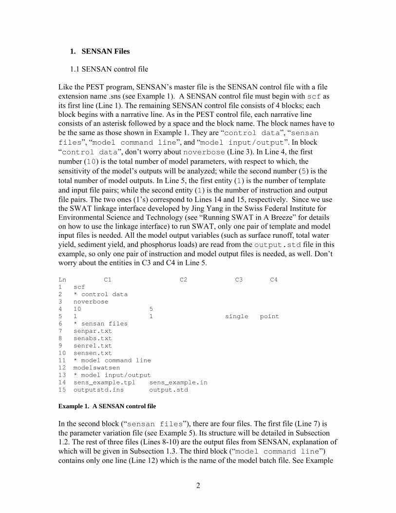
1.1 SENSAN control file Like the PEST program, SENSAN’s master file is the SENSAN control file with a file extension name .sns (see Example 1). A SENSAN control file must begin with scf as its first line (Line 1). The remaining SENSAN control file consists of 4 blocks; each block begins with a narrative line. As in the PEST control file, each narrative line consists of an asterisk followed by a space and the block name. The block names have to be the same as those shown in Example 1. They are “control data”, “sensan files”, “model command line”, and “model input/output”. In block “control data”, don’t worry about noverbose (Line 3). In Line 4, the first number (10) is the total number of model parameters, with respect to which, the sensitivity of the model’s outputs will be analyzed; while the second number (5) is the total number of model outputs. In Line 5, the first entity (1) is the number of template and input file pairs; while the second entity (1) is the number of instruction and output file pairs. The two ones (1’s) correspond to Lines 14 and 15, respectively. Since we use the SWAT linkage interface developed by Jing Yang in the Swiss Federal Institute for Environmental Science and Technology (see “Running SWAT in A Breeze” for details on how to use the linkage interface) to run SWAT, only one pair of template and model input files is needed. All the model output variables (such as surface runoff, total water yield, sediment yield, and phosphorus loads) are read from the output.std file in this example, so only one pair of instruction and model output files is needed, as well. Don’t worry about the entities in C3 and C4 in Line 5. Ln C1 C2 C3 C4 1 scf 2 * control data 3 noverbose 4 10 5 5 1 1 single point 6 * sensan files 7 senpar.txt 8 senabs.txt 9 senrel.txt 10 sensen.txt 11 * model command line 12 modelswatsen 13 * model input/output 14 sens_example.tpl sens_example.in 15 outputstd.ins output.std Example 1. A SENSAN control file In the second block (“sensan files”), there are four files. The first file (Line 7) is the parameter variation file (see Example 5). Its structure will be detailed in Subsection 1.2. The rest of three files (Lines 8-10) are the output files from SENSAN, explanation of which will be given in Subsection 1.3. The third block (“model command line”) contains only one line (Line 12) which is the name of the model batch file. See Example

2

2. The last block (“model input/output”) contains the pair(s) of template-input file and pair(s) of instruction-output file. A typical template file is given in Example 3; while the instruction file for reading output.std file is given in Example 4. Details about model batch file, template and instruction files are given in another note entitled “Getting Started with PEST”. @ echo off sw_edit > nul swat2000 > nul Example 2. The model batch file ptf $ v__SURLAG.bsn $surlag $ v__CN2.mgt $cn2f $ v__ESCO.hru $esco $ v__ALPHA_BF.gw $alpha_bf $ v__SLOPE.hru $slope $ v__SPEXP.bsn $spexp $ v__PHOSKD.bsn $phoskd $ v__PSP.bsn $psp $ v__SOL_SOLP.chm $sol_solp $ v__SOL_ORGP.chm $sol_orgp $ Example 3. A typical template file when using the SWAT linkage interface pif $ $AVE ANNUAL BASIN VALUES$ l6 $=$ !runoff! l7 $=$ !wtryld! l5 $=$ !sedyld! $NUTRIENTS$ l2 $=$ !orgpyld! l3 $=$ !solpyld! Example 4. A typical instruction file for reading output.std

1.2 Parameter variation file SENSAN’s task is to run a model as many times as a user requires, providing the model with a user-specified set of parameter values on each occasion. The parameters which are to be varied from model run to model run are identified on one or a number of template files. The values which these parameters must take on successive model runs are provided to SENSAN in a “parameter variation file”, an example of which is presented in Example 5. The file shown in Example 5 provides 11 sets of values for 10 SWAT parameters; the parameter names appear in Line 1. The same parameter names must be cited on template file(s) provided to SENSAN. The second line (Line 2) contains the nominal value for each parameter, that is, the “control” scenario. In the third line, the value for parameter

3

SURLAGE increases by 5% while the rest 9 parameters remain constant at their nominal values. In the fourth line, the value for parameter CN2F increases (or decreases) by 5% while the remaining 9 parameters (including SURLAG) take their nominal values, and so forth. A separate SWAT run will be undertaken for each row. The results, printed in the output.std file for each SWAT run, will be read through the instruction file (Example 4) by SENSAN, which will conduct some simple calculations and export these results to the three SENSAN output files (see Lines 8-10 in Example 1). 1 SURLAG CN2F ESCO ALPHA_BF SLOPE SPEXP PHOSKD PSP SOL_SOLP SOL_ORGP

2 4 73 0.95 0.021 0.1 1.5 90 0.24 15 125

3 4.2 73 0.95 0.021 0.1 1.5 90 0.24 15 125

4 4 76.65 0.95 0.021 0.1 1.5 90 0.24 15 125

5 4 73 0.9975 0.021 0.1 1.5 90 0.24 15 125

6 4 73 0.95 0.02205 0.1 1.5 90 0.24 15 125

7 4 73 0.95 0.021 0.105 1.5 90 0.24 15 125

8 4 73 0.95 0.021 0.1 1.575 90 0.24 15 125

9 4 73 0.95 0.021 0.1 1.5 94.5 0.24 15 125

10 4 73 0.95 0.021 0.1 1.5 90 0.252 15 125

11 4 73 0.95 0.021 0.1 1.5 90 0.24 15.75 125

12 4 73 0.95 0.021 0.1 1.5 90 0.24 15 131.25

Example 5. A parameter variation file (The numbers in the most left column are line labels; they are not contained in the real file)

1.3 SENSAN output files SENSAN produces three output files (named “senabs.txt”, “senrel.txt”, and “sensen.txt”), each of which is easily imported into a spreadsheet for subsequent analysis. In each of these files the first 10 (or the number of varying parameters) columns contain the parameter values supplied to SENSAN in the parameter variation file. The subsequent 5 (or the number of model output variables of interest) columns pertain to the 5 model output variables cited in the instruction file supplied to SENSAN. The first row of each of these output files contains parameter and observation names. These three files differ from each other only by the values provided (calculated) in the last 5 columns for the model output variables. The last 5 entries on each line of the first output file (senabs.txt) simply list the 5 model outputs read from the model output file (output.std) after the model was run using the parameter values supplied as the first 10 entries of the same line. An example of the senabs.txt file is presented in Example 6. The first three columns (C1-C3) are (omitted) parameter values while the last 5 columns (C4-C8) are values for surface runoff (RUNOFF), total water yield (WTRYLD), sediment yield (SEDYLD), organic P yield (ORGPYLD), and soluble P yield (SOLPYLD). The second SENSAN output file (senrel.txt) lists the relative difference between model output values on second and subsequent data lines of the first output file (senabs.txt) and model output values cited on the first data line. We don’t need this

4

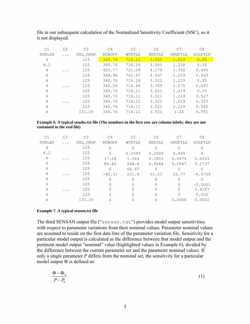
file in our subsequent calculation of the Normalized Sensitivity Coefficient (NSC), so it is not displayed.

C1 C2 C3 C4 C5 C6 C7 C8 SURLAG ... SOL_ORGP RUNOFF WTRYLD SEDYLD ORGPYLD SOLPYLD

4 125 340.76 716.11 3.521 1.219 0.55 4.2 125 340.76 716.16 3.561 1.228 0.55 4 ... 125 403.77 721.09 4.179 1.392 0.646 4 125 344.96 741.97 3.567 1.233 0.563 4 125 340.76 716.18 3.521 1.219 0.55 4 ... 125 340.54 716.64 3.789 1.275 0.547 4 125 340.76 716.11 3.521 1.219 0.55 4 125 340.76 716.11 3.521 1.219 0.527 4 ... 125 340.76 716.11 3.521 1.219 0.555 4 125 340.76 716.11 3.521 1.219 0.565 4 131.25 340.76 716.11 3.521 1.26 0.551

Example 6. A typical senabs.txt file (The numbers in the first row are column labels; they are not contained in the real file)

C1 C2 C3 C4 C5 C6 C7 C8 SURLAG ... SOL_ORGP RUNOFF WTRYLD SEDYLD ORGPYLD SOLPYLD

4 125 0 0 0 0 0 4.2 125 0 0.2499 0.2000 0.045 0 4 ... 125 17.26 1.364 0.1803 0.0474 0.0263 4 125 88.42 544.4 0.9684 0.2947 0.2737 4 125 0 66.67 0 0 0 4 ... 125 -42.31 101.9 51.53 10.77 -0.5769 4 125 0 0 0 0 0 4 125 0 0 0 0 -0.0051 4 ... 125 0 0 0 0 0.4167 4 125 0 0 0 0 0.020 4 131.25 0 0 0 0.0066 0.0002

Example 7. A typical sensen.txt file The third SENSAN output file (“sensen.txt”) provides model output sensitivities with respect to parameter variations from their nominal values. Parameter nominal values are assumed to reside on the first data line of the parameter variation file. Sensitivity for a particular model output is calculated as the difference between that model output and the pertinent model output “nominal” value (highlighted values in Example 6), divided by the difference between the current parameter set and the parameter nominal values. If only a single parameter P differs from the nominal set, the sensitivity for a particular model output Ф is defined as:

0

0P PΦ−Φ−

(1)

5

Where Ф0 and P0 are model output and parameter nominal values and Ф and P are the model output and parameter values pertaining to a particular model run. An example of the sensen.txt file is presented in Example 7.

2. Calculating Normalized Sensitivity Coefficient (NSC) Using MS Excel The normalized sensitivity coefficient (or sensitivity index) is calculated through the following formula:

0 0 0

0 0 0

( ) /( ) /

PNSCP P P P PΦ −Φ Φ Φ −Φ

= =− −

0

0

×Φ

(2)

Or

0 0

0 0

| || |PNSC

P PΦ −Φ

= ×− Φ

(3)

Where, the NSC is a dimensionless positive number, whose value indicates the relative importance of parameter P on the model output Ф, that is, the relative sensitivity of the particular model output Ф with respect to the changing of the particular model parameter P. The following steps illustrate how to calculate the NSC’s from the two SENSAN output files (senabs.txt and sensen.txt) using MS Excel. Step 1: Create a new spreadsheet file named the current worksheet as surface runoff.

6

Step 2: Using MS Excel File Import Wizard to open the senabs.txt file and copy the 10 parameter names and their nominal values.

Step 3: Place cursor in Cell A2 of surface runoff; right click and select Paste Special … on the pop-up menu; and check the box in front of Transpose.

7

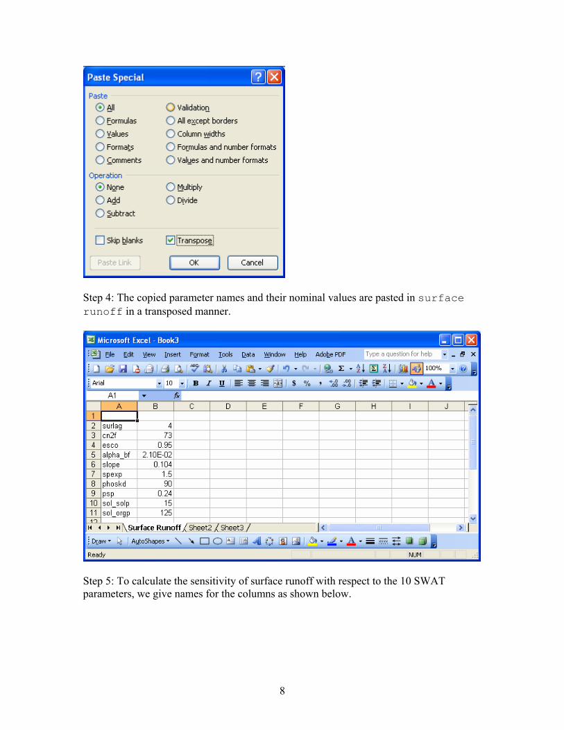
Step 4: The copied parameter names and their nominal values are pasted in surface runoff in a transposed manner.

Step 5: To calculate the sensitivity of surface runoff with respect to the 10 SWAT parameters, we give names for the columns as shown below.

8

Step 6: From senabs.txt file we copy the “nominal” value of surface runoff (340.76 mm).

9

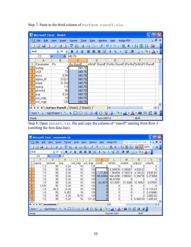
Step 7: Paste to the third column of surface runoff.xls.

Step 8: Open sensen.txt file and copy the column of “runoff” starting from Row 3 (omitting the first data line).

10

Step 9: Paste to surface runoff.xls.

Step 10: Calculate for surface runoff. 0 /P Φ0

11

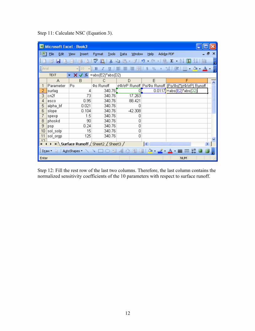
Step 11: Calculate NSC (Equation 3).

Step 12: Fill the rest row of the last two columns. Therefore, the last column contains the normalized sensitivity coefficients of the 10 parameters with respect to surface runoff.

12

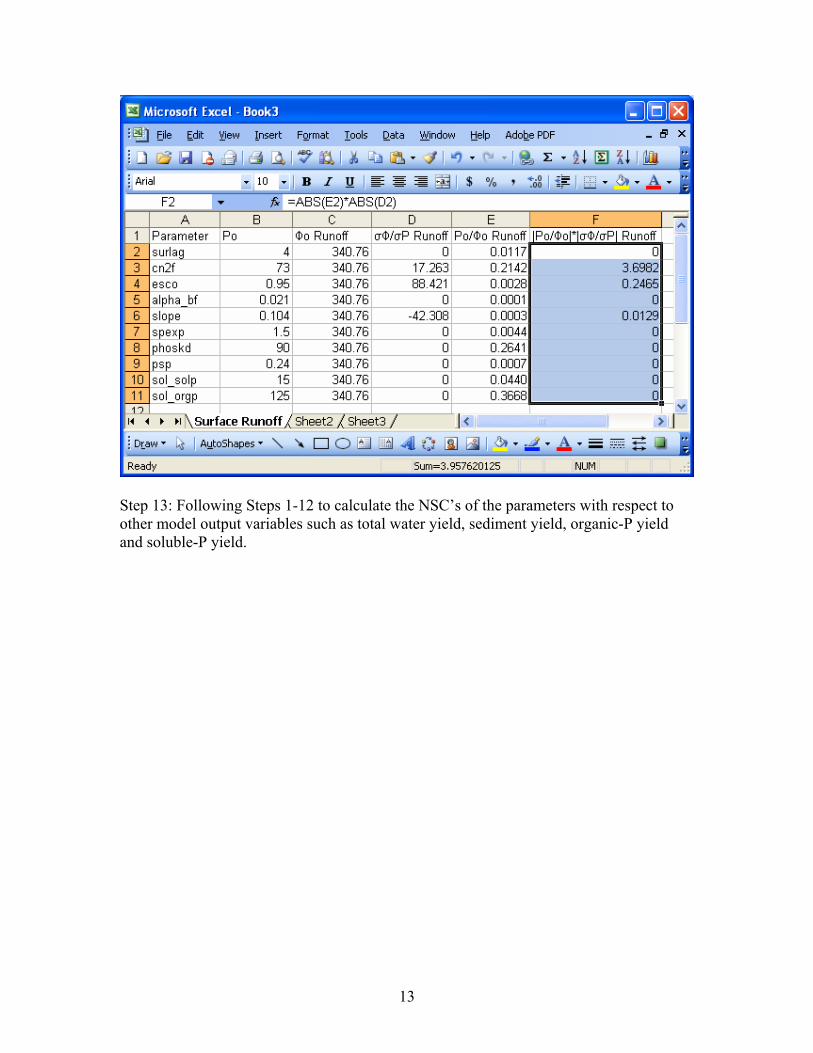
Step 13: Following Steps 1-12 to calculate the NSC’s of the parameters with respect to other model output variables such as total water yield, sediment yield, organic-P yield and soluble-P yield.

13