
Biometric Recognition Technologies and Biometric Applications

NISTIR 7855
Sensitivity Analysis for Biometric Systems A Methodology Based on Orthogonal
Experiment Designs
Yooyoung Lee James J Filliben Ross J Micheals
P Jonathon Phillips
httpdxdoiorg106028NISTIR7855
1
NISTIR 7855
Sensitivity Analysis for Biometric Systems A Methodology Based on Orthogonal
Experiment Designs
Yooyoung Lee Ross J Micheals
P Jonathon Phillips Information Access Division
Information Technology Laboratory
James J Filliben Statistical Engineering Division
Information Technology Laboratory
National Institute of Standards and Technology Gaithersburg MD 20899
httpdxdoiorg106028NISTIR7855
May 2012
US Department of Commerce John E Bryson Secretary
National Institute of Standards and Technology
Patrick D Gallagher Under Secretary for Standards and Technology and Director
2
Abstract
The purpose of this paper is to introduce an effective and structured methodology for carrying out a biometric system
sensitivity analysis The goal of sensitivity analysis is to provide the researcherdeveloper with the insight and
understanding of the key factorsmdashalgorithmic subject-based camera-based procedural image quality environmental
among othersmdashthat affect the matching performance of the biometric system under study This proposed methodology
consists of two steps 1) the design and execution of orthogonal fractional factorial experiment designs which allows the
scientist to efficiently investigate the effect of a large number of factorsmdashand interactionsmdashsimultaneously and 2) the use
of a select set of statistical data analysis graphical procedures which are fine-tuned to unambiguously highlight important
factors important interactions and locally-optimal settings We illustrate this methodology by application to a study of
VASIR (Video-based Automated System for Iris Recognition)mdashNIST iris-based biometric system In particular we
investigated k = 8 algorithmic factors from the VASIR system by constructing a ሺ2ଵ x 31 x 41) orthogonal fractional
factorial design generating the corresponding performance data and applying an appropriate set of analysis graphics to
determine the relative importance of the eight factors the relative importance of the 28 two-term interactions and the
local best-settings of the eight algorithms The results showed that VASIRrsquos performance was primarily driven by six
factors out of the eight along with four two-term interactions A virtue of our two-step methodology is that it is
systematic and general and hence may be applied with equal rigor and effectiveness to other biometric systems such as
fingerprints face voice DNA etc
Keywords sensitivity analysis iris recognition biometrics experiment design VASIR video-based biometric
system orthogonal fractional factorial characterization uncertainty factor effects interaction effects optimization main
effects plots interaction plots
1
1 Introduction
Biometrics is the study of identifying an individual based on human physiological or behavioral characteristics The
characteristics can include fingerprints face iris ocular area retina ear voice DNA signature gait and hand geometry
among others The use of biometrics has many advantagesmdashespecially as an attractive alternative to keys passwords
smartcards and other artifacts for physical entry In this regard biometric-based technologies are increasingly being
incorporated into specific security fields and applications such as industrial access control law-enforcement military
border control and forensics [1]
A significant problem in biometric studies is that researchersdevelopers often present results that lack an assessment
of intrinsic system uncertainty A high degree of input and output numerical precision often gives the impression of great
accuracy (and therefore confidence) but neglects to give attention to the critical questions of the sensitivity of the final
results to different algorithms environments subject characteristics and biometric sample conditions [2] Hornberger and
Spear [3] made the following paraphrased statement about simulation models Most such models are complex with many
parameters state-variables and underlying non-linear relations under optimal circumstances such systems have many
degrees of freedom andmdashwith judicious adjustmentsmdashare susceptible to over-fitting in which they can be made to
produce virtually any desired behavior often with both plausible structure and ldquoreasonablerdquo parameter values We believe
that the above statement applies equally well for biometric systems
Sensitivity analysis is the study of how the output of a system is affected by different inputs to the system [4] while
optimization analysis is the determination of system parameter settings that yield the best system performance In essence
a biometric system is a data monitoring and decision-making ldquomachinerdquo A good biometric system has a high proportion
of correct decisions All biometric systems are susceptible to incorrect decisionsmdashespecially in the presence of less-than-
optimal conditions
In practice the performance of many biometric systems is frequently examined and optimized via a series of one-
factor-at-a-time experiment designs in which most factors in the system are held constant while one factor is focused on
and varied to examine its effect This design though popular [56] has the disadvantage that it can yield grossly biased
(incorrect) estimates of factor effects Further this design has no capacity to estimate factor interactionsmdashwhich are
intrinsic to many biometric systems
This is the motivation to introduce to the biometrics community an alternative method for conducting a sensitivity
analysis We demonstrate the method on the VASIR iris recognition system to yield more accurate and reliable results
with the advantage that
1) The system is better understood
2) The system is better characterized
3) The system is better optimizedmdashwith the effect that system performance is significantly improved in a
computationally efficient fashion
2
Thus in short the objective of this paper is to introduce and apply a structured ldquoSensitivity Analysisrdquo approach for
gaining insight and understanding about the systemrsquos key components those which affect the quality and performance of
a biometric system and to optimize the settings of these key components
Sensitivity analysis as we describe it has two separate and distinct steps
1) Experiment Design (the structured plan for collecting the data) and
2) Statistical Analysis (the structured methodology for analyzing the data)
Both parts are critical and when optimally used in concert yield enhanced insight into the relative importance and
effect of the various computational components (and interactions) affecting biometric system performance The
experiment design and data analysis are demonstrated by a particular iris-based biometric system VASIR (Video-based
Automated System for Iris Recognition) which has verification capability for both traditional still iris images and video
sequences captured at a distance while a person walks through a portal [7]
The general structure of this paper is three-fold
1) Orthogonal fractional factorial design Introduce to the biometrics community a structured orthogonal
fractional factorial experiment design methodology to efficiently gain insight and understanding (ldquosensitivity
analysisrdquo) of critical system parameters interactions and their optimal settingsmdashthis introduces and applies
an established method within the statistical community [89]
2) Sensitivity analysis Present effective and insightful statistical analysis methodologies for carrying out
sensitivity studies
3) Demonstration with VASIR Demonstrate our experiment design and analysis methodologies for VASIR
with potential application to the broader biometrics field
This sensitivity analysis approach provides a tool for understanding the computational components affecting the
overall performance of a biometric system Based on such understanding the logical follow-up is to carry out an
optimization analysis (identifying the optimal global settings of the components) and a robustness analysis (assessing the
range of validity for our sensitivity and optimization conclusions) Our current paper focuses on the details of the
sensitivity analysis only To demonstrate the elements of the sensitivity analysis approach we restrict our focus to a fixed
setting for two robustness factors 1) eye position (left eye only) and 2) image type (video matching non-ideal to non-
ideal image only)
2 Sensitivity Analysis Methodology
Sensitivity analysis is the experimental process by which we determine the relative importance of the various factors
of a system Suppose a system has k factors (input parameters) which potentially affect its performance The minimal
deliverable of a sensitivity analysis is to produce a ranked list of those k factorsmdashordered most to least important For
complicated systems (eg biometrics) a more desirable deliverable is to produce a ranked list which contains not only
the k main factors but also includes the various interactions of a system To generate such a list implicitly means that each
factor effect must be estimable and such estimates should have as small as possible bias and sampling uncertainty 3
As it turns out such minimal bias and uncertainty is driven primarily by the choice of experiment design that the
analyst employsmdashsome designs yield noisy effect estimates while others yield very accurate estimates
A good experiment design is importantmdashit assures that the resulting data from the design has the capacity to answer
the scientific question at handmdashin particular the data must have the capacity to yield a valid and rigorous ranking of the
factors under study Important as the experiment design component is a complementary component is also important
namely the statistical analysis methodology employed to analyze the data resulting from the designmdashwhat techniques
must be brought to bear on the data so as to optimally estimate order and highlight the various factor effects Hence
sensitivity analysis consists of two separate and distinct steps
1) Experiment Design (the structured plan for collecting the data) and
2) Statistical Analysis (the structured methodology for analyzing the data)
Both parts are important and when optimally used in concert they yield copious insight into the relative importance
of the various computational components (and interactions) that affect biometric system performance The detailed
elements of the two components for our sensitivity analysis are illustrated by application to a particular iris-based
biometric system VASIR (Video-based Automated System for Iris Recognition) which has verification capabilities not
only for traditional still iris images but also for video sequences taken at a distance (see the details in Section 3)
21 Experiment Design
Experiment design as a discipline is a systematic rigorous approach for scientific and engineering problem-solving
The general goal of experiment design is three-fold
1) to produce insight and understanding into the factorial dependencies of a system
2) to produce unambiguous valid and defensible conclusions
3) to achieve both of the above with as small a sample size (time and cost) as possible [10]
Sensitivity Analysis offers to the biometric scientist the understanding and insight as to what is important and what is
not in a systemmdashand where the scientist should focus near-term and long-term research efforts In this regard we shall
review and compare four commonly used experiment designs for sensitivity analysis 1) Randomization Designs (Monte
Carlo) 2) One-Factor-at-a-time (1FAT) Designs 3) Full Factorial Designs and 4) Orthogonal Fractional Factorial
Designs
1) Randomization Designs (Monte Carlo)
Monte Carlo is a common methodology for many scientific sensitivity analysis studies In essence it
considers the entire population space of factors and settings and then randomly samples a user-specified
number from that population space (see details in Kleijnen [11]) The advantage of Monte Carlo is that ldquoon
the averagerdquo the estimated main effects and the interactions will be unbiased The primary disadvantage with
Monte Carlo is that it tends to be expensive the required sample size to estimate factor effect of the desired
precision frequently exceeds an affordable sample size
2) One-Factorndashat-a-Time (1FAT) Designs
4
1FAT is an extremely common and popular sensitivity analysis methodology in both the biometric
community and the larger scientific community In the 1FAT design an initial run is made where all k factors
are set at a baseline value and k subsequent runs are made whereby each factor in succession is changed to an
alternative value 1FAT designs are simple intuitive and inexpensive (costing as little as n = 1+k runs) On
the other hand we will demonstrate below that such designs routinely produce effect estimates (and hence
the subsequent ranked list of factors) which can be significantly biased and imprecise (see Box et al [12] and
Saltelli et al [4]) Further 1FAT designs have no ability whatsoever to estimate interactionsmdashwhich are quite
common in biometric systems Of course such interactions will make themselves evident by contaminating
(biasing) the one thing that 1FAT designs do producemdashestimates of the k main factors
3) Full Factorial Designs
Full factorial designs consist of running all possible combinations of all levels of all factors (see details in the
NIST website [10]) The advantage of a full factorial design is that it is information-richmdashsuch a design will
provide rigorous information (estimates) about the relative importance of all k main factors and all
interactions (2-term 3-term hellip k-term) Given these estimates it is thus an easy step to generate the ideal
ranked list which includes all main effects and all interactions of all orders In terms of information content
it is difficult to go wrong with a full factorial design On the other hand the significant disadvantage of full
factorial designs (which prevents its widespread use for large-k systems) is that such designs are frequently
k factors have if all ൌ 2levels the total cost is ൌ 2k factors have too expensive For example if all
k the resulting n can quickly and hence even for modest values of ൌ 3levels the total cost is ൌ 3
become unaffordableexpensive
4) Orthogonal Fractional Factorial Designs
Orthogonal Fractional Factorial Designs are a viable alternative to full factorial designs because they use only
a fraction of the runs needed for a full factorial design while still yielding good effect estimates (see details
on the NIST website [10]) Designs with both 1- and 2-dimensional balance are referred to as ldquoorthogonal
designsrdquo which is balanced for every single factor in the design and balanced for every pair of factors in the
design respectively Balanced for a single factor means that every setting in that factor occurs the same
number of times in the n runs Balanced for a pair of factors means that every possible pair of settings across
the two factors occurs the same number of times in the n runs Note that for a k-factor design to be orthogonal
the design must have 1-dimensional balance for each (and every) one of the k factors under study and must
have 2-dimensional balance for each (and every) one of the ൫ଶ൯ combinatorial pairs of factors in the design
As an example for the simplest case in which each of k factors has only two levels then for an n-run
experiment a factor is singly-balanced if the two levels (eg -1 and +1) occur the same number of times (=
n2) across the n runs Similarly two factors with two levels are doubly-balanced if the four combinations (-
1-1) (+1 -1) (-1 +1) and (+1 +1) occur the same number of times (= n4) across the n runs The primary
5
virtue of orthogonal designs is that their balance yields excellent (small bias and high precision) statistical
estimates for the main effects and interactions
We note in passing that full factorial designsmdashthough typically expensivemdashare inherently orthogonal To retain the
estimation virtues of orthogonality while avoiding the run-expense of full factorial designs leads one to consider the use
of orthogonal fractional factorial designs Note that since a fractional factorial design is any design whose total number of
runs n is less than the corresponding full factorial design then by definition the 1FAT design is a fractional designmdashbut a
decidedly non-orthogonal fractional design and so has poor estimation properties
As alluded to above estimates from an orthogonal factorial design are far superior (unbiased and precise) to estimates
from the 1FAT design To demonstrate this we draw on an example from the chemical engineering industry where our
response variable of interest is percentage reacted (0 to 100 ) for an industrial chemical process [13] The k=5 factors
for this example are feed rate catalyst agitation rate temperature and concentration For simplicity these five factors
have only two levels The sensitivity analysis goal is the usual determine which of the five factors are most important in
affecting percentage reacted We carry out four separate sensitivity analyses of this k=5 chemical reaction processmdashusing
four different experiment designs Figure 1 shows these four designsmdashthree orthogonal designs and the 1FAT design
1)
2)
3)
mdashexpensiveൌ 32ሻ ହ2Two-level orthogonal full factorial design (
mdashhalf expensive ൌ 16ሻ ହଵ2Two-level orthogonal fractional factorial design (
mdashinexpensive and ൌ 8ሻ ହଶ2Two-level orthogonal fractional factorial design (
4) Two-level 1-Factor-at-A-Time (1FAT) design ሺ ൌ 6ሻmdashinexpensive
Note that one might argue that 1FAT designs are poor due to the smaller number of runs This however is not the case
as may be seen by the 2ହଶ orthogonal designmdashconsisting of a similar small number of runs (8)mdashand yet having vastly
superior estimation properties over the 1FAT The left-most column in Figure 1 has the name of the design and the
number of runs (n = 32 16 8 and 6 respectively) The second-left panel has the corresponding experimental design
matrix (details omitted) along with a response column ldquoYrdquo resulting from a behind-the-scenes simulation model with
known factor and interaction coefficients (see details in the book written by Box et al [13]) Given the generic sensitivity
analysis question determine the most important factors in this k=5 factor experimentrdquo the rightmost panel gives the
ldquoanswerrdquomdashthe ranked list that results after the design data collection and data analysis Note that the behind-the-scenes
simulation model had the property that the most important factor was X2 (with an effect size of 195) followed by the
next most important factor (a 2-term X2X4 interaction with value 1325) etc We assess the relative merit of the four
designs by comparing their resulting ranked list estimates with this known ground truth (Bଶ ൌ 195 Bଶସ ൌ 1325 hellip ሻ
6
Figure 1 Comparison of three orthogonal designs and the 1FAT design determining the most important factors out
of five factors
In particular we can go to the top of the four ranked lists and extract the ldquomost important factorrdquo as estimated by each
of the four particular experiment designs and compare it with the known truth In doing so we see that
1) The expensive (n=32) 2ହ full factorial design identified factor X2 as its most important factor with an
estimated effect size of Βଶ ൌ 195 this was identical to the Bଶ ൌ 195 coefficient in the underlying
simulation function
2) The half-as-expensive (n=16) 2ହଵ orthogonal fractional factorial design also determined X2 as the most
important factor and estimated its effect as Βଶ ൌ 205mdashclose to 195 but with only half the experimental
expenseeffort
3) The inexpensive (n=8) 2ହଶ orthogonal fractional factorial design also chose X2 as the most important factor
and estimated its effect as Βଶ ൌ 2025mdashalso close (but with an issue of confounding with the X1X4 effect
which must be examined)
4) On the other hand the least expensive (n=6) 1FAT fractional factorial design determined (incorrectly) that
X1 was the most important factor andmdasheven worsemdashfound that X2 was the least important factor with its
estimated effect being only Βଶ ൌ 20mdashincorrect (biased) by an order of magnitude from the truth
7
The two-level orthogonal fractional factorial designs were remarkably accurate insightful and extremely efficient
while the 1FAT design yielded grossly biased estimates and incorrect sensitivity analysis conclusions The above
illustration is not necessarily the exception In a scientificbiometric experimental situation if the performance response
function has any interactions whatsoever then orthogonal fractional factorial designs typically yield excellent trusted
sensitivity analysis conclusions while 1FAT designs typically yield incorrect and skewed conclusions Our proposed
sensitivity analysis approach acknowledges this superiority and thus uses orthogonal fractional factorial designs as the
centerpiece for its experiment design component
22 Data Analysis
For the analysis of data drawn from orthogonal fractional factorial designs the available statistical methods fall into
two broad categories 1) quantitative and 2) graphical For quantitative methods there are a variety of tools that could be
employed (see Box et al [12]) with the classical ANOVA (Analysis of Variance) method being the most common
quantitative tool for sensitivity analysis On the other hand these quantitative methods are not always the best practical
choice for the analysis of sensitivity experiments for a variety of reasons too much of a ldquoblack boxrdquo of statistical
procedures too much of a removal from the raw data too many assumptions which must be adhered to and tested for and
too much of a loss of feeling as to whether the resulting conclusions are consistent with the data
For this reason we find that a superior (in regard to maximizing insight) approach to the analysis of data from
sensitivity experiments is via graphical data analysis methodsmdashin particular EDA (Exploratory Data Analysis) graphical
methods Such methods take the approach of keeping ldquoclose tordquo the data and judiciously displaying the data in such a
fashion that the relative importance of the factors (and interactions) becomes evident from the (judiciously constructed
and augmented) plots In this regard we have constructed a battery of graphical procedures fine-tuned for sensitivity
studies conducted via orthogonal (full or fractional) experiment designs This battery of procedures was developed at
NIST [81415] and is an integral part of the NIST-developed analysis tool Dataplot [1416]
The battery consists of the following ten graphical procedures 1) Ordered Data plots 2) Dex (design of experiment)
Scatter plots 3) Main Effects plots 4) Dex Interaction Effects Matrix 5) Block plots 6) Dex Youden plots 7) Effects
plots 8) Half-normal Probability plots 9) Cumulative Residual Standard plots and 10) Contour plots A full application
of all ten of these graphical tools for this biometrics example is unneeded here and is beyond the scope of this papermdashit
will suffice for us to demonstrate the power of the Sensitivity Analysis methodology to utilize three of the ten tools 1) the
Ordered Data plot 2) the Main Effects plot and 3) the Interaction Effects Matrix These graphical data analysis methods
serve as an important post-data component which complements the pre-data orthogonal experiment design component
3 VASIR (Video-based Automatic System for Iris Recognition)
Iris recognition is a popular biometric system approach whose effectiveness is due to the highly distinctive features of
the human iris Most commercial systems for iris recognition are relatively expensive and are computational black boxes
that run proprietary algorithms In this light to advance iris-based biometrics technologymdashIrisBEE (Iris Biometric 8
Evaluation Environment) [17] algorithmmdashwas implemented in the C programming language from Masekrsquos Matlab code
[5] IrisBEE was developed as a baseline for traditional still-based iris recognition and hence there is still a need to
overcome a number of challenges for images taken under more flexible acquisition and environmental condition (eg
video taken at a distance)
In contrast to IrisBEE VASIR [718] was developed with Near-Infrared (NIR) face-visible video-based iris
recognition as part of its domain scope VASIR is a fully automated system for video-based iris recognition capable of
handling videos that were captured under less-constrained environmental conditions such as a person walking through a
portal at a distance The VASIR system was designed developed and optimized to be robustmdashto address the challenge of
recognizing a person in less-than-optimal environments while coping with both high and low imagevideo quality Unlike
commercial iris recognition software (expensive and black box) VASIR provides an opportunity for the biometrics
research community to examine the effect of algorithmic component changes to extract and re-use its freely available
source code and to otherwise advance the state-of-the art of iris recognition technology
Although VASIR was developed with less-constrained video-based iris recognition in mind VASIR also robustly
accommodates the constrained still-based iris recognition VASIR supports multiple matching scenarios
1) Video (at a distance) to Video (at a distance) (VV)
2) Video (at a distance) to Still (classical) (VS) and
3) Still (classical) to Still (classical) (SS) iris recognition
In VV matching the extracted iris region from video frames is matched to other frames from the same video or to
frames from a different video sequence of the same person VS means that the video captured at a distance is compared to
classical still images captured by a different device SS matching is a traditional iris recognition scenario in which a
classical still-image is matched against other classical still-images of the same person that were captured by the same (or
similar) device
VASIR has the capacity to automatically detect and extract the eye region and subsequently to automatically assess
and select the best quality iris image from NIR face-visible video After this process VASIR carries out a comprehensive
image comparison analysis that in turn yields a verification result As shown in Figure 2 the VASIR system can
principally be categorized into three modules 1) image acquisition 2) video processing and 3) iris recognition
9
Figure 2 VASIR system architecture
Each module consists of several components that have all been designed developed and optimized to achieve high
verification performance In the Image Acquisition module VASIR loads a still image or video sequence In the Video
Processing module VASIR automatically detects the eye region from facehairshoulder visible frames in a video
sequence and extracts the leftright iris images VASIR then calculates automatically the image quality score of the
extracted iris image from each frame Based on the quality score the best quality iris imagesmdashone for left and one for
rightmdashare automatically chosen from all available frames The Iris Recognition module is fed either the resulting iris
images from the Video Processing module or the still iris image For both video and still iris images VASIR localizes the
iris region based on the results of the segmentation algorithm The segmented iris regions are then extracted and
normalized based on polar coordinates and interpolation Next VASIR extracts the features from the normalized iris
images and encodes the extracted features as binary strings along with a noise-mask In the matching stage VASIR
matches the extracted biometric template to existing templates Note that all procedures are fully automaticmdashsee Leersquos
paper [7] for detailed methods and procedures
4 Experiment Design VASIR Case
The purpose of a Sensitivity Analysis is first and foremost to gain insight into the important factors (and interactions)
which drive the biometrics system In this regard the primary Sensitivity Analysis output is a ranked list of factors and
10
interactions along with estimates of the magnitude of their effects To achieve that the biometrics researcher needs to
provide information about the following 1) model 2) factors 3) responses 4) max affordable number of runs and 5)
choice of design
41 Model
The starting point for a formal experiment design is to represent a model for the system response For many scientific
applications a generic response model can be expressed as
ሻhellip ଶ ଵሺ ൌ
where Y represents a general response and k represents the number of factors that affect the response
In the case where we have multiple responses as in VASIR the model can be generalized to
ሻhellip ଶ ଵሺൌ
to indicate that the different factors may affect each individual response Y୧ in its own and separate way
42 Factors
For a biometric system in general there are many factors (parameters or variables) that can affect a systemrsquos response
(or performance)mdashthe VASIR system is no exception The VASIR factors naturally fall into four categories 1)
environmental conditions 2) image conditions 3) subject characteristics and 4) algorithmic components Factors
described in Table 1 are 33 factors from the first three categories which could be examined unto themselves to assess the
robustness of our algorithmic conclusions
Table 1 Possible robustness factors that affect a biometric system
Environmental conditions Image conditions Subject characteristics
1) indooroutdoor 7) focus or sharpness 18) contact lenses 2) lighting 8) contrast 19) glasses 3) background 9) brightness 20) leftright 4) weather 10) motion blur 21) gender 5) camera 11) resolution 22) age 6) daynight 12) noise
13) color 14) distortion 15) artifacts 16) reflections 17) video still
(scenarios)
23) cosmetics (eg mascara) 24) hair color 25) race 26) movement 27) distance from camera 28) skin color 29) eye color 30) eyelashes 31) eyebrows 32) pupil dilation 33) usability (eg behavior
training perception)
11
Table 2 illustrates a list of 38 algorithmic factors (VASIR-specific) which potentially affect VASIR performance
Table 2 VASIR possible algorithmic factors and their popular settings that can be controlled for optimization
Key components Possible parametersmethodsfactors Type Popular settings Settings
Image acquisition (IA) Image quality control D Quality control system hellip 10
Eye region detection and
extraction (FX)
Algorithms D HaarPCA hellip 10 Classifier cascade types D eye-pair left-only righthellip 10 Minimum resolution for eye region C 0-200 200 Width of nose bridge C 1-100 100 X1 Pupil position alignment leftright D (on off) 2
Image quality Assessment
X2 Algorithms D Sobel LoG CONhellip 15 Image enhancementrestoration D Super-resolutionshellip 5
Best QualityImage Selection Algorithms D ABIShellip 3
Segmentation(SEG)
Pupil circle Algorithms D Hough active contours hellip 10 Datatype D Video still iris webcam 5 Ratio between width and height C 1-12 12 Thresholds C 0-255 256 Scale C 1-4 5 Radius limits C 1-200 200 Closing iterations C 0-4 5 Opening iterations C 0-4 5 Iris circle Algorithms D Hough active contours hellip 10 Datatype D Video still iris webcam 5 Thresholds C 0-1 (0102hellip) 100 Scale C 1-4 5 Radius limits C 1-200 200 Distance between pupil c and iris c C 1-100 100 Eyelids
X3 Algorithms D linecurve fitting hellip 10 Adjustment C 0-9 10 Noise removal Thresholding for eyelashes C 0-19 20 Thresholding for reflections C 235-255 20
Normalization (NORM)
Algorithms D Polar interpolations 4 X4 Radial resolution C 1-100 100 Angular resolution C 1-500 500
Feature extraction and
encoding(FX)
Algorithms D Gabor SIFT DAISY hellip 10 Gabor-wavelet parameters X5 Wavelength (pixel unit) C 1-30 30 Bandwidth C 0-1 100 X6 Masking a level of magnitudes C (0-5) (80-100) 25 Encoding scale C 1-10 10
Similarity metrics (SM)
X7 Algorithms D Hamming L2 COShellip 10 Directional bit-wise shifting method X8 Horizontal ( left and right) C 0-29 30 Vertical (Up and down) C 0-9 10
Type C = Continuousquantitativeordinal D = Discretequalitativenon-ordinal)
At a minimum an experiment design is characterized by two numbers (k n) where k is the number of factors in our
study and n is the affordable number of runs If we chose to examine and vary all of the factors listed in Table 1 and Table
2 k would equal 71 (=33+38) In general the number of runs n must exceed the number of factors k to obtain estimates
12
This is too expensive for our time 2500 two-term interactions this would require ൯ଶ൫=71 factors and the for the k
and cost constraints Inasmuch as the purpose of our study is to demonstrate the efficiency of our experiment design
technique and to understand and optimize the algorithmic factors of VASIR we thus choose to focus primarily on only the
eight specific algorithmic factors
An important early step in the structured experiment design process was to collect and construct a superset of possible
variables (ldquofactorsrdquo) that may affect the quality and performance of the VASIR algorithmmdashthis led to the 38 factors in
this category For this study if we analyzed all 38 algorithmic factors this would require gt 750 observationsmdashstill too
expensive
To accommodate affordability the second step was to reduce the number of factors k We hence choose to limit
ourselves to only k=8 algorithmic factors (one or two factors from each of the eight key components in Table 2) we
highlighted these eight algorithmic factors in Table 2 with gray The reason why we have chosen these eight algorithmic
factors is so that at least one factor was varied for each VASIR key component (excepting the Best Image Quality
Selection component whose setting is dictated by the choice utilized for preceeding Image Quality Assessment
component) Other reasons for our choice of these eight algorithmic factors were to analyze the sensitivity of new
methods being considered for VASIR to focus on those methods of greatest research interest and to concentrate on those
specific algorithms for recent upgrades for VASIR
As a next step we reduced the number of setting levels of the eight algorithmic factors Table 3 summarizes the eight
chosen algorithmic factors and their setting levels
Table 3 The eight algorithmic factors and their setting levels (see detailed procedures in the paper [7])
Eight algorithmic factors Number of setting levels
X1 (EyeAlg) Eye position alignment -1
(OFF)
+1
(ON)
X2 (IQMetr) Image quality metrics -1
(SOB)
0
(LoG)
+1
(CON)
X3 (SegEye)Eyelids segmentation -1
(Lines)
+1
(Curves)
X4 (NorRes) Radial resolution -1
(20px)
+1
(32px)
X5 (FXWL) Wavelength -1
(18px)
+1
(16px)
X6 (FXMask) Wavelet magnitude -1
(08)
+1
(09)
X7 (SMAlg) Similarity metrics -2
(HD)
-1
(COR)
+1
(COS)
+2
(WED)
X8 (SMSh) Horizontal shifting -1
(10)
+1
(5)
13
The detailed methods for each factor are described as follows
1) X1 (EyeAlg) Eye position alignment
A tilted head or subject movement results in a larger angular difference between the target and the query iris
imagemdashcausing rotational inconsistency ie the matching point within the two iris templates is different In
VASIR to compensate for the angular difference the positions of the left and right eyes were automatically
and angularly aligned according to the estimated degree of the distance difference of the left and right pupil
center We analyzed whether the eye position alignment approach (ON) was actually better than without eye
position alignment (OFF)
2) X2 (IQMetr) Image quality metrics
The image quality assessment can help to predict whether an image is usable or recognizable and it can also
help to determine which image out of a set of frames in a video sequence has the best quality VASIR
developed multiple quality metrics for measuring iris image quality automatically for images (or videos)
captured in different environments VASIR automatically selects the best quality iris frame out of a video on
the quality assessment metric Although 16 metrics [7] were introduced to measure one or another aspect of
image quality we focused on the following three metrics (SOB LoG CON) for our sensitivity analysis
A Sobel (SOB) filter
The Sobel operator has been used extensively for image edge detection and for measuring the focus
level of an image [192021] The gradient at each point and the orientation of that gradient (gradient
magnitude) can be measured by
ଶݕሺݔ ܦ ሻሻݕ ሺ ଶݔሺݔ ܤ ሺඥൌܦ ሻሻݕ
These filters ሻrightሺܦݕ andሻleftሺ ݔܦ filters defined as 3 ൈ 3The Sobel operator consists of a pair of
are designed to respond to edges running vertically and horizontally relative to the pixel grid
B Laplacian of Gaussian (LoG) filter
LoG is an important filter with much attention given to it [2223] LoG is defined as
ଶെ ߪ2 ଶ ݔଶݕൌ ܩܮ
ସߪ
We used a 9x9 filter with σ ൌ 14 in our experiment To measure the quality score the LoGED (Edge
Density) is computed as ெଵ ேଵ
eሺ௫మା௬మfraslଶఙమሻ
|
is the calculated value at LoGሺx yሻ is the number of pixels in the search area and ܯ ൈwhere
location ሺݕ ݔሻ
1ൌ ܦܧܩܮ ܯ
௫ୀ ௬ୀ
ሻݔ ܮܩሺݕ |
C Contrast (CON)
Contrast is a measure of the intensity differences between a pixel and its neighbor over the whole image
[2425]
14
ሻଶሺ | ሻߠ
ଵ ଵ
െሺൌ ܥୀ ୀ
ሺ is the number of gray levels The matrix element ܩ where
statistical probability values for changes between gray levels at a particular displacement
(see details written by Albregtsen [24]) A higher contrast is ߠand at a particular angle distance
considered as an indicator of better quality iris image in our study
3) X3 (SegEye)Eyelids segmentation
In the IrisBEE algorithm [5] the eyelids were removed by inserting horizontal flat lines to delimit the upper
and lower eyelids It is important to understand that human eyes are known to have different curvatures for
the upper and lower eyelids In addition the shape of the eye can be significantly different depending on the
person eg race caucasian asian etc VASIR therefore developed two different curves to segment the
actual upper and lower eyelid shape We examined how the two eyelids segmentation approaches (Lines
Curves) influence VASIR performance
4) X4 (NorRes) Radial resolution for normalization
VASIR involves the comparison of two biometric iris samples Even for multiple images of the same subject
a complication arises in such a comparison due to pupil dilation non-concentric pupil displacement or
varying eye distance to the capture device To facilitate the comparison the multiple images must be
stretched or compressed to a standardized scale (normalization)
For the normalization step a standardized 2D image of the iris region is generated by a polar coordinate-
based method (proposed by Daugman [26]) based on two circular constraints (pupil and iris) The
ሻݎߠሺDaugmanrsquos rubber sheet model assigns to each point within the iris region a pair of real coordinates
ሾ01ሿ and ߠ is the angle over ሾ02ߨሿ
ሺݕ ݔሻ from Cartesian coordinates ሺݕ ݔሻ to polar coordinates ሺߠ ݎሻ is classically represented as
| contains the second order ሻߠ
and
where the radius r lies on the unit interval The remapping of the iris
image ܫ
ሻݎߠሺ൯ rarr ሺݎߠሻܫ ݔ൫ܫሺݎߠሻݕ
ሻߠሺ௦ ݔݎ ሻߠሺݔሻ1 ݎ െሺൌሻݎ ߠሺݔ
ሻߠሺ௦ ݕݎ ሻߠሺݕሻ1 െ ݕሺݎ ߠሺൌሻݎ
(1)
where ൫ݔሺߠሻ ሻߠ௦ሺݔሻ൯ and ൫ߠሺݕ are the coordinates of the pupil and iris boundaries respectivelyሻ൯ߠ௦ሺݕ
along the ߠ direction As in IrisBEErsquos algorithm an iris pattern image was generated by normalizing the
angular size (ߠ ൌ240 pixels) and the radial size (ݎ ൌ20 pixels)
its potential interactions and its optimal ݎ For our experiment to determine the relative importance of
values we examined the effect of two settings for radial size 20 and 32 pixels
5) X5 (FXWL) Wavelength
The IrisBEE algorithm employed a 1D Log-Gabor filtermdashintroduced by Yao et al [27]mdashto process the
feature extraction from normalized iris images The frequency response of a Log-Gabor filter is given as
15
మቁబ
ఙ௪ଶ ቀ
మቁబ
௪௪ቀ
ൌ ሻݓሺܩ (2)
where ݓ represents the filterrsquos center frequency (wavelength) and σ gives the filter bandwidth We used
different wavelengths (18px 16px) to determine the relative importance of ݓ its interactions and its
optimal settings
6) X6 (FXMask) Wavelet magnitude
To encode coefficients (complex value) with the binary iris code [0 1] VASIR employed the phase
information with four quadrants proposed by Daugman [26] To determine each bit of the iris code for the
coefficient if the real part of the coefficient is negative the iris code is mapped to ldquo0rdquo otherwise it is mapped
to ldquo1rdquo If the imaginary part is negative the iris code is mapped to ldquo0rdquo otherwise it is mapped to ldquo1rdquo This is
to assure that unimportant bits would not be included when measuring the similarity between two biometric
templates [28] The paper written by Lee [7] suggested that VASIRrsquos approach based on the distance
(magnitude) of the coefficient from the origin is superior than the Hallingsworthrsquos fragile bit approach [28]
based on filter responses near the axes of the real or imaginary part We then examined what levels of
smalllarge magnitude values affect VASIR performance For this we varied the masking of significant bits
based on larger magnitudes (08 09)mdashthat is the effect of keeping 80 (vs 90 ) of the bits before
computing the similarity distance
7) X7 (SMAlg) Similarity metrics
Similarity metrics provide a quantitative measure for the degree that the two templates match A wide variety
of similarity metrics have been proposed in the iris-based biometrics community [293031] This section
compares and examines four similarity distance metrics (HD COR COS WED)
A Hamming Distance (HD)
The Hamming Distance counts the number of positions given two templates of the same size that
binary digits (0 and 1) are different [32] It can be used to decide whether two iris templates are of the
same person In VASIR a fractional HD was applied to its iris recognition systemmdashinitially proposed
by Daugman [29] and later re-implemented by Masek [5] A noise mask helps to exclude insignificant
bits (eg eyelashes eyelids reflections) of a template The fractional HD is given by
୧ୀଵሺT୧ oplusQ୧ሻ cap ሺTm୧ cap Qm୧ሻHDሺT Qሻ ൌ sum
N െ sum୩ୀଵሺTm୩ cup Qm୩ሻ
where target (T) and query (Q) are two bit-wise templates and Tm and Qm are the corresponding noise
masks N is the total bits of a template
B Normalized Cross-Correlation (COR)
COR is a measure of similarity between two templates for image processing The images are
normalized by subtracting the mean value and dividing by the standard deviation as follows
16
sum୧isinሼ୫ cap୫ ሽሺT୧ െ μTሻ sdot ሺQ୧ െ μQሻCORሺT Qሻ ൌ
ටsum ሺT െ μTሻଶ sdot sum ሺQ െ μQሻଶ୧isinሼ୫cap ୫ሽ ୧
୧ୀଵ ୧
QandTare the means of ߤ andμTwhere
C Cosine similarity (COS)
COS is a measure of similarity between two vectors by measuring the cosine of the angle the angular
separation is ሾെ1 1ሿ
sum୧isinሼ୫cap ୫ሽ T୧ sdot Q୧COSሺT Qሻ ൌ ටsum୧isinሼ୫ cap ୫ሽ T୧
ଶ sdot sum୧isinሼ୫cap ୫ሽ Q୧ଶ
D Weighted Euclidean Distance (WED)
WED can be used to determine similarity of an unknown sample set to a known one and is given as
WEDሺT Qሻ ൌ 1ொ൯ଶ ሺT୧ െ Q୧ሻ
ଶ
୧isinሼ୫cap ୫ሽ ൫ߪwhere ߪ is the standard deviation of the ith feature of the template Q
8) X8 (SMSh) Horizontal shifting
The starting point for normalizing the iris region of an iris image varies due to the subjectrsquos head tilt
movement and when the subject looks in a different directionmdashwe call this rotational inconsistency To
overcome this rotational inconsistency between two iris templates one template is two bit-wise shifted left or
right and the similarity score is selected from successive shifts [529] eg the smallest value is a successive
shift value for the Hamming Distance case
VASIR developed a new shifting method in which the template is shifted not only left and right (horizontal)
bit-wise but also upward and downward (vertical) the values for these horizontal and vertical direction shifts
are indicated by X and Y respectively We were interested in the effect of rotational inconsistency on VASIR
performance such inconsistency is linked to horizontal (as opposed to vertical) bitwise shifting and so we
varied such horizontal bitwise shifting (by two levels 5 and 10 bits) to determine the relative importance of a
number of shifted bits their potential interaction and their optimal settings
All remaining factors were fixed We should note that our conclusions about the chosen eight algorithmic factors may
be dependent on the settings of the remaining 30 (=38-8) algorithmic factors and the 33 robustness factors (see Appendix
A and Table 1 respectively)
It is a sobering reality that ldquonaturerdquo will propagate the effect of these remaining algorithmic and robustness factors
onto the performance of our VASIR system and onto our conclusions about the relative importance of these eight
factorsmdashregardless of whether we identify such factors or not For a good experiment design it is critically important to
pre-identify control or at least record the settings of these robustness factors during the entire course of the experiment
17
43 Responses ( )
Y refers to the response of interest for which we wish to evaluate the effect of the various factors In biometric systems
it is quite common to have multiple responses of interest and these responses are frequently identical to various
performance metrics
Our study had three responses that were based on similarity distance values for matching and non-matching scores 1)
the VR (Verification Rate) when the FAR (False Accept Rate) was 001 2) the VR when the FAR was 010 and 3) the
EER (Equal Error Rate)mdashthe detailed definition is described in the papers [733] Symbolically the three responses are
Y1 = VR|FAR = 01 (or TAR|FAR = 01)
Y2 = VR|FAR = 10 (or TAR|FAR = 10)
Y3 = EER
For a biometric system higher values of VR and smaller values of EER indicate superior system performance
Common alternatives for VR|FAR are FAR = 001 and FAR = 0001 We chose not to use these as our performance
metrics because they would not have been meaningful due to the relatively small number of different subjects (~70 to 100)
in the chosen MBGC dataset selected for our study
44 Max Affordable Number of Runs
Our computing platform consisted of a dual core CPU (333 GHz) and RAM (64 GB) with Windows Server 2008 as
the operating system The practical constraint under which our study was operating was that the total amount of CPU time
for the experiment in total would not exceed two weeks This maximum two-week time constraint was chosen to allow
for design re-execution due to possibility of ldquoreal worldrdquo negative events that many times do occur in large scientific
investigations eg crashes (hardwaresoftware) memory leaks debugging problems dataset problems design access
problems anomalous (unusual) looking results and data analysis problems In reality in light of all of the above
possibilities it did in fact take approximately six months to design collect data and carry out a sensitivity analysis for
the two-week run Hence even in a parallel computing environment this ideal two-week time constraint translated into an
upper limit of n=500 runs to examine the eight algorithmic factors
45 Choice of Design
Given the (k=8 factor n lt 500 run) constraint with six factors at two levels factor X2 at three levels and factor X7 at
four levels full factorial is an excellent design but too expensivemdashfar exceeding our n=500 limit ( ൌ 2 ൈ 3ଵ ൈ 4ଵ ൌ
768 for all possible combinations of all k=8 factors) On the other hand orthogonal fractional factorial design is excellent
with good main effects and interaction estimation properties and is highly efficient
The question then arises as to how to fractionate and what factors to fractionate on Since fractionating three- and
four-level factors is more difficult we choose to fractionate on the six factors at two levels this is referred to as a 2ଵ
design and is described in Box et al [12] (see p276) In combination with the other levels of the two factors the design
that we chose is a ሺ2ଵሻ ൈ ሺ3ଵሻ ൈ ሺ4ଵሻ orthogonal fractional factorial This design examines the eight algorithmic 18
factors with n=384 runmdashhalf the runs of a full factorial and well below our 500-run limit This design utilizes two levels
for each of the six algorithmic factors (X1 X3 X4 X5 X6 X8) three levels for X2 and four levels for X7 these two
levels will be coded as (-1 +1) three levels (-1 0 +1) and four levels (-2 -1 +1 +2)
The (k=8 factor n=384 run) ሺ2ଵሻ ൈ ሺ3ଵሻ ൈ ሺ4ଵሻ orthogonal design matrix that we employed is shown in Figure
3mdashnote that since some of the eight factors are more time-consuming to change than others the run order of the above
design was optimized to minimize execution time (a 4x speed-up was achieved)
Figure 3 A ሺሻ ൈ ሺሻ ൈ ሺሻ orthogonal fractional factorial design matrix for eight algorithmic factors in
VASIR (see the detailed design in Appendix B)
Note that this design matrix has 8 columns (factors) and 384 rows (runs) since the design is orthogonal each of six
two-level factors (X1 X3 X4 X5 X6 X8) has the same number (3842 = 192) of -1rsquos and +1rsquos X2 factor has three
settings (3843 = 128) of -1rsquos 0rsquos and +1rsquos while X7 has four settings (each occurring 3844 = 96) of -2rsquos -1rsquos +1rsquos and
+2rsquosmdashthis equality property is referred to as 1-dimensional balance
Due to orthogonality each and every one of the ൫ଶ൯ ൌ 15 pairs of the six factors at two levels has the same number
of (-1-1) (-1+1) (+1-1) and (+1+1) combinationsmdashnamely 324=8 this is referred to as 2-dimensional balance
For the ሺ2ଵሻ ൈ ሺ3ଵሻ ൈ ሺ4ଵሻ design we should obtain near-precise estimates of main effects and two-term
interactionsmdashrivaling the quality of a ሺ2ሻ ൈ ሺ3ଵሻ ൈ ሺ4ଵሻ full factorial designmdashbut with only half (384) the number of
runs
5 Data
51 Dataset
For the purpose of this sensitivity analysis study we evaluated the VASIR system performance using datasets
collected by MBGC (Multiple Biometric Grand Challenge) [34] These MBGC datasets include iris images of varying
illumination conditions low quality and off-angle or occluded images in both still and video imagery One of challenges
19
for the MBGC dataset is to recognize a person from the NIR and high definition video as the person walks through a
portal In this experiment we there use the NIR face-visible video dataset which we will call ldquodistant-videordquo the distant-
video samples were captured with a video camera by the Sarnoff IOM system in 2048x2048 resolutions with
facehairneck visible in the screen
For the MBGC distant-video dataset Table 4 shows the number of video sequences captured by IOM system
Table 4 Distant-video (face-visible) number of videos captured by IOM
Distant-Video MBGC
Total of videos 628
of used videos 204
A small number ( 50) of the subjects appeared in only one video sequencemdashand so these subjects were excluded
because we wanted to have replication over at least two videos at a different time Other subjects existed in multiple video
sequences some appeared in as many as ten sequences For parsimony if a subject happened to appear in three or more
video sequences we extracted for our study two such video sequencesmdasheach sequence representing a different session In
summary out of the 628 videos we thus used 204 videos involving 102 subjects
Figure 4 shows an example of distant-video within the MBGC dataset
Figure 4 Sub-images extracted from MBGC distant-video taken by IOM
20
Figure 4 (a) and (b) show the face-visible frame from a video and the sub-image (eye region) extracted from that
frame Distant-video data is normally considered to be a poor-quality image source since the video was taken with
moving subjects having motion blur poor contrast off-angle poor illumination and other deficiencies
52 Data Collection Procedure
This section describes the procedure of collecting data for our focus in this paper the left eye position and the face-
visible distant-video to distant video (VV) matching scenario For this VV matching scenario we used 204 videos (102
subjects) whereby each subject appeared in two different video sequences and each taken in different sessions
The VASIR system then proceeds as follows
1) VASIR automatically adjudges identifies and extracts all admissiblevisible left iris images (= 565 in this
case) out of these 204 video sequences (face-visible) based on criteria related to factor X1 (Eye region
detectionextraction with pupil position alignment)
2) VASIR then selectsmdashautomaticallymdashthe best 204 iris images based on quality score criteria associated with
factor X2 (Image quality metrics for quality assessment and the best image selection)
3) VASIR then takes the resulting 204 images and segments the iris region based on segmentation algorithms
that included factor X3 (eyelid segmentation algorithm)
4) The segmented iris regions are extracted using polar-coordinates and then normalized based on the resolution
related to factor X4 (Radial resolution)
5) VASIR extracts features from the normalized iris images based on the feature extraction algorithm associated
with factor X5 (wavelength)
6) Then VASIR encodes the extracted features and masks out noise based on factor X6 (masking with wavelet
magnitude)
7) The encoded results are then used for carrying out the pair-wise biometric templates matching based on factor
X7 (similarity metrics)
8) Finally to correct rotational inconsistencies between two biometric templates VASIR applies factor X8
(horizontal shifting)
The above VASIR procedure is executed for all n=384 runs of the k=8 factors as specified by the 2ଵ ൈ ሺ3ଵሻ ൈ ሺ4ଵሻ
experiment design For a given run we obtain a set of match scores and a set of non-match scores Based on the set of
match and non-match scores VASIR automatically produces similarity scores which in turn yields the three performance
responses (VR|FAR=01 VR|FAR=10 and EER) The sensitivity analysis was then initiated to determine the effect of the
eight algorithmic factors on the above three responses
6 Data Analysis
This section describes the details of the sensitivity analysis carried out on the k=8 algorithmic factors for the VASIR
system This analysis is carried out and presented for the fixed settings of the remaining algorithmic factors (see Appendix 21
A) and robustness factors (see Table 1) In particular the results presented in the remainder of this section are for the VV
matching scenario and the left eye position
The specific deliverables from the sensitivity analysis of the VASIR system are as follows
1) a ranked list of all eight algorithmic factorsmdashordered by relative importance
2) inclusion of the relevant interactions within that ranked list
3) estimates of the magnitude and the direction of factor effects and interactions
4) determination of the most important factor(s) and interaction(s)
5) specification of the optimal (local) settings for the eight factors
As we discussed in Section 22 to fulfill the goals in our study we demonstrate three especially important plots of the
ten graphical procedures 1) Main Effects plot 2) Interaction Effects Matrix plot and 3) Ordered Data plot
61 Main Effects Plot
The Main Effects plot is the most important graphical data analysis technique to identify the influential and
statistically significant factors affecting performance responses This plot provides the mean response for each setting of
each factor and highlights their difference to show the effect of changes on the response(s) due to that factor [15]
Figure 5 shows the Main Effects plot of VASIRrsquos k=8 factors on the VV Left case with the VR|FAR=01 performance
response
Figure 5 Main Effects plot with the VR|FAR=01 response for VV Leftmdashnote that the four coded settings (1234)
for X7 are equal to (-2-1+1+2) The importance of factors X2 X7 X3 X1 X8 and X4 in order
22
The horizontal axis illustrates the eight factors (X1 to X8) and the coded factor settings (eg ldquominus1rdquo ldquo0rdquo or ldquo+1rdquo) for
each factormdashthe four coded factor settings for X7 (1 2 3 and 4) are equivalently referred to as ldquo-2rdquo ldquo-1rdquo ldquo+1rdquo and
ldquo+2rdquo The vertical axis presents the mean response for each setting of each factor For each factor a line connects the
mean values for that factor The magnitude of the line is the factor effect longer lines indicate the factor has effects while
shorter lines indicate the factor has no effect The slope of the line indicates whether the factor has an increasing or
decreasing effect on VASIRrsquos responses
The number of runs (n) in the design was originally 384 = 2ଵ ൈ 3ଵ ൈ 4ଵ Some of the runs are ignored if the
response value does not exist (due to a small number of subjects) for the relevant run therefore n may be less than 384
For example the legend box of the Figure 5 plot has n=383 because one value out of the 384 doesnrsquot exist for this
VR|FAR=01 response
On the inside of the plot above the horizontal axis the top number gives the percentage from a one-way ANOVA f-test
two asterisks () signifies that a factor effect is statistically significant at the 1 level ( 099) and one asterisk ()
signifies significance at the 5 level ( 095 099) The second number is the estimated factor effect in raw response
units In case of factors with two-level settings (coded as minus and + and with corresponding mean values ݕത and ݕതା) the
effect is uniquely defined as ݕതା െ തݕ For three-level settings (minus 0 and + and with corresponding mean values ݕത തݕ
and ݕതା) we define the factor effect as the largest in magnitude out of given three differences ݕതା െ തݕ തା െݕ ത andݕ
ത െݕ തݕ For four-levels we also define the factor effect as the largest out of ൫ସଶ൯=6 possible differences The bottom
number is the estimated percentage change (relativeeffect ൌ 100 ൈ effectglobalmean) Note that since the design is
orthogonal such effect estimates are identically the least squares estimates that would result from a multi-linear
regression
For the response VR|FAR=01 of the VV Left eye case the important factors influencing VASIRrsquos performance are
ordered by
X2 (IQMetr) Image quality metrics (effect = 041) followed closely by
X7 (SMAlg) Similarity metrics (effect = 038)
X3 (SegEye) Eyelids segmentation (effect = 026)
X1 (EyeAlg) Eye position alignment (effect = 020)
X8 (SMSh) Horizontal shifting (effect = 017) and then
X4 (NorRes) Radial resolution for normalization (effect = 011)
X6 (FXMask) Wavelet magnitude (effect =006) and
X5 (FXWLBW) Wavelength (effect = 003)
Six factors (X2 X7 X3 X1 X8 and X4) are statistically significant ( or ) and are highlighted in red two factors
(X5 and X6) are not statistically significant
The Main Effects plot is also useful for determining optimal settings on the averagemdashie based on actual settings
utilized in the experiment design From Figure 5 those settings for each factor which yield a large value (closer to 10) of
23
VR would be the preferred optimal setting The optimal settings are (+1minus1 +1 +1 bull bull +2 +1) where ldquobullrdquo indicates both
settings are equivalent or the mean difference is not statistically significant
From the Main Effects plots a summary of the factor effects and optimal settings for all three responses is given in
Table 5
Table 5 VASIRrsquos most important (IMP) factors and optimal settings with three responses for VV Leftmdashfrom Main
Effects plots
Responses 1st Most
IMP
2nd Most
IMP
Least
IMP
Optimal Setting
X1 X2 X3 X4 X5 X6 X7 X8
VR|FAR=01 X2 X7 X5 X6 +1
(ON)
minus1
(SOB)
+1
(Curves)
+1
(32)
bull (minus1)
(18)
bull (+1)
(9)
+2
(WED)
+1
(5)
VR|FAR=10 X2 X3 X5 X6 +1
(ON)
minus1
(SOB)
+1
(Curves)
+1
(32)
bull (minus1)
(18)
bull (minus1)
(8)
minus2
(HD)
+1
(5)
EER X2 X3 X5 X6 +1
(ON)
minus1
(SOB)
+1
(Curves)
+1
(32)
bull (minus1)
(18)
bull (minus1)
(8)
minus2
(HD)
+1
(5)
represent statistical significance at the 1 levels respectively
bull represents that the mean difference between settings is not statistically significant
For all three responses the most important factor out of these eight algorithmic factors in VASIR is X2 (IQMetr) and
the second important factor X3 (SegEye) and X7 (SMAlg) The statistically significant factors having an influence on the
VASIR system are (X2 X7 X3 X1 X8 and X4) in order from most to least important The least important factors are
X5 (FXWL) and X6 (FXMask) for all responses
62 Ordered Data Plot
The Ordered Data plot yields the settings that correspond to each response value The plot is generated by ordering all
n responsesmdashworst to bestmdashand carrying along the corresponding settings for the k=8 factors If a factor has one setting
for the best and near-best response values and the opposite setting for the worst and near-worst response values then that
factor is usually a relatively important factor [10] Ordered Data plots can reconfirm the results from main effects
Figure 6 illustrates the Ordered Data plot for the VR|FAR=01 response for the VV Left case In our sensitivity
analysis we used a total of 384 runs from the eight algorithmic factors and so the plot potentially contains a maximum of
384 data points for example the Ordered Data plot in Figure 6 has only 383 runs for the VR|FAR=01 response
Presenting all data points and their settings make the plot too crowded and difficult to interpret the data properly So
we illustrated only the 60 most important extreme pointsmdashthe best and near-best response values (30 points) on the right-
side and the worst and near-worst response values (30 points) on the left-side the inserted blue vertical line distinguishes
between the best-side and worst-side points
24
The upper left corner box of the plot shows the number of factors (k=8) and the number of data points (60) followed
by the total number of runs (383) that have the corresponding VR|FAR=01 response The horizontal axis shows the eight
factor labels and their settings for each of the 60 runs ordered from the smallest to the largest response values The
vertical axis is the value of the VR|FAR=01 response
Figure 6 Ordered Data plot with VR|FAR=01 response for VV Left We illustrated only the 60 most important
extreme pointsmdash30 (best) + 30 (worst)
The Ordered Data plot not only provides the best settings but also reaffirms important factors On the average if a
factor has no effect then there should be a near even split of 15 +1rsquos and 15 -1rsquos the more the divergence from 1515 the
greater the significance of the factor For 30 trials it is statistically significant whenever the count is 20 or 10 For
instance we may pose the question as to whether factor X1 (EyeAlg) is important Out of the 30 best VR|FAR=01
responses 29 of them came with X1=+1 For the 30 worst responses 22 came from X1=-1 Thus X1 (EyeAlg) is an
important factor
Table 6 summarizes the counting levels from the plot in Figure 6 Highlighted in orange are the counts of two levels
20 for the best response and 10 for the worst responsemdashnote that since factor X7 has four levels the criteria for
this count is 12 and 2 respectively and for the three levels of factor X2 the criteria is 15 and 5 Based on
the above table we thus conclude that the important factors for VR|FAR=01 are as follows X1 (EyeAlg) X2 (IQMetr)
X3 (SegEye) X7 (SMAlg) and X8 (SMSh)mdashwhere both worst and best responses were highlighted in orange From
Figure 6 the best settings for the VR|FAR=01 response are (+1minus1 +1 +1 minus1 minus1 +2 +1)mdashwhich is exactly the same as
the results from the Main Effects plot in Figure 5
25
Table 6 Summary of counting levels for the VR|FAR=01 worstbest response
Factor Worst response Best response
-2 -1 0 +1 +2 -2 -1 0 +1 +2
X1 (EyeAlg) 22 8 1 29
X2 (IQMetr) 5 19 6 27 2 1
X3 (SegEye) 20 10 9 21
X4 (NorRes) 19 11 8 22
X5 (FXWL) 9 21 15 15
X6 (FXMask) 21 9 14 16
X7 (SMAlg) 1 10 8 1 11 4 2 13
X8 (SMSh) 21 9 7 23
Table 7 shows the summary of important factors and the best settings ndashyielded from the Ordered Data plotmdashfor the
VV Left case
Table 7 VASIRrsquos relative important factors and the best settings with three responses for VV Leftmdashfrom Ordered
Data plots
Responses Important Factors Best Setting
X1 X2 X3 X4 X5 X6 X7 X8
VR|FAR=01 X1 X2 X3 X7 X8 +1
(ON)
minus1
(SOB)
+1
(Curves)
+1
(32)
minus1
(18)
minus1
(8)
+2
(WED)
+1
(5)
VR|FAR=10 X1 X2 X3 X8 +1
(ON)
minus1
(SOB)
+1
(Curves)
minus1
(24)
+1
(16)
minus1
(8)
minus2
(HD)
+1
(5)
EER X2 X7 X8 +1
(ON)
minus1
(SOB)
+1
(Curves)
+1
(32)
minus1
(18)
minus1
(8)
minus2
(HD)
+1
(5)
From the analysis of all responses for this VV Left case in Ordered Data plots factors X1 (EyeAlg) X2
(IQMetr) X3 (EyeSeg) X7 (SMAlg) and X8 (SMSh) are the important factors and the best settings are (+1minus1 +1
+1 minus1 minus1 minus2 +1)mdashwhich is relatively similar to the results derived from the Main Effects plots
63 Interaction Effects Matrix
Knowledge of the main effects is an incomplete description of the influence of factors because interactions exist
among factorsmdashcomplex systems such as biometrics are frequently more complicated than simple (linearadditive)
models When a factor effect changes by depending on the setting of another factor the two factors are said to interact
and those interaction effects must be considered For factors A and B with two levels (+1 and -1) the interaction effect is
estimated by calculating the factor A effect (when factor B is at the + level) calculating the factor A effect (when factor B
is at the ndash level) and then differencing the two factor A effects If there is no interaction between the two factors A and 26
B then the factor A effect will be the same for both and hence the difference will be 0 We now address the problem as to
whether two-term interaction effects exist in the VASIR system and determine whether those interaction effects are
important VASIR has ൫ଶ൯ ൌ 28 such two-term interactions among the eight algorithmic factors
There are two methods to represent the interaction effects between the two factors
1) interaction effects with two-levels and
2) interaction effects with three or more levels
For the first method where the two factors have only two levels the representation becomes simpler In such cases
the factor cross products serve as a reasonable surrogate for the interactions In particular if factor X1 takes on the coded
values -1 and +1 and if factor X2 takes on the coded values -1 and +1 then the cross product X1X2 also takes on the
coded values -1 and +1
ሺെ1ሻ ൈ ሺെ1ሻ ൌ 1
ሺെ1ሻ ൈ ሺ1ሻ ൌ െ1
ሺ1ሻ ൈ ሺെ1ሻ ൌ െ1
ሺ1ሻ ൈ ሺ1ሻ ൌ 1
The advantage of this method is that the cross product X1X2 (and for that matter any cross product) becomes just
another -1 and +1 factor in the orthogonal system and so the interaction effects may be directly estimated and compared
with one another and with the algorithmic factors On the other hand if the two factors have three or more levels then the
representation of such interactions is more complicated and the cross product representation is of little help For our case
the eight algorithmic factors have different levels six factors have two levels the factor X2 has three levels and X7 four
levels
With this in mind we make use of the Interaction Effects Matrix plot (see Figure 7 below) which is a multi-plot per
page display of the original main effects and all of the two-term interactions In practice for an experiment with k factors
the total number of possible two-term interactions is
ሻ െ 1ሺൌ
൬2൰ ൌ2 ሺ െ 2ሻ 2
In our experiment we have 28 two-term interactions from a (2ଵ ൈ 3ଵ ൈ 4ଵ) experiment ( ൌ 8) for each response
Figure 7 presents the interaction effects matrixmdashit consists of 64 plots (8 Main Effects plots + 2 ൈ 28 Interaction Effects
plots)mdashtwo plots for each two-term interaction
27
Figure 7 Interaction Effects Matrix plot with the VR|FAR=01 response for VV Left The blue circles indicate
significant factors and the red circles indicate two-term interactions where effects appear significant
The plots on the diagonal are identical to those seen on the Main Effects plot the horizontal axis is the factor levels
and the vertical axis is the mean response at each of those levels the index in the upper left corner identifies factors (eg
X1) and the number following the index is the (least squares) estimated effect due to that factor (eg X1 (+1) effect
βଵ ൌ 02)
The plots off-diagonal are the two-term interaction plots the index in the upper left corner of each plot identifies the
two-term interaction (eg X1X2 X1X3) For the X1X2 interaction (X1 with two levels and X2 with three levels) the
horizontal axis is the two levels of X1 and the vertical axis is the mean response at each of those two levels it is
computed three timesmdashonce for each level of X2mdashthus yielding six (=2x3) points and three traces From each of the
three traces we can compute an X1 effectmdashthe steeper the trace the larger the X1 effect When the three traces are
parallel then the resulting three estimates of the X1 effect are identicalmdashand so the factor X1 effect is not dependent on
the level of X2 (no interaction) When the three traces are not parallel then the X1 effect depends on the setting of X2
(interaction)
In summary the Interaction Effects plots are interpreted as follows
1) If the lines within the plot are parallel then this implies no interaction
2) If the lines within the plot are not parallel this implies an interactionmdashthe more divergent the stronger the
interaction
If there is no interaction among factors we can conclude that the system response is driven primarily by main effects
Otherwise the interactions can lead to unexpected effects on the responses
28
For the VR|FAR=01 response in the VV Left case Figure 7 shows the relative importance of factors X2 X7 X3 X1
X8 and X4 in ordermdashsee the blue circles on the diagonal For the most important factor X2 it is seen that there exists an
interaction effect between X1 (EyeAlg) and X2 (IQMetr)mdashsee the non-parallel lines in the X1X2 and X2X1 Similar
cases are seen between X1 (EyeAlg) and X3 (SegEye) and between X6 (FXMask) and X7 (SMsh)mdashsee the red circles
on the off-diagonal
The Interaction Effects Matrix plot for VR|FAR=01 response shows that almost all of the 2 ൈ 28 plots have near-
parallel traces and hence do not interactmdashonly three two-term interactions exist with non-parallel lines out of 28
1) X1 and X2 (EyeAlg and IQMetr)
2) X1 and X3 (EyeAlg and EyeSeg)
3) X6 and X7 (FXMask and SMAlg)
Thus only a few of the eight algorithmic factors are interacting with one another to affect the VR|FAR=01 VASIR
matching performance response
Table 8 summarizes the results from all three responses interaction effects analysis one per response
Table 8 Summary of VASIRrsquos interaction effects with three responses for VV Left
Response Interaction Effects
VR|FAR=01 X1X2
(EyeAlgbullIQMetr) X1X3
(EyeAlgbullSegEye) X6X7
(FXMaskbullSMAlg)
VR|FAR=10 X1X2
(EyeAlgbullIQMetr) X1X7
(EyeAlgbullSMAlg)
EER X1X2
(EyeAlgbullIQMetr) X1X7
(EyeAlgbullSMAlg)
For this VV Left eye case the X1X2 (EyeAlgbullIQMetr) interaction occurred for all three responses and the X1X7
(EyeAlgbullSMAlg) interaction for only the VR|FAR=10 and EER responses
The most important interaction effects are between factor X1 (Eye position alignment) and X2 (Image quality metrics)
for the VASIR VV Left case The interaction effects with factor X1 (EyeAlg) appeared the most frequently followed by
X2 (IQMetr) and X7 (SMAlg) The results show that X3 (SegEye) X4 (NorRes) X5 (FXWLBW) X6 (FXMask) and X8
(SMsh) barely have any interaction in the VASIR system
The results indicated that almost all of the 28 interaction plots have parallel tracesmdashonly 2 or 3 interaction effects out
of 28 Thus we conclude that the VASIR system is a near-linear systemmdashdriven by main effects with virtually little effect
from interactions Such near-linearity suggests that algorithmic changes to optimize a particular factor of interest are
unlikely to influence the effects of other algorithmic factors in the VASIR system (quasi-independence)mdashnote that this
conclusion may change depending on other remaining algorithmic factors and robustness conditions
29
64 ROC Curve
The ROC (Receiver Operating Characteristic) curve is a plot of FAR (False Accept Rate) against VR (Verification
Rate) which presents the tradeoff between the estimates of the verification rate and false accept rate In an ideal system
the FAR should be low and the VR should be high
Figure 8 Comparisons of the VASIRrsquos best and worst settings for VV Left
We now address the question as to how good the optimal settings are as compared to other possible settings for the
VASIR system Figure 8 illustrates the comparison between the best setting (+1minus1 +1 +1 minus1 minus1 minus2 +1) and the worst
setting (minus1 0 minus1 minus1 +1 +1 +1 minus1) (as obtained from the Main Effects plot analysis) by plotting the corresponding
ROC curves
Based on the ROC curve when the settings were changed from worst (orange line) to best (green line) VR at
FAR=01 in VASIRrsquos performance increased approximately 128 EER decreased approximately 92
These results show that factor settings do make a difference This also demonstrates the efficiency and the power of
the orthogonal experiment design approach for setting characterizing and optimizing multiple factors simultaneously
7 Results
This section is a summary of the results for the factor effects most important to least important factors optimal
settings and performance improvement
30
For this VV Left case the ranked list of factors is (X2 X7 X3 X1 X8 X4 X6 X5) of which six factors X2 through
X4 are statistically significant factors X6 and X5 are not statistically significant Factor X2 (IQMetr) is image quality
metrics and factor X7 (SMAlg) is similarity metricsmdashthese are the two most important algorithmic factors affecting
VASIR performancemdashthis is robustly true over all three responses Factors X5 (FXWL wavelength) and X6 (FXMask
wavelet magnitude) are universally the least important factors for the three responses The overall improvement in the
VR|FAR=01 change from the worst to best settings of the eight factors was significantmdashVR at FAR=01 in VASIRrsquos
performance increased 128 and EER decreased 92 We demonstrated that the experiment design we employed was
very efficient and effective in determining which factors are important interaction effects and optimal settings
The eight algorithmic factors and our detailed findings that are new and unexpected are as follows
1) X2 (IQMetr) Image quality metrics
Out of the eight examined factors factor X2 (IQMetr) was the most important factor affecting VASIR
performance for all three responses Measuring image quality and then selecting the best quality image using
quality metrics had a strong factor effect (eg effect=041 at VR|FAR=01) on VASIRrsquos performance
responses and the effect was statistically significant The three settings of IQMetr consist of SOB (Sobel)
CON (Contrast) and LoG (Laplacian of Gaussian) SOB was introduced as a tool for face image quality
evaluation by Beveridge et al [19] CON was first introduced for general quality assessment by Albregtsen
[24] LoG was specifically used for the iris image quality assessment by Wan et al [35] For this VV Left
case we found that the SOB setting led to the best matching performance and was statistically different
(better) than the other two IQMetr settings CON (second best) and LoG (worst) The discrepancy between
SOB and LoG is a bit surprising since both the SOB and LoG approaches measure the focus based on edge-
based spatial domain metrics while the CON approach measures the contrast based on a GLCM (Gray Level
Co-occurrence Matrix) Hence SOB gave the best results in our iris verification experiments Unexpectedly
contrast (CON) was (slightly) better than the LoG operator We also found that X2 (IQMetr) had significant
interactions with factor X1 (EyeAlg Eye Position Alignment) As expected the best settings for the (EyeAlg
IQMetr) combination was (ON SOB) and the worst setting was (OFF LoG)
2) X7 (SMAlg) Similarity metrics
The second most important factor affecting VASIR performance was SMAlg (Similarity metric) The
similarity metrics are important (effect=038 at VR|FAR=01) and statistically significant The motivation for
this factor is to identify one metric as best for VASIR performance
The four settings for SMAlg are HD (Hamming Distance) COR (Correlation) COS (Cosine) and WED
(Weighted Euclidean Distance) Interestingly for the VR|FAR=01 response WED had slightly better
matching results than the other three metrics On the other hand for both VR|FAR=10 and EER responses
HD led to much better matching performance than the other metrics In summary HD had the best matching
31
results followed by COR WED and COS SMAlg had minor interactions with factor X1 (EyeAlg Eye
position alignment) and factor X6 (FXWL Wavelet magnitude)
3) X3 (SegEye)Eyelids segmentation
We found that the eyelids segmentation is an important factor (effect=026 at VR|FAR=01) and statistically
significant for all three responses This factor examines the effect of different algorithms for eyelids
segmentation The two settings for SegEye are ldquoLinesrdquo and ldquoCurvesrdquo For all three responses the use of two
different curves for segmenting the upper and lower eyelids led to a better matching performance than the use
of horizontal flat linesmdashthis was expected This conclusion reaffirmed that VASIRrsquos eyelid segmentation
approach [7] has a significant improvement over IrisBEErsquos approach [5] The presence of parallel lines in the
Interaction Effect Matrix for factor SegEye with the other seven factors (apart from minor interaction with
factor X1 [EyeAlg Eye position alignment]) indicates no interaction effect hence SegEye is primarily driven
by the main effect
4) X1 (EyeAlg) Eye position alignment
Eye position alignment is also an important factor (effect=020 at VR|FAR=01) and statistically significant
for all three responses This factor addresses the difficulty in iris recognition from rotational differences
between the target and query iris templates caused by tiltedrotated head with various movements The two
settings for EyeAlg are ON (correcting the inconsistency using an eye position alignment algorithm) and
OFF (not correcting the inconsistency) VASIR had a better matching performance when the system used the
ON setting to correct the rotational inconsistency between the two templates EyeAlg had significant
interactions with factor X2 (IQMetr Image quality metrics) X3 (EyeSeg Eyelids segmentation) and X7
(SMAlg Similarity metrics) As expected the best setting for the (EyeAlg IQMetr EyeSeg SMAlg)
combination was (ON SOB Curves HD) and the worst setting was (OFF LoG Lines COS)
5) X8 (SMSh) Horizontal bit shifting for the HD_XorY approach
Horizontal bit shifting is important (effect=017 at VR|FAR=01) and statistically significant The motivation
of this factor is to correct rotational inconsistencies after normalizing the target and query template Masek [5]
used 3 bits shifting for left and right for the LEI [36] dataset and 8 bits for the CASIA [37] dataset IrisBEE
[17] used 10 bits shifting for the ICE2005 [17] dataset For VASIR we examined the use of 5 and 10 bits
shifting for the MBGC video dataset The two settings for SMSh are therefore 5 and 10 We found that 5 bits
shifting had better matching performance than 10 bits shifting across all three responses Note that factor
SMSh had no interaction with other factors hence this factor could be optimized independently without
adversely affecting other factors
6) X4 (NorRes) Radial resolution for normalization
The last statistically significant factor is radial resolution (effect=011 at VR|FAR=01) This factor addresses
the question as to whether template size affects VASIR performance the two settings for NorRes are 20px
32
and 32px We found that the larger radius resolution (32px) had a better matching performance than the
smaller resolution (20px) across all three responses NorRes does not interact with other factors
7) X6 (FXMask) Wavelet magnitude
Wavelet magnitude is unimportant (effect=006 at VR|FAR=01) and statistically insignificant This factor
examines the effect of declaring different levels () of important bits in the iris template The two settings of
FXMask are 08 (80 ) and 09 (90 ) For the VV Left case the 80 setting is slightly (but not
significantly) better than the setting 90 for all three VASIRrsquos responses Note that FXMask has a minor
interaction with X7 (SMAlg Similarity metrics)
8) X5 (FXWL) Wavelength
The least important factor in our study is wavelength (effect=003 at VR|FAR=01)mdashit is statistically
insignificant This factor examines the effect of varying the center frequency of the Log-Gabor filter (for
feature extraction) on VASIR performance The two settings of FXWL are 16px and 18px (the IrisBEE
default) Our study found that 18px was slightly (but not significantly) better than 16pxmdashthe difference is
negligible Masek [5] found that 18px was also optimal for the CASIA datasetmdashalthough the author stated
that the optimal value can be attributed to the different imaging conditions of each dataset On the other hand
our orthogonal experiments showed that difference in effect between16px and 18px for MBGC video is
insignificant In comparing our results to Masekrsquos results two principal differences emerge 1) the Masek
experiment varied a few (one or two) factors the VASIR experiment varied k=8 factors 2) the VASIR
experiment design allowed for the existence of interactions Both of these reasons support the contention that
the VASIR conclusions are more global and robust FXWL had no interaction effect with any other factors
8 Conclusions
We introduced to the biometrics community a structured methodology for sensitivity analysis to foster an
understanding of the key factors (parameters) in biometric systems
This Sensitivity Analysis methodology consists of two components
1) Experiment design in which we utilize efficient orthogonal fractional factorial designs to estimate not only the k
main effects but also the ൫୩ଶ൯ two-term interactions of a biometric system
2) Graphical data analysis in which we utilize three procedures Main Effects plot Ordered Data plot and
Interaction Effects matrix to determine important factors two-term interactions and optimal (local) settings
To demonstrate the utility of this methodology using the MBGC distant-video dataset we chose a (k=8 factor n=384
run) ሺ2ଵሻ ൈ ሺ3ଵሻ ൈ ሺ4ଵሻ orthogonal fractional factorial experiment design for our VASIR systemmdashinvestigating eight
algorithmic factors (X1 to X8) to determine the most important their optimal settings and the relative importance of the
28 two-term interactions
For this Video to Video (VV) Left eye case (the focus of this paper) our experiments showed that the three most
important (see bold below) out of these eight algorithmic factors that we studied in VASIR were X2 (IQMetr Image 33
quality metrics) with factors X3 (SegEye Eyelids segmentation) and X7 (SMAlg Similarity metrics) being next in
importance The least important factors were X5 (FXWL FX wavelength) and X6 (FXMask FX masking with
magnitude) We found that the optimal settings were (+1 minus1 +1 +1 minus1 +1 minus2 +1) with details as follows
- X1 (EyeAlg) Eye position alignment (+1 ON)
- X2 (IQMetr) Image quality metrics (minus1 Sobel operator [SOB])
- X3 (SegEye) Eyelids segmentation (+1 Curves)
- X4 (NorRes) Radial resolution for normalization (+1 32)
- X5 (FXWL) FX wavelength (minus1 18)
- X6 (FXMask) FX masking with magnitude (+1 09)
- X7 (SMAlg) Similarity metrics (minus2 Hamming distance [HD])
- X8 (SMsh) Horizontal shifting number (+1 5)
In order of decreasing importance the statistically significant factors that had an influence on VASIR performance
were the six factors (X2 X7 X3 X1 X8 and X4) On the other hand factors X5 and X6 were found to have barely any
effect on VASIRrsquos overall performance
We found that some two-term interactions did in fact existmdashthey involved factors X1 (EyeAlg) (primarily) X2
(IQMetr) and X7 (SMAlg)mdashin particular the X1X2 and X1X7 interactions were found to be important On the other
hand for our VV Left eye case we found that most of the interactions had minor effect on VASIR performancemdashhence
the effect on performance of VASIRrsquos algorithmic component was mostly additive and independent It is noteworthy that
when the VASIR settings were changed from worst to best VASIRrsquos verification rate at FAR=01 increased significantly
(128 ) and EER decreased significantly (92 )
In summary the choice of the image quality metric for selecting the best quality image in video had the strongest
effect on VASIR performance followed by the choice of similarity metric Our data analysis also reaffirmed that eyelid
segmentation was important and that VASIRrsquos approach (Curves) had a significant improvement over IrisBEErsquos approach
(Lines) Further VASIRrsquos two factors for correcting rotational difference due to head tilt or subject movement (eye
position alignment Horizontal shifting) were both important It is of interest to note that comparing across studies we
found that optimal value of bit shifting for correcting inconsistency depended on the dataset (or the different imaging
conditions of the dataset) Finally we found that the larger radius size of the iris template had a better matching
performance than the smaller size Given eight algorithmic factors we found that VASIR is a near-linear system thus
optimization of a particular factor is unlikely to influence the effects of the other algorithmic factors We believe that the
sensitivity analysis methodology demonstrated herein can be applied to other biometric systems
Based on our study opportunities for future research would include as follows 1) carrying out a follow-up experiment
to ascertain the robustness of our conclusions over other scenarios (eye position (leftright) matching scenarios (VV
Video to Video VS Video to Still and SS Still to Still) 2) replacement of the two unimportant factors with other VASIR
key algorithm factors and 3) applying the same sensitivity analysis methodology to simultaneously examine a
considerably larger (eg k=20 factor) set of VASIR algorithmic factors
34
Disclaimer
The identification of any commercial product or trade name does not imply endorsement or recommendation by the
National Institute of Standards and Technology (NIST)
References
[1] A K Jain P J Flynn and A A Ross ldquoIntroduction to Biometricsrdquo Handbook of Biometrics Springer 2008
[2] G Stirling Andrew ldquoOn Science and Precaution in the Management of Technological Riskrdquo European Science and
Technology Observatory 2002
[3] G M Hornberger and S RC ldquoAn approach to the preliminary analysis of environmental systemsrdquo Journal of
Environmental Management vol 12 pp 7ndash18 1981
[4] A Saltelli ldquoSensitivity analysis for importance assessmentrdquo Risk Analysis vol 22 no 3 pp 579ndash590 2002
[5] L Masek and P Kovesi ldquoMATLAB Source Code for a Biometric Identification System Based on Iris Patternsrdquo
School of Computer Science and Software Engineering University of Western Australia 2003
[6] K Messer J Kittler M Sadeghi M Hamouz A Kostyn S Marcel S Bengio F Cardinaux C Sanderson N
Poh and others ldquoPerformance Characterization of Face Recognition Algorithms and Their Sensitivity to Severe
Illumination Changesrdquo Biometric Authentication pp 8ndash19 2004
[7] Y Lee ldquoVASIR Video-based Automatic System for Iris Recognitionrdquo Dissertations School of Computer Science
and Engineering in Chung-Ang University South Korea 2011
[8] J J Filliben S Cetinkunt W L Yu and A Donmez ldquoExploratory Data Analysis Techniques as Applied to a High-
Precision Turning Machinerdquo Elsevier Science Publishers BV p 199 1993
[9] J J Filliben ldquoExperiment Design for Scientists and Engineersrdquo Short Course National Institute of Standards and
Technology 2002
[10] National Institute of Standards and Technology ldquoEngineering Statistics HandBook (559 An EDA approach to
experimental design)rdquo National Institute of Standards and Technology 2003 Available
httpwwwitlnistgovdiv898handbookprisection5pri59htm [Accessed 09-Mar-2011]
[11] J P Kleijnen ldquoDesign and analysis of Monte Carlo experimentsrdquo Handbook of Computational Statistics vol 1
2004
[12] G E P Box W G Hunter and J S Hunter ldquoStatistics for experimenters an introduction to design and model
buildingrdquo New York Singapore John Wiley 1978
[13] G EP Box J S Hunter and W G Hunter Statistics for Experimenters Design Innovation and Discovery 2nd
Edition Wiley 2005
[14] J J Filliben and A Hecket ldquoDataplot Homepagerdquo Available httpwwwitlnistgovdiv898softwaredataplot
[Accessed 11-Jul-2011]
35
[15] K L Mills J J Filliben C Dong Yeon S Edward and G Daniel ldquoChapter 4 Sensitivity Analysis of MesoNetrdquo
Study of Proposed Internet Congestion-Control Mechanisms 2010 Available
httpwwwnistgovitlantdCongestion_Control_Studycfm [Accessed 09-Mar-2011]
[16] J J Filliben ldquoDATAPLOTmdashAn Interactive High-level Language for Graphics Non-linear Fitting Data analysis
and Mathematicsrdquo ACM SIGGRAPH Computer Graphics vol 15 no 3 1981
[17] P J Phillips K W Bowyer P J Flynn X Liu and W T Scruggs ldquoThe iris challenge evaluation 2005rdquo The 2nd
IEEE International Conference on Biometrics Theory Applications and Systems (BTAS 2008) pp 1ndash8 2008
[18] Y Lee P J Phillips and R Micheals ldquoAn automated video-based system for iris recognitionrdquo Advances in
Biometrics pp 1160ndash1169 2009
[19] J R Beveridge G H Givens P J Phillips B A Draper and Y M Lui ldquoFocus on quality predicting FRVT 2006
performancerdquo in 8th IEEE International Conference on Automatic Face amp Gesture Recognition pp 1ndash8 2009
[20] R C Gonzalez and R E Woods Digital Image Processing 2nd ed Prentice Hall 2002
[21] N Kanopoulos N Vasanthavada and R L BAKER ldquoDesign of an Image Edge Detection Filter Using the Sobelrdquo
IEEE JOURNAL OF SOLID-STATE CIRCUITS vol 23 no 2 1988
[22] R Wang ldquoLecture Notes Computer Image Processing and Analysisrdquo 2011 Available
httpfourierenghmcedue161lecturesgradient [Accessed 21-Oct-2011]
[23] S R Gunn ldquoOn the discrete representation of the Laplacian of Gaussianrdquo The Journal of the Pattern Recognition
vol 32 pp 1463ndash1472 1999
[24] F Albregtsen ldquoStatistical Texture Measures Computed from Gray Level Coocurrence Matricesrdquo Image Processing
Laboratory Department of Informatics University of Oslo 1995
[25] M Hall-Beyer ldquoGLCM Texture Tutorialrdquo Available httpwwwfpucalgarycamhallbeytutorialhtm [Accessed
02-Jul-2011]
[26] J G Daugman ldquoHigh confidence visual recognition of persons by a test of statistical independencerdquo IEEE
Transactions on Pattern Analysis and Machine Intelligence vol 15 no 11 pp 1148ndash1161 2002
[27] P Yao J Li X Ye Z Zhuang and B Li ldquoIris recognition algorithm using modified log-gabor filtersrdquo Pattern
Recognition vol 4 pp 461ndash464 2006
[28] K P Hollingsworth K W Bowyer and P J Flynn ldquoThe best bits in an iris coderdquo IEEE Transactions on Pattern
Analysis and Machine Intelligence pp 964ndash973 2008
[29] J Daugman ldquoHow Iris Recognition Worksrdquo IEEE Transaction on Circuits System and Video Technology vol 14
no 1 pp 21ndash30 Jan 2004
[30] R P Wildes ldquoIris recognition an emerging biometric technologyrdquo Proceedings of the IEEE vol 85 no 9 pp
1348ndash1363 2002
[31] S Lim K Lee O Byeon and T Kim ldquoEfficient iris recognition through improvement of feature vector and
classifierrdquo ETRI journal vol 23 no 2 pp 61ndash70 2001
36
[32] Hamming RW ldquoError Detecting and Error Correcting Codesrdquo The Bell System Technical Journal vol XXIX p 2
1950
[33] P Grother R Micheals and P J Phillips ldquoFace Recognition Vendor Test 2002 Performance Metricsrdquo Fourth
International Conference on Audio-Visual Based Person Authentication 2003
[34] P J Phillips P J Flynn J R Beveridge K W Bowyer W T Scruggs A OrsquoToole and et al ldquoOverview of the
Multiple Biometrics Grand Challengerdquo The third IAPRIEEE International Conference of Biometrics (ICB2009)
pp705-714 2009
[35] J Wan X He and P Shi ldquoAn Iris Image Quality Assessment Method Based on Laplacian of Gaussian Operationrdquo
in Proc IAPR IAPR Conf Machine Vision Applications pp 248ndash251 2007
[36] C Barry and N Ritter ldquoDatabase of 120 Greyscale Eye Imagesrdquo Lions Eye Institute Perth Western Australia
[37] Center for Biometrics and Security Research (CBSR) ldquoCASIA Iris Image Databaserdquo Service Note on CASIA Iris
Image Databases Available httpwwwcbsriaaccnIrisDatabasehtm [Accessed 31-Aug-2011]
37
Appendix A The chosen eight algorithmic factors with their multiple levels (marked with gray) and the remaining
30 factors with their fixed levels
Possible factors -1 setting +1 setting
EX
Eye detext (EX) algorithms Haar-wavelet Classifier cascade types Eye-pair Minimum resolution for eye region 200x45 Width of nose bridge Width5 X1 EX Pupil position alignment OFF ON
IQA
BIS
X2 Image quality metrics algorithms -1 SOB 0 LoG1 +1 CON Image enhancementrestoration None Best image selection algorithms ABIS
SEG
Pupil circle Pupil segmentation algorithms Contour processing Data type Distant-Video Classic-still Ratio between width and height 8 12 Thresholds Minimum +(2535) Scale 12 Radius limits 42Scale Closing iteration 0 2 Opening iterations 3
Iris circle Iris segmentation algorithms Hough transform (circle) Data type Distant-VideoClassic-still Thresholds Low011 High019 Scale 12 Radius limits 82Scale Distance between the pupil center and the iris center (82Scale)4
Eyelids X3 Eyelids segmentation algorithms Hough transform (lines) Hough transform (curves) Adjustment 2px
Noise removal Thresholding for eyelashes 3 Thresholding for reflections 250
NOR Normalization algorithms Polar coordinates with
bilinear interpolation X4 Radial resolution 20 32 Angular resolution 240
FX
Feature Extraction (FX) algorithms 1D-Gabor wavelet X5 FX Wavelength (WL)--pixel unit 18px 16px FX Bandwidth (BW) 05 X6 FX Masking wh Mag (belowabove) (001 08) (001 09) FX Encoding ON FX Encoding scale 1
SM X7 Similarity metrics (SM) algorithms -2 HD -1 COR +1 COS +2 WED X8 SM Horizontal shifting ( leftright) 10 5 SM Vertical shifting (Up and down) 2
38
Appendix B ሺሻ ൈ ሺሻ ൈ ሺሻ orthogonal fractional factorial design matrix for eight algorithmic
factors in VASIR
39
40
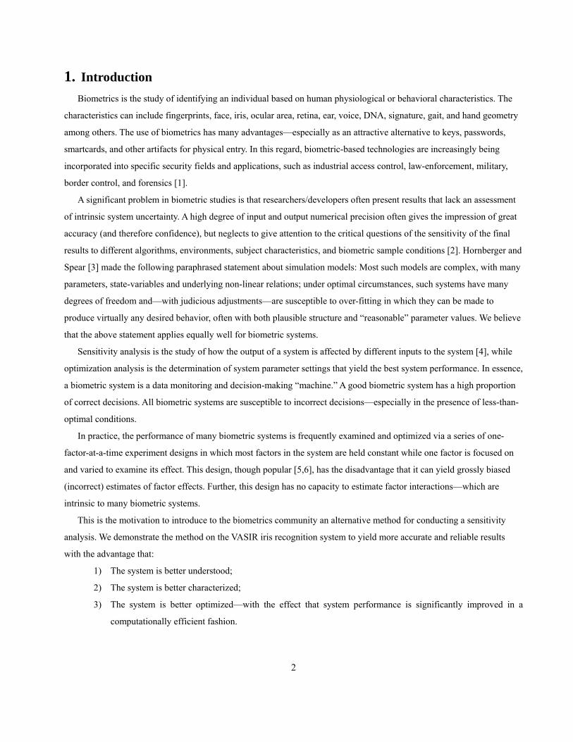
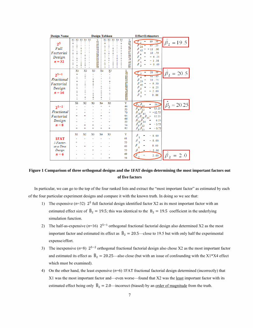
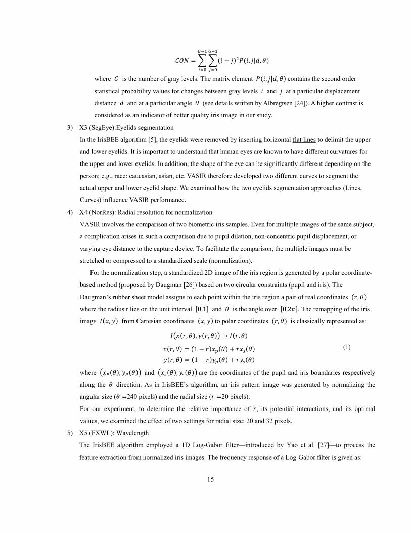

మቁబ
ఙ௪ଶ ቀ
మቁబ
௪௪ቀ
ൌ ሻݓሺܩ (2)
where ݓ represents the filterrsquos center frequency (wavelength) and σ gives the filter bandwidth We used
different wavelengths (18px 16px) to determine the relative importance of ݓ its interactions and its
optimal settings
6) X6 (FXMask) Wavelet magnitude
To encode coefficients (complex value) with the binary iris code [0 1] VASIR employed the phase
information with four quadrants proposed by Daugman [26] To determine each bit of the iris code for the
coefficient if the real part of the coefficient is negative the iris code is mapped to ldquo0rdquo otherwise it is mapped
to ldquo1rdquo If the imaginary part is negative the iris code is mapped to ldquo0rdquo otherwise it is mapped to ldquo1rdquo This is
to assure that unimportant bits would not be included when measuring the similarity between two biometric
templates [28] The paper written by Lee [7] suggested that VASIRrsquos approach based on the distance
(magnitude) of the coefficient from the origin is superior than the Hallingsworthrsquos fragile bit approach [28]
based on filter responses near the axes of the real or imaginary part We then examined what levels of
smalllarge magnitude values affect VASIR performance For this we varied the masking of significant bits
based on larger magnitudes (08 09)mdashthat is the effect of keeping 80 (vs 90 ) of the bits before
computing the similarity distance
7) X7 (SMAlg) Similarity metrics
Similarity metrics provide a quantitative measure for the degree that the two templates match A wide variety
of similarity metrics have been proposed in the iris-based biometrics community [293031] This section
compares and examines four similarity distance metrics (HD COR COS WED)
A Hamming Distance (HD)
The Hamming Distance counts the number of positions given two templates of the same size that
binary digits (0 and 1) are different [32] It can be used to decide whether two iris templates are of the
same person In VASIR a fractional HD was applied to its iris recognition systemmdashinitially proposed
by Daugman [29] and later re-implemented by Masek [5] A noise mask helps to exclude insignificant
bits (eg eyelashes eyelids reflections) of a template The fractional HD is given by
୧ୀଵሺT୧ oplusQ୧ሻ cap ሺTm୧ cap Qm୧ሻHDሺT Qሻ ൌ sum
N െ sum୩ୀଵሺTm୩ cup Qm୩ሻ
where target (T) and query (Q) are two bit-wise templates and Tm and Qm are the corresponding noise
masks N is the total bits of a template
B Normalized Cross-Correlation (COR)
COR is a measure of similarity between two templates for image processing The images are
normalized by subtracting the mean value and dividing by the standard deviation as follows
16
sum୧isinሼ୫ cap୫ ሽሺT୧ െ μTሻ sdot ሺQ୧ െ μQሻCORሺT Qሻ ൌ
ටsum ሺT െ μTሻଶ sdot sum ሺQ െ μQሻଶ୧isinሼ୫cap ୫ሽ ୧
୧ୀଵ ୧
QandTare the means of ߤ andμTwhere
C Cosine similarity (COS)
COS is a measure of similarity between two vectors by measuring the cosine of the angle the angular
separation is ሾെ1 1ሿ
sum୧isinሼ୫cap ୫ሽ T୧ sdot Q୧COSሺT Qሻ ൌ ටsum୧isinሼ୫ cap ୫ሽ T୧
ଶ sdot sum୧isinሼ୫cap ୫ሽ Q୧ଶ
D Weighted Euclidean Distance (WED)
WED can be used to determine similarity of an unknown sample set to a known one and is given as
WEDሺT Qሻ ൌ 1ொ൯ଶ ሺT୧ െ Q୧ሻ
ଶ
୧isinሼ୫cap ୫ሽ ൫ߪwhere ߪ is the standard deviation of the ith feature of the template Q
8) X8 (SMSh) Horizontal shifting
The starting point for normalizing the iris region of an iris image varies due to the subjectrsquos head tilt
movement and when the subject looks in a different directionmdashwe call this rotational inconsistency To
overcome this rotational inconsistency between two iris templates one template is two bit-wise shifted left or
right and the similarity score is selected from successive shifts [529] eg the smallest value is a successive
shift value for the Hamming Distance case
VASIR developed a new shifting method in which the template is shifted not only left and right (horizontal)
bit-wise but also upward and downward (vertical) the values for these horizontal and vertical direction shifts
are indicated by X and Y respectively We were interested in the effect of rotational inconsistency on VASIR
performance such inconsistency is linked to horizontal (as opposed to vertical) bitwise shifting and so we
varied such horizontal bitwise shifting (by two levels 5 and 10 bits) to determine the relative importance of a
number of shifted bits their potential interaction and their optimal settings
All remaining factors were fixed We should note that our conclusions about the chosen eight algorithmic factors may
be dependent on the settings of the remaining 30 (=38-8) algorithmic factors and the 33 robustness factors (see Appendix
A and Table 1 respectively)
It is a sobering reality that ldquonaturerdquo will propagate the effect of these remaining algorithmic and robustness factors
onto the performance of our VASIR system and onto our conclusions about the relative importance of these eight
factorsmdashregardless of whether we identify such factors or not For a good experiment design it is critically important to
pre-identify control or at least record the settings of these robustness factors during the entire course of the experiment
17
43 Responses ( )
Y refers to the response of interest for which we wish to evaluate the effect of the various factors In biometric systems
it is quite common to have multiple responses of interest and these responses are frequently identical to various
performance metrics
Our study had three responses that were based on similarity distance values for matching and non-matching scores 1)
the VR (Verification Rate) when the FAR (False Accept Rate) was 001 2) the VR when the FAR was 010 and 3) the
EER (Equal Error Rate)mdashthe detailed definition is described in the papers [733] Symbolically the three responses are
Y1 = VR|FAR = 01 (or TAR|FAR = 01)
Y2 = VR|FAR = 10 (or TAR|FAR = 10)
Y3 = EER
For a biometric system higher values of VR and smaller values of EER indicate superior system performance
Common alternatives for VR|FAR are FAR = 001 and FAR = 0001 We chose not to use these as our performance
metrics because they would not have been meaningful due to the relatively small number of different subjects (~70 to 100)
in the chosen MBGC dataset selected for our study
44 Max Affordable Number of Runs
Our computing platform consisted of a dual core CPU (333 GHz) and RAM (64 GB) with Windows Server 2008 as
the operating system The practical constraint under which our study was operating was that the total amount of CPU time
for the experiment in total would not exceed two weeks This maximum two-week time constraint was chosen to allow
for design re-execution due to possibility of ldquoreal worldrdquo negative events that many times do occur in large scientific
investigations eg crashes (hardwaresoftware) memory leaks debugging problems dataset problems design access
problems anomalous (unusual) looking results and data analysis problems In reality in light of all of the above
possibilities it did in fact take approximately six months to design collect data and carry out a sensitivity analysis for
the two-week run Hence even in a parallel computing environment this ideal two-week time constraint translated into an
upper limit of n=500 runs to examine the eight algorithmic factors
45 Choice of Design
Given the (k=8 factor n lt 500 run) constraint with six factors at two levels factor X2 at three levels and factor X7 at
four levels full factorial is an excellent design but too expensivemdashfar exceeding our n=500 limit ( ൌ 2 ൈ 3ଵ ൈ 4ଵ ൌ
768 for all possible combinations of all k=8 factors) On the other hand orthogonal fractional factorial design is excellent
with good main effects and interaction estimation properties and is highly efficient
The question then arises as to how to fractionate and what factors to fractionate on Since fractionating three- and
four-level factors is more difficult we choose to fractionate on the six factors at two levels this is referred to as a 2ଵ
design and is described in Box et al [12] (see p276) In combination with the other levels of the two factors the design
that we chose is a ሺ2ଵሻ ൈ ሺ3ଵሻ ൈ ሺ4ଵሻ orthogonal fractional factorial This design examines the eight algorithmic 18
factors with n=384 runmdashhalf the runs of a full factorial and well below our 500-run limit This design utilizes two levels
for each of the six algorithmic factors (X1 X3 X4 X5 X6 X8) three levels for X2 and four levels for X7 these two
levels will be coded as (-1 +1) three levels (-1 0 +1) and four levels (-2 -1 +1 +2)
The (k=8 factor n=384 run) ሺ2ଵሻ ൈ ሺ3ଵሻ ൈ ሺ4ଵሻ orthogonal design matrix that we employed is shown in Figure
3mdashnote that since some of the eight factors are more time-consuming to change than others the run order of the above
design was optimized to minimize execution time (a 4x speed-up was achieved)
Figure 3 A ሺሻ ൈ ሺሻ ൈ ሺሻ orthogonal fractional factorial design matrix for eight algorithmic factors in
VASIR (see the detailed design in Appendix B)
Note that this design matrix has 8 columns (factors) and 384 rows (runs) since the design is orthogonal each of six
two-level factors (X1 X3 X4 X5 X6 X8) has the same number (3842 = 192) of -1rsquos and +1rsquos X2 factor has three
settings (3843 = 128) of -1rsquos 0rsquos and +1rsquos while X7 has four settings (each occurring 3844 = 96) of -2rsquos -1rsquos +1rsquos and
+2rsquosmdashthis equality property is referred to as 1-dimensional balance
Due to orthogonality each and every one of the ൫ଶ൯ ൌ 15 pairs of the six factors at two levels has the same number
of (-1-1) (-1+1) (+1-1) and (+1+1) combinationsmdashnamely 324=8 this is referred to as 2-dimensional balance
For the ሺ2ଵሻ ൈ ሺ3ଵሻ ൈ ሺ4ଵሻ design we should obtain near-precise estimates of main effects and two-term
interactionsmdashrivaling the quality of a ሺ2ሻ ൈ ሺ3ଵሻ ൈ ሺ4ଵሻ full factorial designmdashbut with only half (384) the number of
runs
5 Data
51 Dataset
For the purpose of this sensitivity analysis study we evaluated the VASIR system performance using datasets
collected by MBGC (Multiple Biometric Grand Challenge) [34] These MBGC datasets include iris images of varying
illumination conditions low quality and off-angle or occluded images in both still and video imagery One of challenges
19
for the MBGC dataset is to recognize a person from the NIR and high definition video as the person walks through a
portal In this experiment we there use the NIR face-visible video dataset which we will call ldquodistant-videordquo the distant-
video samples were captured with a video camera by the Sarnoff IOM system in 2048x2048 resolutions with
facehairneck visible in the screen
For the MBGC distant-video dataset Table 4 shows the number of video sequences captured by IOM system
Table 4 Distant-video (face-visible) number of videos captured by IOM
Distant-Video MBGC
Total of videos 628
of used videos 204
A small number ( 50) of the subjects appeared in only one video sequencemdashand so these subjects were excluded
because we wanted to have replication over at least two videos at a different time Other subjects existed in multiple video
sequences some appeared in as many as ten sequences For parsimony if a subject happened to appear in three or more
video sequences we extracted for our study two such video sequencesmdasheach sequence representing a different session In
summary out of the 628 videos we thus used 204 videos involving 102 subjects
Figure 4 shows an example of distant-video within the MBGC dataset
Figure 4 Sub-images extracted from MBGC distant-video taken by IOM
20
Figure 4 (a) and (b) show the face-visible frame from a video and the sub-image (eye region) extracted from that
frame Distant-video data is normally considered to be a poor-quality image source since the video was taken with
moving subjects having motion blur poor contrast off-angle poor illumination and other deficiencies
52 Data Collection Procedure
This section describes the procedure of collecting data for our focus in this paper the left eye position and the face-
visible distant-video to distant video (VV) matching scenario For this VV matching scenario we used 204 videos (102
subjects) whereby each subject appeared in two different video sequences and each taken in different sessions
The VASIR system then proceeds as follows
1) VASIR automatically adjudges identifies and extracts all admissiblevisible left iris images (= 565 in this
case) out of these 204 video sequences (face-visible) based on criteria related to factor X1 (Eye region
detectionextraction with pupil position alignment)
2) VASIR then selectsmdashautomaticallymdashthe best 204 iris images based on quality score criteria associated with
factor X2 (Image quality metrics for quality assessment and the best image selection)
3) VASIR then takes the resulting 204 images and segments the iris region based on segmentation algorithms
that included factor X3 (eyelid segmentation algorithm)
4) The segmented iris regions are extracted using polar-coordinates and then normalized based on the resolution
related to factor X4 (Radial resolution)
5) VASIR extracts features from the normalized iris images based on the feature extraction algorithm associated
with factor X5 (wavelength)
6) Then VASIR encodes the extracted features and masks out noise based on factor X6 (masking with wavelet
magnitude)
7) The encoded results are then used for carrying out the pair-wise biometric templates matching based on factor
X7 (similarity metrics)
8) Finally to correct rotational inconsistencies between two biometric templates VASIR applies factor X8
(horizontal shifting)
The above VASIR procedure is executed for all n=384 runs of the k=8 factors as specified by the 2ଵ ൈ ሺ3ଵሻ ൈ ሺ4ଵሻ
experiment design For a given run we obtain a set of match scores and a set of non-match scores Based on the set of
match and non-match scores VASIR automatically produces similarity scores which in turn yields the three performance
responses (VR|FAR=01 VR|FAR=10 and EER) The sensitivity analysis was then initiated to determine the effect of the
eight algorithmic factors on the above three responses
6 Data Analysis
This section describes the details of the sensitivity analysis carried out on the k=8 algorithmic factors for the VASIR
system This analysis is carried out and presented for the fixed settings of the remaining algorithmic factors (see Appendix 21
A) and robustness factors (see Table 1) In particular the results presented in the remainder of this section are for the VV
matching scenario and the left eye position
The specific deliverables from the sensitivity analysis of the VASIR system are as follows
1) a ranked list of all eight algorithmic factorsmdashordered by relative importance
2) inclusion of the relevant interactions within that ranked list
3) estimates of the magnitude and the direction of factor effects and interactions
4) determination of the most important factor(s) and interaction(s)
5) specification of the optimal (local) settings for the eight factors
As we discussed in Section 22 to fulfill the goals in our study we demonstrate three especially important plots of the
ten graphical procedures 1) Main Effects plot 2) Interaction Effects Matrix plot and 3) Ordered Data plot
61 Main Effects Plot
The Main Effects plot is the most important graphical data analysis technique to identify the influential and
statistically significant factors affecting performance responses This plot provides the mean response for each setting of
each factor and highlights their difference to show the effect of changes on the response(s) due to that factor [15]
Figure 5 shows the Main Effects plot of VASIRrsquos k=8 factors on the VV Left case with the VR|FAR=01 performance
response
Figure 5 Main Effects plot with the VR|FAR=01 response for VV Leftmdashnote that the four coded settings (1234)
for X7 are equal to (-2-1+1+2) The importance of factors X2 X7 X3 X1 X8 and X4 in order
22
The horizontal axis illustrates the eight factors (X1 to X8) and the coded factor settings (eg ldquominus1rdquo ldquo0rdquo or ldquo+1rdquo) for
each factormdashthe four coded factor settings for X7 (1 2 3 and 4) are equivalently referred to as ldquo-2rdquo ldquo-1rdquo ldquo+1rdquo and
ldquo+2rdquo The vertical axis presents the mean response for each setting of each factor For each factor a line connects the
mean values for that factor The magnitude of the line is the factor effect longer lines indicate the factor has effects while
shorter lines indicate the factor has no effect The slope of the line indicates whether the factor has an increasing or
decreasing effect on VASIRrsquos responses
The number of runs (n) in the design was originally 384 = 2ଵ ൈ 3ଵ ൈ 4ଵ Some of the runs are ignored if the
response value does not exist (due to a small number of subjects) for the relevant run therefore n may be less than 384
For example the legend box of the Figure 5 plot has n=383 because one value out of the 384 doesnrsquot exist for this
VR|FAR=01 response
On the inside of the plot above the horizontal axis the top number gives the percentage from a one-way ANOVA f-test
two asterisks () signifies that a factor effect is statistically significant at the 1 level ( 099) and one asterisk ()
signifies significance at the 5 level ( 095 099) The second number is the estimated factor effect in raw response
units In case of factors with two-level settings (coded as minus and + and with corresponding mean values ݕത and ݕതା) the
effect is uniquely defined as ݕതା െ തݕ For three-level settings (minus 0 and + and with corresponding mean values ݕത തݕ
and ݕതା) we define the factor effect as the largest in magnitude out of given three differences ݕതା െ തݕ തା െݕ ത andݕ
ത െݕ തݕ For four-levels we also define the factor effect as the largest out of ൫ସଶ൯=6 possible differences The bottom
number is the estimated percentage change (relativeeffect ൌ 100 ൈ effectglobalmean) Note that since the design is
orthogonal such effect estimates are identically the least squares estimates that would result from a multi-linear
regression
For the response VR|FAR=01 of the VV Left eye case the important factors influencing VASIRrsquos performance are
ordered by
X2 (IQMetr) Image quality metrics (effect = 041) followed closely by
X7 (SMAlg) Similarity metrics (effect = 038)
X3 (SegEye) Eyelids segmentation (effect = 026)
X1 (EyeAlg) Eye position alignment (effect = 020)
X8 (SMSh) Horizontal shifting (effect = 017) and then
X4 (NorRes) Radial resolution for normalization (effect = 011)
X6 (FXMask) Wavelet magnitude (effect =006) and
X5 (FXWLBW) Wavelength (effect = 003)
Six factors (X2 X7 X3 X1 X8 and X4) are statistically significant ( or ) and are highlighted in red two factors
(X5 and X6) are not statistically significant
The Main Effects plot is also useful for determining optimal settings on the averagemdashie based on actual settings
utilized in the experiment design From Figure 5 those settings for each factor which yield a large value (closer to 10) of
23
VR would be the preferred optimal setting The optimal settings are (+1minus1 +1 +1 bull bull +2 +1) where ldquobullrdquo indicates both
settings are equivalent or the mean difference is not statistically significant
From the Main Effects plots a summary of the factor effects and optimal settings for all three responses is given in
Table 5
Table 5 VASIRrsquos most important (IMP) factors and optimal settings with three responses for VV Leftmdashfrom Main
Effects plots
Responses 1st Most
IMP
2nd Most
IMP
Least
IMP
Optimal Setting
X1 X2 X3 X4 X5 X6 X7 X8
VR|FAR=01 X2 X7 X5 X6 +1
(ON)
minus1
(SOB)
+1
(Curves)
+1
(32)
bull (minus1)
(18)
bull (+1)
(9)
+2
(WED)
+1
(5)
VR|FAR=10 X2 X3 X5 X6 +1
(ON)
minus1
(SOB)
+1
(Curves)
+1
(32)
bull (minus1)
(18)
bull (minus1)
(8)
minus2
(HD)
+1
(5)
EER X2 X3 X5 X6 +1
(ON)
minus1
(SOB)
+1
(Curves)
+1
(32)
bull (minus1)
(18)
bull (minus1)
(8)
minus2
(HD)
+1
(5)
represent statistical significance at the 1 levels respectively
bull represents that the mean difference between settings is not statistically significant
For all three responses the most important factor out of these eight algorithmic factors in VASIR is X2 (IQMetr) and
the second important factor X3 (SegEye) and X7 (SMAlg) The statistically significant factors having an influence on the
VASIR system are (X2 X7 X3 X1 X8 and X4) in order from most to least important The least important factors are
X5 (FXWL) and X6 (FXMask) for all responses
62 Ordered Data Plot
The Ordered Data plot yields the settings that correspond to each response value The plot is generated by ordering all
n responsesmdashworst to bestmdashand carrying along the corresponding settings for the k=8 factors If a factor has one setting
for the best and near-best response values and the opposite setting for the worst and near-worst response values then that
factor is usually a relatively important factor [10] Ordered Data plots can reconfirm the results from main effects
Figure 6 illustrates the Ordered Data plot for the VR|FAR=01 response for the VV Left case In our sensitivity
analysis we used a total of 384 runs from the eight algorithmic factors and so the plot potentially contains a maximum of
384 data points for example the Ordered Data plot in Figure 6 has only 383 runs for the VR|FAR=01 response
Presenting all data points and their settings make the plot too crowded and difficult to interpret the data properly So
we illustrated only the 60 most important extreme pointsmdashthe best and near-best response values (30 points) on the right-
side and the worst and near-worst response values (30 points) on the left-side the inserted blue vertical line distinguishes
between the best-side and worst-side points
24
The upper left corner box of the plot shows the number of factors (k=8) and the number of data points (60) followed
by the total number of runs (383) that have the corresponding VR|FAR=01 response The horizontal axis shows the eight
factor labels and their settings for each of the 60 runs ordered from the smallest to the largest response values The
vertical axis is the value of the VR|FAR=01 response
Figure 6 Ordered Data plot with VR|FAR=01 response for VV Left We illustrated only the 60 most important
extreme pointsmdash30 (best) + 30 (worst)
The Ordered Data plot not only provides the best settings but also reaffirms important factors On the average if a
factor has no effect then there should be a near even split of 15 +1rsquos and 15 -1rsquos the more the divergence from 1515 the
greater the significance of the factor For 30 trials it is statistically significant whenever the count is 20 or 10 For
instance we may pose the question as to whether factor X1 (EyeAlg) is important Out of the 30 best VR|FAR=01
responses 29 of them came with X1=+1 For the 30 worst responses 22 came from X1=-1 Thus X1 (EyeAlg) is an
important factor
Table 6 summarizes the counting levels from the plot in Figure 6 Highlighted in orange are the counts of two levels
20 for the best response and 10 for the worst responsemdashnote that since factor X7 has four levels the criteria for
this count is 12 and 2 respectively and for the three levels of factor X2 the criteria is 15 and 5 Based on
the above table we thus conclude that the important factors for VR|FAR=01 are as follows X1 (EyeAlg) X2 (IQMetr)
X3 (SegEye) X7 (SMAlg) and X8 (SMSh)mdashwhere both worst and best responses were highlighted in orange From
Figure 6 the best settings for the VR|FAR=01 response are (+1minus1 +1 +1 minus1 minus1 +2 +1)mdashwhich is exactly the same as
the results from the Main Effects plot in Figure 5
25
Table 6 Summary of counting levels for the VR|FAR=01 worstbest response
Factor Worst response Best response
-2 -1 0 +1 +2 -2 -1 0 +1 +2
X1 (EyeAlg) 22 8 1 29
X2 (IQMetr) 5 19 6 27 2 1
X3 (SegEye) 20 10 9 21
X4 (NorRes) 19 11 8 22
X5 (FXWL) 9 21 15 15
X6 (FXMask) 21 9 14 16
X7 (SMAlg) 1 10 8 1 11 4 2 13
X8 (SMSh) 21 9 7 23
Table 7 shows the summary of important factors and the best settings ndashyielded from the Ordered Data plotmdashfor the
VV Left case
Table 7 VASIRrsquos relative important factors and the best settings with three responses for VV Leftmdashfrom Ordered
Data plots
Responses Important Factors Best Setting
X1 X2 X3 X4 X5 X6 X7 X8
VR|FAR=01 X1 X2 X3 X7 X8 +1
(ON)
minus1
(SOB)
+1
(Curves)
+1
(32)
minus1
(18)
minus1
(8)
+2
(WED)
+1
(5)
VR|FAR=10 X1 X2 X3 X8 +1
(ON)
minus1
(SOB)
+1
(Curves)
minus1
(24)
+1
(16)
minus1
(8)
minus2
(HD)
+1
(5)
EER X2 X7 X8 +1
(ON)
minus1
(SOB)
+1
(Curves)
+1
(32)
minus1
(18)
minus1
(8)
minus2
(HD)
+1
(5)
From the analysis of all responses for this VV Left case in Ordered Data plots factors X1 (EyeAlg) X2
(IQMetr) X3 (EyeSeg) X7 (SMAlg) and X8 (SMSh) are the important factors and the best settings are (+1minus1 +1
+1 minus1 minus1 minus2 +1)mdashwhich is relatively similar to the results derived from the Main Effects plots
63 Interaction Effects Matrix
Knowledge of the main effects is an incomplete description of the influence of factors because interactions exist
among factorsmdashcomplex systems such as biometrics are frequently more complicated than simple (linearadditive)
models When a factor effect changes by depending on the setting of another factor the two factors are said to interact
and those interaction effects must be considered For factors A and B with two levels (+1 and -1) the interaction effect is
estimated by calculating the factor A effect (when factor B is at the + level) calculating the factor A effect (when factor B
is at the ndash level) and then differencing the two factor A effects If there is no interaction between the two factors A and 26
B then the factor A effect will be the same for both and hence the difference will be 0 We now address the problem as to
whether two-term interaction effects exist in the VASIR system and determine whether those interaction effects are
important VASIR has ൫ଶ൯ ൌ 28 such two-term interactions among the eight algorithmic factors
There are two methods to represent the interaction effects between the two factors
1) interaction effects with two-levels and
2) interaction effects with three or more levels
For the first method where the two factors have only two levels the representation becomes simpler In such cases
the factor cross products serve as a reasonable surrogate for the interactions In particular if factor X1 takes on the coded
values -1 and +1 and if factor X2 takes on the coded values -1 and +1 then the cross product X1X2 also takes on the
coded values -1 and +1
ሺെ1ሻ ൈ ሺെ1ሻ ൌ 1
ሺെ1ሻ ൈ ሺ1ሻ ൌ െ1
ሺ1ሻ ൈ ሺെ1ሻ ൌ െ1
ሺ1ሻ ൈ ሺ1ሻ ൌ 1
The advantage of this method is that the cross product X1X2 (and for that matter any cross product) becomes just
another -1 and +1 factor in the orthogonal system and so the interaction effects may be directly estimated and compared
with one another and with the algorithmic factors On the other hand if the two factors have three or more levels then the
representation of such interactions is more complicated and the cross product representation is of little help For our case
the eight algorithmic factors have different levels six factors have two levels the factor X2 has three levels and X7 four
levels
With this in mind we make use of the Interaction Effects Matrix plot (see Figure 7 below) which is a multi-plot per
page display of the original main effects and all of the two-term interactions In practice for an experiment with k factors
the total number of possible two-term interactions is
ሻ െ 1ሺൌ
൬2൰ ൌ2 ሺ െ 2ሻ 2
In our experiment we have 28 two-term interactions from a (2ଵ ൈ 3ଵ ൈ 4ଵ) experiment ( ൌ 8) for each response
Figure 7 presents the interaction effects matrixmdashit consists of 64 plots (8 Main Effects plots + 2 ൈ 28 Interaction Effects
plots)mdashtwo plots for each two-term interaction
27
Figure 7 Interaction Effects Matrix plot with the VR|FAR=01 response for VV Left The blue circles indicate
significant factors and the red circles indicate two-term interactions where effects appear significant
The plots on the diagonal are identical to those seen on the Main Effects plot the horizontal axis is the factor levels
and the vertical axis is the mean response at each of those levels the index in the upper left corner identifies factors (eg
X1) and the number following the index is the (least squares) estimated effect due to that factor (eg X1 (+1) effect
βଵ ൌ 02)
The plots off-diagonal are the two-term interaction plots the index in the upper left corner of each plot identifies the
two-term interaction (eg X1X2 X1X3) For the X1X2 interaction (X1 with two levels and X2 with three levels) the
horizontal axis is the two levels of X1 and the vertical axis is the mean response at each of those two levels it is
computed three timesmdashonce for each level of X2mdashthus yielding six (=2x3) points and three traces From each of the
three traces we can compute an X1 effectmdashthe steeper the trace the larger the X1 effect When the three traces are
parallel then the resulting three estimates of the X1 effect are identicalmdashand so the factor X1 effect is not dependent on
the level of X2 (no interaction) When the three traces are not parallel then the X1 effect depends on the setting of X2
(interaction)
In summary the Interaction Effects plots are interpreted as follows
1) If the lines within the plot are parallel then this implies no interaction
2) If the lines within the plot are not parallel this implies an interactionmdashthe more divergent the stronger the
interaction
If there is no interaction among factors we can conclude that the system response is driven primarily by main effects
Otherwise the interactions can lead to unexpected effects on the responses
28
For the VR|FAR=01 response in the VV Left case Figure 7 shows the relative importance of factors X2 X7 X3 X1
X8 and X4 in ordermdashsee the blue circles on the diagonal For the most important factor X2 it is seen that there exists an
interaction effect between X1 (EyeAlg) and X2 (IQMetr)mdashsee the non-parallel lines in the X1X2 and X2X1 Similar
cases are seen between X1 (EyeAlg) and X3 (SegEye) and between X6 (FXMask) and X7 (SMsh)mdashsee the red circles
on the off-diagonal
The Interaction Effects Matrix plot for VR|FAR=01 response shows that almost all of the 2 ൈ 28 plots have near-
parallel traces and hence do not interactmdashonly three two-term interactions exist with non-parallel lines out of 28
1) X1 and X2 (EyeAlg and IQMetr)
2) X1 and X3 (EyeAlg and EyeSeg)
3) X6 and X7 (FXMask and SMAlg)
Thus only a few of the eight algorithmic factors are interacting with one another to affect the VR|FAR=01 VASIR
matching performance response
Table 8 summarizes the results from all three responses interaction effects analysis one per response
Table 8 Summary of VASIRrsquos interaction effects with three responses for VV Left
Response Interaction Effects
VR|FAR=01 X1X2
(EyeAlgbullIQMetr) X1X3
(EyeAlgbullSegEye) X6X7
(FXMaskbullSMAlg)
VR|FAR=10 X1X2
(EyeAlgbullIQMetr) X1X7
(EyeAlgbullSMAlg)
EER X1X2
(EyeAlgbullIQMetr) X1X7
(EyeAlgbullSMAlg)
For this VV Left eye case the X1X2 (EyeAlgbullIQMetr) interaction occurred for all three responses and the X1X7
(EyeAlgbullSMAlg) interaction for only the VR|FAR=10 and EER responses
The most important interaction effects are between factor X1 (Eye position alignment) and X2 (Image quality metrics)
for the VASIR VV Left case The interaction effects with factor X1 (EyeAlg) appeared the most frequently followed by
X2 (IQMetr) and X7 (SMAlg) The results show that X3 (SegEye) X4 (NorRes) X5 (FXWLBW) X6 (FXMask) and X8
(SMsh) barely have any interaction in the VASIR system
The results indicated that almost all of the 28 interaction plots have parallel tracesmdashonly 2 or 3 interaction effects out
of 28 Thus we conclude that the VASIR system is a near-linear systemmdashdriven by main effects with virtually little effect
from interactions Such near-linearity suggests that algorithmic changes to optimize a particular factor of interest are
unlikely to influence the effects of other algorithmic factors in the VASIR system (quasi-independence)mdashnote that this
conclusion may change depending on other remaining algorithmic factors and robustness conditions
29
64 ROC Curve
The ROC (Receiver Operating Characteristic) curve is a plot of FAR (False Accept Rate) against VR (Verification
Rate) which presents the tradeoff between the estimates of the verification rate and false accept rate In an ideal system
the FAR should be low and the VR should be high
Figure 8 Comparisons of the VASIRrsquos best and worst settings for VV Left
We now address the question as to how good the optimal settings are as compared to other possible settings for the
VASIR system Figure 8 illustrates the comparison between the best setting (+1minus1 +1 +1 minus1 minus1 minus2 +1) and the worst
setting (minus1 0 minus1 minus1 +1 +1 +1 minus1) (as obtained from the Main Effects plot analysis) by plotting the corresponding
ROC curves
Based on the ROC curve when the settings were changed from worst (orange line) to best (green line) VR at
FAR=01 in VASIRrsquos performance increased approximately 128 EER decreased approximately 92
These results show that factor settings do make a difference This also demonstrates the efficiency and the power of
the orthogonal experiment design approach for setting characterizing and optimizing multiple factors simultaneously
7 Results
This section is a summary of the results for the factor effects most important to least important factors optimal
settings and performance improvement
30
For this VV Left case the ranked list of factors is (X2 X7 X3 X1 X8 X4 X6 X5) of which six factors X2 through
X4 are statistically significant factors X6 and X5 are not statistically significant Factor X2 (IQMetr) is image quality
metrics and factor X7 (SMAlg) is similarity metricsmdashthese are the two most important algorithmic factors affecting
VASIR performancemdashthis is robustly true over all three responses Factors X5 (FXWL wavelength) and X6 (FXMask
wavelet magnitude) are universally the least important factors for the three responses The overall improvement in the
VR|FAR=01 change from the worst to best settings of the eight factors was significantmdashVR at FAR=01 in VASIRrsquos
performance increased 128 and EER decreased 92 We demonstrated that the experiment design we employed was
very efficient and effective in determining which factors are important interaction effects and optimal settings
The eight algorithmic factors and our detailed findings that are new and unexpected are as follows
1) X2 (IQMetr) Image quality metrics
Out of the eight examined factors factor X2 (IQMetr) was the most important factor affecting VASIR
performance for all three responses Measuring image quality and then selecting the best quality image using
quality metrics had a strong factor effect (eg effect=041 at VR|FAR=01) on VASIRrsquos performance
responses and the effect was statistically significant The three settings of IQMetr consist of SOB (Sobel)
CON (Contrast) and LoG (Laplacian of Gaussian) SOB was introduced as a tool for face image quality
evaluation by Beveridge et al [19] CON was first introduced for general quality assessment by Albregtsen
[24] LoG was specifically used for the iris image quality assessment by Wan et al [35] For this VV Left
case we found that the SOB setting led to the best matching performance and was statistically different
(better) than the other two IQMetr settings CON (second best) and LoG (worst) The discrepancy between
SOB and LoG is a bit surprising since both the SOB and LoG approaches measure the focus based on edge-
based spatial domain metrics while the CON approach measures the contrast based on a GLCM (Gray Level
Co-occurrence Matrix) Hence SOB gave the best results in our iris verification experiments Unexpectedly
contrast (CON) was (slightly) better than the LoG operator We also found that X2 (IQMetr) had significant
interactions with factor X1 (EyeAlg Eye Position Alignment) As expected the best settings for the (EyeAlg
IQMetr) combination was (ON SOB) and the worst setting was (OFF LoG)
2) X7 (SMAlg) Similarity metrics
The second most important factor affecting VASIR performance was SMAlg (Similarity metric) The
similarity metrics are important (effect=038 at VR|FAR=01) and statistically significant The motivation for
this factor is to identify one metric as best for VASIR performance
The four settings for SMAlg are HD (Hamming Distance) COR (Correlation) COS (Cosine) and WED
(Weighted Euclidean Distance) Interestingly for the VR|FAR=01 response WED had slightly better
matching results than the other three metrics On the other hand for both VR|FAR=10 and EER responses
HD led to much better matching performance than the other metrics In summary HD had the best matching
31
results followed by COR WED and COS SMAlg had minor interactions with factor X1 (EyeAlg Eye
position alignment) and factor X6 (FXWL Wavelet magnitude)
3) X3 (SegEye)Eyelids segmentation
We found that the eyelids segmentation is an important factor (effect=026 at VR|FAR=01) and statistically
significant for all three responses This factor examines the effect of different algorithms for eyelids
segmentation The two settings for SegEye are ldquoLinesrdquo and ldquoCurvesrdquo For all three responses the use of two
different curves for segmenting the upper and lower eyelids led to a better matching performance than the use
of horizontal flat linesmdashthis was expected This conclusion reaffirmed that VASIRrsquos eyelid segmentation
approach [7] has a significant improvement over IrisBEErsquos approach [5] The presence of parallel lines in the
Interaction Effect Matrix for factor SegEye with the other seven factors (apart from minor interaction with
factor X1 [EyeAlg Eye position alignment]) indicates no interaction effect hence SegEye is primarily driven
by the main effect
4) X1 (EyeAlg) Eye position alignment
Eye position alignment is also an important factor (effect=020 at VR|FAR=01) and statistically significant
for all three responses This factor addresses the difficulty in iris recognition from rotational differences
between the target and query iris templates caused by tiltedrotated head with various movements The two
settings for EyeAlg are ON (correcting the inconsistency using an eye position alignment algorithm) and
OFF (not correcting the inconsistency) VASIR had a better matching performance when the system used the
ON setting to correct the rotational inconsistency between the two templates EyeAlg had significant
interactions with factor X2 (IQMetr Image quality metrics) X3 (EyeSeg Eyelids segmentation) and X7
(SMAlg Similarity metrics) As expected the best setting for the (EyeAlg IQMetr EyeSeg SMAlg)
combination was (ON SOB Curves HD) and the worst setting was (OFF LoG Lines COS)
5) X8 (SMSh) Horizontal bit shifting for the HD_XorY approach
Horizontal bit shifting is important (effect=017 at VR|FAR=01) and statistically significant The motivation
of this factor is to correct rotational inconsistencies after normalizing the target and query template Masek [5]
used 3 bits shifting for left and right for the LEI [36] dataset and 8 bits for the CASIA [37] dataset IrisBEE
[17] used 10 bits shifting for the ICE2005 [17] dataset For VASIR we examined the use of 5 and 10 bits
shifting for the MBGC video dataset The two settings for SMSh are therefore 5 and 10 We found that 5 bits
shifting had better matching performance than 10 bits shifting across all three responses Note that factor
SMSh had no interaction with other factors hence this factor could be optimized independently without
adversely affecting other factors
6) X4 (NorRes) Radial resolution for normalization
The last statistically significant factor is radial resolution (effect=011 at VR|FAR=01) This factor addresses
the question as to whether template size affects VASIR performance the two settings for NorRes are 20px
32
and 32px We found that the larger radius resolution (32px) had a better matching performance than the
smaller resolution (20px) across all three responses NorRes does not interact with other factors
7) X6 (FXMask) Wavelet magnitude
Wavelet magnitude is unimportant (effect=006 at VR|FAR=01) and statistically insignificant This factor
examines the effect of declaring different levels () of important bits in the iris template The two settings of
FXMask are 08 (80 ) and 09 (90 ) For the VV Left case the 80 setting is slightly (but not
significantly) better than the setting 90 for all three VASIRrsquos responses Note that FXMask has a minor
interaction with X7 (SMAlg Similarity metrics)
8) X5 (FXWL) Wavelength
The least important factor in our study is wavelength (effect=003 at VR|FAR=01)mdashit is statistically
insignificant This factor examines the effect of varying the center frequency of the Log-Gabor filter (for
feature extraction) on VASIR performance The two settings of FXWL are 16px and 18px (the IrisBEE
default) Our study found that 18px was slightly (but not significantly) better than 16pxmdashthe difference is
negligible Masek [5] found that 18px was also optimal for the CASIA datasetmdashalthough the author stated
that the optimal value can be attributed to the different imaging conditions of each dataset On the other hand
our orthogonal experiments showed that difference in effect between16px and 18px for MBGC video is
insignificant In comparing our results to Masekrsquos results two principal differences emerge 1) the Masek
experiment varied a few (one or two) factors the VASIR experiment varied k=8 factors 2) the VASIR
experiment design allowed for the existence of interactions Both of these reasons support the contention that
the VASIR conclusions are more global and robust FXWL had no interaction effect with any other factors
8 Conclusions
We introduced to the biometrics community a structured methodology for sensitivity analysis to foster an
understanding of the key factors (parameters) in biometric systems
This Sensitivity Analysis methodology consists of two components
1) Experiment design in which we utilize efficient orthogonal fractional factorial designs to estimate not only the k
main effects but also the ൫୩ଶ൯ two-term interactions of a biometric system
2) Graphical data analysis in which we utilize three procedures Main Effects plot Ordered Data plot and
Interaction Effects matrix to determine important factors two-term interactions and optimal (local) settings
To demonstrate the utility of this methodology using the MBGC distant-video dataset we chose a (k=8 factor n=384
run) ሺ2ଵሻ ൈ ሺ3ଵሻ ൈ ሺ4ଵሻ orthogonal fractional factorial experiment design for our VASIR systemmdashinvestigating eight
algorithmic factors (X1 to X8) to determine the most important their optimal settings and the relative importance of the
28 two-term interactions
For this Video to Video (VV) Left eye case (the focus of this paper) our experiments showed that the three most
important (see bold below) out of these eight algorithmic factors that we studied in VASIR were X2 (IQMetr Image 33
quality metrics) with factors X3 (SegEye Eyelids segmentation) and X7 (SMAlg Similarity metrics) being next in
importance The least important factors were X5 (FXWL FX wavelength) and X6 (FXMask FX masking with
magnitude) We found that the optimal settings were (+1 minus1 +1 +1 minus1 +1 minus2 +1) with details as follows
- X1 (EyeAlg) Eye position alignment (+1 ON)
- X2 (IQMetr) Image quality metrics (minus1 Sobel operator [SOB])
- X3 (SegEye) Eyelids segmentation (+1 Curves)
- X4 (NorRes) Radial resolution for normalization (+1 32)
- X5 (FXWL) FX wavelength (minus1 18)
- X6 (FXMask) FX masking with magnitude (+1 09)
- X7 (SMAlg) Similarity metrics (minus2 Hamming distance [HD])
- X8 (SMsh) Horizontal shifting number (+1 5)
In order of decreasing importance the statistically significant factors that had an influence on VASIR performance
were the six factors (X2 X7 X3 X1 X8 and X4) On the other hand factors X5 and X6 were found to have barely any
effect on VASIRrsquos overall performance
We found that some two-term interactions did in fact existmdashthey involved factors X1 (EyeAlg) (primarily) X2
(IQMetr) and X7 (SMAlg)mdashin particular the X1X2 and X1X7 interactions were found to be important On the other
hand for our VV Left eye case we found that most of the interactions had minor effect on VASIR performancemdashhence
the effect on performance of VASIRrsquos algorithmic component was mostly additive and independent It is noteworthy that
when the VASIR settings were changed from worst to best VASIRrsquos verification rate at FAR=01 increased significantly
(128 ) and EER decreased significantly (92 )
In summary the choice of the image quality metric for selecting the best quality image in video had the strongest
effect on VASIR performance followed by the choice of similarity metric Our data analysis also reaffirmed that eyelid
segmentation was important and that VASIRrsquos approach (Curves) had a significant improvement over IrisBEErsquos approach
(Lines) Further VASIRrsquos two factors for correcting rotational difference due to head tilt or subject movement (eye
position alignment Horizontal shifting) were both important It is of interest to note that comparing across studies we
found that optimal value of bit shifting for correcting inconsistency depended on the dataset (or the different imaging
conditions of the dataset) Finally we found that the larger radius size of the iris template had a better matching
performance than the smaller size Given eight algorithmic factors we found that VASIR is a near-linear system thus
optimization of a particular factor is unlikely to influence the effects of the other algorithmic factors We believe that the
sensitivity analysis methodology demonstrated herein can be applied to other biometric systems
Based on our study opportunities for future research would include as follows 1) carrying out a follow-up experiment
to ascertain the robustness of our conclusions over other scenarios (eye position (leftright) matching scenarios (VV
Video to Video VS Video to Still and SS Still to Still) 2) replacement of the two unimportant factors with other VASIR
key algorithm factors and 3) applying the same sensitivity analysis methodology to simultaneously examine a
considerably larger (eg k=20 factor) set of VASIR algorithmic factors
34
Disclaimer
The identification of any commercial product or trade name does not imply endorsement or recommendation by the
National Institute of Standards and Technology (NIST)
References
[1] A K Jain P J Flynn and A A Ross ldquoIntroduction to Biometricsrdquo Handbook of Biometrics Springer 2008
[2] G Stirling Andrew ldquoOn Science and Precaution in the Management of Technological Riskrdquo European Science and
Technology Observatory 2002
[3] G M Hornberger and S RC ldquoAn approach to the preliminary analysis of environmental systemsrdquo Journal of
Environmental Management vol 12 pp 7ndash18 1981
[4] A Saltelli ldquoSensitivity analysis for importance assessmentrdquo Risk Analysis vol 22 no 3 pp 579ndash590 2002
[5] L Masek and P Kovesi ldquoMATLAB Source Code for a Biometric Identification System Based on Iris Patternsrdquo
School of Computer Science and Software Engineering University of Western Australia 2003
[6] K Messer J Kittler M Sadeghi M Hamouz A Kostyn S Marcel S Bengio F Cardinaux C Sanderson N
Poh and others ldquoPerformance Characterization of Face Recognition Algorithms and Their Sensitivity to Severe
Illumination Changesrdquo Biometric Authentication pp 8ndash19 2004
[7] Y Lee ldquoVASIR Video-based Automatic System for Iris Recognitionrdquo Dissertations School of Computer Science
and Engineering in Chung-Ang University South Korea 2011
[8] J J Filliben S Cetinkunt W L Yu and A Donmez ldquoExploratory Data Analysis Techniques as Applied to a High-
Precision Turning Machinerdquo Elsevier Science Publishers BV p 199 1993
[9] J J Filliben ldquoExperiment Design for Scientists and Engineersrdquo Short Course National Institute of Standards and
Technology 2002
[10] National Institute of Standards and Technology ldquoEngineering Statistics HandBook (559 An EDA approach to
experimental design)rdquo National Institute of Standards and Technology 2003 Available
httpwwwitlnistgovdiv898handbookprisection5pri59htm [Accessed 09-Mar-2011]
[11] J P Kleijnen ldquoDesign and analysis of Monte Carlo experimentsrdquo Handbook of Computational Statistics vol 1
2004
[12] G E P Box W G Hunter and J S Hunter ldquoStatistics for experimenters an introduction to design and model
buildingrdquo New York Singapore John Wiley 1978
[13] G EP Box J S Hunter and W G Hunter Statistics for Experimenters Design Innovation and Discovery 2nd
Edition Wiley 2005
[14] J J Filliben and A Hecket ldquoDataplot Homepagerdquo Available httpwwwitlnistgovdiv898softwaredataplot
[Accessed 11-Jul-2011]
35
[15] K L Mills J J Filliben C Dong Yeon S Edward and G Daniel ldquoChapter 4 Sensitivity Analysis of MesoNetrdquo
Study of Proposed Internet Congestion-Control Mechanisms 2010 Available
httpwwwnistgovitlantdCongestion_Control_Studycfm [Accessed 09-Mar-2011]
[16] J J Filliben ldquoDATAPLOTmdashAn Interactive High-level Language for Graphics Non-linear Fitting Data analysis
and Mathematicsrdquo ACM SIGGRAPH Computer Graphics vol 15 no 3 1981
[17] P J Phillips K W Bowyer P J Flynn X Liu and W T Scruggs ldquoThe iris challenge evaluation 2005rdquo The 2nd
IEEE International Conference on Biometrics Theory Applications and Systems (BTAS 2008) pp 1ndash8 2008
[18] Y Lee P J Phillips and R Micheals ldquoAn automated video-based system for iris recognitionrdquo Advances in
Biometrics pp 1160ndash1169 2009
[19] J R Beveridge G H Givens P J Phillips B A Draper and Y M Lui ldquoFocus on quality predicting FRVT 2006
performancerdquo in 8th IEEE International Conference on Automatic Face amp Gesture Recognition pp 1ndash8 2009
[20] R C Gonzalez and R E Woods Digital Image Processing 2nd ed Prentice Hall 2002
[21] N Kanopoulos N Vasanthavada and R L BAKER ldquoDesign of an Image Edge Detection Filter Using the Sobelrdquo
IEEE JOURNAL OF SOLID-STATE CIRCUITS vol 23 no 2 1988
[22] R Wang ldquoLecture Notes Computer Image Processing and Analysisrdquo 2011 Available
httpfourierenghmcedue161lecturesgradient [Accessed 21-Oct-2011]
[23] S R Gunn ldquoOn the discrete representation of the Laplacian of Gaussianrdquo The Journal of the Pattern Recognition
vol 32 pp 1463ndash1472 1999
[24] F Albregtsen ldquoStatistical Texture Measures Computed from Gray Level Coocurrence Matricesrdquo Image Processing
Laboratory Department of Informatics University of Oslo 1995
[25] M Hall-Beyer ldquoGLCM Texture Tutorialrdquo Available httpwwwfpucalgarycamhallbeytutorialhtm [Accessed
02-Jul-2011]
[26] J G Daugman ldquoHigh confidence visual recognition of persons by a test of statistical independencerdquo IEEE
Transactions on Pattern Analysis and Machine Intelligence vol 15 no 11 pp 1148ndash1161 2002
[27] P Yao J Li X Ye Z Zhuang and B Li ldquoIris recognition algorithm using modified log-gabor filtersrdquo Pattern
Recognition vol 4 pp 461ndash464 2006
[28] K P Hollingsworth K W Bowyer and P J Flynn ldquoThe best bits in an iris coderdquo IEEE Transactions on Pattern
Analysis and Machine Intelligence pp 964ndash973 2008
[29] J Daugman ldquoHow Iris Recognition Worksrdquo IEEE Transaction on Circuits System and Video Technology vol 14
no 1 pp 21ndash30 Jan 2004
[30] R P Wildes ldquoIris recognition an emerging biometric technologyrdquo Proceedings of the IEEE vol 85 no 9 pp
1348ndash1363 2002
[31] S Lim K Lee O Byeon and T Kim ldquoEfficient iris recognition through improvement of feature vector and
classifierrdquo ETRI journal vol 23 no 2 pp 61ndash70 2001
36
[32] Hamming RW ldquoError Detecting and Error Correcting Codesrdquo The Bell System Technical Journal vol XXIX p 2
1950
[33] P Grother R Micheals and P J Phillips ldquoFace Recognition Vendor Test 2002 Performance Metricsrdquo Fourth
International Conference on Audio-Visual Based Person Authentication 2003
[34] P J Phillips P J Flynn J R Beveridge K W Bowyer W T Scruggs A OrsquoToole and et al ldquoOverview of the
Multiple Biometrics Grand Challengerdquo The third IAPRIEEE International Conference of Biometrics (ICB2009)
pp705-714 2009
[35] J Wan X He and P Shi ldquoAn Iris Image Quality Assessment Method Based on Laplacian of Gaussian Operationrdquo
in Proc IAPR IAPR Conf Machine Vision Applications pp 248ndash251 2007
[36] C Barry and N Ritter ldquoDatabase of 120 Greyscale Eye Imagesrdquo Lions Eye Institute Perth Western Australia
[37] Center for Biometrics and Security Research (CBSR) ldquoCASIA Iris Image Databaserdquo Service Note on CASIA Iris
Image Databases Available httpwwwcbsriaaccnIrisDatabasehtm [Accessed 31-Aug-2011]
37
Appendix A The chosen eight algorithmic factors with their multiple levels (marked with gray) and the remaining
30 factors with their fixed levels
Possible factors -1 setting +1 setting
EX
Eye detext (EX) algorithms Haar-wavelet Classifier cascade types Eye-pair Minimum resolution for eye region 200x45 Width of nose bridge Width5 X1 EX Pupil position alignment OFF ON
IQA
BIS
X2 Image quality metrics algorithms -1 SOB 0 LoG1 +1 CON Image enhancementrestoration None Best image selection algorithms ABIS
SEG
Pupil circle Pupil segmentation algorithms Contour processing Data type Distant-Video Classic-still Ratio between width and height 8 12 Thresholds Minimum +(2535) Scale 12 Radius limits 42Scale Closing iteration 0 2 Opening iterations 3
Iris circle Iris segmentation algorithms Hough transform (circle) Data type Distant-VideoClassic-still Thresholds Low011 High019 Scale 12 Radius limits 82Scale Distance between the pupil center and the iris center (82Scale)4
Eyelids X3 Eyelids segmentation algorithms Hough transform (lines) Hough transform (curves) Adjustment 2px
Noise removal Thresholding for eyelashes 3 Thresholding for reflections 250
NOR Normalization algorithms Polar coordinates with
bilinear interpolation X4 Radial resolution 20 32 Angular resolution 240
FX
Feature Extraction (FX) algorithms 1D-Gabor wavelet X5 FX Wavelength (WL)--pixel unit 18px 16px FX Bandwidth (BW) 05 X6 FX Masking wh Mag (belowabove) (001 08) (001 09) FX Encoding ON FX Encoding scale 1
SM X7 Similarity metrics (SM) algorithms -2 HD -1 COR +1 COS +2 WED X8 SM Horizontal shifting ( leftright) 10 5 SM Vertical shifting (Up and down) 2
38
Appendix B ሺሻ ൈ ሺሻ ൈ ሺሻ orthogonal fractional factorial design matrix for eight algorithmic
factors in VASIR
39
40
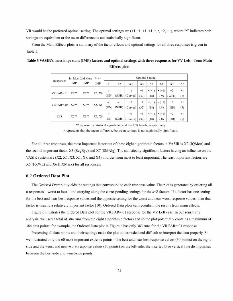
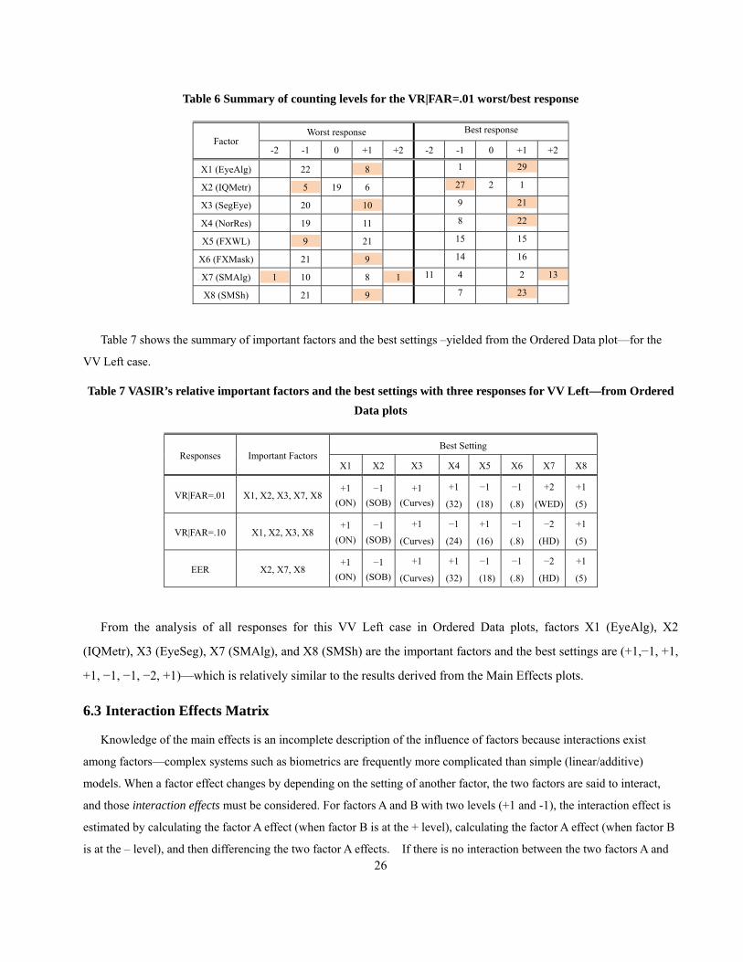
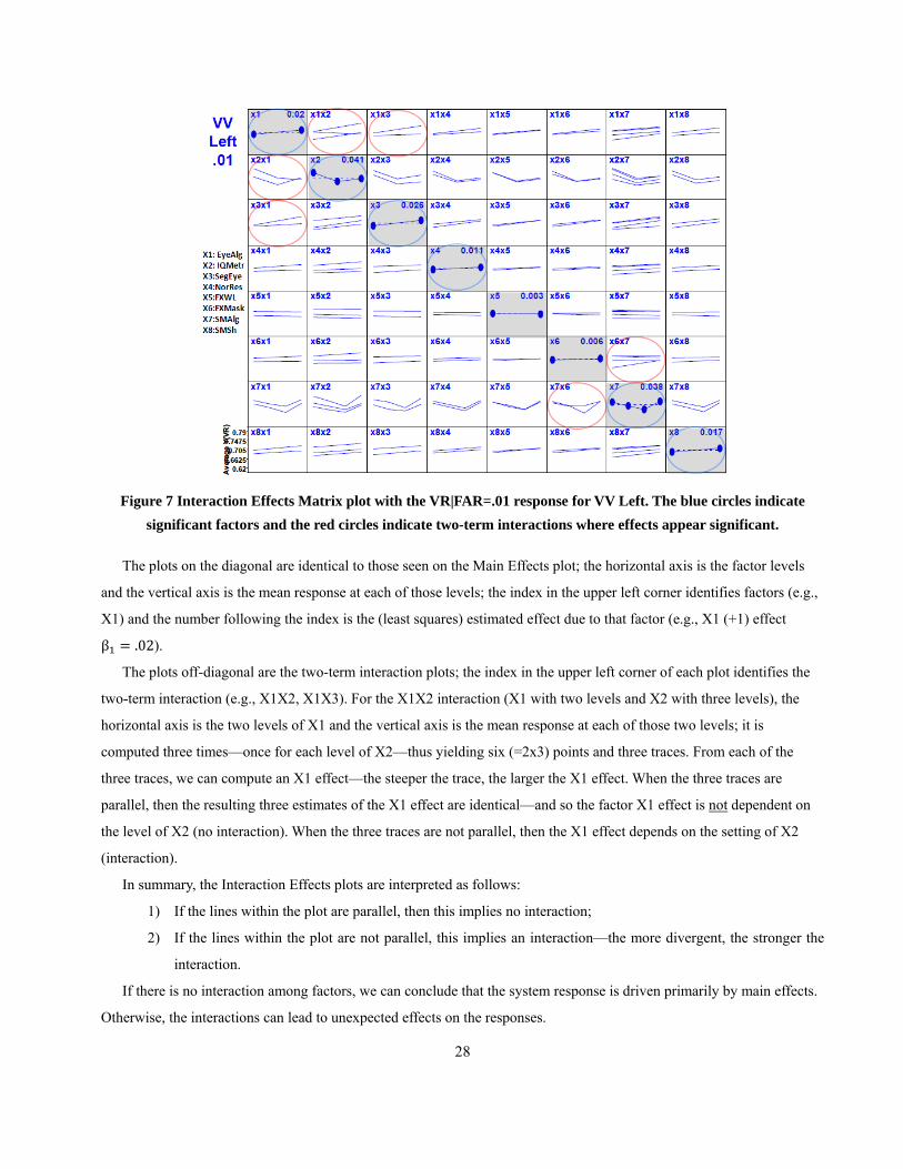
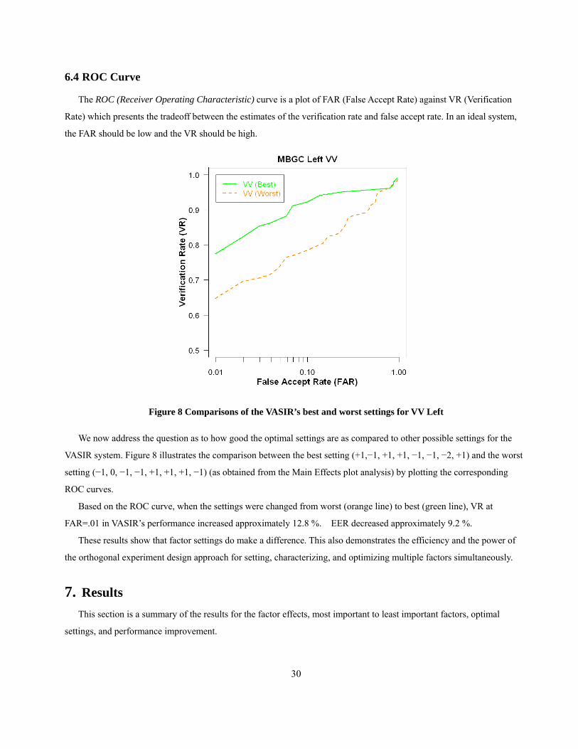
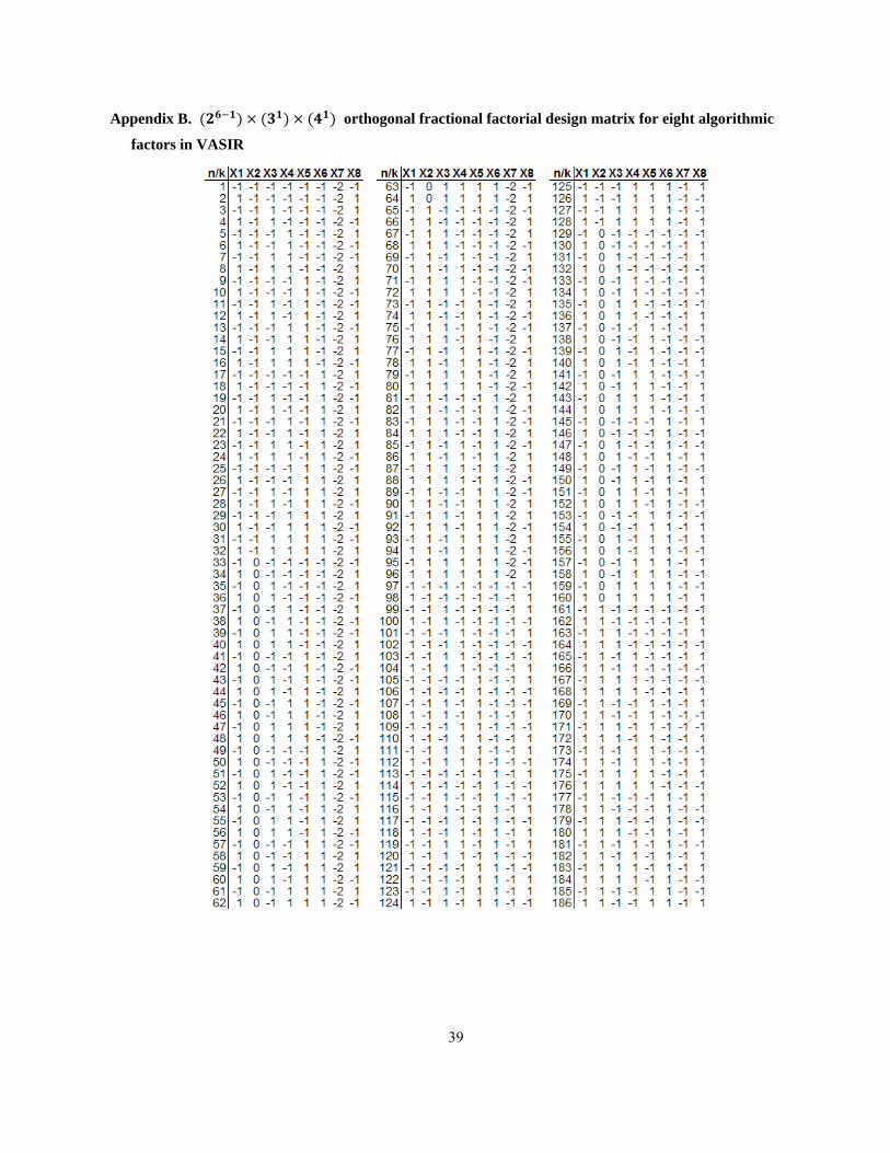
Appendix B ሺሻ ൈ ሺሻ ൈ ሺሻ orthogonal fractional factorial design matrix for eight algorithmic
factors in VASIR
39
40

40


![Biometric Standards documents/Standards... · Biometric Profiles Biometric [Application] Profile – a conforming subset or combination of base standards used to effect specific biometric](https://static.fdocuments.in/doc/165x107/5f711372ce578d4ee02aea91/biometric-standards-documentsstandards-biometric-profiles-biometric-application.jpg)