SENSITIVITY ANALYSIS

NAME: JADHAV CHAITANYA ROLL NO: 26 MMS-II, CHANAKYA

SENSITIVITY ANALYSISThe solution obtained by simplex or graphical method of LP is based

on deterministic assumptions i.e. we assume complete certainty in the data and the relationships of a problem – namely prices are fixed, resources known, time needed to produce a unit exactly etc. However in the real world, conditions are seldom static i.e. they are dynamic. How can such discrepancy be handled? For example if a firm realizes that profit per unit is not Rs 5 as estimated but instead closer to Rs 5.5, how will the final solution mix and total profit change? If additional resources, such as 10 labor hours or 3 hours of machine time, should become available, will this change the problem’s answer? Such analyses are used to examine the effects of changes in these three areas:

1. Contribution rates for each variable – C FACTOR2. Technological coefficients – A FACTOR3. Available Resources – B FACTOR

This task is alternatively called sensitivity analysis. It is also called as post optimality analysis.

Sensitivity analysis often involves a series of what if? questions. What if the profit of product 1 increases by 10%? What if less money is available in advertising budget constraints? What if new technology will allow a product to be wired in one-third the time it used to take? So we can see that sensitivity analysis can be used to deal not only with errors in estimating input parameters to the LP model but also with management’s experiments with possible future changes in the firm that may affect profits.

There are two approaches to determining how sensitive an optimal solution is to changes. The first is simply a trial and error approach, however we prefer the second approach of post optimality method i.e. after an LP problem has been solved, and we attempt to determine a range of changes in problem parameters that will not affect the optimal solution or change the variables in the solution. This is done without resolving the whole problem again. This is illustrated by the following example.

Consider an example of ABC Sound Company that makes CD players (called X1’s) and stereo players (called X2’s). Its LP Formulation is:

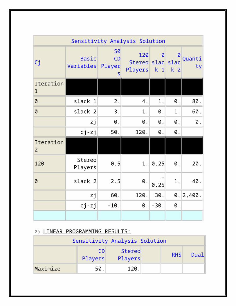
MAXIMIZE PROFIT = $50X1 + $120X2Subject to : 2X1 + 4X2 <= 80 (hour’s of electrician’s time available) 3X1 + 1 X2 <= 60 (hours of audio technician’s time available)1) ITERATIONS:

Sensitivity Analysis Solution

CjBasic

Variables

50 CD

Players

120 Stereo

Players

0 slack

1

0 slack

2Quantity

Iteration 1            

0 slack 1 2. 4. 1. 0. 80.

0 slack 2 3. 1. 0. 1. 60.

  zj 0. 0. 0. 0. 0.

  cj-zj 50. 120. 0. 0.  

Iteration 2            

120Stereo

Players0.5 1. 0.25 0. 20.

0 slack 2 2.5 0. -0.25 1. 40.

  zj 60. 120. 30. 0. 2,400.

  cj-zj -10. 0. -30. 0.  

2) LINEAR PROGRAMMING RESULTS:

Sensitivity Analysis Solution

 CD

PlayersStereo

Players  RHS Dual

Maximize 50. 120.      

Electrician Hrs 2. 4. <= 80. 30.

Audio Tech Hours

3. 1. <= 60. 0.

Solution-> 0. 20.   2,400.  

3) SOLUTION LIST:

Sensitivity Analysis Solution

Variable Status Value

CD Players NON Basic 0.

Stereo Players Basic 20.

slack 1 NON Basic 0.

slack 2 Basic 40.

Optimal Value (Z)   2,400.

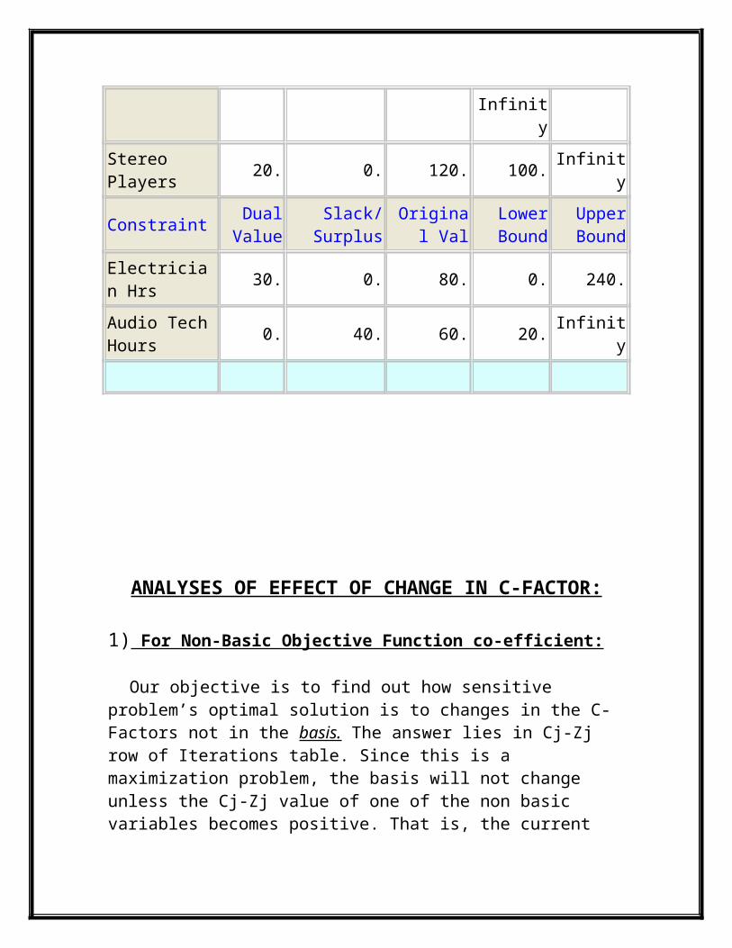
4) RANGE:

Sensitivity Analysis Solution

           

Variable Value Reduced CostOriginal

ValueLower Bound

Upper Bound

CD Players 0. 10. 50. -Infinity 60.

Stereo Players 20. 0. 120. 100. Infinity

ConstraintDual

ValueSlack/Surplus

Original Val

Lower Bound

Upper Bound

Electrician Hrs 30. 0. 80. 0. 240.

Audio Tech Hours

0. 40. 60. 20. Infinity

ANALYSES OF EFFECT OF CHANGE IN C-FACTOR:

1) For Non-Basic Objective Function co-efficient:

Our objective is to find out how sensitive problem’s optimal solution is to changes in the C-Factors not in the basis. The answer lies in Cj-Zj row of Iterations table. Since this is a maximization problem, the basis will not change unless the Cj-Zj value of one of the non basic variables becomes positive. That is, the current solution will be optimal as long as all numbers in the bottom row are less than or equal to zero.

Now Cj-Zj <= 0 is same as Cj <= Zj.

Since X1’s Cj value is Rs.50 and its Zj value is Rs.60, the current solution is optimal as long as the profit per CD does not exceed Rs.60, or does not increase by Rs.10. Similarly the C-Factor for S1 (per hour of electrician’s time) may increase from Rs.0 to Rs.30 without changing the current solution mix. In other words any change in the C-Factor for Non-Basic Objective Function co-efficient:

Affects only coefficient in the Cj-Zj row under the column of the variable whose objective coefficient is being changed.

Does not affect profit.

2) For Basic Objective function co-efficient:

Let us consider changing the C-Factor of stereo players by Δ. A change in C-Factor will affect the Cj-Zj values of all non basic variables because this Cj is not only in Cj row but Cj column. This then impacts the Zj row.

When we examine the S1 column in the table below:-30 – ¼ Δ <= 0

-30 <= ¼ Δ-120 <= Δ or Δ >= -120.

This implies that S1 is less sensitive to change than X1. S1 will not enter the basis unless the C-Factor drops from Rs.120 to 0. In other words any change in the C-Factor for Basic Objective function co-efficient:

Affects only the coefficients in the Zj row and Zj-Cj row under the columns of the non basic variables.

Affects Profit. The revised profit = (Profit before change + Δ * coefficient in the constraint row of the variable whose objective function is being changed.)

Sensitivity Analysis Solution

CjBasic

Variables

50 CD

Players

120 + Δ Stereo

Players

0 slack 1

0 slack

2Quantity

Iteration 1            

0 slack 1 2. 4. 1. 0. 80.

0 slack 2 3. 1. 0. 1. 60.

  zj 0. 0. 0. 0. 0.

  cj-zj 50. 120 + Δ. 0. 0.  

Iteration 2            

120 + ΔStereo

Players0.5 1. 0.25 0. 20.

0 slack 2 2.5 0. -0.25 1. 40.

  zj 60 + ½ Δ. 120 + Δ.30 + ¼ Δ.

0.2,400 + 20 Δ.

  cj-zj -10- ½ Δ. 0.-30 – ¼

Δ.0.  

ANALYSES OF EFFECT OF CHANGE IN B-FACTOR:

This leads us to the concept of shadow price i.e. the value of one additional unit of a scarce resource which provides important economic information. The negative of the numbers in the Cj-Zj row’s slack variable columns are the shadow prices. In this case the Cj-Zj row’s S1 Column is (-30) which suggests that the additional cost of one electrician hour should not exceed Rs.30. Similarly since Cj-Zj row’s S2 column is 0, it suggests that the audio technician hours are under utilized.

Now we cannot add an unlimited number of units of resources without eventually violating one of the problem’s constraints. So let’s determine the range of shadow prices i.e. RIGHT HAND SIDE RANGING.

Quantity S1 RATIO20 1/4 20/(1/4) = 8040 -1/4 40/(1/4) = -160

From the above table it’s clear that we can decrease the electrician’s time resource by 80 hours i.e. to 0 hours or increase it by 160 hours i.e. to 240 hours without affecting the current solution’s mix. If it is increased by a value beyond this range say Δ it will:

Affect the values in the solution column of the optimal simplex tableau.

Affect the profit. The revised profit = (Profit before change + Δ * corresponding element in the Zj row and Cj-Zj row under the column of slack variable of the resource whose availability is changed.)