Sensing Our Planet

NASA Earth Science Research Features 2011

National Aeronautics and Space Administration

Sensing Our PlanetNASA Earth Science Research Features 2011

National Aeronautics and Space Administration

NASA Earth Observing System Data and Information System (EOSDIS) Data Centers

www.nasa.gov

Front cover imagesTop row, left to right:

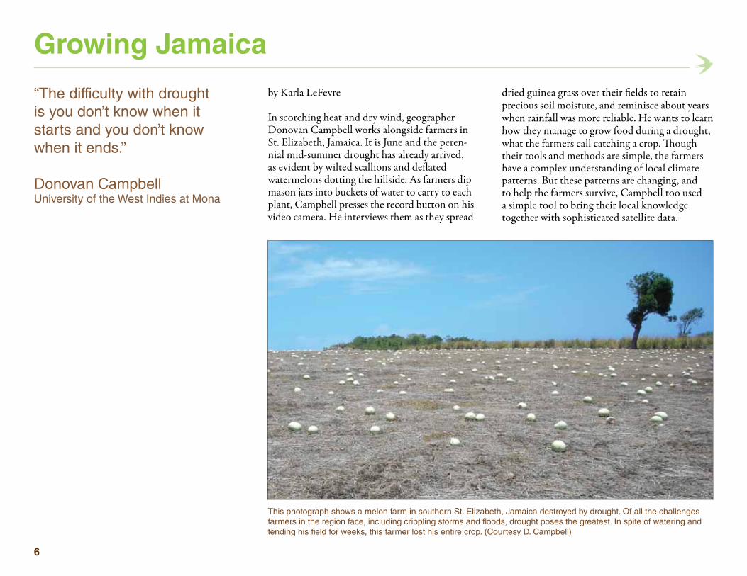
This photograph shows a melon farm in southern St. Elizabeth, Jamaica destroyed by drought. Of all the challenges farmers in the region face, including crippling storms and floods, drought poses the greatest. In spite of watering and tending his field for weeks, this farmer lost his entire crop. See the related article, “Growing Jamaica,” on page 6. (Courtesy D. Campbell)

The Gunnison sage-grouse lives in isolated portions of Colorado and Utah. Its former range, extending into Arizona and New Mexico, was whittled down by energy develop-ment, cattle grazing, and invasive weeds that disturbed the sagebrush habitat on which the grouse survives. This male grouse is in full strut, fanning his tail feathers and inflat-ing the air sacs on his chest. See the related article, “The feather followers,” on page 32. (Courtesy G. Vyn)

The city of Cairo is barely visible behind the pyramids in this photograph, due to the heavy layer of haze. See the related article, “A black cloud over Cairo,” on page 18. (Courtesy P. Medved)

A man stands in the middle of the Karakoram Highway while rocks tumble down into the Hunza River in Pakistan’s Gojal region. The rockslide dammed the river and created Lake Gojal, which submerged eleven miles of the Karakoram Highway and isolated several villages. See the related article, “Waiting for Gojal,” on page 2. (Courtesy I. Ali [Shimshal]/Pamir Times)

Bottom row, left to right:

In the fall, trees in this deciduous forest in Northumberland County, Ontario, Canada start to change colors and lose their leaves. As the seasons change from summer to winter, forests slow down their growth and absorb much less carbon from the atmosphere. See the related article, “Hidden carbon,” on page 36. (Courtesy D. Cronin)

The Advanced Spaceborne Thermal Emission and Reflection Radiometer (ASTER) on the NASA Terra satellite acquired this image of Umiamiko Glacier in Greenland. Researchers have observed rapid melt of the Greenland Ice Sheet and its glaciers in recent years, adding water to the world’s oceans. See the related article, “The un-ice age,” on page 22. (Courtesy J. Box and I. Howat/ASTER)

Early-morning lenticular and stratus clouds form over the foothills in Boulder, Colorado. High-rate Global Positioning System (GPS) receivers, such as the one in the foreground, can help scientists detect the amount of moisture in the soil, which improves weather and flood forecasting. See the related article, “Looking for mud,” on page 40. (Courtesy N. Vizcarra)

Back cover imagesTop row, left to right:

People built these terraces to grow rice, in the Cordillera Mountains, north of Manila in the Philippines. They are one example of how humans have transformed ecologies around the world. See the related article, “Repatterning the world,” on page 14. (Courtesy S. Ciencia)

Pilots Shane Dover (left), Bill Brockett (right), and other NASA pilots flew the NASA DC-8 and the Genesis and Rapid Intensification Process (GRIP) scientists on sixteen science flights in just less that two months from their temporary base in Ft. Lauderdale, Florida. The flight crew and scientists also made three deployments from St. Croix, U.S. Virgin Islands to extend their range farther east over the Atlantic Ocean. (Courtesy S. Smith/LaRC)

Bottom row, left to right:

Much of the bluish mist shrouding the Great Smoky Mountains in the southeastern United States is caused when trees emit chemicals into the atmosphere. In large amounts these chemicals form a visible haze. See the related article, “Volatile trees,” on page 48. (Courtesy F. Kehren)

In the early 2000s biologists discovered that microscopic crustaceans called copepods carried cholera bacteria in their guts. These copepod illustrations were drawn in the mid-1800s by German biologist Ernst Haeckel. See the related article, “The time of cholera,” on page 10.

The April 2010 El Mayor-Cucapah earthquake revealed a previously undiscovered fault in the desert of Baja California, Mexico. Although the fault is relatively small, it produced a magnitude 7.2 earthquake. Scientists have become interested in smaller faults, because they are frequently the location of unexpectedly large earthquakes. See the related article, “Baja’s fault,” on page 44. (Courtesy T. Fletcher)

ii

About the EOSDIS data centersThe articles in this issue arose from research that used data from NASA Earth Observing System Data and Information System (EOSDIS) data centers. The data centers, managed by NASA’s Earth Science Data and Information System Project (ESDIS), offer more than 4,000 Earth system science data products and associated services to a wide community of users. ESDIS develops and operates EOSDIS, a distributed system of data centers and science investigator processing systems. EOSDIS processes, archives, and distributes data from Earth observing satellites, field campaigns, airborne sensors, and related Earth science programs. These data enable the study of Earth from space to advance scientific understanding.

For more information“About the NASA Earth Observing System Data Centers” (page 52)NASA Earth Data Web site http://earthdata.nasa.govNASA Earth Science Web site http://science.nasa.gov/earth-science

Land Processes DAACSurface Reflectance, Land Cover, Vegetation Indices

National Snow and Ice Data Center DAAC

Snow and Ice, Cryosphere, Climate Interactions, Sea Ice

Physical Oceanography DAAC

Gravity, Sea Surface Temperature, Ocean Winds, Topography,

Circulation, Currents

Alaska Satellite Facility SAR Data Center

SAR Products, Sea Ice,Polar Processes,

Geophysics

Socioeconomic Data and Applications CenterHuman Interactions, Land Use, Environmental Sustainability, Geospatial Data

Ocean Biology Processing GroupOcean Biology, Sea Surface Temperature

Crustal Dynamics Data Information SystemSpace Geodesy, Solid Earth

MODAPS Level 1 and Atmosphere Archive and Distribution SystemMODIS Level 1 and Atmosphere Data Products

Goddard Earth Sciences Data and Information Services CenterGlobal Precipitation,Solar Irradiance, Atmospheric Composition and Dynamics, Global Modeling

iii

Langley Research Center Atmospheric Science Data CenterRadiation Budget, Clouds, Aerosols, Tropospheric Chemistry

Oak Ridge National Laboratory DAACBiogeochemical Dynamics, Ecological Data, Environmental Processes

Global Hydrology Resource CenterHydrologic Cycle, Severe Weather Interactions, Lightning, Atmospheric Convection

About Sensing Our PlanetEach year, Sensing Our Planet features intriguing research that highlights how scientists are using Earth science data to learn about our planet. These articles are also a resource for learning about science and about the data, for discovering new and interdiscipli-nary uses of science data sets, and for locating data and education resources.

Articles and images from Sensing Our Planet: NASA Earth Science Research Features 2011 are available online at the NASA Earth Data Web site (http://earthdata.nasa.gov/sensing-our-planet/). A PDF of the full publication is also available on the site.

For additional print copies of this publication, please e-mail nsidc@nsidc.org.

Researchers working with EOSDIS data are invited to e-mail the editors at eosdis.editor@nsidc.org with ideas for future articles.

The design featured in this issue represents a soaring swallow. Several stories for 2011 spotlight how satellite and ground observations can help steward natural resources. See “Growing Jamaica” on page 6; “Repatterning the world” on page 14; and “The feather followers” on page 32.

AcknowledgementsThis publication was produced at the Snow and Ice Distributed Active Archive Center (DAAC), at the National Snow and Ice Data Center, under NASA GSFC contract No. NNG08HZ07C, awarded to the Cooperative Institute for Research in Environmental Sciences at the University of Colorado Boulder. We thank the EOSDIS data center managers and personnel for their direction and reviews, and the scientists who alerted us to recent research that made use of EOSDIS data.

We especially thank our featured investigators for their time and assistance.

Writing, editing, and designEditor: Jane BeitlerAssistant Editor: Natasha VizcarraWriters: Jane Beitler, Karla LeFevre, Katherine Leitzell, Laura Naranjo, and Natasha VizcarraPublication Design: Laura Naranjo

Printing notesPrinted with vegetable-based inks at a facility certified by the Forest Stewardship Council; uses 30 percent recycled chlorine-free paper that is manufactured in the U.S.A. with electricity offset by renewable energy certificates.

iv

Made in

U. S. A.

Sensing Our PlanetNASA Earth Science Research Features 2011

Waiting for Gojal 2Scientists and satellites hold vigil on a newborn lake in Pakistan.

Growing Jamaica 6Local knowledge plus satellites may help farmers catch a crop.

The time of cholera 10The color of water could be a tool for heading off epidemics.

Repatterning the world 14As wildlands shrink, scientists study the ecologies that people have tamed.

A black cloud over Cairo 18The source of a yearly scourge is revealed.

The un-ice age 22Earth’s remaining ice sheets head for the ocean.

Once more into the storm 28Hurricane researchers return, asking new questions.

The feather followers 32Many eyes help protect the birds they love to watch.

Hidden carbon 36Satellites measure the give and take between trees and temperatures.

Looking for mud 40Scientists stumble on a weird way to measure the moisture in soil.

Baja’s fault 44Before and after images trace an earthquake’s surprise.

Volatile trees 48Forests fill the air with more than just a fresh scent.

2

by Natasha Vizcarra

A nervous sense of humor greets travelers at the highest and most scenic road in the world. Hand-painted signs saying, “Relax, slide area ends” dot sections of the Karakoram Highway along the Hunza River in northern Pakistan. Landslides are commonplace here. But on January 4, 2010, a massive rockslide buried

part of a village and blocked the river’s flow. Boulders, rocks, and debris tumbled down the mountainside that day, killing twenty people and damming the river until it swelled and swallowed more communities. In months, the plugged-up river would submerge eleven miles of the Karakoram Highway, turning a thriving region buzzing with trade from the Chinese border into scattered clumps of unconnected villages.

Waiting for Gojal

A man stands in the middle of the Karakoram Highway while rocks tumble down into the Hunza River in Pakistan’s Gojal region. The rockslide dammed the river and created Lake Gojal, which submerged eleven miles of the Karakoram Highway and isolated several villages. (Courtesy I. Ali [Shimshal]/Pamir Times)

“It’s always startling to see the first images of these kinds of things.”

Gregory LeonardUniversity of Arizona

3

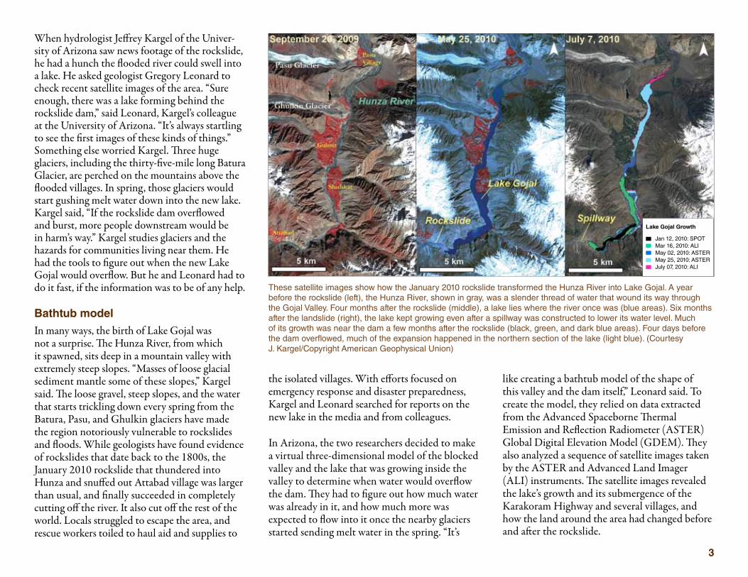
When hydrologist Jeffrey Kargel of the Univer-sity of Arizona saw news footage of the rockslide, he had a hunch the flooded river could swell into a lake. He asked geologist Gregory Leonard to check recent satellite images of the area. “Sure enough, there was a lake forming behind the rockslide dam,” said Leonard, Kargel’s colleague at the University of Arizona. “It’s always startling to see the first images of these kinds of things.” Something else worried Kargel. Three huge glaciers, including the thirty-five-mile long Batura Glacier, are perched on the mountains above the flooded villages. In spring, those glaciers would start gushing melt water down into the new lake. Kargel said, “If the rockslide dam overflowed and burst, more people downstream would be in harm’s way.” Kargel studies glaciers and the hazards for communities living near them. He had the tools to figure out when the new Lake Gojal would overflow. But he and Leonard had to do it fast, if the information was to be of any help.

Bathtub model

In many ways, the birth of Lake Gojal was not a surprise. The Hunza River, from which it spawned, sits deep in a mountain valley with extremely steep slopes. “Masses of loose glacial sediment mantle some of these slopes,” Kargel said. The loose gravel, steep slopes, and the water that starts trickling down every spring from the Batura, Pasu, and Ghulkin glaciers have made the region notoriously vulnerable to rockslides and floods. While geologists have found evidence of rockslides that date back to the 1800s, the January 2010 rockslide that thundered into Hunza and snuffed out Attabad village was larger than usual, and finally succeeded in completely cutting off the river. It also cut off the rest of the world. Locals struggled to escape the area, and rescue workers toiled to haul aid and supplies to

the isolated villages. With efforts focused on emergency response and disaster preparedness, Kargel and Leonard searched for reports on the new lake in the media and from colleagues.

In Arizona, the two researchers decided to make a virtual three-dimensional model of the blocked valley and the lake that was growing inside the valley to determine when water would overflow the dam. They had to figure out how much water was already in it, and how much more was expected to flow into it once the nearby glaciers started sending melt water in the spring. “It’s

like creating a bathtub model of the shape of this valley and the dam itself,” Leonard said. To create the model, they relied on data extracted from the Advanced Spaceborne Thermal Emission and Reflection Radiometer (ASTER) Global Digital Elevation Model (GDEM). They also analyzed a sequence of satellite images taken by the ASTER and Advanced Land Imager (ALI) instruments. The satellite images revealed the lake’s growth and its submergence of the Karakoram Highway and several villages, and how the land around the area had changed before and after the rockslide.

These satellite images show how the January 2010 rockslide transformed the Hunza River into Lake Gojal. A year before the rockslide (left), the Hunza River, shown in gray, was a slender thread of water that wound its way through the Gojal Valley. Four months after the rockslide (middle), a lake lies where the river once was (blue areas). Six months after the landslide (right), the lake kept growing even after a spillway was constructed to lower its water level. Much of its growth was near the dam a few months after the rockslide (black, green, and dark blue areas). Four days before the dam overflowed, much of the expansion happened in the northern section of the lake (light blue). (Courtesy J. Kargel/Copyright American Geophysical Union)

Lake Gojal Growth

Jan 12, 2010: SPOT Mar 16, 2010: ALI May 02, 2010: ASTER May 25, 2010: ASTER July 07, 2010: ALI

4

A swelling lake They now knew what the shape of the tub looked like; the next challenge was to gauge how much water was flowing into it. Kargel found a thirty-year record of the Hunza River’s rate of flow. “That data set was really crucial,” he said. With it, they could estimate how much water was flowing into the lake, and how the lake would evolve. To identify the sources of glacier melt water above the valley, they used images from the Global Land Ice Measurements from Space (GLIMS) project. But they still needed to confirm some of the river flow and satellite data with field observations. Geoscientist Jean Schneider was already at Lake Gojal, working as a consultant for Pakistan’s National Disaster Management Authority (NDMA). He described what kind of rocks and soil had tumbled from the mountainside, measured everything that he could, and sent photographs. “Internet access was difficult in the region, so it was hard to get data to and from Jeffrey in the field,” said Schneider, who had to send the data from his office at the University of Vienna.

The researchers calculated that the lake’s volume was three to four times larger than what was being reported by the local media. They predicted on April 14, 2010, that the lake would overflow sometime from May 29 to June 1, and that there was a possibility that the rockslide dam would burst. “I was a little alarmed at the difference in our figures and what was being reported,” Kargel said. “So I approached the U.S. State Department’s Pakistan office, retired Pakistan military authorities who were still connected to the Pakistan NDMA, and I approached Focus Humanitarian Assistance Pakistan. These urgent warnings apparently did reach the authorities in the field and presumably were of some use in planning and preparations for a possible flood.”

From mid-winter to late spring, disaster management crews had been carving out a spill-way to ease the lake’s swelling, and evacuating communities. The growing lake had displaced more than a thousand people and destroyed homes, farms, and fruit orchards in the villages of Shishkat and Gulmit. As it turned out, the overflow began on May 29, and the spilling water soon grew to a torrent.

Forever or not

To the researchers’ surprise, the dam held as the water spilled over. Kargel said, “Everybody concerned, with one exception, was expecting a catastrophe of one magnitude or another.” That exception was hydrologist Victor Baker, Kargel’s colleague at the University of Arizona. Baker was convinced that the dam would hold and that the new lake would remain a lake for many years. “He believed that the dam’s downstream length was long enough and massive enough to prevent a rapid outburst,” Kargel said. The energy from water spilling over would be dissipated as

it traversed the almost mile-long dam and would keep villages downstream safe. The lake would drain slowly and carve out a natural spillway through gradual erosion.

“Indeed, Baker has so far been correct,” Kargel said. However, Kargel and Leonard are not convinced that the lake is completely harmless. The rockslide dam contains clay from previous glacier melts and landslide-dammed lakes in the valley. Kargel believes the clay could deform over winters and springs as water inside it repeatedly freezes and thaws. Water seeping from within the dam might erode the clay and cause a catastrophic dam burst. Leonard said rockslide dams also typically burst shortly after an overflow. “This really is a big question,” he said. “We all wonder if this one is going to last a long time.”

Waiting game

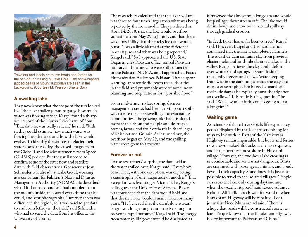
As scientists debate Lake Gojal’s life expectancy, people displaced by the lake are scrambling for ways to live with it. Parts of the Karakoram Highway remain impassable, but boats and ferries now crowd makeshift docks at the lake’s spillway and at the northernmost shore in Hussaini village. However, the two-hour lake crossing is uncomfortable and somewhat dangerous. Boats are crammed with passengers, animals, and goods beyond their capacity. Sometimes, it is just not possible to travel to the isolated villages. “People can cross the lake only during daytime and when the weather is good,” said rescue volunteer Rehmat Ali Tajik. Locals wait for word of when Karakoram Highway will be repaired. Local journalist Noor Muhammad said, “There is a hope that roads will be constructed sooner or later. People know that the Karakoram Highway is very important to Pakistan and China.”

Travelers and locals cram into boats and ferries for the two-hour crossing of Lake Gojal. The snow-capped, jagged peaks of Mount Tupopdan are seen in the background. (Courtesy M. Pearson/ShelterBox)

5

Meanwhile, the lake needs watching. Locals fear that Lake Gojal still holds a dangerous amount of water and have used hand tools to widen the spillway themselves. “The spillway has just not been able to bring the water level down considerably,” Muhammad said. Unusually warm weather could bring more water from the glaciers down to the lake. Kargel and his colleagues continue to distrust the dam. “The lake remains dangerous, in my opinion,” Kargel said. “We will keep a satellite’s eye view on the situation.” It may turn out to be a long vigil. “This lake could go at any time, or it could just last for centuries,” he said.

To access this article online, please visit http://earthdata.nasa .gov/featured-stories/featured-research/waiting-gojal

Reference Kargel, J. S. and G. Leonard. 2010. Satellite monitoring of Pakistan’s rockslide-dammed Lake Gojal. Eos, Transactions, American Geophysical Union 91 (43):394-395.

For more informationNASA Land Processes Distributed Active Archive Center (LP DAAC) https://lpdaac.usgs.govNASA National Snow and Ice Data Center (NSIDC) DAAC http://nsidc.org Advanced Spaceborne Thermal Emission and Reflection Radiometer (ASTER) http://asterweb.jpl.nasa.govEarth Observing-1 Advanced Land Imager http://edcsns17.cr.usgs.gov/eo1/sensors/aliGlobal Land Ice Measurements from Space (GLIMS) http://www.glims.org

About the scientists

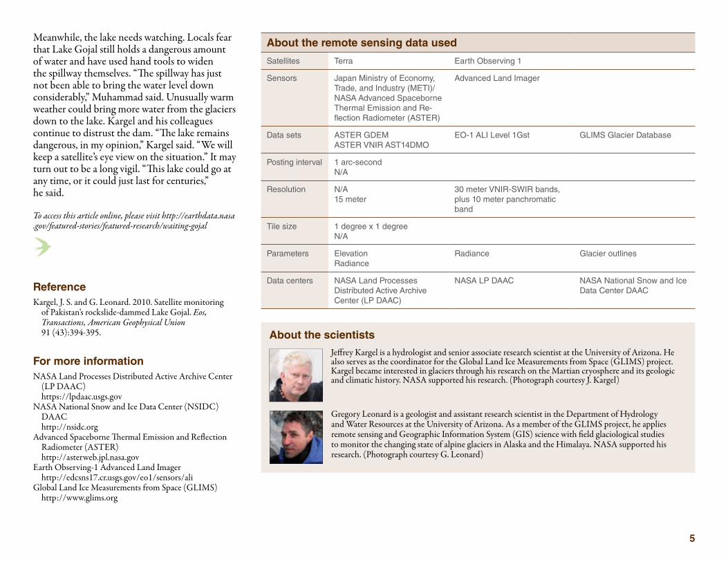
Jeffrey Kargel is a hydrologist and senior associate research scientist at the University of Arizona. He also serves as the coordinator for the Global Land Ice Measurements from Space (GLIMS) project. Kargel became interested in glaciers through his research on the Martian cryosphere and its geologic and climatic history. NASA supported his research. (Photograph courtesy J. Kargel)

Gregory Leonard is a geologist and assistant research scientist in the Department of Hydrology and Water Resources at the University of Arizona. As a member of the GLIMS project, he applies remote sensing and Geographic Information System (GIS) science with field glaciological studies to monitor the changing state of alpine glaciers in Alaska and the Himalaya. NASA supported his research. (Photograph courtesy G. Leonard)

About the remote sensing data used

Satellites Terra Earth Observing 1

Sensors Japan Ministry of Economy, Trade, and Industry (METI)/NASA Advanced Spaceborne Thermal Emission and Re-flection Radiometer (ASTER)

Advanced Land Imager

Data sets ASTER GDEMASTER VNIR AST14DMO

EO-1 ALI Level 1Gst GLIMS Glacier Database

Posting interval 1 arc-secondN/A

Resolution N/A15 meter

30 meter VNIR-SWIR bands, plus 10 meter panchromatic band

Tile size 1 degree x 1 degreeN/A

Parameters ElevationRadiance

Radiance Glacier outlines

Data centers NASA Land Processes Distributed Active Archive Center (LP DAAC)

NASA LP DAAC NASA National Snow and Ice Data Center DAAC

6

by Karla LeFevre

In scorching heat and dry wind, geographer Donovan Campbell works alongside farmers in St. Elizabeth, Jamaica. It is June and the peren-nial mid-summer drought has already arrived, as evident by wilted scallions and deflated watermelons dotting the hillside. As farmers dip mason jars into buckets of water to carry to each plant, Campbell presses the record button on his video camera. He interviews them as they spread

dried guinea grass over their fields to retain precious soil moisture, and reminisce about years when rainfall was more reliable. He wants to learn how they manage to grow food during a drought, what the farmers call catching a crop. Though their tools and methods are simple, the farmers have a complex understanding of local climate patterns. But these patterns are changing, and to help the farmers survive, Campbell too used a simple tool to bring their local knowledge together with sophisticated satellite data.

Growing Jamaica

This photograph shows a melon farm in southern St. Elizabeth, Jamaica destroyed by drought. Of all the challenges farmers in the region face, including crippling storms and floods, drought poses the greatest. In spite of watering and tending his field for weeks, this farmer lost his entire crop. (Courtesy D. Campbell)

“The difficulty with drought is you don’t know when it starts and you don’t know when it ends.”

Donovan CampbellUniversity of the West Indies at Mona

7

Ground-level knowledge Hoping to study how farmers cope with drought, and to bring science to bear on their situation, Campbell relocated from the University of the West Indies in Kingston to St. Elizabeth in 2007. A native Jamaican from a rural family, Campbell conversed with them in Patois, a creole language that is spoken in many farming communities, but is rarely written. He focused on farmers who tend three acres or less. Their small-scale farms are the backbone of domestic food production. But their farms are in danger of disappearing, pummeled by years of drought, water costs that doubled in just two years, plus higher prices for supplies, like mulch and fertilizer. Such problems all but blotted out Jamaican onion farms in three years, with 800 hectares (2,000 acres) dwindling to a handful by 1999.

Of all these problems, drought is the hardest to solve. To make matters worse, the farmers have noticed the mid-summer drought arriving earlier and sticking around longer. What once seemed extreme, they said, has become the norm. Campbell wondered if he could capture their view in scientific data. He said, “These farmers have lived in the area for many, many decades, so they are more familiar with the conditions than any scientist.” But if scientific measurements also pointed to changing climate patterns, it might help shape solutions or even bring govern-ment attention to the situation. So he set about to learn what the farmers experienced, and to find if there were data to support their intuitions.

Shrouded in shadow Jamaica’s breadbasket is nestled in the southern section of St. Elizabeth Parish, one of the island’s fourteen subdivided counties, where over 70 percent of people depend on farming for their

livelihood. Fresh scallion, sweet peppers, melons, and cassava—a root tuber ground into flour and used for making bammies, or flatbread—have fed Jamaicans for generations. Steep farmlands run south from the slopes of the Santa Cruz Moun-tains to the rocky coast of the Caribbean Sea. As one farmer explained to Campbell, “[Farming] is not a bed of roses these days, but for most of us here in St. Elizabeth, farming is the only thing we know. It is in our blood.”

Ironically, this breadbasket sits in a rain shadow and receives less rainfall than the rest of the island. When prevailing winds flow northeast from the Atlantic across Jamaica, they bring moist, warm air necessary for forming rain clouds. But the Santa Cruz Mountains block the passage of the prevailing winds and the rain systems they bring, leaving southern St. Elizabeth on the dry side of the mountains.

Talking to the farmers, Campbell learned that they have honed a complex crop schedule over many decades to fit the local climate. Two dry seasons, one in July and one from December through March, interrupt the growing season. So they plant quick-growing crops for April through June, and this early-season harvest finances their late-season cash crops, which they grow from August through November. The cash crop season also coincides with the main hurricane season, which can bring crippling storms and floods.

Even so, drought poses a greater challenge, particularly for small-scale farmers who lack running water and irrigation systems. Campbell said, “The difficulty with drought is you don’t know when it starts and you don’t know when it ends.” So when the dry season arrives, they must tap into limited reserves of water stored in shared

A hearty 75-year-old farmer in southern St. Elizabeth, Jamaica prepares his field for planting his next crop of potatoes. (Courtesy D. Campbell)

8

stone water tanks, called catchments, and eventu-ally into limited reserves of cash to have these catchments refilled. They also have to pay for more guinea grass mulch in an attempt to lock in soil moisture, and for more fertilizer to coax their ailing crops along. “So a farmer will expend a lot of his resources during a drought,” Campbell said. And when below-average rainfall turns the dry season into an extended drought, Jamaica’s shallow aquifers quickly dry up, too, leaving everyone’s buckets and mason jars empty.

Verifying local observations Campbell needed a long series of rainfall records to show that patterns had truly changed. The challenge was finding those records. Farmers’ memories of weather events stretched back

thirty years or more, but local land-based rain gauge measurements provided spotty data, and for just five to ten years. So he worked with climatologists Doug Gamble at the University of North Carolina Wilmington and Scott Curtis at East Carolina University to obtain satellite data. At the Goddard Earth Sciences Data and Information Services Center (GES DISC), they found Tropical Rainfall Measuring Mission (TRMM) satellite data and a visualization tool called Giovanni that simplified the process of getting and using rainfall data for St. Elizabeth. Curtis said, “You can get the data you want without being overloaded with megabytes of data. And the TRMM data have a fine time and space scale that allows you to zoom in on a particular parish.”

First the team studied average monthly rainfall maps online for the entire island, then focused in on St. Elizabeth in 25 kilometer (16 mile) square chunks. The TRMM record was complete. It provided over thirty years of daily rainfall data, and included other satellite data to fill any gaps. The researchers found that drought events have indeed become more frequent and severe over the past twenty years. Gamble said, “What’s most interesting is, if you look at the overall trend of rainfall, yes, there’s a decrease, but that’s not the real story.”

The team made a breakthrough when they looked at the data through the farmers’ eyes. Gamble said, “If we hadn’t talked to the farmers and realized how important the early season is, we wouldn’t have broken it into an early sea-son and a late season.” Most previous work had focused on the intensity and length of drought as the most threatening factors to crops. But for farmers, timing is critical. Misjudging a season by one week can undermine their ability to bring a mature crop to market, and to finance their next growing season. “So it made us look at the data in a different way and we found something very important, that drought is much more prevalent at the beginning of the year,” Gamble said.

Hope of relief But if the Jamaican government or relief organizations could help these farmers, when would they step in? The data on drought timing provided the answer. Gamble said, “We validated what the farmers said and it gives us a nice foundation. It gives us a way to not only address drought, but to address the early drought as compared to the later drought.” Supplemental water delivery to farmers during this critical time, for example, could provide substantial relief. Campbell said, “So it shows you that what the

To understand how drought affects farmers in St. Elizabeth, Jamaica, scientists compared farmers’ local knowledge of rainfall patterns with rainfall data from the Tropical Rainfall Measuring Mission (TRMM) satellite. This TRMM data image shows the spatial distribution of rain in millimeters per hour over Jamaica from May 1998 through May 2010. Red, orange, and yellow areas received the most rain. (Courtesy D. Campbell/NASA GES DISC)

18.6N

18.5N

18.4N

18.3N

18.2N

18.1N

18N

17.9N

17.8N

78.4W 78.2W 78W 77.8W 77.6W 77.4W 77.2W 77W 76.8W 76.6W 76.4W 76.2W

0.08841 0.10722 0.12604 0.14485 0.16367 0.18248

Jamaica

St. Elizabeth Parish

Kingston

Montego Bay

Black River

9

farmers are experiencing in these communities is where we should be focusing our research.”

Yet larger questions still loom. What are the best options for helping farmers adapt? Will drought get even worse in the future? To build a clear picture, Campbell continues to work with farmers and is expanding the study area to other agricultural regions in Jamaica. Meanwhile, Gamble and Curtis are busy analyzing satellite vegetation data to understand how drought affects local crops. The team plans to outfit fields with rain gauges and involve farmers in active climate monitoring. They hope that, by strength-ening the view from space with what the farmers see in their fields, these questions too will be answered. Gamble said, “I can find a trend within that satellite data, but if the farmers aren’t worried about it, then that trend doesn’t matter.”

To access this article online, please visit http://earthdata.nasa .gov/sensing-our-planet/2011/growing-jamaica

References Allen, T., S. Curtis, and D. Gamble. 2010. The mid-summer dry spell’s impact on vegetation in Jamaica. Journal of Applied Meteorology and Climatology, doi:10.1175/2010JAMC2422.1.Campbell, D., D. Barker, and D. McGregor. 2011. Dealing with drought: Small farmers and environmental hazards in southern St. Elizabeth, Jamaica. Applied Geography 31 (1):146-158, Hazards, January 2011, ISSN 0143-6228, doi:10.1016/j.apgeog.2010.03.007.Gamble, D. W., D. Campbell, T. L. Allen, D. Barker, S. Curtis, D. McGregor, and J. Popke. 2010. Climate change, drought, and Jamaican agriculture: local knowledge and the climate record. Annals of the Association of American Geographers 100 (4):880-893.

For more informationNASA Goddard Earth Sciences Data and Information Services Center (GES DISC) http://daac.gsfc.nasa.govTropical Rainfall Measuring Mission (TRMM) http://trmm.gsfc.nasa.govGES DISC Interactive Online Visualization and Analysis Infrastructure (Giovanni) Web Site http://disc.sci.gsfc.nasa.gov/giovanni

Donovan Campbell http://www.mona.uwi.edu/geoggeol/staff/ dcampbell.htmScott Curtis http://www.ecu.edu/sustainabletourism/ Scott-Curtis.cfmDouglas W. Gamble http://uncw.edu/earsci/PeopleGamble.htm

About the scientists

Donovan Campbell is a PhD candidate at the University of West Indies at Mona. His current research focuses on natural hazards and domestic food production to understand how farmers cope with climatic variability and change. Campbell’s main research objective is to understand how small-scale food producers in the Caribbean adapt to changes occurring in their environment. The National Science Foundation supported his research. (Photograph courtesy D. Campbell)

Douglas W. Gamble is an associate professor and the director of the Laboratory for Applied Climate Research at the University of North Carolina Wilmington. His current research includes the hydro-climatology of the Caribbean and the perception of climate change in Jamaica and the Bahamas. The National Science Foundation supported his research. (Photograph courtesy D. Gamble)

Scott Curtis is an associate professor and assistant director of the Center for Natural Hazards Research at East Carolina University. His current work includes precipitation extremes, climate variability, global satellite data analysis, weather-climate-tourism, and drought in the Caribbean. The National Science Foundation supported his research. (Photograph courtesy S. Curtis)

About the remote sensing data used

Satellite Tropical Rainfall Measuring Mission (TRMM)

Sensor TRMM Microwave Imager

Data set TRMM Level 3 Monthly Data Products

Resolution 25 degree

Parameter Precipitation

Data center NASA Goddard Earth Sciences Data and Information Services Center (GES DISC)

The images and data used in this study were acquired using the GES DISC Interactive Online Visualization and Analysis Infrastructure (Giovanni) as part of the NASA Goddard Earth Sciences Data and Information Services Center (GES DISC).

10

by Katherine Leitzell

The annual wet season brings heavy rainfall to the densely populated country of Bangladesh. It also brings a fatal illness. Cholera, a bacterial infection spread by contaminated water, strikes the region twice a year, hitting once in the dry season when river flow is low, and then again during the fall wet season, when heavy rains swell the rivers to overflowing, often flooding

the low-lying Bengal Delta region. In other areas of the world, cholera outbreaks tend to appear at the worst possible time, often following disasters that devastate sanitation systems.

Modern medicine has managed to control or eradicate a number of diseases, such as smallpox and polio, which used to kill people around the world. So why does cholera remain untamable? “Cholera is a bacteria that has learned how to

The time of cholera

River water is part of life in Bangladesh. Although people usually do not drink from the river, the water is used for cooking, bathing, and washing, and when contaminated it can spread cholera. (Courtesy R. Ebert)

“Three to four million people are affected by cholera around the world every year. But we still cannot predict it.”

Antarpreet JutlaTufts University

11

survive in the environment,” said Shafiqul Islam, a Tufts University researcher who is studying the disease. “What that means is that there is no way we’re going to get rid of it.” While many diseases are spread primarily by human transmission, the bacteria that cause cholera lurk in the envi-ronment, breaking out and sickening people only when a specific mix of conditions appears. Islam and his research team think that the best way to attack the disease may be to take a new look at the environmental conditions that contribute to its spread—and use that data to develop ways to avert outbreaks.

An environmental diseaseCholera is a bacterial disease that causes uncontrollable diarrhea. It hits its victims fast: if untreated, people with cholera can die in less than twenty-four hours, as the fluid drains from their bodies. William Greenough, professor of medicine and international health at Johns Hopkins University, is a cholera expert. He said, “The infection operates through a powerful toxin that causes the intestinal tract to secrete and not absorb body fluids.” Once ill, people with cholera quickly become dehydrated, and soon die of circulatory collapse. Cholera is also incredibly contagious. Since it usually occurs in places with poor sanitation, or in places where a disaster has occurred, once people become infected it spreads through the population at an explosive rate.

In the early 2000s, University of Maryland biologist Rita Colwell discovered that cholera bacteria was not just spread through people: it also lived in the guts of microscopic aquatic animals called copepods, which float around in ocean waters feeding on algae and other tiny plants. Cholera could survive in the open ocean

for months to years, making the jump to infect humans only when conditions became right for the cholera bacteria to reach the drinking water supply.

But exactly what environmental conditions lead to cholera outbreaks? If researchers knew what caused the cholera bacteria to flourish and spread, they might be able to prevent many deaths. Antarpreet Jutla, a Tufts graduate stu-dent, is working on cholera research with Islam. He said, “Three to four million people are affected by cholera around the world every year. But we still cannot predict it.”

Prelude to an outbreak

The researchers decided to start their project in Bangladesh, because it is home to the longest

time series of cholera data. Hospital records there follow the twice-annual outbreaks back to 1980, providing some of the most detailed data on cholera in the world.

But despite the wealth of data on outbreaks, nobody knows when exactly they will happen. Earlier studies had found potential connections between cholera outbreaks and a number of environmental factors, but most of those studies had focused on specific locations and short time periods. For example, researchers would sample water from only one village, or record water temperatures in just a few locations surrounding an outbreak. Ali Akanda, another PhD student working with Islam and Jutla, said, “They would not know what is happening in the next village or next country, where there might be similar environmental conditions.”

In the early 2000s biologists discovered that microscopic crustaceans called copepods carried cholera bacteria in their guts. These copepod illustrations were drawn in the mid-1800s by German biologist Ernst Haeckel.

12

The researchers wanted to explore those environ-mental factors from a broader perspective. While the link between copepods and cholera was clear, they did not know what factors allowed copepods to multiply and spread the disease from ocean waters into drinking water. Copepods cannot be measured directly over a large area; the tiny animals are invisible to the human eye. But the brilliant green phyto-plankton, which copepods rely on for food, gives them away. “Phytoplankton contain chlorophyll, which gives greenness

to the ocean waters that we can measure from satellites,” Islam said.

Islam, Akanda, and Jutla combined the long- term disease data with environmental data including air and ocean temperature, salinity, and precipitation, and ten years of chlorophyll data from the NASA Sea-Viewing Wide Field-of-View Sensor (SeaWiFS), from the Ocean Biology Processing Group (OBPG). The SeaWiFS data indicated the amount of copepod-supporting phytoplankton in the water.

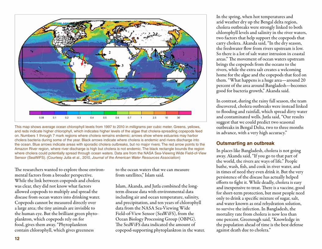
In the spring, when hot temperatures and arid weather dry up the Bengal delta region, cholera outbreaks were strongly linked to both chlorophyll levels and salinity in the river waters, two factors that help support the copepods that carry cholera. Akanda said, “In the dry season, the freshwater flow from rivers upstream is low. So there is a lot of salt water intrusion in coastal areas.” The movement of ocean waters upstream brings the copepods from the oceans to the rivers, while the extra salt creates a welcoming home for the algae and the copepods that feed on them. “What happens is a huge area—around 20 percent of the area around Bangladesh—becomes good for bacteria growth,” Akanda said.

In contrast, during the rainy fall season, the team discovered, cholera outbreaks were instead linked to flooding and rainfall, which spread dirty water and contaminated wells. Jutla said, “Our results suggest that we could predict two seasonal outbreaks in Bengal Delta, two to three months in advance, with a very high accuracy.”

Outsmarting an outbreakIn places like Bangladesh, cholera is not going away. Akanda said, “If you go to that part of the world, the rivers are ways of life.” People bathe, wash, fish, and cook in river water, and in times of need they even drink it. But the very persistence of the disease has actually helped efforts to fight it. While deadly, cholera is easy and inexpensive to treat. There is a vaccine, good for short-term protection, but most people need only to drink a specific mixture of sugar, salt, and water known as oral rehydration solution, to survive the infection. In Bangladesh, the mortality rate from cholera is now less than one percent. Greenough said, “Knowledge in the population ahead of time is the best defense against death due to cholera.”

This map shows average ocean chlorophyll levels from 1997 to 2010 in milligrams per cubic meter. Greens, yellows, and reds indicate higher chlorophyll, which indicates higher levels of the algae that cholera-spreading copepods feed on. Numbers 1 through 7 mark regions where cholera remains endemic; arrows show where estuaries may harbor cholera bacteria during some of the year. Black arrows indicate where cholera is endemic and rivers discharge into the ocean. Blue arrows indicate areas with sporadic cholera outbreaks, but no major rivers. The red arrow points to the Amazon River region, where river discharge is high but cholera is not endemic. The black rectangle bounds the region where cholera could potentially spread through ocean waters. Data are from the NASA Sea-Viewing Wide Field-of-View Sensor (SeaWiFS). (Courtesy Jutla et al., 2010, Journal of the American Water Resources Association)

0.08 0.1 0.2 0.3 0.4 0.5 0.6 0.7 1 2.5 10 30

13

But in other parts of the world, cholera appears unexpectedly and can catch vulnerable populations unprepared. In Haiti, for example, cholera appeared months after a massive earthquake reduced cities to rubble. Before that outbreak, Haiti had not seen cholera for a hundred years. The disease spread to more than 400,000 people in Haiti in the few months after it started and by March 2011, it had killed 4,600. Knowing a few months ahead of time that cholera would strike could have given aid workers enough time to intervene. Greenough said, “In areas where you identify the risk, you could get in well ahead of time and immunize the population at a very low cost and provide accurate information about making and using oral rehydration therapy solutions.”

Islam and his team are now expanding their research to other regions that see occasional cholera outbreaks, and other underdeveloped areas where a cholera outbreak can cause massive illness and death. Islam said, “We want to create actionable knowledge. We want to be able to predict what will be the next Haiti.”

To access this article online, please visit http://earthdata.nasa .gov/sensing-our-planet/2011/time-cholera

References Akanda, A. S., A. S. Jutla, M. Alam, G. C. de Magny, A. K. Siddique, R. B. Sack, A. Huq, R. R. Colwell, and S. Islam. 2011. Hydroclimatic influences on seasonal and spatial cholera transmission cycles: implications for public health intervention in the Bengal Delta. Water Resources Research. In press.Jutla, A. S., A. S. Akanda, and S. Islam. 2010. Tracking cholera in coastal regions using satellite observations.

Journal of the American Water Resources Association 46 (4):651-662, doi:10.1111/j.1752-1688.2010.00448.x.Kuehn, B. M. 2010. Use of Earth-observing satellite data helps us predict, prevent disease outbreaks. Journal of the American Medical Association 303 (5):403-405, doi:10.1001/jama.2010.32.

For more informationNASA Ocean Biology Processing Group http://oceancolor.gsfc.nasa.govSea-Viewing Wide Field-of-View Sensor (SeaWiFS) http://oceancolor.gsfc.nasa.gov/SeaWiFS/

About the remote sensing data used

Satellite GeoEye OrbView-2

Sensor Sea-Viewing Wide Field-of-View Sensor (SeaWiFS)

Data set SeaWiFS Monthly Chlorophyll Data

Resolution 9 kilometer

Parameter Chlorophyll concentration

Data center NASA Ocean Biology Processing Group (OBPG)

About the scientists

Ali Akanda is a PhD student in engineering at Tufts University, studying the impact of climate variability and change on freshwater availability, access to safe water and sanitation, and public health. The National Institutes of Health under a grant from the American Recovery and Reinvestment Act supported his research. (Photograph courtesy A. Akanda)

Dr. William Greenough is a professor of medicine and international health at Johns Hopkins University. He is an expert on cholera and other diarrheal diseases. (Photograph courtesy W. Greenough)

Shafiqul Islam is a professor of civil and environmental engineering at Tufts University, where he researches water quality issues ranging from cholera to climate change. The National Science Foundation, the National Institutes of Health, and NASA supported his research. (Photograph courtesy S. Islam)

Antarpreet Jutla is a PhD student in engineering at Tufts University. His research focuses on using remote sensing to understand and predict large scale hydroclimatological controls on outbreaks of water-related diseases. The National Institutes of Health under a grant from the American Recovery and Reinvestment Act supported his research. (Photograph courtesy A. Jutla)

14

by Jane Beitler

Flood waters were rising near the small farming village in China where ecologist Erle Ellis was staying. He scrubbed his research project and evacuated, but he would return. Ellis had been studying the ecology of the Yangtze Delta since the early 1990s, yet he was often surprised by how its people and ecology overturned his assumptions.

Neither flood nor repeated famines have managed to wipe out the people who have lived

here for thousands of years. Long ago, they reshaped the landscape to grow rice in swampy paddies in the vast plains of the Yangtze and up into the hillsides. Houses settled on the valley floor, ringed with gardens and trees. Generations farmed the still-thriving land.

It is strange to find an ecologist studying land settled by people. Historically, ecologists have studied wild places. But Ellis thinks it is time for ecologists to pay more attention to landscapes with people, and he is using Earth science data to prove the point.

Repatterning the world

“We think of our influence as being small. That’s not the way the world works anymore.”

Navin RamankuttyMcGill University

People built these terraces to grow rice, in the Cordillera Mountains, north of Manila in the Philippines. They are one example of how humans have transformed ecologies around the world. (Courtesy S. Ciencia)

15

The complete cycleThe Yangtze Delta is home to more than eighty million people in an area only a little larger than the state of Indiana. How does the land support this much agriculture and so many people, and can it continue to thrive? It is a question that continues to intrigue Ellis, and that may teach our teeming numbers to wisely manage the lands that feed us.

When he first came to China, Ellis expected to see older forms of agriculture persisting. He wanted to study small farms, and talk to farmers who still worked them by hand. He expected to be wading knee-deep in rice fields fertilized by manure. Ellis felt it would be vastly different from most farms in the United States that worked more like factories, using machinery and chemicals to grow food on a large scale. “We think of agriculture as being something out there far away with big machines,” he said. “In most of the world that is not the case.”

Chinese farms did look traditional at first glance; people worked the rice paddies by hand, sometimes using water buffalo instead of tractors. Up close, Ellis saw modern ways arising from agricultural science, such as the heavy use of chemical fertilizers. “Today about a third of the world’s fertilizer is used in China—but almost all of that is applied by hand,” he said. In spite of some residue of older practices, Ellis thinks that traditional systems, which rely on local knowledge and natural resources, are almost completely gone.

Like other nations around the world, China is using technologies like fertilizer and pesticides to boost production and feed its population. “It is quite a rare thing now to have a highly produc-tive traditional agriculture, because there is not

much desirable about it,” Ellis said. “Famines were common.” Before the 1970s, Chinese scholars over a thousand years recorded large numbers of famines every year across the country. Although crop failures and food shortages are not the only factors in famine, growing and storing a surplus of food can help avert famine. The high nitrogen content in chemical fertilizers can double and triple crops, compared to fertilizers like manure. “In China that is not a trivial thing,” he said. “If you cut their yields in half, without massive imports, people would starve.”

Ironically, while other countries are taking up industrial-style farming, many in the United States are calling for more local and organic farming, thinking that it is more environmentally friendly. Chemical fertilizer can pollute groundwater and surface water, especially when it reaches coastal waters. Too much nitrogen in soils can even reduce plant growth. Heavy doses of fertilizer added to the soil can break down and wind up as more nitrogen in the atmosphere. Nitrogen oxides, which are ozone-depleting chemicals and greenhouse gases, contribute to global warming, along with carbon emissions from heavy machinery and long-distance transportation of food. “Humans have doubled the amount of reactive nitrogen in the nitrogen cycle globally,” Ellis said.

So small changes in little villages, added together, can matter in a big way. But few ecologists seemed to be studying places that people live.

I produce, therefore I amAfter his years in China, Ellis thought the land-scapes people use, and their large-scale impacts, were poorly understood. Part of the reason was how ecologists viewed the Earth. “If you open atlases or global change textbooks, you see maps

of biomes of the world. This is how you depict what the world looks like,” said Navin Ramakutty, at McGill University.

Ecologists use biomes to classify the global patterns of ecology on land, based on vegetation types that correspond to global patterns in climate. The different biomes—lush tropical forests, hot arid deserts, grasslands, or cold, arid tundra—can each support unique kinds and amounts of life. They also make different contributions to the global carbon cycle.

Like other modern sciences, ecology strives for objectivity by reducing the complexity of the systems they study. One way to do this has traditionally been to isolate human influence from observations, by studying areas presumed to be wild. The lands that we influence, such as croplands and cities, tend to be excluded from consideration, or squeezed into just a few land classifications, where they were largely ignored by ecologists until recently.

A rural man poses with his donkey near Ziz, Morocco. This area is representative of the Populated Rangelands anthrome: low population, few crops, and flat lands used mainly for livestock grazing. (Courtesy E. Ellis)

16

But almost seven billion people live on Earth today. “We know instinctively that this is not what the world looks like any more,” Ramankutty said. Ramankutty and Ellis are among a growing number of ecologists who think the classic focus on wildlands does not match the state of the Earth today.

Ellis noted, “What is the ecology that people create and sustain over a long period of time? In the past, this was a very marginal subject for

ecologists. If you have people in your ecosystem it’s not really ecology. It’s a degraded thing, an unimportant ruined thing. For me that was always very frustrating.”

People in the mapEllis thought that data could show how much of the Earth is under human influence. “I wanted to quantify and express in a powerful way to ecologists the significance of anthropogenic ecosystems,” he said.

He proposed to Ramankutty, who had been using global data to study patterns of land use for agriculture, that they look at population and land use statistics. Ramankutty said, “The sheer number of people affects ecosystem processes in the village landscapes that Erle had been studying. He thought of extending this idea to a global scale.”

As they melded global data sets on population, land use, and land cover, patterns emerged. Ellis said, “There was no obvious method for determining the big categories of the anthrome system, so we did a statistical approach that figured out the global patterns in these data.” The researchers saw a new biome system, with human-dominated ecosystems that they called anthropogenic biomes, or anthromes for short.

The analysis produced two major insights. Ramankutty said, “First, an astonishing amount of the world’s landscape, up to 77 percent, is an anthrome.” People have taken over most places on Earth that can support human life. Some wildlands remain in rainforests, but most are in cold, arid, northern areas. “Second, we usually think of people living in cities between forests, or between forests practicing agriculture,” Ramankutty said. “We think of our influence as being small. That’s not the way the world works anymore. We currently have human systems within which natural systems are embedded.”

The data also showed more human-influenced categories than just the classic cropland or urban area biomes. Ellis said, “There’s this incredible richness of systems and ecosystems that we create and sustain. For example, in the temperate zone you see trees. Just about every system, urban or agricultural, has trees. We create mosaics; we hardly ever create one thing. When you look at

This map classifies the Earth’s land area into categories of ecosystems created by humans based on population, land use, and vegetation. The lightest green and gray areas represent the world’s remaining wildlands, mostly in boreal and tropical forests and cold, dry northern regions. Wildlands account for less than 23 percent of Earth’s land surface. (Courtesy E. Ellis and N. Ramankutty/NASA Earth Observatory/SEDAC)

SettlementsUrbanDense SettlementsRice VillagesIrrigated VillagesCropland & PastoralPastoral VillagesRainfed VillagesRainfed Mosaic Villages

CroplandsResidential Irrigated CroplandResidential Rainfed MosaicPopulated Irrigated CroplandPopulated Rainfed CroplandRemote Croplands

RangelandsResidential RangelandsPopulated RangelandsRemote Rangelands

ForestedRemote ForestPopulated Forest

WildlandsBarren or Ice-coveredSparse TreesWild Forest

17

the Earth from space—when you look out of the airplane—you can see it.”

The ecologies of these mosaics were a question mark for researchers. Ramankutty said, “We think that you can have valuable ecosystems in places where humans live. There can be valuable carbon stored in trees in urban landscapes. There are more trees in cropland anthromes than in wildland anthromes. We should measure those things as well.”

A new eraThe result of their analysis is now published as a data set at the NASA Socioeconomic Data and Applications Center (SEDAC). Users can obtain mapped data on anthropogenic biomes, for the globe or for one or more of six regions. In all, the analysis defines twenty-one classifications of biomes; only three are wild.

The researchers think the data and the new classifications show that the field of ecology can no longer ignore human influence. While classic biome systems are by no means obsolete, Ramankutty said, “We shouldn’t always be jaunting off to the middle of the rainforests to study how ecosystems work. We should be studying ecosystems in places where people live and manage land.”

To know that humans dominate Earth can be unsettling. Ellis said, “The way we value nature is challenged in some way by the idea that most of the planet has been transformed into human systems already.” Humans need to understand and manage the lands they use and live in, now and for the future.

Ramankutty added, “You start by talking about the negative—that humans are really in control

of ecosystems around the planet. Compared to other species we have been extremely successful, and we have had an impact on a global scale.”

“But the positive thing is, that same story tells us humans are extremely capable. If we set our minds to it, we should be able to find new solutions to continue to flourish on this planet.”

To access this article online, please visit http://earthdata.nasa .gov/sensing-our-planet/2011/repatterning-world

ReferenceEllis, E. C. and N. Ramankutty. 2008. Putting people in the map: anthropogenic biomes of the world. Frontiers in Ecology and the Environment 6(8): 439-447.

For more informationNASA Socioeconomic Data and Applications Center (SEDAC) http://sedac.ciesin.columbia.eduEnvironmental Sustainability—Anthropogenic Biomes Version 1 http://sedac.ciesin.columbia.edu/es/ anthropogenicbiomes.htmlLaboratory for Anthropogenic Landscape Ecology http://ecotope.org

About the data used

Satellite Terra

Sensor Moderate Resolution Imaging Spectroradiometer (MODIS)

Data sets Anthropogenic Biomes Version 1 MODIS Land Cover Type

Resolution Raster cell sizes are 5” or 0.08333 degree decimal (about 10 kilometers at the equator)

15 arc second

Parameters Anthropogenic biomes Land cover

Data centers NASA Socioeconomic Data and Applications Center (SEDAC)

NASA Land Processes Distributed Active Archive Center (LP DAAC)

About the scientists

Erle Ellis is an associate professor of geography and environmental systems at the University of Maryland, Baltimore County. His research investigates the ecology of anthropogenic landscapes and their changes at local and global scales. (Photograph courtesy E. Ellis)

Navin Ramankutty is an assistant professor in the Department of Geography and Earth System Science Program at McGill University, Montreal, Canada. He co-directs the Land Use and the Global Envi-ronment research program, which uses Earth observations and analysis to understand how changes in the land and climate change modify global ecosystem structure and human well-being. (Photograph courtesy McGill University)

18

by Katherine Leitzell

Even on a good day, the Egyptian capital and its neighboring Nile Delta cities suffer from some of the worst air pollution on Earth. Two million cars prowl the traffic-clogged streets, while a thousand factories belch smoke into the air. On top of the everyday pollution, farmers outside the city burn leftover rice husks at the end of the growing season, adding smoke to already smoggy air.

On a bad day, the smog in the city is unbearable. And those bad days now happen like clockwork, appearing every fall since 1999 and lasting days at a time. As the summer heat fades, a so-called “black cloud” settles over the city, smothering the Nile Delta in a black-brown haze that burns people’s eyes and throats.

How can Egyptians get rid of the black cloud? The first problem was, as Heba Marey, a scientist

A black cloud over Cairo

The city of Cairo is barely visible behind the pyramids in this photograph, due to the heavy layer of haze. (Courtesy P. Medved)

“Cairo’s air has become overloaded.”

Heba MareyUniversity of Alexandria

19

at the University of Alexandria in Egypt, said, “Researchers didn’t have a firm cause for the black cloud formation.” In 2009, as a doctoral student studying remote sensing, Marey realized that sat-ellite data might lead to a clear answer that would be key to reducing the pollution at its source.

Worst pollution on the planetIn 2007 the World Bank ranked Cairo’s air worst in the world for pollution by particulates, the tiny fragments of soot or dust that are most damaging to human lungs. High emissions contribute to the problem, but Cairo’s topography and climate make the pollution even worse. The city lies in a valley surrounded by hills, which hold the poisoned air like water in a bowl. In the fall, frequent temperature inversions settle over Cairo—a weather phenomenon that occurs when a warmer, lighter air mass moves over a colder, denser air mass, trapping a layer of air close to the ground. The inversions still the winds, creat-ing a stagnant soup of unmoving air. Meanwhile, an extremely dry climate means that cleansing rainstorms rarely appear.

But the black cloud is different from the pollu-tion that plagues the city every day. It appears only once a year, in September or October. And it is much more intense than the regular pollution, darkening the sky into a foreboding smog. The black cloud brings pollution levels up to ten times the limits set by the World Health Organization, and can persist for days or weeks at a time. It sends people to the hospital with exacerbated lung infections and asthma attacks at unusually high rates, and contributes to cancer and other long-term health problems.

Before Marey started her research, the source of the pollution cloud was a mystery. People in the

city blamed farmers’ fires, while many farmers, who live a hundred miles outside Cairo, argued that their smoke could not feasibly travel all the way to Cairo, and that the cause must instead be the cars and factories in the city itself. In 2004, authorities banned rice husk burning and intro-duced other pollution-reducing measures, but the annual cloud continued.

Marey wanted to look at the problem from a different perspective. Even though people had guesses about the reasons for the black clouds, the ground data available in Egypt only gave people the same information that they could already see with their own eyes: air pollution got much worse during the black cloud events.

Marey had received a research fellowship to study abroad as part of her PhD work, and decided to use it to learn more about the black cloud. She contacted John Gille at the National Center for Atmospheric Research (NCAR) in Colorado and proposed that they work together. “NCAR is the best place in the world for atmospheric remote sensing science,” Marey said. “It was a wonderful opportunity to work there.”

When she arrived in Colorado, Gille helped Marey learn more about remote sensing and explore the available data. Then she moved on to put the pieces together for her study. Gille said, “She was very enterprising. She talked to a lot of people, asked a lot of questions, and found the data sets she needed to answer her questions.”

New view of pollutionMarey started by looking at the agricultural fires that burned outside Cairo each fall, using NASA Moderate Resolution Imaging Spectroradiometer (MODIS) fire count maps, which showed the

locations and intensity of fires. The data showed that fires were closely linked in time with the pol-lution, preceding the black cloud’s arrival by just six to nine hours.

The timing of the fires was a strong clue, but it did not prove that the smoke from the fires reached Cairo. To trace the path of the smoke plumes, Marey used Multi-Angle Imaging Spec-troradiometer (MISR) data from the NASA Langley Research Center Atmospheric Science Data Center. Using a tool called the MISR Interactive Explorer (MINX), and trajectory analysis models, she combined the plume data with the fire data and atmospheric models to

This image from the Multi-Angle Imaging Spectroradi-ometer (MISR) instrument, on board the NASA Terra satellite, helped researchers trace the source of a heavy smoke plume over Cairo, Egypt. The colored spots indicate plume height measurements, with abundant bright blue-green spots showing that the smoke mostly resided in the lower 500 meters (1,600 feet) of the at-mosphere. The arrow pointing south shows the direction that the plumes were drifting. (Courtesy H. Marey et al.)

0 1,000Height (m)

20

learn where the smoke plumes originated, and where they traveled. As it turned out, the plumes blew directly towards Cairo.

Those two findings showed that smoke plumes were contributing to the black cloud. But it did not explain why the pollution was so persistent. Using temperature, meteorological data, and models that described the movement of smoke and pollution, Marey found an explanation. After rice husk burning was made illegal, farmers started burning it at night and early in the morning, when they are less likely to get caught. The fires now burn at the worst possible time for Cairo’s air. “The pollution reaches Cairo after sunset, which is just when the temperature inversion starts to form,” she said. Marey also found that the black cloud lurks low to the ground, concentrated in the bottom 500 meters (1,600 feet) of the atmosphere. Since the pollu-tion hangs low as it travels, it slides into the city close to the ground, where it can be trapped by the temperature inversion.

All the clues pointed to agricultural fires as the source of the black cloud. But if that was true, why did the black cloud not appear before 1999? Marey only had satellite data back to 2000, so she could not use it to look at the differences between the decades. Instead, she turned to agricultural statistics, which showed a sharp growth in rice production between 1990 and 2000. Rice production increased from about three million tons in 1990 to nearly six million tons in 2000. As rice production grew, farmers had more tons of rice husks to burn. At the same time, farmers were upgrading their homes to cook with gas stoves rather than burning rice husks for fuel, which meant they had more leftover plant material to get rid of all at once.

This aerial photograph shows an agricultural field burning in the Nile Valley. Burning helps prepare fields for the next crop, but some kinds of agricultural burning have been prohibited to help curb air pollution in the Cairo area. (Courtesy I. Duffy)

21

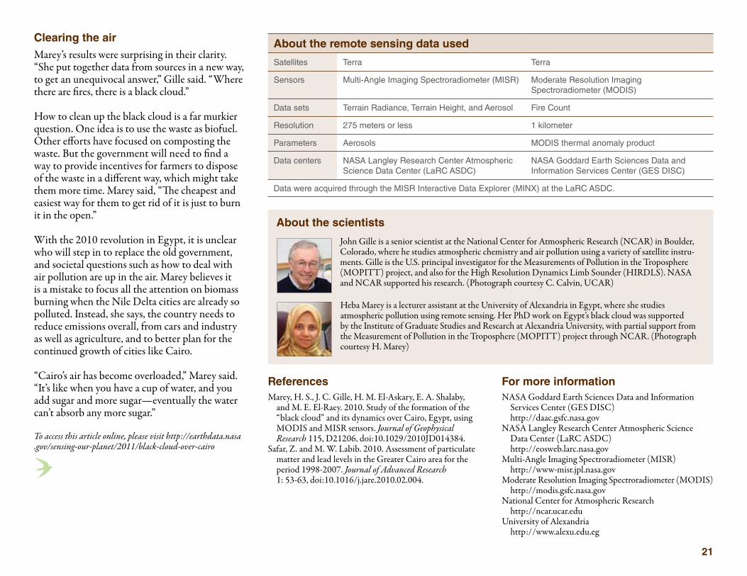
Clearing the airMarey’s results were surprising in their clarity. “She put together data from sources in a new way, to get an unequivocal answer,” Gille said. “Where there are fires, there is a black cloud.”

How to clean up the black cloud is a far murkier question. One idea is to use the waste as biofuel. Other efforts have focused on composting the waste. But the government will need to find a way to provide incentives for farmers to dispose of the waste in a different way, which might take them more time. Marey said, “The cheapest and easiest way for them to get rid of it is just to burn it in the open.” With the 2010 revolution in Egypt, it is unclear who will step in to replace the old government, and societal questions such as how to deal with air pollution are up in the air. Marey believes it is a mistake to focus all the attention on biomass burning when the Nile Delta cities are already so polluted. Instead, she says, the country needs to reduce emissions overall, from cars and industry as well as agriculture, and to better plan for the continued growth of cities like Cairo.

“Cairo’s air has become overloaded,” Marey said. “It’s like when you have a cup of water, and you add sugar and more sugar—eventually the water can’t absorb any more sugar.”

To access this article online, please visit http://earthdata.nasa .gov/sensing-our-planet/2011/black-cloud-over-cairo

References Marey, H. S., J. C. Gille, H. M. El-Askary, E. A. Shalaby, and M. E. El-Raey. 2010. Study of the formation of the “black cloud” and its dynamics over Cairo, Egypt, using MODIS and MISR sensors. Journal of Geophysical Research 115, D21206, doi:10.1029/2010JD014384.Safar, Z. and M. W. Labib. 2010. Assessment of particulate matter and lead levels in the Greater Cairo area for the period 1998-2007. Journal of Advanced Research 1: 53-63, doi:10.1016/j.jare.2010.02.004.

For more informationNASA Goddard Earth Sciences Data and Information Services Center (GES DISC) http://daac.gsfc.nasa.govNASA Langley Research Center Atmospheric Science Data Center (LaRC ASDC) http://eosweb.larc.nasa.govMulti-Angle Imaging Spectroradiometer (MISR) http://www-misr.jpl.nasa.govModerate Resolution Imaging Spectroradiometer (MODIS) http://modis.gsfc.nasa.govNational Center for Atmospheric Research http://ncar.ucar.eduUniversity of Alexandria http://www.alexu.edu.eg

About the scientists

John Gille is a senior scientist at the National Center for Atmospheric Research (NCAR) in Boulder, Colorado, where he studies atmospheric chemistry and air pollution using a variety of satellite instru-ments. Gille is the U.S. principal investigator for the Measurements of Pollution in the Troposphere (MOPITT) project, and also for the High Resolution Dynamics Limb Sounder (HIRDLS). NASA and NCAR supported his research. (Photograph courtesy C. Calvin, UCAR)

Heba Marey is a lecturer assistant at the University of Alexandria in Egypt, where she studies atmospheric pollution using remote sensing. Her PhD work on Egypt’s black cloud was supported by the Institute of Graduate Studies and Research at Alexandria University, with partial support from the Measurement of Pollution in the Troposphere (MOPITT) project through NCAR. (Photograph courtesy H. Marey)

About the remote sensing data used

Satellites Terra Terra

Sensors Multi-Angle Imaging Spectroradiometer (MISR) Moderate Resolution Imaging Spectroradiometer (MODIS)

Data sets Terrain Radiance, Terrain Height, and Aerosol Fire Count

Resolution 275 meters or less 1 kilometer

Parameters Aerosols MODIS thermal anomaly product

Data centers NASA Langley Research Center Atmospheric Science Data Center (LaRC ASDC)

NASA Goddard Earth Sciences Data and Information Services Center (GES DISC)

Data were acquired through the MISR Interactive Data Explorer (MINX) at the LaRC ASDC.

22

by Jane Beitler

Six hundred and fifty thousand years ago, mam-moths and mastadons cavorted on the plains of North America, on the fringes of a massive sheet of ice almost two miles thick in places and as big

as a continent, covering most of what are now Canada and the upper United States.

Earth warmed, and the ice sheets receded, so people can now live in places once buried by ice like Quebec and Chicago. Correctly speaking,

The un-ice age

The Advanced Spaceborne Thermal Emission and Reflection Radiometer (ASTER) on the NASA Terra satellite acquired this image of Umiamiko Glacier in Greenland. Researchers have observed rapid melt of the Greenland Ice Sheet and its glaciers in recent years, adding water to the world’s oceans. (Courtesy J. Box and I. Howat/ASTER)

“When we saw the trend, it was a bad surprise.”

Ted ScambosNational Snow and Ice Data Center

23

Earth remains in an ice age. Ice still sits thick atop Greenland and Antarctica, holding enough water to raise sea levels by hundreds of feet; and in recent decades, the ice sheets have begun to melt more rapidly.

Is global warming pushing Earth into an ice-free age? Scientists doubt a total melt this century, but think there could be enough to raise sea levels up to three feet. Only a foot or two could drive millions of coastal dwellers to higher ground. A closer estimate of the potential for sea level rise from ice sheet melting would give low-lying communities around the world more time to figure out how to adapt.

Icing up

Water on Earth resides in liquid form in the ocean, lakes, rivers, and underground, in mois-ture form in the air and soil, and in solid form as ice and snow. The total amount of water on Earth is more or less constant. Water can redis-tribute within the Earth; the water contained in the massive ice sheets on land during the ice ages originated from the oceans. As a result, at the peak of the ice ages, sea levels were 400 feet lower than they are today.

Today Earth is in an interglacial period, a relatively warmer period of the current ice age, but in recent decades Earth’s climate has been warming. While past shifts took hundreds or thousands of years, today people may be able to see changes in their lifetimes. Only a few degrees of cooling or warming can alter the balance between ice age and ice melting, and the begin-nings of that melt are evident. Ted Scambos, a glaciologist at the National Snow and Ice Data Center said, “Greenland mass loss started in the most likely place—at the southern glacier

outlets—then spread to the rest of the island. In Antarctica, it started at the northernmost point on the Antarctic Peninsula, and on the coast of the West Antarctic Ice Sheet, at Pine Island Bay.”

Isabella Velicogna, an assistant professor at the University of California Irvine, said, “It’s hard to make long-term predictions, but we see that things are changing fast.” The questions pile up like the ice once did: How fast is it melting? How much will sea levels rise, and when? What will this mean to people along low-lying coasts? Melting downWhat scientists know about how these ice sheets grow and shrink has been hard won. They have dragged sled-mounted radars across the vast Antarctic continent to probe its ice cover. They planted gauges on glaciers to monitor their shedding of ice towards the sea. They camped on Greenland’s ice sheet to watch melt water pour down deep drain holes that pock the ice

sheet in summer. They combed satellite imagery for changes to the outlines of the ice sheets, and saw the sudden collapses of ice shelves that fringe Antarctica’s edges. In recent decades, they have witnessed telltale signs of warming unlike any in the last thousand or more years.

But putting absolute numbers on the cubic feet of ice on land, and the melt water flowing into the oceans, is a slippery problem. It meant figuring the amount of ice being added as snow-fall, and subtracting ice and melt water flowing into to the ocean. Scambos said, “We didn’t have enough measurements of snow accumulation in Antarctica, so when earlier models estimated the mass input to the ice sheet, they could be slightly off in the middle of the ice sheet. That can add up to a lot over a huge area.”

Glaciers on Greenland and Antarctica have also changed rapidly in recent decades. Large shelves of ice floating on the ocean in front of outlet

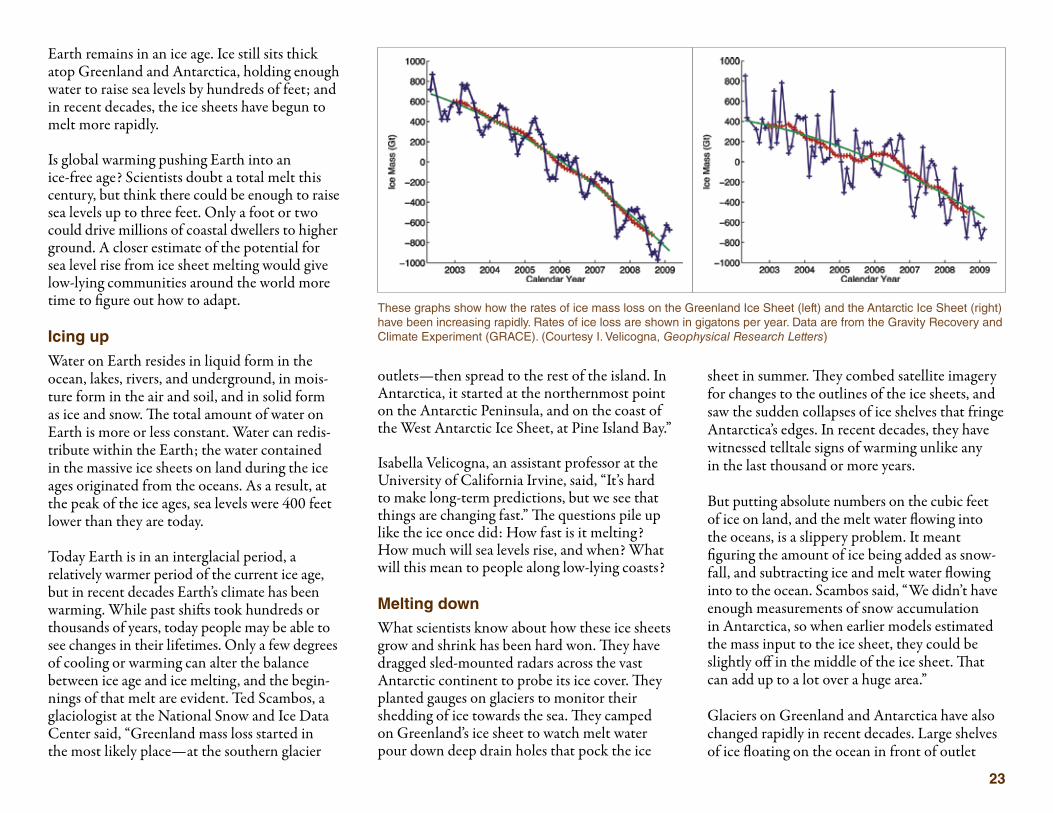
These graphs show how the rates of ice mass loss on the Greenland Ice Sheet (left) and the Antarctic Ice Sheet (right) have been increasing rapidly. Rates of ice loss are shown in gigatons per year. Data are from the Gravity Recovery and Climate Experiment (GRACE). (Courtesy I. Velicogna, Geophysical Research Letters)

24

valleys, where glaciers shed their ice into the ocean, help slow glaciers down. The warming of recent decades has resulted in the break up and rapid collapse of several ice shelves. “When the glaciers were suddenly freed from the gate, they began galloping along,” Scambos said.

New information came from the NASA Ice, Cloud, and Land Elevation Satellite (ICESat), which used a laser to measure the height of the ice sheet. Launched in 2003, it was providing a clearer picture of ice thickness when it ceased operations in 2010. NASA filled in with a series of missions with sensors flown on aircraft, called IceBridge, and has planned a second ICESat

mission in 2015. “IceBridge is giving us a cross section of glaciers, a gallery of detailed descrip-tions,” Scambos said. But the big picture is still elusive, and the ice sheets are not waiting.

A quicker pictureSeeking more data on the changes, Velicogna and others turned to a very different source. “The GRACE [Gravity Recovery and Climate Experiment] satellites weigh the Earth every thirty days and look at how the mass is chang-ing,” Velicogna said. “We can see many things, like water storage on land, and how much ice is stored on the ice sheets. You can see the changes in mass month to month.”

GRACE, a joint mission of NASA and the German Space Agency, does not actually weigh the Earth; it measures Earth’s gravity. Gravity varies with changes in mass: it varies slightly with latitude and elevation, and with geology, like denser rocks or mountains. The twin GRACE satellites orbit in tandem, measuring micro-meters of change in the distance between them, caused by small deviations in gravity.

Changes in the location of water or ice on the Earth surface also cause gravity variations. GRACE picks up the gravity signal of the ice sheets, and scientists can measure how the signal changes as the sheets change. In 2009, Velicogna isolated the gravity data for Greenland and Antarctica, turning the data into mass change measurements. She compared mass from month to month and year to year since the satellites launched in 2002. Now she had data on how it changed—and mass change could be converted directly into water volume.

Though scientists suspected that the ice sheets were losing ground, the rate surprised them. According to the GRACE data, Greenland had been losing mass at a rate of 137 billion tons, or gigatons, per year, during 2002 to 2003. (A gigaton equals the weight of about 142 million African elephants.) By 2007 to 2009, the loss had accelerated to 286 gigatons per year. More startling was that Antarctica’s mass loss also sped up dramatically, from 104 gigatons per year to 246 gigatons per year.

The GRACE data may help the rate of scientists’ understanding match the accelerating rate of ice sheet change. Velicogna said, “We really need a longer record. We have made incredible improve-ments over the last decade in our understanding

Researchers camp on the Antarctic Ice Sheet, preparing to set up instruments to measure the state of the glaciers that flow into what is left of the Larsen B Ice Shelf. A large portion of the Larsen B collapsed dramatically in 2002; immediately afterwards, glaciers were observed to accelerate their flow of ice into the ocean. (Courtesy T. Scambos)

25

As summer sunshine and warmth melt the surface of the Greenland Ice Sheet, melt water pours into large, deep holes in the ice, called moulins. (Courtesy K. Steffen, CIRES/University of Colorado Boulder)

26

of Antarctic mass balance. Before GRACE, we thought that Antarctica would gain mass.” Warmer air temperatures cause more snow to fall on the interior of Antarctica, helping it gain mass. Scambos said, “Isabella’s study using the GRACE data, and other studies, show that increased snowfall is not enough to offset the loss at the coasts.”

Scientists are still working to zero in on the rate of change likely over coming decades. However jagged the line of descent may be, it is pointed

downward. Scambos said, “When her study came out, and we saw the trend, it was a bad surprise. It will not go down this road slowly—it will pick up speed. It is not going away.”

Future coastlinesHow sea level rise will change our coasts is no straight-line problem either. The ocean is not like a flat pan of water that rises equally when water is added. Velicogna said, “If you take a boat and sail the ocean, take your GPS and measure elevation, you see that the ocean is not flat. Gravitational

pull shapes the sea surface. If you put more water in the ocean, it will go to the lowest point. So in some places, sea level will rise more than others. In addition there are waves and tides.” Millions of people around the world live in low-lying deltas that scientists think will be under water in coming decades.

“We have to think about what we can do to miti-gate the changes,” Velicogna said. “It is not going to happen today or tomorrow, but eventually. If we are a rich country we can build a different

This aerial photograph of the Antarctic coast shows Punchbowl Glacier. Both Antarctic glaciers and the Antarctic Ice Sheet contain large amounts of fresh water, which could be added to the world’s oceans as climate warms. (Courtesy T. Scambos and R. Bauer)

27

house, but it has a cost. There are places such as Bangladesh that are not so rich.”

Even better-off economies will change, as people move from low-lying areas to higher ground. “It takes time to adapt,” she said. “People in places like the Netherlands that are already below sea level are more concerned than people in the U.S.”

While the future can be troubling to think about, scientists like Scambos and Velicogna are optimistic that scientific knowledge will help us adapt to a new age with smaller ice sheets and bigger oceans. Velicogna said, “It’s a great field to be in, that’s what I say to the students. It’s great that we have all these satellite data. There is a lot we can learn.”

To access this article online, please visit http://earthdata.nasa .gov/sensing-our-planet/2011/un-ice-age

References Climate change past and future: The Ice Ages. http://earthguide.ucsd.edu/virtualmuseum/ climatechange2/01_1.shtmlKhan, S. A., J. Wahr, M. Bevis, I. Velicogna, and E. Kendrick. 2010. Spread of ice mass loss into northwest Greenland observed by GRACE and GPS. Geophysical Research Letters 37, L06501, doi:10.1029/2010gl042460. Scambos, T. A., J. Bohlander, C. Shuman, and P. Skvarca. 2004. Glacier acceleration and thinning after ice shelf collapse in the Larsen B embayment, Antarctica. Geophysical Research Letters 31, doi:10.1029/2004GL020670.Velicogna, I. 2009. Increasing rates of ice mass loss from the Greenland and Antarctic ice sheets revealed by GRACE. Geophysical Research Letters 36, L19503, doi:10.1029/2009GL040222.

For more informationNASA Physical Oceanography Distributed Active Archive Center (PO.DAAC) http://podaac.jpl.nasa.govGRACE Tellus Gravity Recovery and Climate Experiment http://grace.jpl.nasa.gov Isabella Velicogna http://www.faculty.uci.edu/profile.cfm?faculty_ id=5518Ted Scambos http://nsidc.org/research/bios/scambos.htmlQuick Facts on Ice Sheets http://nsidc.org/quickfacts/icesheets.html

About the remote sensing data used

Satellite Gravity Recovery and Climate Experiment (GRACE)

Sensor K-Band Ranging System

Data set GRACE Level 2 Products

Resolution 1 degree

Parameter Gravity fields

Data center NASA Physical Oceanography Distributed Active Archive Center (PO.DAAC)

This study used GRACE gravity field solutions generated at the Center for Space Research at the University of Texas (http://www.csr.utexas.edu/grace).

About the scientists

Ted Scambos is a glaciologist at the National Snow and Ice Data Center, at the University of Colorado Boulder. His research interests include remote sensing of the poles, climate change effects on the cryosphere, Antarctic history, geochemistry, and planetary science. NASA and the National Science Foundation supported his research. (Photograph courtesy P. Gibbons)

Isabella Velicogna is an assistant professor of Earth systems science at the University of California Irvine and a senior scientist at NASA’s Jet Propulsion Laboratory. Her research interests center on space-based climate measurements, with particular attention to cryospheric and high latitude regional studies. NASA and the National Science Foundation supported her research. (Photograph courtesy University of California Irvine)

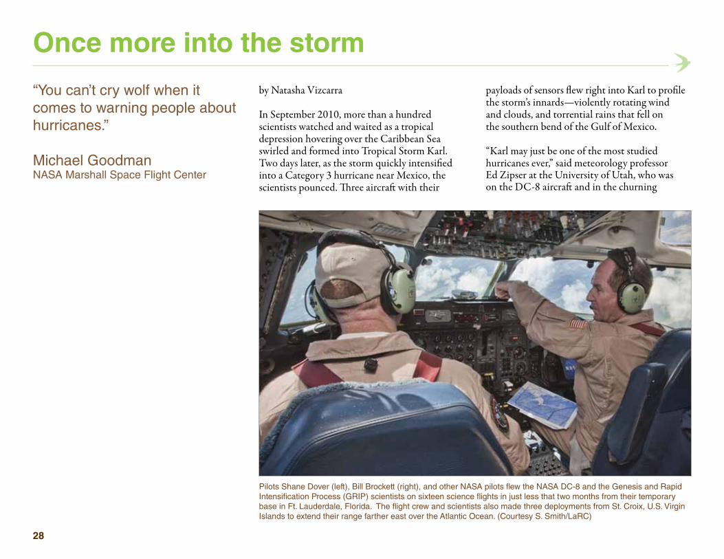
28

by Natasha Vizcarra

In September 2010, more than a hundred scientists watched and waited as a tropical depression hovering over the Caribbean Sea swirled and formed into Tropical Storm Karl. Two days later, as the storm quickly intensified into a Category 3 hurricane near Mexico, the scientists pounced. Three aircraft with their

payloads of sensors flew right into Karl to profile the storm’s innards—violently rotating wind and clouds, and torrential rains that fell on the southern bend of the Gulf of Mexico.

“Karl may just be one of the most studied hurricanes ever,” said meteorology professor Ed Zipser at the University of Utah, who was on the DC-8 aircraft and in the churning

Once more into the storm

Pilots Shane Dover (left), Bill Brockett (right), and other NASA pilots flew the NASA DC-8 and the Genesis and Rapid Intensification Process (GRIP) scientists on sixteen science flights in just less that two months from their temporary base in Ft. Lauderdale, Florida. The flight crew and scientists also made three deployments from St. Croix, U.S. Virgin Islands to extend their range farther east over the Atlantic Ocean. (Courtesy S. Smith/LaRC)

“You can’t cry wolf when it comes to warning people about hurricanes.”

Michael GoodmanNASA Marshall Space Flight Center

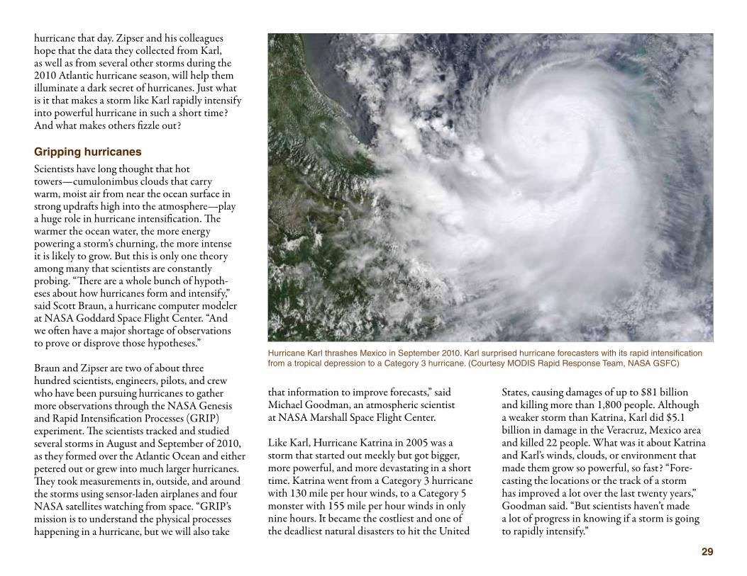
29

hurricane that day. Zipser and his colleagues hope that the data they collected from Karl, as well as from several other storms during the 2010 Atlantic hurricane season, will help them illuminate a dark secret of hurricanes. Just what is it that makes a storm like Karl rapidly intensify into powerful hurricane in such a short time? And what makes others fizzle out?

Gripping hurricanesScientists have long thought that hot towers—cumulonimbus clouds that carry warm, moist air from near the ocean surface in strong updrafts high into the atmosphere—play a huge role in hurricane intensification. The warmer the ocean water, the more energy powering a storm’s churning, the more intense it is likely to grow. But this is only one theory among many that scientists are constantly probing. “There are a whole bunch of hypoth- eses about how hurricanes form and intensify,” said Scott Braun, a hurricane computer modeler at NASA Goddard Space Flight Center. “And we often have a major shortage of observations to prove or disprove those hypotheses.”

Braun and Zipser are two of about three hundred scientists, engineers, pilots, and crew who have been pursuing hurricanes to gather more observations through the NASA Genesis and Rapid Intensification Processes (GRIP) experiment. The scientists tracked and studied several storms in August and September of 2010, as they formed over the Atlantic Ocean and either petered out or grew into much larger hurricanes. They took measurements in, outside, and around the storms using sensor-laden airplanes and four NASA satellites watching from space. “GRIP’s mission is to understand the physical processes happening in a hurricane, but we will also take

that information to improve forecasts,” said Michael Goodman, an atmospheric scientist at NASA Marshall Space Flight Center.

Like Karl, Hurricane Katrina in 2005 was a storm that started out meekly but got bigger, more powerful, and more devastating in a short time. Katrina went from a Category 3 hurricane with 130 mile per hour winds, to a Category 5 monster with 155 mile per hour winds in only nine hours. It became the costliest and one of the deadliest natural disasters to hit the United

States, causing damages of up to $81 billion and killing more than 1,800 people. Although a weaker storm than Katrina, Karl did $5.1 billion in damage in the Veracruz, Mexico area and killed 22 people. What was it about Katrina and Karl’s winds, clouds, or environment that made them grow so powerful, so fast? “Fore-casting the locations or the track of a storm has improved a lot over the last twenty years,” Goodman said. “But scientists haven’t made a lot of progress in knowing if a storm is going to rapidly intensify.”

Hurricane Karl thrashes Mexico in September 2010. Karl surprised hurricane forecasters with its rapid intensification from a tropical depression to a Category 3 hurricane. (Courtesy MODIS Rapid Response Team, NASA GSFC)

30

Small and chaoticAs it turns out, forecasting a storm’s intensity is a trickier problem to solve. “A storm’s track is an easier problem to figure out,” Braun said. Storms are steered around by the surrounding winds, which in turn are governed by the pattern of trade winds that push the ocean around in the tropics. “Large-scale processes like the trade winds evolve more slowly which makes them, in some ways, more predictable,” Braun said. “To the extent that we are able to observe the large scale winds, we can forecast track pretty readily.”

In contrast, a storm’s intensity can be influenced by everything, from the individual small cloud all the way up to massive cloud systems. “An individual cloud has the lifetime of maybe thirty minutes to an hour, whereas large-scale events are on the order of twelve to twenty-four hours,” Braun said. “Smaller processes are just so much more chaotic and harder to predict. They are also much less understood by scientists.”

To predict a storm’s intensity, researchers rely on forecast models, as they do in predicting a storm’s track. The model is made of math-ematical equations that represent a storm’s elements—like wind speed, temperature, air pressure, humidity—and what is already known about how these elements interact with each other. “The forecast model is only as good as the equations you can create to express how nature works, in addition to the information you give it on the actual state of the atmosphere,” Braun said.

Looking for strangeGRIP scientists want to plug more detailed hurricane observations into their models to improve their forecasts. So they measured as many parts of the hurricane as they could, from the tiny air particles whipped around by the winds, to its enormous cumulonimbus clouds. “By having multiple aircraft with the right array of sensors, we measured several different aspects of the storm simultaneously,” Braun said. “We

measured characteristics of the large-scale environment better, but we also measured the evolution of these smaller cloud systems, how they evolved into bigger cloud systems, and hopefully how they were interacting with the environment.” In addition to three aircraft loaded with updated and new instruments, the NASA Terra, Aqua, CloudSat, and Tropical Rainfall Measuring Mission (TRMM) satellites captured the hurricanes’ clouds and rainfall, as well as environmental conditions from space.

Nine months after the field mission and in the midst of processing the large amount of data they collected, the scientists are seeing glimmers of surprising observations that challenge what they thought they already knew about hurri-canes. Although still raw and very preliminary, the data are prompting the GRIP scientists to ask new questions. “You don’t often go into the field and come off the airplane and have ‘Eureka!’ moments,” Zipser said. “The most exciting developments in science may happen after you say, ‘Hey, that’s strange.’”

Challenging hot towersOne of the strange things that Zipser and his colleagues observed in the field and in some of the data is that tall hot towers did not seem to play as big a role in hurricane formation and intensification as they expected. “The conventional wisdom for many years is that you need these intense hot towers for genesis and for rapid intensification,” Zipser said. “Although that still may be true, we are starting to see some evidence that maybe that is not necessary.” Instead, the researchers think that less intense storm clouds may be enough. “Maybe it’s sufficient to have gentle rising towers, as long as the clouds produce a lot of rain, spread fairly

The NASA CloudSat satellite captured a slice of Hurricane Karl’s clouds at 8:01 a.m. GMT (4:01 a.m. EDT) on September 17, 2010. CloudSat shows that the clouds are over eight miles high. The blue areas along the top of the clouds indicate cloud ice. The highest clouds in Karl at the time of the image were as cold as -40 to -60 degrees Celsius (-40 to -76 degrees Fahrenheit). (Courtesy NASA/JPL/Colorado State University/NRL)

Low HighReflectivity

31

evenly around the developing storm center,” Zipser said. “That’s because rainfall is the primary mechanism of releasing heat into the atmosphere acquired from the warm ocean surface.”

Zipser is quick to add a caveat. “This is all still very much up in the air,” he said. “That really is the way of science. These large data analysis efforts take time.” The team is still crunching the data that the project amassed, and the NASA Global Hydrology Resource Center (GHRC) will make the data available to other researchers. Braun said, “At this point, we don’t really under-stand which of those scales dominates or is most important. But it has given us new ways of looking at things and has helped us redefine our questions, to refocus and clarify them a bit.” Although it may be some time before any of the mission’s findings dramatically improve hurricane intensity forecasting, the scientists are unperturbed. Goodman said, “This is something you want to do properly. You can’t cry wolf when it comes to warning people about hurricanes.”

To access this article online, please visit http://earthdata.nasa .gov/sensing-our-planet/2011/once-more-storm

References Sippel, J. A., S. A. Braun, and C. Shie. 2011. Environmental influences on the strength of Tropical Storm Debby (2006). Journal of the Atmospheric Sciences 2011, doi:10.1175/2011JAS3648.1.Goodman, H. M. et al. 2011. Coordinating aircraft during NASA airborne science field campaigns. Paper presented at the Earth Science Technology Forum, Los Angeles, CA, June 2011.

Zipser, E. J. et al. 2009. The Saharan air layer and the fate of African easterly waves: NASA’s AMMA 2006 field program to study tropical cyclogenesis. Bulletin of the American Meteorology Society 90:1,137-1,156.

For more informationNASA Global Hydrology Resources Center http://ghrc.nsstc.nasa.govNASA Genesis and Rapid Intensification Processes (GRIP) Experiment http://grip.nsstc.nasa.gov

Scott Braun http://www.nasa.gov/mission_pages/hurricanes/bios/ braun_bio.htmlMichael Goodman http://www.nasa.gov/mission_pages/hurricanes/bios/ goodman_bio.htmlEd Zipser http://www.nasa.gov/vision/earth/lookingatearth/ zipser_bio.html

About the remote sensing data used

Satellites Terra, Aqua, CloudSat, Tropical Rainfall Measuring Mission (TRMM)

Sensors Various satellite and airborne sensors

Data sets Genesis and Rapid Intensification Processes (GRIP)DC-8 aircraft dataGlobal Hawk aircraft dataWB-57 aircraft data

Data center NASA Global Hydrology Resource Center (GHRC)

About the scientists

Scott Braun is a research meteorologist at NASA Goddard Space Flight Center in Greenbelt, Maryland and studies hurricanes from the inside out. His research focuses on using computer model- ing to recreate the components of hurricanes, including winds, rainfall, and in-cloud heating. NASA supported his research. (Photograph courtesy NASA)

Michael Goodman is a lead atmospheric scientist and science data center manager at NASA Marshall Space Flight Center in Huntsville, Alabama. NASA supported his research. (Photograph courtesy D. Higginbottom/NASA MSFC)

Ed Zipser is a professor of atmospheric sciences at the University of Utah. His research focuses on significant weather events such as thunderstorms, squall lines, flash floods, and hurricanes. NASA supported his research (Photograph courtesy E. Zipser)

32

by Laura Naranjo

During a brisk morning in March, Judy Liddell strolled along the Rio Grande River with a group of fifteen avid bird watchers, binoculars strapped across her chest and camera slung over her shoulder. Over the course of the morning, their skillful eyes identified the rounded tail of a Cooper’s hawk as it flew overhead with a mouse

in its beak, and spotted a rare Lincoln’s sparrow as it hopped along the ground pecking for insects. Liddell paused after each bird sighting and noted it in a pocket-sized logbook. Liddell, a technical writer and bird-watching aficionado, later entered her records into an online database called eBird, joining thousands of other bird watchers who are sharing their observations. “It helps to have a lot of eyes,” Liddell said.

The feather followers

Bird watchers often visit the same spots regularly. By sharing their observations, they can help scientists understand where the various species of birds are throughout the year. (Courtesy JanetandPhil/Flickr)

“The fine detail in these maps can provide a land manager or conservation biologist with very specific information about where exactly these birds are.”

Steve KellingCornell Lab of Ornithology

33

Birds are everywhere; not so the researchers who want to know about them. More than 10,000 species of birds flap and flit across the globe. Many birds require specific climates, plants, and nesting sites. Unusual changes in bird populations can tip researchers off to changes in the environment. So every day, bird watchers become the eyes and ears for scientists who are trying to learn more about where birds are and what is happening to the environments in which they live.

Citizen scientistsSteve Kelling is an information scientist at the Cornell Lab of Ornithology who understands the power of bird watchers like Liddell. The information science team at the lab designed eBird to make it easy for bird watchers to log their sightings and observations. Collectively, eBird contributors are citizen scientists who provide researchers with bird counts from all across the globe, data that would otherwise be difficult, if not impossible, to get. Bird watchers often visit the same areas repeatedly, generating long-term bird counts that permit researchers to see patterns in bird species over large areas or long periods of time. Liddell herself maintains counts of her own yard, a local nature center, and along her bird-watching walks. She even counts birds when she travels, and keeps a notebook in her car to record incidental sightings, all of which she enters into eBird. Liddell said, “I’ve gone back in and entered all of my historical data, too.”

Now that eBird has several years of detailed observations, Kelling and his research group are developing ways for scientists to use that data. He said, “We can start looking at patterns of bird distribution and make predictions about where

birds are for any time of year, and across the entire continent.” By engaging a massive net-work of tens of thousands of bird watchers, eBird provides the foundation for studying where birds live across space and through time at scales previously unobtainable. When researchers have access to millions of bird sightings, they can begin to visualize the long migrations of species like the tiny rufous hummingbird, which journeys round-trip more than 7,000 miles between Alaska and Mexico, swooping south down the Pacific Coast and returning north through the Rocky Mountains. The data can also show that some species never leave an area, while others avoid cities. Once scientists know where birds live, they can ask more specific questions about each species: why do barn swallows prefer open areas like meadows and pastures, or how might seabirds that nest exclusively along the coasts be affected by changes in sea level?

Dovetailing dataBirds rely on specific components of their environment to survive: certain kinds of trees for food and shelter, or a climate with suitable temperatures. “Understanding bird habitat relationships can help land managers make decisions about how the land can be used, or help developers make decisions about where to put buildings or route traffic,” Kelling said. So Kelling hoped to relate eBird counts with environmental data to generate maps detailing why certain birds prefer certain places, and why those places might need to be protected.

Kelling collaborated with Robert Cook, a scientist at the Oak Ridge National Laboratory Distributed Active Archive Center (ORNL DAAC), to gather data about patterns of tree and plant health across the United States.

“We modified some of our tools to suit eBird’s needs,” Cook said. The researchers used tools developed at the ORNL DAAC to extract subsets of data from the NASA Moderate Resolution Imaging Spectroradiometer (MODIS) instrument for more than 300,000 individual locations across the United States. MODIS measurements of radiation can be used to estimate variations in greenness, or how different types of vegetation reflect sun-light. Scientists use these data to distinguish evergreen forests from hardwood forests, or fallow croplands from cactus-studded deserts.

Greenness can also signal whether vegetation is flourishing, and reveal when plants start

The Gunnison sage-grouse lives in isolated portions of Colorado and Utah. Its former range, extending into Arizona and New Mexico, was whittled down by energy development, cattle grazing, and invasive weeds that disturbed the sagebrush habitat on which the grouse survives. This male grouse is in full strut, fanning his tail feathers and inflating the air sacs on his chest. (Courtesy G. Vyn)

34

blooming in spring or start losing their leaves in fall. Cook said, “Kelling is interested in using these data to look at the relationship between the timing of bird distribution and potential climate effects and impacts, such as changes in food availability and habitat.” By comparing bird observations with greenness, scientists would be able to learn more about why some areas are crucial for a specific bird species’ survival. To round out the view, Kelling, Cook, and their colleagues combined the vegetation and eBird data along with other information like land use, land cover types, climate, and human populations to model patterns of where birds live.

The model results helped scientists identify how a bird’s environmental preferences might

vary by season. For instance, birds might prefer one habitat during migration periods, and another during breeding seasons. In addition, the model showed researchers where certain species live, and how that might change over time. “The entire Mississippi River basin used to be hardwood trees, but is now predominantly agriculture,” Kelling said. The wood thrush, a small, brown-speckled songbird, breeds in hardwood forests, and like many birds, is sensitive to the loss of trees that it relies on for nesting sites and food. Historically, they occurred throughout the hardwoods along the Mississippi, but now they are gone. “If you go farther east, away from the river basin, the maps show the subtle distinctions in the breeding pattern of wood thrush. For example, you begin

to see distinctions between the ridges and valleys of the Appalachian Mountains,” Kelling said. “The ridges are where all the hardwoods are, and that’s where wood thrushes breed.”

State of the birdsKelling and his colleagues produced the models to help land managers and policy makers un-derstand why a given environment is crucial for the birds that live there. “The fine detail in these maps can provide a land manager or conservation biologist with very specific information about where exactly these birds are,” Kelling said. Some birds, like the barn swallow, thrive in open spaces all over the world. But other species have far more specific needs, and can only survive within a limited range. For instance, the Gunnison sage- grouse depends heavily on sagebrush, and now lives only in portions of Colorado and Utah, although its range historically extended into Arizona and New Mexico.

One of Kelling’s colleagues, research scientist Michael Scott, used eBird data to help compile The State of the Birds 2011 report. The report examined how public lands provide bird habitat in the United States, and is furnished to the U.S. Interior Secretary, who leads the agencies managing public land. The data revealed that many bird species, including the Gunnison sage- grouse, live primarily on public land. While they are protected from residential sprawl, activities like natural gas drilling, mining, and cattle grazing can still threaten a bird’s already-limited habitat. “The eBird information really allowed us to get a handle on which parks or which public lands all these species live on,” Scott said. “We had to rely on eBird data because we do not have any other way to get that information.”

This map of summer wood thrush occurrence from June 2009 reveals the location of dense hardwood forests in the eastern United States, where the bird likes to breed and nest. White indicates highest occurrence; black indicates least occurrence. Wood thrushes prefer hardwood forests to nest and breed in, and are sometimes pushed out of their environment when forests are cleared for agriculture. (Data graphic based on a map produced by eBird, Cornell Lab of Ornithology; inset photograph of wood thrush courtesy J. Oldenettel)

0.6

0.5

0.4

0.3

0.2

0.1

0.0

35

While binoculars and logbooks will continue to be standard equipment for bird watching, Kelling and his team at the Cornell Lab of Ornithology are trying to make eBird even more accessible to bird watchers in the field. Kelling said, “We plan to release an iPhone application where you’ll be able to submit observations directly to eBird from your phone.” Through the dedication of thousands of citizen bird watchers like Liddell, eBird has become a powerful tool for tracking the world’s birds, and boosting what we know about birds and their environment.

To access this article online, please visit http://earthdata.nasa .gov/sensing-our-planet/2011/feather-followers

References Sullivan, B. L., C. L. Wood, M. J. Iliff, R. E. Bonney, D. Fink, and S. Kelling. 2009. eBird: A citizen-based bird observation network in the biological sciences. Biological Conservation 142:2,282-2,292, doi:10.1016/j.biocon.2009.05.006.Morello, L. 2010. Will satellites and supercomputers improve bird watching? Scientific American, http://www.scientificamerican.com/article .cfm?id=satellites-and-supercomputing -improve-bird-watching.North American Bird Conservation Initiative, U. S. Committee, 2011. The State of the Birds 2011 Report on Public Lands and Waters. U.S. Department of Interior: Washington, DC. 48 pages.

For more informationNASA Oak Ridge National Laboratory Distributed Active Archive Center http://daac.ornl.govModerate Resolution Imaging Spectroradiometer (MODIS) http://modis.gsfc.nasa.gov

The Cornell Lab of Ornithology http://www.birds.cornell.edueBird http://ebird.orgRobert Cook http://www.esd.ornl.gov/people/cook/index.shtml

Steve Kelling http://www.birds.cornell.edu/is/staff/staff_steve.htmlJ. Michael Scott http://www.cnrhome.uidaho.edu/fishwild/Scott

About the remote sensing data used

Satellite Terra

Sensor Moderate Resolution Imaging Spectroradiometer (MODIS)

Data set MODIS Vegetation Indices 16-Day L3 (MOD13Q1) data subsets

Resolution 250 meter

Parameter Normalized Difference Vegetation Index (NDVI) and Vegetation Index Quality

Data center NASA Oak Ridge National Laboratory Distributed Active Archive Center (ORNL DAAC)

About the scientists

Robert Cook is a scientist for the Oak Ridge National Laboratory (ORNL) Distributed Active Archive Center. His research interests include biogeochemistry, global change, aqueous geochemistry, and water resources management. NASA supported his research. (Photograph courtesy R. Cook)

Steve Kelling is director of information science at the Cornell Lab of Ornithology. He develops Internet-based tools for observational-based monitoring projects, organizing data resources of the bird-monitoring community, and using unique computer science strategies to analyze the distribution and abundance of wild bird populations. The National Science Foundation supported his research. (Photograph courtesy S. Kelling)

Judy Liddell is a freelance writer and bird watcher in New Mexico. She contributes her observations to the eBird database, and is co-author of Birding Hot Spots of Central New Mexico. (Photograph courtesy J. Liddell)

Michael Scott, now retired, was a distinguished professor emeritus at the University of Idaho. Scott was part of the science team behind the report, The State of the Birds 2011. The Idaho Cooperative Fish and Wildlife Research Unit supported his research. (Photograph courtesy M. Scott)

36

by Katherine Leitzell

At the Flathead Lake Biological Station near Missoula, Montana, blossoming cherry orchards announce the arrival of spring. In the surrounding hills, deciduous larch trees don a new coat of green fir, while the evergreens burst with the lush growth of soft young needle clusters.

Flathead Lake researchers Matt Jones and John Kimball watch the colorful march of seasons with interest. But when the two scientists, who specialize in remote sensing, look at the spring

landscape, they see more than just bursting buds and unfurling leaves. They also see the blooming trees and plants for their critical role in cleansing the atmosphere of carbon dioxide.

Climate scientists around the world are working to hone their predictions of how much future carbon dioxide will contribute to climate warming. Humans release about eight gigatons of carbon per year, but only about half of that carbon ends up in the atmosphere. The rest presumably disappears into the oceans, land, and forests of the world, and scientists can only

Hidden carbon

In the fall, trees in this deciduous forest in Northumberland County, Ontario, Canada start to change colors and lose their leaves. As the seasons change from summer to winter, forests slow down their growth and absorb much less carbon from the atmosphere. (Courtesy D. Cronin)

“The issue is, which one is winning? What’s the status of the carbon sink?”

John KimballFlathead Lake Biological Station

37

account for a fraction of that missing carbon. So Jones and Kimball are among those trying to figure out just how much carbon the world’s plants are absorbing, and when.

Plants and the climateCarbon levels in the atmosphere rise and fall with the changing of the seasons. As trees and grasses awaken from their winter slumber, they take a deep breath, sucking in carbon dioxide and exhaling oxygen. Through photosynthesis, plants convert carbon from the atmosphere and water from the soil into the starches, sugars, and cellulose that make up their branches and leaves. Then in the fall, many trees lose their leaves, photosynthesis slows or stops, and plants stop taking up carbon.

As climate warms, plants in many regions are adapting to warmer temperatures by starting growth earlier in the spring, and dropping their leaves later in the fall. That longer growing season allows trees and other plants to absorb more carbon than they used to, sequestering it in their trunks and branches.

Jones said, “You can think of it like a faucet. The timing of when that faucet turns on or off makes a huge amount of difference in how much water runs out of the tap.” Changing the timing of when plants turn on or off, said Jones, can make a big difference in carbon uptake on a global scale. He said, “If the timing of when you turn that faucet off is off by four days, well, four days of carbon uptake on a global scale is a huge amount of carbon.”

Will longer growing seasons increase carbon uptake and help mitigate climate change? Or will other factors like increased drought and

fires eventually cut down on the amount of carbon the world’s plants can absorb? Kimball said, “The issue is, which one is winning? What’s the status of the carbon sink?”

A global viewOne way to measure when plants turn on in the spring or off in the fall is to look at satellite images that show the color of the land surface, a method that researchers have been using for years. As forests grow new leaves in the spring, images from satellite sensors like the NASA Moderate Resolution Imaging Spectroradiome-ter (MODIS) show large swaths of the landscape turning from brown to green in the space of a few weeks. Optical sensors such as MODIS measure changes in visible and near-infrared wavelengths. These data, combined with field measurements, have shown that growing seasons

are starting earlier and lasting longer in some places, as temperatures get warmer.

The vivid MODIS images cannot capture all of the seasonal changes in the world’s plant cover, however. Kimball said, “One problem with satellite remote sensing in visible wavelengths is that we live on a cloudy planet.” For example, the Amazon rainforest, one of the world’s fastest-growing forests, is covered in clouds for months at a time, hiding it from the prying gaze of optical satellite sensors. Meanwhile, forests in the far north are cloaked in darkness for part of the year, and MODIS needs light to take pictures. “Vegetation phenology events, like bud burst and leaf unfolding, happen on very short time scales. So if these events happen to occur under cloudy conditions we could miss them in the satellite optical record,” Kimball said.

Clouds obscure an aerial view of the Amazon rainforest, near Manaus, Brazil. Although it is one of the world’s fastest-growing rainforests, the Amazon forest is hidden from satellite eyes for months at a time because of thick clouds. (Courtesy N. Palmer/CIAT)

38

Some forests do not even need to hide beneath clouds or darkness to avoid giving away their secrets. Evergreen forests, like the boreal forests of North America and Europe, keep their needles all winter, so that visible imagery shows little change from season to season. Kimball said, “If you have an evergreen needle-leaf forest system, you don’t really get a seasonal variation in vegetation color or greenness.” Even without changes in color, though, forests have a distinct growing season when they take up large amounts of atmospheric carbon.

Another view of the forest

To track changes in vegetation that are not visi-ble to the naked eye, Jones and Kimball started using another type of data from a satellite sensor called a passive microwave sensor. Jones said, “Microwave sensors have the advantage that they can effectively see through clouds. And

we can retrieve the data totally independently of solar illumination.” Low-frequency microwaves emanate year-round from the Earth’s surface, a natural by-product of tiny vibrations in all matter. The microwave signals vary with the temperature and composition of the Earth, which means that researchers can use these emissions to measure differences in the water content of the Earth’s surface, discerning changes in vegetation bio-mass, ice from water, frozen ground from thawed ground, and dry soil from moist soil.

Jones and Kimball had started looking at phenology in northern forests by measuring when the ground freezes and thaws, a cycle that is closely tied to growing seasons in the far north. But to get at that data, the researchers first had to extract the ground data from a morass of extra microwave signals emanating from the trees and shrubs that covered the ground. These vegetation data masked the signals the researchers were

trying to see, and initially the researchers saw it as noise. Then they stumbled on a new idea. Jones said, “We realized that the signal that we were trying to get rid of could be used to look at vegetation on a really large scale.”

Into the jungleSome of the best passive microwave data for looking at vegetation comes from the Advanced Microwave Scanning Radiometer for EOS (AMSR-E) sensor aboard the NASA Aqua sat- ellite. The microwave data give researchers details about seasonal vegetation changes, including the density of leaves and branches, water content, and the amount of plant material—or biomass—in the uppermost layers of a forest, allowing scientists to more accurately see when the world’s forests shed their leaves or grow new ones.

“We’re getting a more complete picture now,” Jones said. “We can start to say when trees start taking up water, before they even produce chlorophyll. Then we can measure greenness and biomass through the growing season. And then at the end of the season we can also measure when biomass actually falls to the ground.” In 2011, Jones, Kimball, and their col- leagues at Flathead Lake published a new study from the AMSR-E data, which they obtained from the NASA National Snow and Ice Data Center Distributed Active Archive Center.

The new study and database includes a map of global vegetation data derived from AMSR-E data, and is already helping to fill in knowledge gaps about the Earth’s carbon cycle. In the Amazon, for instance, researchers had thought that the rainforest grew relatively constantly with few changes between seasons, absorbing the same amount of carbon year-round. The AMSR-E data gave the team a surprise. “Until recently we’ve

This map shows vegetation optical depth, a measure of the density of trees and plants on the Earth’s surface. Researchers are using these data to study plant cover in places like the Amazon rainforest, which are often invisible to other satellite sensors because they are hidden under thick clouds. Data are from the Advanced Microwave Scan-ning Radiometer for EOS (AMSR-E). Orange shows areas with little to no vegetation cover, while dark green and blue indicate the areas with the most vegetation. (Courtesy M. Jones et al. 2011, Remote Sensing of the Environment)

Vegetation Optical Depth

High: 2.3

Low: 0

39

been trying to determine whether there’s even a coherent phenology signal,” Kimball said, “Now we are seeing a seasonal phenology signal of green-up and peak biomass.” Although prelim-inary, the results suggest that the giant carbon sink in the Brazilian tropics might perk up during the dry season, grow vigorously when the sun comes out, and slow down in the wet season when clouds limit sunlight.

Kimball and Jones hope that their new vegetation data will help climate scientists better understand how much carbon the world’s forests sequester from the atmosphere. And that information is critical for predicting future changes in climate. Jones said, “I wouldn’t say it’s going to completely change our carbon cycle models, but it is going to fine-tune them and get a better level of accuracy.”

To access this article online, please visit http://earthdata.nasa .gov/sensing-our-planet/2011/hidden-carbon

References Jones, M. O., L. A. Jones, J. S. Kimball, and K. C. McDonald. 2011. Satellite passive microwave remote sensing for monitoring global land surface phenology. Remote Sensing of the Environment 115:1,102-1,114, doi:10.1016/j.rse.2010.12.015.Kim, Y., J. S. Kimball, K. C. McDonald, and J. Glassy. 2011. Developing a global data record of daily landscape freeze/ thaw status using satellite passive microwave remote sensing. IEEE Transactions on Geoscience and Remote Sensing 49(3), doi:10.1109/TGRS.2010.2070515.

For more informationNASA Land Processes Distributed Active Archive Center (LP DAAC) https://lpdaac.usgs.govNASA National Snow and Ice Data Center DAAC http://nsidc.orgAdvanced Microwave Scanning Radiometer-Earth Observing System (AMSR-E) http://aqua.nasa.gov/about/instrument_amsr.phpModerate Resolution Imaging Spectroradiometer (MODIS) http://modis.gsfc.nasa.gov

About the remote sensing data used

Satellites Aqua Aqua Terra Terra

Sensors Japanese Space Agency Advanced Microwave Scanning Radiometer- Earth Observing System (AMSR-E)

AMSR-E Moderate Resolution Imaging Spectroradiometer (MODIS)

MODIS

Data sets AMSR-E/Aqua Daily EASE-Grid Brightness Temperatures

Daily Global Land Surface Parameters Derived from AMSR-E

Land Cover Type Leaf Area Index

Resolution 25 kilometer 25 kilometer 500 meter 1 kilometer

Parameters Brightness temperature Vegetation canopy microwave transmittance

Land cover Vegetation

Data centers NASA National Snow and Ice Data Center Distributed Active Archive Center (NSIDC DAAC)

NASA NSIDC DAAC NASA Land Processes DAAC (LP DAAC)

NASA LP DAAC

About the scientists

Matt Jones is a research scientist at the Flathead Lake Biological Station, part of the University of Montana. His research focuses on using satellite data to study seasonal changes in vegetation. The NASA Terrestrial Ecology program supported his research. (Photograph courtesy M. Jones)

John Kimball is a research professor at the Flathead Lake Biological Station, part of the University of Montana. He studies soil-vegetation-atmosphere, water, energy and trace gas relations, remote sensing, and ecosystem processes. The NASA Terrestrial Ecology program supported his research. (Photograph courtesy J. Kimball)

40

by Natasha Vizcarra

“Are these right?” Kristine Larson said. She was poring over raw Global Positioning System (GPS) data when she happened upon some curious signals in Los Angeles, California. The data spiked up along with a massive rainstorm in December 2004 that broke rainfall records and dumped more than five inches of rain in one day. Later, she searched for a clearer GPS signal

somewhere else in the world, and found the same effect in Tashkent, Uzbekistan. “Did I just invent a rain gauge?” she wondered. Her colleague, hydrologist Eric Small thought otherwise. “If you look at a rain gauge record, it’s either on or off,” he said. “Whatever signal Kristine was measuring was not over when the rain was over.” Small suspected that the GPS signals were interacting with something else.

Looking for mud

Early-morning lenticular and stratus clouds form over the foothills in Boulder, Colorado. High-rate Global Positioning System (GPS) receivers, such as the one in the foreground, can help scientists detect the amount of moisture in the soil, which improves weather and flood forecasting. (Courtesy N. Vizcarra)

“That happens a lot in science—an error source that someone is trying to remove turns out to be a signal for somebody else.”

John BraunUniversity Corporation for Atmospheric Sciences

41

“It looked more like soil moisture to me,” he said. GPS had somehow recorded how drenched the soil was after the storm. It excited Small and Larson to think that ground-based GPS receivers—more commonly used for navi-gation—could possibly detect how much water is in the soil, a measure valuable for weather and flood forecasting that can be difficult to measure by any technique.

From noise to dataLarson, a geodesist at the University of Colorado Boulder, studies high-precision GPS techniques, which provide a finer level of detail than normal GPS data. Like other geodesists, she was keen on exploring what GPS data, because of their precision and sensitivity, could reveal about the Earth. She had been filtering out reflected GPS signals, which most GPS receivers treat as error sources. But receivers designed for scientific research do not filter them out. Larson realized that the curious GPS signals picked up by ground GPS receivers in Los Angeles might actually be useful. The Los Angeles data suggested that any of the hundreds of highly sensitive ground GPS receivers set up all over the world could be used to measure soil moisture. Penina Axelrad, Larson’s colleague at the University of Colorado Boulder, said scientists have tapped reflected GPS signals before to measure other things, including soil moisture content. “But these studies were more complicated and not as cool as Larson’s,” Axelrad said. “It’s great because it could be done using a lot of existing infra-structure.” Larson’s next step was to prove that it could actually work.

The Tashkent data were perfect for her purpose. Larson found it by searching through raw GPS data sets provided online by the NASA Crustal

Dynamics Data Information System (CDDIS), which manages an archive of GPS data for research studies. The Tashkent GPS receiver, part of the International Global Navigation Satellite System (GNSS) Service (IGS), collected high-quality data and was located near rainfall sensors. It had a high signal-to-noise ratio, which allowed her to isolate the reflected signals. Larson collaborated with Small, a hydrologist at the University of Colorado Boulder, and with John Braun, a geodesist at the University Corporation for Atmospheric Research, to compare the reflected signals with estimates of soil moisture

in the area. “We really saw it in Tashkent,” Larson said. “When it rained the signal strength was high, and as the soil dried, the peak got smaller and smaller.” The results provided a strong basis for the team to conduct their own experiment, under more controlled conditions.

Between probe and satellite“Tashkent was a demonstration that soil moisture measurements can be retrieved by a ground GPS receiver,” Braun said. “We showed that there was a correlation between the reflected GPS signals and data from a rain gauge that was

Growing water-intensive crops such as these vegetables requires good timing of irrigation in areas with insufficient rainfall. A network of soil moisture sensors could help manage drought and water resources. (Courtesy N. Vizcarra)

42

tens of kilometers away.” Rainfall can vary over an area this size, so the team needed to create an experiment where they could obtain reflected GPS signals and soil moisture measurements from the exact same site. They chose a test area at a shortgrass steppe in Marshall, Colorado. Braun set up a GPS receiver as well as instru-ments to measure precipitation. To validate the GPS data, Small buried several sets of soil moisture probes at different depths in the soil throughout the field site.

Larson said, “In the first six months of data we collected, the direct soil moisture measurements agreed really well with the GPS signals that we saw. We published the results in a paper, and a lot of people, mostly in Eric’s community, got excited.” Hydrologists like Small need to know how much moisture is retained in soils so they can estimate the potential for flooding, how aquifers are recharged, or how much water flows out into streams. Scientists also need soil moisture information for climate research. “The wetness of the soil near the surface of the Earth affects moisture in the atmosphere, which then impacts weather and climate,” Small said.

“But soil moisture is extremely difficult to measure,” he added. The only accepted method of measuring water in the soil involves taking soil samples and weighing them twice—upon extraction and after they have been dried. Scientists know that it is not a practical method for measuring how wet the soil is throughout the year. It is also quite destructive. “You would have to have people running all over the planet continuously extracting soil, taking the samples back to the lab and drying them,” Small said. Instead, scientists estimate soil moisture by burying probes in the ground and

by using radar and passive microwave satellites. The probes can estimate soil moisture in a several-inch radius, while satellites can cover up to ten square kilometers (thirty-nine square miles). GPS-derived soil moisture estimates, on the other hand, can cover up to 1,000 square meters (10,800 square feet) and can serve as a link between the inches-wide estimates taken by soil probes and the miles-wide estimates from satellites.

Into the cornThese days, Larson, Small, and Braun are finding themselves shin-deep in alfalfa, or waist-deep in corn, hay and grass. They are replicating their experiment in Oklahoma, New Mexico, and other locations in Colorado, to see what impact different kinds of vegetation will have on their measurements. The researchers are interested in the effects of vegetation on their measure-ments because farmers, in addition to scientists, might benefit from their findings.

Farmers need soil moisture data to time irrigation and to gauge how their crops are doing. “We grow a lot of crops in the western United States,” Larson said. “And it just so happens that a huge GPS network is already in place.” Larson was referring to the Plate Boundary Observatory (PBO), a network of 1,110 GPS receivers peppering the western United States. “It’s a nice complement,” she said. “We have all these instruments there because that is where we have interesting geology, and it’s also where it would be useful to have better soil moisture information.”

If PBO receivers can be tapped to provide GPS-derived soil moisture data, farmers, and scientists will be able to access near-real-time estimates.

This plot shows a correlation between Global Position-ing Satellite (GPS) data, rainfall, and modeled soil moisture. Reflected signals from GPS, shown as closed and open blue circles, increase in intensity along with modeled soil moisture, shown as a green line, at a GPS receiver site in Tashkent, Uzbekistan. Daily precipitation from the Tashkent airport is shown by black bars. The graph shows a period from March to April 2005. (Courtesy K. Larson 2007, GPS Solutions)

Probes are buried in the ground at different depths to estimate soil moisture content, but they only measure moisture within several inches of the instrument. (Courtesy J. Braun)

43

Hydrologists, for example, can find out if water can drain from the soil into aquifers a day or a few hours after a storm. Farmers can find out if the dry spell they observed a month before is deepening into a drought. “A subset of the PBO sites could provide a national network of a good density in the western United States at very low cost, because the sites already exist,” Larson said. “What’s exciting is the multiple use of existing infrastructure. That’s the real positive.”

The team also notes that scientists operate more than 5,000 GPS receivers around the world, and these can also be tapped for soil moisture data. What began as noise and error could turn out to be a valuable data source for more people. Braun said, “That happens a lot in science—an error source that someone is trying to remove turns out to be a signal for somebody else.”

To access this article online, please visit http://earthdata.nasa .gov/sensing-our-planet/2011/looking-mud

References Larson, K. M, E. E. Small, E. D. Gutmann, A. L. Bilich, J. J. Braun, and V. U. Zavorotny. 2008. Use of GPS receivers as a soil moisture network for water cycle studies. Geophysical Research Letters 35, doi:10.1029/2008GL036013.Larson, K. M., E. E. Small, E. D. Gutmann, A. L. Bilich, P. Axelrad, and J. J. Braun. 2008. Using GPS multipath to measure soil moisture fluctuations: initial results. GPS Solutions 12, doi:10.1007/s10291-007-0076-6.Masters, D., P. Axelrad, and S. Katzberg. 2004. Initial results of land-reflected GPS bistatic radar measurements in SMEX02. Remote Sensing of the Environment 92(4):507-520.Small, E. E., K. M. Larson, and J. J. Braun. 2010. Sensing vegetation growth with reflected GPS signals. Geophysi- cal Research Letters 37, doi:10.1029/2010GL042951.

For more informationNASA Crustal Dynamics Data Information System (CDDIS) http://cddis.gsfc.nasa.govGPS Reflections http://xenon.colorado.edu/reflections/GPS_ reflections/Overview.htmlInternational Global Navigation Satellite System (GNSS) Service (IGS) http://www.igs.orgUNAVCO: Plate Boundary Observatory (PBO) http://pboweb.unavco.org

Kristine M. Larson http://spot.colorado.edu/~kristine/Kristine_Larson/ Home.htmlEric Small http://geode.colorado.edu/~small/index.html

About the remote sensing data used

Satellite Global Positioning System (GPS)

Sensor GPS Receiver

Data set TASH GPS

Resolution 1 second

Parameter Latitude and longitude

Data center NASA Crustal Dynamics Data Information System (CDDIS)

About the scientists

John Braun is a geodesist at the University Corporation for Atmospheric Research. His research focuses on using worldwide GPS networks to remotely sense the environment. The National Science Foundation and the University of Colorado Boulder supported his research. (Photograph courtesy C. Calvin)

Kristine Larson is a professor of aerospace engineering sciences at the University of Colorado Boulder. She focuses on high-precision GPS techniques to address a range of geophysical signals: fault motions, volcanoes, ice sheets, soil moisture, snow, and seismic waves. The National Science Foundation and NASA supported her research. (Photograph courtesy K. Larson)

Eric Small is an associate professor of geological sciences at the University of Colorado Boulder. His research focuses on the physical processes that regulate the water and energy budgets of the Earth’s land surface, including vegetation, soil, and the atmosphere. The National Science Foundation and the University of Colorado Boulder supported his research. (Photograph courtesy E. Small)

44

by Laura Naranjo

Many people who live near California’s San Andreas Fault anticipate the “big one,” a massive earthquake that could leave behind severe and long-lasting devastation. Geologists who study

the region say that the big one could come at any time, so they are constantly trying to learn more about the underlying faults to understand when and where large earthquakes are most likely to happen. Yet even as researchers scout the San Andreas and other major faults for evidence

Baja’s fault

“None of the main ruptures in the last forty years have occurred on the most active faults of the San Andreas system.”

David SandwellScripps Institute of Oceanography

The April 2010 El Mayor-Cucapah earthquake revealed a previously undiscovered fault in the desert of Baja California, Mexico. Although the fault is relatively small, it produced a magnitude 7.2 earthquake. Scientists have become interested in smaller faults, because they are frequently the location of unexpectedly large earthquakes. (Courtesy T. Fletcher)

45

that the big one is pending, it is the smaller faults that are acting up, producing large earthquakes where scientists do not expect them.

One of those unexpected earthquakes rattled remote portions of southern California and Mexico’s Baja California on April 4, 2010. The El Mayor-Cucapah earthquake caused extensive damage to the city of Mexicali, displacing more than 35,000 people and demol-ishing the surrounding agricultural areas along with the roads and irrigation channels leading to them. Similarly, two previous earthquakes in southern California, the 1992 Landers earthquake that severely damaged the town of Landers, and the 1999 Hector Mine earthquake that shook a Marine Corps Base in the Mojave Desert, occurred on relatively small faults.

“None of the main ruptures in the last forty years have occurred on the most active faults of the San Andreas system,” said David Sandwell, a researcher with the Scripps Institute of Oceanography. While the San Andreas Fault bears watching, Sandwell and other scientists are learning that the more numerous, smaller faults may be just as active, with the potential to be as destructive.

Imperial implicationsFaults are large fractures in the Earth’s crust where massive slabs of solid rock, called tec- tonic plates, run into each other, grind past each other, or pull apart. An earthquake often results from a sudden release of the tremendous stress that builds up along the boundaries of these slow-motion collisions. The entire Pacific coast of the United States straddles dozens of faults, including the famous San Andreas Fault that

runs for 1,300 kilometers (810 miles) through California. Nearly all of California’s thirty-seven million residents live on or near faults. Severe earthquakes could lay waste to large cities like Los Angeles and San Francisco, but even earthquakes in remote or sparsely populated regions may cause significant damage, especially when they occur in agricultural areas.

Although few people were killed in the El Mayor-Cucapah earthquake, it ravaged a large swath of fertile farmland in Baja California,

wiping out the infrastructure Mexican farmers needed to access and irrigate their crops. Scientists in the United States watched closely, because California’s Imperial Valley, a major producer of fruit, vegetables, and grains, lies just north of the earthquake-devastated area. “The Imperial Fault goes through all the agri-cultural zones in the Imperial Valley. They use exactly the same kind of water delivery systems, and have the same kind of farms,” Sandwell said. “All of that could get destroyed in a similar earthquake and be a huge economic setback.”

Geologists measure the surface rupture caused by the El Indiviso Fault, which shifted the land surface as much as 1.2 meters (4 feet) in this location. (Courtesy C. Crosby)

46

An unknown faultImmediately after the El Mayor-Cucapah earthquake, scientists set out to find the fault that may have caused it. They suspected that the earthquake originated on one of two faults, the Cerro Prieto Fault or the Laguna Salida Fault, because the earthquake was centered between the two.

North of the border, scientists retrieved data about how the land had shifted from nearly a thousand Global Positioning Satellite (GPS) receivers installed across California. However, the earthquake was most destructive in Mexico, where there was only one GPS receiver. GPS receivers are so position-sensitive that when fixed to the ground, they can record even the most minute ground movement,

allowing scientists to see how the land may have shifted and deformed after an earthquake. So Sandwell and one of his students, Matt Wei, now a postdoctoral researcher at the Woods Hole Oceanographic Institute, turned to satellite data to map the earthquake’s destruction and pinpoint the best locations to install more GPS receivers.

Wei and Sandwell turned to an archive of Synthetic Aperture Radar (SAR) data at the Alaska Satellite Facility SAR Data Center. Using the data, from the Japan Aerospace Exploration Agency Advanced Land Observing Satellite Phased Array type L-band SAR (ALOS-PALSAR) sensor, they overlaid the before and after SAR images of the earthquake to create interferograms, which color-code the degree to which the images do not match up. This

technique, called InSAR, exposed exactly where the ground had shifted, lifted, or sunk after the earthquake. Wei said, “The advantage of InSAR is that you can use it to study earthquakes when there are no other instru-ments on the ground.” By analyzing the resulting interferogram, the researchers could map how much the land had deformed, accurate to within centimeters. Sandwell said, “Without the InSAR data we would know very little about this earthquake, because we didn’t have GPS data. That’s why we need a satellite to help us map earthquakes better.”

The resulting InSAR maps helped field scientists searching for the fault to navigate the rugged mountain terrain. “Field geologists took the InSAR maps and knew exactly where to go in the field to measure the fault lines,” said Sandwell. As Mexican researchers followed the fault lines and examined the freshly fractured landscape, they realized they were tracing neither of the suspected faults. They had discovered an entirely new one.

This new fault, named the Indiviso Fault after the nearby Mexican town of El Indiviso, provides scientists a piece of California’s tectonic puzzle. “The fault that caused the El Mayor-Cucapah earthquake was not where anyone expected a fault,” Sandwell said. “The faults that have the high slip rates are where you’d expect all the big earthquakes. But that’s not where we’ve had the big earthquakes over the last forty years. That’s sort of scary,” Sandwell said.

Liquefied landAlthough much of the previously unmapped fault runs through sparsely populated mountains, the earthquake rupture of the Indiviso Fault

After the El Mayor-Cucapah earthquake, scientists compared ascending (left) and descending (right) tracks from Synthetic Aperture Radar satellite images from the Advanced Land Observing Satellite to map how the land surface changed. The rupture did not occur on any of the region’s three main faults, indicated by red lines. When scientists looked at where the most earthquake displacement happened, they discovered a previously unknown fault in Mexico’s Cucapah Mountains, indicated by the blue shaded area. (Courtesy M. Wei and D. Sandwell)

47

extended across the agricultural plain below. The earthquake rumpled the carefully constructed network of irrigation channels and heaved once-flat roads and fields into rollercoaster-like undulations. In most of the fields, the earthquake’s shaking had been so intense that the soil liquefied and welled up like water. Wei said, “With liquefaction, the soil behaves like a fluid. Liquefaction filled the concrete-lined channels that deliver water. You could see whole channels filled with sand.”

It will not be easy for the farms around Mexicali to recover from the earthquake. “It takes a lot of time and money to repair these things,” said Wei. “You have to rebuild the channels and fix the roads.” After the roads are repaired and farmers can reach their fields, they still have the arduous task of leveling the land and reconstructing the waterways that will irrigate their crops again.

Like the Indiviso Fault, the Imperial Fault runs through a large zone of irrigated farmland. A major earthquake in the Imperial Valley could similarly devastate southern California agri-culture, which accounts for nearly half of the jobs in the region and produces more than one billion dollars worth of crops annually. Even in sparsely populated areas, an earthquake’s economic damage can be extensive. While most researchers still believe that the big one will occur somewhere along the San Andreas Fault, El Mayor-Cucapah and other recent earthquakes caused by smaller faults are causing scientists to take a fresh look at risks along the entire Pacific Coast.

To access this article online, please visit http://earthdata.nasa .gov/sensing-our-planet/2011/bajas-fault

References Wei, M. and D. Sandwell. 2010. The M7.2 El Major-Cucapa Earthquake in Baja California: extensive liquefaction identified in ALOS InSAR data. Alaska Satellite Facility News & Notes 6(4):2-4.Wei, M., D. T. Sandwell, Y. Fialko, and R. Bilham. 2011. Slip on faults in the Imperial Valley triggered by the 4 April 2010 Mw 7.2 El Mayor-Cucapah earthquake revealed by InSAR. Geophysical Research Letters 38, L01308, doi:10.1029/2010GL045235.Wei, M., D. Sandwell, and B. Smith-Kontner. 2010. Optimal combination of InSAR and GPS for measuring interseismic crustal deformation. Advances in Space Research 46:236-249.

For more informationNASA Alaska Satellite Facility Synthetic Aperture Radar Data Center (ASF SDC) http://www.asf.alaska.edu/program/sdcAdvanced Land Observing Satellite (ALOS) http://www.jaxa.jp/projects/sat/alos/index_e.htmlDavid Sandwell http://topex.ucsd.edu/sandwellMatt Wei http://www.whoi.edu/profile.do?id=mwei

About the remote sensing data used

Satellite Japan Space Agency Advanced Land Observing Satellite (ALOS)

Sensor Phased Array Type L-band Synthetic Aperture Radar (PALSAR)

Data set PALSAR Level 1.0

Resolution Approximately 20 meters

Parameters Land surface, topography

Data center NASA Alaska Satellite Facility SAR Data Center (ASF SDC)

About the scientists

David Sandwell is a professor at the Scripps Institute of Oceanography. He uses Synthetic Aperture Radar Interferometry (InSAR) to study tectonics and geodynamics. The National Science Founda-tion Geophysics Program, the NASA EarthScope Program, and the Southern California Earthquake Center supported his research. (Photograph courtesy D. Sandwell)

Matt Wei is a postdoctoral investigator at the Woods Hole Oceanographic Institute. He researches fault creep using InSAR and Global Positioning System (GPS) measurements. The National Science Foundation Geophysics Program, the NASA EarthScope Program, and the Southern California Earthquake Center supported his research. (Photograph courtesy M. Wei)

48

by Laura Naranjo

The gauzy mists of the United States Great Smoky Mountains have inspired writers and painters for centuries. But the source of these mists is less than poetic. “The Smoky Mountains are called smoky because of chemical emissions from trees,” said Jonathan Abbatt, a professor at the University of Toronto. Trees are often considered the lungs of the Earth, inhaling the greenhouse gas carbon dioxide, and exhaling harmless chemicals like water vapor and oxygen. Trees give off other particles, however, that may not be so benign. Once in the atmosphere,

these fine particles can transform into aerosols, a component of air pollution.

In large amounts, these chemicals create a visible haze, when light is reflected off the tiny particles. However, it is not the mysterious appearance that causes concern, but the chemis-try behind it. Although this haze may include chemicals from other sources, scientists have not yet been able to tell exactly how much. “There’s been a question about how much of those aerosol-forming chemicals are from trees, or biogenic, and how much are from people, or anthropogenic,” Abbatt said. Trees are

Volatile trees

Much of the bluish mist shrouding the Great Smoky Mountains in the southeastern United States is caused when trees emit chemicals into the atmosphere. In large amounts these chemicals form a visible haze. (Courtesy F. Kehren)

“How much of the aerosol that we breathe in a city is coming from trees?”

Jonathan AbbattUniversity of Toronto

49

supposed to clean the air, but might they be contributing to the amount of aerosols in the atmosphere, too?

Filtering the forestThe chemicals trees give off, called volatile organic compounds (VOCs), are already com-mon in the atmosphere. We tend to think of VOCs as an indoor air quality problem, being released when people paint, clean, or spray pesticides, or as the unhealthy smog that hangs over cities. Yet scientists estimate that trees and plants emit about two-thirds of the VOCs currently in the air. So if these compounds are already prevalent, why are they a problem? The natural VOCs produced by trees are not as toxic to human health as those emitted by paint and pesticides, which can cause headaches and irritate our eyes and lungs. However, once in the atmos-phere, all VOCs react with other airborne chemicals to form air pollution.

Abbatt and some of his colleagues at Environ-ment Canada had noticed previous research suggesting tree emissions contributed to the atmospheric chemical mix. So they decided to conduct their own investigation in regions affected by forest emissions north of Toronto, Canada. Sorting out trees’ contribution to atmos-pheric haze was not easy, complicated by the fact that not all trees emit the same compounds. For instance, pine trees emit a class of chemical called terpenes—responsible for the trees’ sticky resin and pine scent. Terpenes are used to produce turpentine and furniture varnishes, as well as frankincense and myrrh. Deciduous trees emit isoprenes, a compound that is used to produce rubber. When emitted into the air and chemi-cally transformed, these particles disperse as aerosols, which scientists can measure.

Forests south of the city are mostly deciduous, and forests north of Toronto have more conif-erous pine. If tree emissions contributed to air quality, the scientists should see higher amounts of terpenes. So they gathered air chemistry read-ings from one of Environment Canada’s research stations and compared the results to regional

air quality models. They also looked at prevail-ing wind directions to determine whether their study site was being contaminated by man-made pollution blowing in from Toronto. After analyz-ing five weeks worth of data taken during the late spring and early summer of 2007, Abbatt and his colleagues indeed saw high amounts of terpenes.

Scientists used satellite data to observe aerosol particles over the forests of Ontario and Quebec, Canada, from June 12 to 14, 2007. Blue indicates fewer aerosols; red indicates more aerosols. Diamonds indicate locations where fires were observed. Data are from the Moderate Resolution Imaging Spectroradiometer (MODIS) instrument. (Courtesy A. van Donkelaar)

0.5

0.4

0.3

0.2

0.1

0

MO

DIS

aer

osol

opt

ical

dep

th (

AO

D, u

nitle

ss)

MODIS Fire Counts 1 5 10 20

50

Comparing chemistryThe site readings and models helped confirm the team’s theory, but the researchers wanted to know how widespread these particular pine emissions were. So Abbatt’s colleague, Randall Martin, a researcher at Dalhousie University, supplemented the station readings with remote sensing. His team turned to NASA archives, at the MODAPS Level 1 and Atmosphere Archive and Distribution System, to locate data from the Moderate Resolution Imaging Spectroradiometer (MODIS) instrument to see how much aerosols were in the atmosphere. They examined MODIS data collected over Ontario and Quebec, Canada, precisely during their study period, as well as before and after-ward. He said, “The satellite data extended the ground results in space and through time.” The researchers could see that a vast swath of trees was emitting these chemicals. “MODIS

provided evidence that this feature was not a local phenomena, but it extended over a large region of the Canadian forest,” Martin said.

MODIS data also helped the researchers weed out other natural pollution sources, such as wildfires. One of Martin’s students, Aaron van Donkelaar, collected and analyzed MODIS fire count data. Martin and van Donkelaar wanted to account for any chemicals the fires and smoke might inject into the regional atmosphere. Van Donkelaar said, “MODIS provided a view of where fires were burning when the measurements were happening and helped us rule out biomass burning as driving what we were seeing.”

Assessing aerosols

Scientists were already aware that trees emit chemicals into the atmosphere, but are just now

beginning to understand the massive scale, and what might trigger these emissions. For instance, many trees emit chemical compounds as a defense against insect pests or predators, to help recover from damage, or to cope with weather and climate changes. Poison ivy releases chemicals to keep people and animals away, and walnut trees cope with stressful conditions by emitting an aspirin-like substance. During high temperatures, coniferous forests emit more terpenes to cool off and combat heat stress.

Coniferous trees constantly emit these gases, but higher temperatures spur more emissions. Abbatt said, “Often the northern and boreal forests, which contain more of the coniferous trees, tend to be colder than forests in the tropics, so they tend to put out fewer of these aerosol-forming gases.” However, the researchers’ investigation spanned an unseasonably warm period during the Canadian summer. As temperatures rose, so did the amount of terpenes the trees emitted. Van Donkelaar said, “It was a very unique event in that aerosol levels had been much higher than had previously been observed.”

The researchers’ study also provided clues about how these tree emissions might behave once in the atmosphere. Abbatt said, “Isoprene will form aerosols, but it just doesn’t form them as efficiently as terpenes.” Once in the atmosphere, both of these gases react with existing chemicals to form aerosols. However, because the pine forests north of Toronto emitted terpenes, they were responsible for producing more aerosols than the deciduous forests south of the city.

Evidence of emissionsNow that researchers have more consistent proof that trees emit VOCs, they are trying to spot

Pine trees commonly secrete resin, a thick, sticky fluid. Resin is mainly composed of terpenes, a class of compounds which are used to make lacquers, varnishes, and turpentine. Terpenes may also contribute to air pollution, if emitted in large enough amounts. (Courtesy J. Cordes)

51

similar emissions elsewhere. In fact, scientists from Environment Canada, with help from University of Toronto and Dalhousie University, have begun studying the forests around Whistler in British Columbia. Abbatt said, “They saw the same thing. There was this very warm period and the organic aerosol shot up.” Whistler is in such a remote location the researchers knew that outside pollution sources could not have caused the high aerosol levels they found.

But few of us live in remote areas. More than half of the world’s population lives in cities where pollution comes from many more sources. In addition to air already choked with aerosols and harmful chemicals, do urban residents also need to worry about emissions from all of the trees that are supposed to be cleaning the air? Scientists are still trying to identify the sources of all the components in the air we breathe. Abbatt said, “I think it’s a very fair question, especially when you move into polluted environments, where people are living and there are health effects from particles. How much of the aerosol that we breathe in a city is coming from trees? And how much is coming from anthropogenic sources?” Abbatt asked. “It’s much harder to tease out which of the two it may be.”

To access this article online, please visit http://earthdata.nasa .gov/sensing-our-planet/2011/volatile-trees Reference

Slowik, J. G., C. Stroud, J. W. Bottenheim, et al. 2010. Characterization of a large biogenic secondary organic aerosol event from eastern Canadian forests. Atmospheric Chemistry and Physics 10:2,825-2,845.

For more informationNASA MODAPS Level 1 and Atmosphere Archive and Distribution System (MODAPS LAADS) http://ladsweb.nascom.nasa.gov

Moderate Resolution Imaging Spectroradiometer (MODIS) http://modis.gsfc.nasa.govJonathan Abbatt http://www.chem.utoronto.ca/ppl/faculty_ profile.php?id=1Randall Martin http://fizz.phys.dal.ca/~rvmartinAaron van Donkelaar http://myweb.dal.ca/adonkela/main.swf

About the scientists

Jonathan Abbatt is a professor at the University of Toronto. He studies the physical chemistry involved in global atmospheric change. The Canadian Foundation for Climate and Atmospheric Sciences through the Cloud-Aerosol Feedbacks and Climate Network and the Natural Science and Engineering Research Council supported his research. (Photograph courtesy J. Abbatt)

Randall Martin is a professor at Dalhousie University in Canada. He uses space-based observations, models, and in situ measurements to study the atmospheric processes controlling air quality and climate. The Canadian Foundation for Climate and Atmospheric Sciences through the Cloud-Aerosol Feedbacks and Climate Network and the Natural Science and Engineering Research Council supported his research. (Photograph courtesy R. Martin)

Aaron van Donkelaar is a graduate student at Dalhousie University in Canada. He uses satellite data, ground-based measurements, and aircraft measurements to study global air quality and fine aerosols. The Canadian Foundation for Climate and Atmospheric Sciences through the Cloud-Aerosol Feed-backs and Climate Network, the Natural Science and Engineering Research Council, and the Killam Trust supported his research. (Photograph courtesy A. van Donkelaar)

About the remote sensing data used

Satellites Terra and Aqua

Sensor Moderate Resolution Imaging Spectroradiometer (MODIS)

Data sets MODIS Level 1 and 2 Atmosphere Products

Resolution 10 kilometer

Parameter Aerosol optical depth

Data center NASA MODAPS Level 1 and Atmosphere Archive and Distribution System (MODAPS LAADS)

52

Alaska Satellite Facility SAR Data CenterSAR Products, Sea Ice, Polar Processes, GeophysicsGeophysical Institute, University of Alaska FairbanksFairbanks, Alaska+1 907-474-6166uso@asf.alaska.eduhttp://www.asf.alaska.edu

Crustal Dynamics Data Information SystemSpace Geodesy, Solid EarthNASA Goddard Space Flight CenterGreenbelt, Maryland+1 301-614-6542Carey.Noll@nasa.govhttp://cddis.gsfc.nasa.gov

Global Hydrology Resource CenterHydrologic Cycle, Severe Weather Interactions, Lightning, Atmospheric ConvectionNASA Marshall Space Flight CenterHuntsville, Alabama+1 256-961-7932 ghrcdaac@itsc.uah.eduhttp://ghrc.nsstc.nasa.gov

Goddard Earth Sciences Data and Information Services Center Global Precipitation, Solar Irradiance, Atmospheric Composition and Dynamics, Global ModelingNASA Goddard Space Flight CenterGreenbelt, Maryland+1 301-614-5224help-disc@listserv.gsfc.nasa.govhttp://disc.sci.gsfc.nasa.gov

Land Processes Distributed Active Archive Center (DAAC)Surface Reflectance, Land Cover, Vegetation IndicesUnited States Geological Survey Earth Resources Observation and Science (EROS) CenterSioux Falls, South Dakota+1 605-594-6116, +1 866-573-3222LPDAAC@usgs.gov https://lpdaac.usgs.gov

MODAPS Level 1 and Atmosphere Archive and Distribution System (MODAPS LAADS)MODIS Level 1 and Atmosphere Data ProductsNASA Goddard Space Flight CenterGreenbelt, Maryland+1 301-731-2917modapsuso@sigmaspace.com http://laadsweb.nascom.nasa.gov

NASA Langley Research Center Atmospheric Science Data CenterRadiation Budget, Clouds, Aerosols, Tropospheric ChemistryNASA Langley Research CenterHampton, Virginia+1 757-864-8656 http://eosweb.larc.nasa.gov

National Snow and Ice Data Center DAACSnow and Ice, Cryosphere, Climate Interactions, Sea IceUniversity of Colorado BoulderBoulder, Colorado+1 303-492-6199 nsidc@nsidc.orghttp://nsidc.org/daac

Oak Ridge National Laboratory DAACBiogeochemical Dynamics, Ecological Data, Environmental ProcessesOak Ridge National LaboratoryOak Ridge, Tennessee+1 865-241-3952 uso@daac.ornl.govhttp://daac.ornl.gov

Ocean Biology Processing GroupOcean Biology, Sea Surface TemperatureNASA Goddard Space Flight CenterGreenbelt, Marylandhttp://oceancolor.gsfc.nasa.gov

Physical Oceanography DAAC Gravity, Sea Surface Temperature, Ocean Winds, Topography, Circulation, CurrentsNASA Jet Propulsion LaboratoryPasadena, Californiapodaac@podaac.jpl.nasa.govhttp://podaac.jpl.nasa.gov

Socioeconomic Data and Applications CenterHuman Interactions, Land Use, Environmental Sustainability, Geospatial DataCIESIN, Earth Institute at Columbia UniversityPalisades, New York+1 845-365-8988ciesin.info@ciesin.columbia.edu http://sedac.ciesin.columbia.edu

About the NASA Earth Observing System Data Centers

54

NASA’s view from space reveals our dynamic planet

www.nasa.gov