Senior Project

Andy Erickson

May 15, 2009

1 Abstract

In this paper, Kepler’s three Laws of Planetary Motion are proven using New-ton’s Law of Universal Gravitation. In addition, several results pertaining tothe orbital period of a satellite are derived. An equation for the velocity of asatellite, as well as the minimum and maximum velocities necessary for a satel-lite to stay in orbit are also derived. Finally, the anomalous orbit of Mercury isexamined using Newton’s Law of Universal Gravitation and Einstein’s Theoryof Relativity. This section assumes a basic familiarity with General Relativitythough a knowledge of tensor calculus is not required to follow the analysis ofMercury’s orbit.

2 Introduction

For the past two millennia, people have endeavored to mathematically modelthe motions of the planets. The goal of predicting these motions began withthe Greeks around 4 BC. Over the course of the last 2000 years, the model ofthe universe has changed from geocentric to heliocentric to a universe in whichneither space nor time are constant and our Solar System is of little consequence(Linton, 1).

The first significant challenge to the 1500 year old geocentric model of theuniverse occured in 1543 when Nicholas Copernicus published On the Revolutionsof the Heavenly Spheres (Linton, 119). Thus began a period of rapid develop-ment in mathematical astronomy. At the beginning of the 17th century, Jo-hannes Kepler, using Tycho Brahe’s observational data and the Copernicanmodel of a heliocentric solar system, derived his laws of planetary motion (Lin-ton, 177). These three laws are:

(1) A planet revolves in an elliptic path with the sun as one of the foci of theellipse

(2) The radius vector from the sun to a planet sweeps out equal areas in equalintervals of time.

(3) The squares of the periods of revolution of the planets around the sun areproportional to the cubes of their mean distances from the sun.

1

The next significant development in mathematical astronomy was Issac New-ton’s formulation of a law of attraction governing massive objects. Newton’smasterpiece, the Mathematical Principles of Natural Philosophy, known as thePrincipia was published in three volumes over a nearly 40 year period. In 1687,Newton published the first volume which contained his three laws of motion:

(1) Every body perseveres in its state of being at rest or of moving uniformlystraight forward, except insofar as it is compelled to change its state byforces impressed upon it. (Inertia)

(2) A change is proportional to the motive force impressed and takes placealong the straight line in which that force is impressed. (F = ma)

(3) To any action there is always an opposite and equal reaction; in otherwords, the actions of two bodies upon each other are always equal andalways opposite in direction. (Conservation of Motion) (Linton, 263).

In 1726, Newton published the third book of his Principia, which containedhis statement of the law of universal gravitation and the resulting motion ofplanetary bodies in the solar system. Newton’s Law of Universal Gravitationstates

F =GMm

r2

where G is the gravitational constant, M and m are the mass of each body, andr is the distance between the centers of each mass. From this force law and hislaws of motion, Newton was able to prove Kepler’s laws of planetary motion(Linton, 272).

Over the next 150 years, Newton’s Law of Universal Gravitation was shown,with few exceptions, to adequately model the motions of the planetary bodies inour solar system. Cheif among the problems with Newton’s Theory of Gravity,was the discrepancy between the predicted and observed motion of Mecury. By1850, tables of the motion of Mercury were still shockingly inaccurate relative tothe tables of the other planets, and the anomolous motion of Mercury becamea major problem in astronomy.

During this time, Urbain Jean Joseph Le Verrier began to work on theproblem of Mercury’s orbit. It was not until 1859 that Le Verrier was able tocorrectly model the orbit of Mercury, although he could not explain the anomaly.Le Verrier discovered that the error in predictions of Mercury’s orbit was a resultof the advance of its perihelion, the closest point on the orbit to the Sun. Byanalyzing the effect of the other planets on the perihelion advance of Mercury,Le Verrier discovered that the advance of the perihelion predicted by Newton’sTheory of Gravity was less than the observed perihelion advance, although hewas unable to explain the cause of this anomaly (Roseveare, 20-37).

Though Le Verrier had successfully corrected the tables of Mercury’s orbit,explaining the cause of this inconsistency would take another 50 years and a newTheory of Gravity. In developing his Theories of Special and General Relativity,Einstein was not immediately concerned with solving the anomalies of planetary

2

motion. However, after developing the Theory of General Relativity, Einsteinrealized that it explained the anomalous advance of Mercury’s perihelion. Thisobservational verification of General Relativity, as well as gravitational lensingof light and gravitational redshift of light, proved valuable in cementing GeneralRelativity as a viable theory. In correcting the difference between the predictedand observed advance of Mercury’s perihelion, Einstein brought to a close nearly100 years of mathematical quarreling over the cause of Mercury’s anomalousperihelion and changed our conception of the universe (Roseveare, 147-186).

In this paper, we replicate the work of Newton in proving Kepler’s threeLaws of Planetary Motion using Newton’s Law of Universal Gravitation. Inaddition, we will also verify other minor results involving satellite orbit. Wealso examine the differences in planetary orbits as predicted by Newton’s Lawof Universal Gravitation and Einstein’s Theory of Relativity.

3 Newton’s Law of Universal Gravitation

As previously mentioned, Newton’s Law of Universal Gravitation states thatthe force governing two massive bodies is inversely proportional to the squareof the distance between their centers of mass and directly proportional to theproduct of their masses. In mathematical terms, we have

F =GMm

r2(1)

where G is the gravitational constant, M and m are the masses of each body,and r is the distance between the centers of each mass.

3.1 Kepler’s Laws

For the purpose of verifying Kepler’s Laws, we will find it useful to choose ourreference frame such that one of the objects is stationary. We choose the largermass M to be stationary and the smaller mass m to be in orbit around thelarger mass. In Cartesian coordinates, the position of mass m is given by (x, y).The gravitational force is directed towards the origin, and has magnitude,

|~F | = GMm

x2 + y2=GMm

r2. (2)

3.1.1 Dynamic Equations of Motion

We have that the gravitational force is given by

~F = −GMm

r2r̂ = −GMm

r3~r,

3

where r̂ is the unit vector in the direction of ~r. If we resolve the force into thex and y directions, we have

Fx = −GMm

r3x and (3a)

Fy = −GMm

r3y. (3b)

We apply Newton’s second law (F = ma) to each component, obtaining thedynamic equations of motion for the satellite,

md2x

dt2= −GMm

r3x and (4a)

md2y

dt2= −GMm

r3y. (4b)

We cancel the mass of the satellite in both equations to obtain

d2x

dt2= −GM

r3x and (5a)

d2y

dt2= −GM

r3y. (5b)

3.1.2 Kepler’s First Law

We now prove that the shape of a closed orbit of a satellite around a planet iselliptic. From equations 5a and 5b, we derive a formula for angular momentum.We will show that this formula is equal to a constant, which implies that angularmomentum is conserved through a planet’s orbit. We multiply equation 5a byy and 5b by x and subtract 5b from 5a yielding

xd2y

dt2− y d

2x

dt2=

d

dt

(xdy

dt− y dx

dt

)=GM

r3xy − GM

r3xy = 0. (6a)

Integrating with respect to t yields

xdy

dt− y dx

dt= H (6b)

for some constant H. This result is the conservation of angular momentumwhere H is the conserved value of angular momentum per unit mass of theorbiting motion. We now multiply 5a by dx

dt and 5b by dydt and add them together

which yields

dx

dt

(d2x

dt2

)+dy

dt

(d2y

dt2

)=dx

dt

(−GM

r3x

)+dy

dt

(−GM

r3y

).

We can now rearrange terms on the right side of the equation

dx

dt

(d2x

dt2

)+dy

dt

(d2y

dt2

)= −GM

r3

(xdx

dt+ y

dy

dt

).

4

For simplicity, in the right side of the equation, we can convert to polar coor-dinates, such that x = r cos θ and y = r sin θ. Likewise, dx = cos θdr − r sin θdθand dy = sin θdr + r cos θdθ. Therefore, we have

dx

dt

(d2x

dt2

)+dy

dt

(d2y

dt2

)=− GM

r3

[r cos θ

(cos θ

dr

dt− r sin θ

dθ

dt

)+ r sin θ

(sin θ

dr

dt+ r cos θ

dθ

dt

)]=− GM

r3

[r cos2 θ

dr

dt+ r sin2 θ

dr

dt

].

This simplifies to

dx

dt

(d2x

dt2

)+dy

dt

(d2y

dt2

)= −GM

r2dr

dt(7a)

Next, we rearrange the left side of Equation 7a, yielding

dx

dt

(d

dt

dx

dt

)+dy

dt

(d

dt

dy

dt

)= −GM

r2dr

dt.

We recognize that the left side of the equation is the derivative of the sum ofthe squares of the first derivatives of x and y. Using the Chain Rule, we findwe need a factor of 1

2 , and we now have

12d

dt

[(dx

dt

)2

+(dy

dt

)2]

= −GMr2

dr

dt.

We can now integrate with respect to time, which produces

12

[(dx

dt

)2

+(dy

dt

)2]− GM

r= E, (7b)

for some constant E. We can see that the first terms of equation 7b is a statementof kinetic energy per unit mass. In addition, the second term is a statement ofpotential energy per unit mass. Thus the constant E represents the total energyper unit mass. Thus total energy is conserved in the system. Because there areno external forces on the two body system, conservation of energy is expected.

For convenience, we now convert equations 6b and 7b to polar coordinates.The transformation of coordinates is given by

x = r cos θ and y = r sin θ (8a)

with the derivatives given by

dx = cos θdr − r sin θdθ and dy = sin θdr + r cos θ. (8b)

5

We begin with equation 6b, we substitute for x and y, and rearrange terms.We then have

r cos θ(

sin θdr

dt+ r cos θ

dθ

dt

)− r sin θ

(cos θ

dr

dt− r sin θ

dθ

dt

)= H

r2 cos2 θdθ

dt+ r2 sin2 θ

dθ

dt= H

r2dθ

dt= H. (9a)

Next we substitute for x and y in equation 7b which yields

12

[(cos θ

dr

dt− r sin θ

dθ

dt

)2

+(

sin θdr

dt+ r cos θ

dθ

dt

)2]− GM

r= E

12

[cos2 θ

(dr

dt

)2

− 2r cos θ sin θdr

dt

dθ

dt+ r2 sin2 θ

(dθ

dt

)2]

+12

[sin2 θ

(dr

dt

)2

+ 2r cos θ sin θdr

dt

dθ

dt+ r2 cos2 θ

(dθ

dt

)2]− GM

r= E

12

[(dr

dt

)2

+ r2(dθ

dt

)2]− GM

r= E. (9b)

We then take the initial position of the satellite to be r0 and the initialvelocity to be v0. We also define the angle between the initial position vectorand the initial velocity vector to be α.

Figure 1: Initial Conditions of Launching (Kwok)

Thus, for conservation of angular momentum, we have

H = r20

(dθ

dt

)t=0

= r0v0 sinα (10a)

and for conservation of energy, we have

E =v20

2− GM

r0. (10b)

6

Substituting these values into equations 9a and 9b, we find

r2dθ

dt= r0v0 sinα, and (11a)

(dr

dt

)2

+ r2(dθ

dt

)2

= v20 + 2GM

(1r− 1r0

). (11b)

By eliminating dependence on t by using drdt = dr

dθdθdt , equation 11b can be

transformed to(dr

dθ

)2(dθ

dt

)2

+ r2(dθ

dt

)2

= v20 +

2GMr− 2GM

r0.

We substitute Equation 11a for dθdt which yields(

dr

dθ

)2(r0v0 sinα

r2

)2

+ r2(r0v0 sinα

r2

)2

= v20 +

2GMr− 2GM

r0.

We then rearrange terms and solve for(drdθ

)2to get.(

dr

dθ

)2

=r4

r20v20 sin2 α

(v20 −

2GMr0

+2GMr− r20v

20 sin2 α

r2

).

We take the square root of both sides and simplify to solve for drdθ giving

dr

dθ=

r2

r0v0 sinα

√v20 −

2GMr0

+2GMr− r20v

20 sin2 α

r2. (12a)

We now have a first order separable differential equation. We can begin thearduous process of solving for θ in terms of r. It is advantageous to substituter = 1

z and thus dr = −dzz2 . We then have

− 1z2

dz

dθ=

1v0r0z2 sinα

√(v20 −

2GMr0

)+ 2GMz − v2

0r20 sin2 αz2.

Solving for dθ yields

−dθ =v0r0 sinαdz√(

v20 − 2GM

r0

)+ 2GMz − v2

0r20 sin2 αz2

. (12b)

We now complete the square in the denominator in order to substitute a trigono-metric function before integrating. The complete derivation of this is includedin Appendix A, but can be ignored for continuity. From completing the squarein the denominator of equation 12b, we have

7

−dθ =v0r0 sinαdz√

(G2M2−2GMv20r0 sin2 α+v40r20 sin2 α)

v20r20 sin2 α

−(v0r0 sinαz − GM

v0r0 sinα

)2. (12c)

We rearrange terms and find a suitable trigonometric substitution in order tointegrate. We rewrite equation 12c as

−dθ =v0r0 sinαdz√

(G2M2−2GMv20r0 sin2 α+v40r20 sin2 α)

v20r20 sin2 α

√1−

(v20r

20 sin2 α

G2M2−2GMv20r0 sin2 α+v40r20 sin2 α

)(v0r0 sinαz − GM

v0r0 sinα

)2.

We use the trigonometric substitution

v0r0 sinα√G2M2 − 2GMv2

0r0 sin2 α+ v40r

20 sin2 α

(v0r0 sinαz − GM

v0r0 sinα

)= cosU

and consequently,

dz = −

√G2M2 − 2GMv2

0r0 sin2 α+ v40r

20 sin2 α

v20r

20 sin2 α

sin(U)dU.

We then substitute into equation 12c, which yields

dθ =sin(U)dU√1− cos2(U)

= dU.

Integrating from θ0 to θ yields

U = θ − θ0.

We now reverse substitute for U. We know

U = arccos

v0r0 sinα√G2M2 − 2GMv2

0r0 sin2 α+ v40r

20 sin2 α

(v0r0 sinαz − GM

v0r0 sinα

) .

Taking the cosine of both sides yields

cos(θ − θ0) =v20r

20 sin2 α√

G2M2 − 2GMv20r0 sin2 α+ v4

0r20 sin2 α

(z − GM

v20r

20 sin2 α

).

We then solve for z. Rearranging terms yields

v0r0 sinαz =GM

v0r0 sinα+

√v20 −

2GMr0

+G2M2

v20r

20 sin2 α

cos(θ − θ0).

8

We substitute z = 1/r and solve for r yielding

r =v0r0 sinα

GMv0r0 sinα +

√v20 − 2GM

r0+ G2M2

v20r20 sin2 α

cos(θ − θ0).

Finally, we can simplify and find

r =v20r

20 sin2 α/GM

1 + v0r0 sinαGM

√v20 − 2GM

r0+ G2M2

v20r20 sin2 α

cos(θ − θ0). (13)

We now have the orbital path in polar form, r as a function of θ. To understandthis orbital path geometrically, we would like to associate the solution with theequation of a conic section. In polar form, the equation of a conic section is

r =pe

1 + e cos θ, (14)

where e is the eccentricity of the conic and p is the distance from the focus tothe directrix. The conic is an ellipse when e < 1, a parabola when e = 1, and ahyperbola when e > 1.

Figure 2: Elliptical Orbit of a Planet about the Sun

Comparing equations 13 and 14 and taking θ0 = 0 (the geometric interpre-tation of this is that the initial position vector lies along the x-axis), we findthat

e =

√1− v2

0r20 sin2 α

G2M2

(2GMr0− v2

0

), (15a)

pe =v20r

20 sin2 α

G2M2(15b)

We now have that the solution of the orbital path of a satellite is a conic sectionwith the type of orbit (i.e. elliptic, parabolic, or hyperbolic) governed by theeccentricity e. Of these orbits, the only closed orbit is elliptic, and thus we haveKepler’s First Law: a planet revolves in elliptic path with the sun as one of thefoci of the ellipse.

9

3.1.3 Kepler’s Second Law

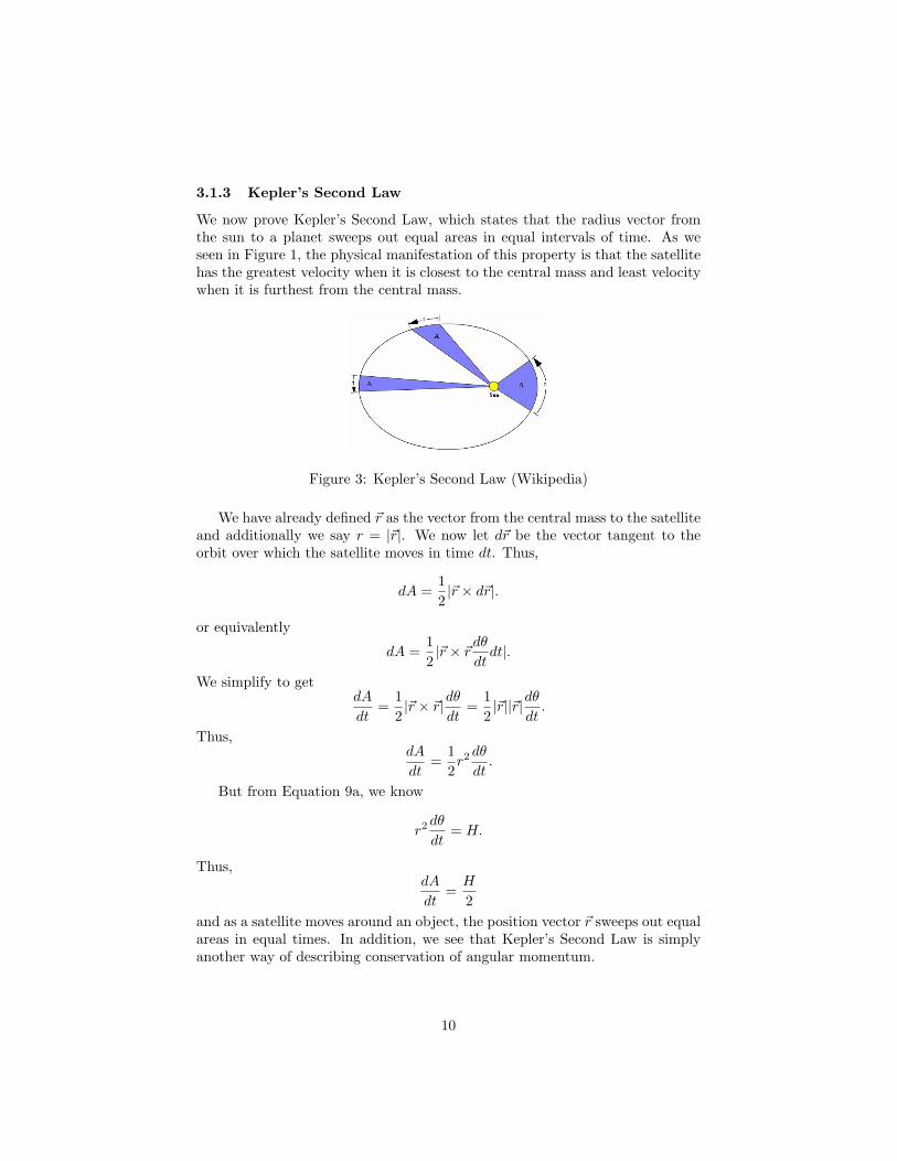
We now prove Kepler’s Second Law, which states that the radius vector fromthe sun to a planet sweeps out equal areas in equal intervals of time. As weseen in Figure 1, the physical manifestation of this property is that the satellitehas the greatest velocity when it is closest to the central mass and least velocitywhen it is furthest from the central mass.

Figure 3: Kepler’s Second Law (Wikipedia)

We have already defined ~r as the vector from the central mass to the satelliteand additionally we say r = |~r|. We now let d~r be the vector tangent to theorbit over which the satellite moves in time dt. Thus,

dA =12|~r × d~r|.

or equivalently

dA =12|~r × ~rdθ

dtdt|.

We simplify to getdA

dt=

12|~r × ~r|dθ

dt=

12|~r||~r|dθ

dt.

Thus,dA

dt=

12r2dθ

dt.

But from Equation 9a, we know

r2dθ

dt= H.

Thus,dA

dt=H

2and as a satellite moves around an object, the position vector ~r sweeps out equalareas in equal times. In addition, we see that Kepler’s Second Law is simplyanother way of describing conservation of angular momentum.

10

3.1.4 Kepler’s Third Law

Finally, we prove Kepler’s Third Law, which states the squares of the periods ofrevolution of the planets around the sun are proportional to the cubes of theirmean distances from the sun. Using Kepler’s Second Law and equation 10a, wehave

dA

dt=

12r2dθ

dt=H

2=

12r0v0 sinα. (16)

In Section 2.2, we showed that the path of a revolving satellite is elliptic.We also know that the area of an ellipse is πab, where a and b are the lengthsof the semi-major axis and semi-minor axis respectively. To find the period ofrevolution T , we integrate equation 16 from t = 0 to t = T yielding

πab = A(T )−A(0) =∫ T

0

dA

dtdt

=∫ T

0

12r0v0 sinαdt

=12r0v0 sinαT. (17)

From our initial conditions for deriving the orbital path and Equation 15b,we have that rmin = pe/(1 + e) occurs when θ = 0 and the maximum valuermax = pe/(1 − e) occurs when θ = π. Therefore the length of the semi-majoraxis, a is

a =max + min

2=

pe

1− e2=

GM2GMr0− v2

0

(18a)

and similarly, the length of the semi-major axis is

b =max−min

2= a

√1− e2 =

v0r0 sinα√2GMr0− v2

0

. (18b)

We can now substitute equations 18a and 18b into equation 17, and obtain theperiod of revolution of the elliptic path of a orbiting satellite,

T =2πGM(

2GMr0− v2

)3/2=

2πa3/2

√GM

(19)

or, to match the wording of the Third Law,

T 2 =4π2a3

GM.

Thus we have Kepler’s Third Law: the square of the period of revolution of aplanet around the sun is proportional to the cube of the mean distance fromthe sun.

11

3.1.5 Orbital Period

We now examine the orbital period of a satellite. We wish to express the time t interms of the angular displacement θ. We cover the major steps of this derivationhere, while the complete derivation is included in Appendix B. We begin withthe statement of conservation of angular momentum in polar coordinates usingthe initial conditions. We have

r2dθ

dt= r0v0 sinα.

We then use the equation for position r in terms of θ,

r =v20r

20 sin2 α/GM

1 + v0r0 sinαGM

√v20 − 2GM

r0+ G2M2

v20r20 sin2 α

cos(θ − θ0).

Substituting for r and rearranging terms yields

dt =v30r

30 sin3 αdθ

G2M2

(1 +

√1− v20r

20 sin2 αG2M2

(2GMr0− v2

0

)cos(θ − θ0)

)2 .

We integrate from 0 to θ and take θ0 = 0, and α = 0, meaning the initialposition is at the perihelion. We have

t =∫ θ

0

v30r

30dθ

G2M2

(1 +

√1− v20r

20 sin2 αG2M2

(2GMr0− v2

0

)cos(θ)

)2 .

From our definition of eccentricity, e, we have

t =∫ θ

0

v30r

30dθ

G2M2 (1 + e cos(θ))2.

In order to evaluate this integral, We begin by multiplying by (1−e2)(1−e2) and

our integral becomes

t =v30r

30

G2M2(1− e2)

∫ θ

0

(1− e2)dθ(1 + e cos(θ))2

.

We now utilize the Weierstrass Substitution

U = tan(θ

2

).

Using properties of trigonometric functions, we find

cos θ =1− U2

1 + U2and sin θ =

2U1 + U2

.

12

We also finddθ =

21 + U2

dU.

We substitute these into our integral to get

v30r

30

G2M2(1− e2)

∫2(1− e2)dU[

1 + e(

1−U2

1+U2

)]2(1 + U2)

.

This integral is equivalent to

v30r

30

G2M2(1− e2)

∫−2e(1 + e) + 2e(1− e)U2

[(1 + e) + (1− e)U2]2dU+

v30r

30

G2M2(1− e2)

∫2

(1 + e) + (1− e)U2dU.

We integrate the first term by reversing the Weierstass substitution andsubsequently using integration by parts. The second term is integrated by usinganother trigonometric substitution. We are then left with

t =v30r

30

G2M2

∫ θ

0

dθ

(1 + e cos(θ))2

=v30r

30

G2M2(1− e2)

[−e sin θ

1 + e cos θ+

2√1− e2

tan−1

[√1− e1 + e

tan(θ

2

)]+ nT

],

where T is the period of the orbit, given by

T =2πa3/2

√GM

and n is the number of complete revolutions the planet has made, or for φ > 2π,φ = θ + 2πn. Thus, the nT term accounts for the planet moving through morethan one complete orbit. As previously mentioned, the complete derivation ofthis equation is presented in Appendix B.

3.2 The Cosmic Velocities

Now that we have proven Kepler’s Laws, we would like to explore some otherresults governing orbits. We begin by finding an equation for the velocity of asatellite at any position r. In our orbital system, we know that the total energyE, given in the equation,

12

[(dr

dt

)2

+ r2(dθ

dt

)2]− GM

r= E,

is constant by the principle of conservation of energy. The first term of thisequation is the kinetic energy of the system, and the second term is the potentialenergy. We can now show that the type of orbit is dependent on the total energyof the system. We begin by recognizing that the square of the velocity is equal

13

to the sum of the squares of the radial and angular components of the velocity.We have (

dr

dt

)2

+ r2(dθ

dt

)2

= v2,

or equivalently,

v2 =2GMr

+ 2E.

We then recall equation 15a

e =

√1− v2

0r20 sin2 α

G2M2

(2GMr0− v2

0

).

Substituting our equation for velocity into the previous equation, we have

e =

√1 +

2v20r

20 sin2 α

G2M2E.

We can now compare the three conditions, E = 0, E < 0, and E > 0. WhenE = 0, we have e = 1, and thus the orbit is parabolic. The condition inwhich E = 0 means that the kinetic energy is equal to the potential energy,which in physical terms means that the object has the minimum amount ofenergy necessary to escape orbit. Because every term in the coefficient of E issquared, we know the coefficient is positive. Thus, for E < 0, we have e < 1and thus the orbit is elliptic. The object does not have sufficient kinetic energyto escape orbit. Similarly, for E > 0, we have e > 1 and therefore the orbit ishyperbolic. Because the kinetic energy is greater than the potential energy, theobject escapes a closed orbit.

We now move on to orbital speed. We have previously established that(dr

dt

)2

+ r2(dθ

dt

)2

= v20 + 2GM

(1r− 1r0

).

This is equivalent to

v2 = v20 + 2GM

(1r− 1r0

)which gives velocity in terms of the initial conditions and the current position.We have also previously shown that

a =GM

2GMr0− v2

0

.

Rearranging terms yields,

v20 =

2GMr0− GM

a.

14

Substituting this statement of our initial conditions into our equation for velocityin terms of r yields

v2 =2GMr0− GM

a+

2GMr− 2GM

r0= GM

(2r− 1a

),

or equivalently,

v =

√GM

(2r− 1a

).

Thus we have an expression for the velocity of a satellite at any position r. Wecan also see that if a = r, a circular orbit, that

v2 =GM

r.

We now demonstrate that the initial propulsion speed v0 of a satellite launchedfrom the Earth’s surface has to fall within a certain range in order for the satel-lite to remain in orbit, which is to say, neither hit the surface of the earth,nor move out of the earth’s gravitational field. We know from the definition ofconic sections, that the size of e in the equation 14 determines the shape of theorbit. We can see from equation 15b that the sign of quantity (v2

0 − 2GM/r0)determines whether e is less than, equal to, or greater than 1. We can thendefine v∗0 as the velocity when e = 1, or

v∗0 =√

2GMr0

=

√2gR2

r0=√R

r0

√2gR, (20)

where g = GMR2 . From equation 15a we can see that when the velocity is less

than the minimum initial velocity, v < v∗0 , then e < 1 and the object will eitherfall back to Earth or orbit elliptically. If v = v∗0 , then e = 1 and the objectwill follow a parabolic path, having just enough energy to escape the Earth’sgravitational field. Finally, if v > v∗0 , then e > 1 and the orbit will be hyperbolic,with the object also escaping the Earth’s gravitational field.

We now know that v0 must be less than√

Rr0

√2gR in order for a satellite to

stay within the gravitational field of the earth. We derive the minimum velocitynecessary for the satellite to stay in orbit. Thus, we are limited by rmin = r0,the point at which the satellite collides with the surface of the earth. We knowrmin = pe/(1 + e) and, using equations 15a and 15b, we have

r0 =1

1 + e

v20r

20 sin2 α

GM, (21a)

which is equivalent to

v20r

20 sin2 α

GM− 1 =

√1− v2

0r20 sin2 α

G2M2

(2GMr0− v2

0

). (21b)

15

The left hand side of equation 21b is always nonnegative, so we have

v0 ≥√GM

r0cscα ≥

√GM

r0=√R

r0

√gR. (22)

Thus we have that the initial speed v0 of a projectile launched from thesurface of the earth must fall within the range,√

R

r0

√gR ≤ v0 ≤

√R

r0

√2gR, r0 > R. (23)

Finally, if we square both sides of equation 21b, we find that sinα = 1 andthus α = π/2. This means that at rmin, the angle between the position vectorand the velocity vector is π/2. Thus, the point where the satellite is closest tothe earth occurs along the major axis. If the satellite is launched with minimumvelocity from this point, the satellite will be further from the earth than rmin

for all other points along its orbit.We now examine an alternative method for deriving the second cosmic ve-

locity, that is the maximum initial velocity an object can be launched from thesurface of a planet and remain in orbit. We previously established that for anobject launched from the planet’s surface to remain in orbit,√

gR < v0 <√

2gR.

The alternative approach is to find the minimum velocity such that the objectwill leave the planet and never return, which is to say that as r increases withoutbound, the velocity remains nonnegative.

We know from F = ma, that

d2y(t)dt2

= −GMr2

.

If we define r = R + y(t) such that R is the radius of the planet and y(t) isthe altitude of the object above the surface of the planet, then our previousequation becomes

d2y(t)dt2

= − R2g

[R+ y(t)]2. (24a)

We can now rearrange terms and solve for the velocity of the object in termsof its height above the surface of the planet. We can rewrite equation 24a as

d[v(t)]dt

= − R2g

[R+ y(t)]2. (24b)

Rearranging terms and multiplying each side of equation 24b by v yields

vdv = −R2g · vdt

[R+ y(t)]2. (25a)

16

We can now use the substitution U = R+ y(t) and thus dU = vdt to get

vdv = −R2g · dUU2

, (25b)

or ∫ v

v0

vdv =∫ y(t)−R

R

−R2g · dUU2

. (25c)

Evaluating this integral, we have

12

(v2 − v20) = R2g

1U

= R2g1

R+ y(t)

∣∣∣y(t)0

. (26a)

This simplifies to

v(t)2 = v20 + 2R2g

[1

R+ y(t)− 1R

]. (26b)

As previously stated, the minimum velocity such that the object never returnsto the planet occurs when the velocity reaches zero as y(t) → ∞. In equation26b, if we let y(t)→∞, we have

v2∞ = v2

0 + 2R2g

[0− 1

R

],

where v∞ is the velocity when y(t) is arbitrarily large. We simplify the previousequation to

v2∞ = v2

0 − 2Rg.

If v∞ > 0 at this point, the object will leave earth. Thus we have

0 < v20 − 2Rg,

orv0 >

√2Rg.

Thus we have verified that the second cosmic velocity is v0 =√

2Rg.

4 Einstein’s Theory of General Relativity

4.1 The Anomalous Advance of Mercury’s Perihelion

For nearly two hundred years after Newton’s Principia was published, the in-verse square law was the accepted method by which to model the motions of theplanets and their satellites. Newton’s Law of Universal Gravitation was evenused by Urbain Jean Joseph Le Verrier to predict the existence of Neptune.By the mid 19th century, however, problems began to arise, most notably withpredictions of the orbit of Mercury. As Le Verrier began his work on the orbitof Mercury, the errors in the prediction of Mercury’s orbit were so large that

17

there was nearly an hour between the predicted and actual start of transit, thetime at which Mercury passes in front of the sun and so can be clearly seen andan accurate position recorded. By 1845, Le Verrier had reduced this error to 16seconds, which was still unacceptable in comparison to the predicted orbits ofother planets (Linton, 437).

Le Verrier discovered that the error in predictions of Mercury’s orbit wasa result of the advance of its perihelion, the closest point on the orbit to theSun. By analyzing the effect of the other planets on the perihelion advance,Le Verrier discovered that Mercury’s perihelion advanced by 565” per centuryrather than the 527” predicted by Newtonian mechanics. Despite this discovery,Le Verrier was unable to explain the cause of the anomalous 38”. (Roseveare,20-37).

Figure 4: Perihelion Advance (Cornell)

Though the problem of Mercury’s orbit was problematic for Newton’s Law ofUniversal Gravitation, the scientific community was not yet willing to questionthe dogma of Newtonian mechanics. Instead other causes of Mercury’s perihe-lion advance were investigated. Based on the success of Le Verrier’s predictionof the existence and position of Neptune, similar techniques were employed inhopes of discovering a planet between the sun and mercury that could be effect-ing the orbit. This hypothetical planet, deemed Vulcan, was “observed” manytimes during the second half of the 19th century, though each discovery wassubsequently discredited (Linton, 441). Alternative hypotheses included thatthe sun was oblate, as well as effects from the ether, the medium through whichlight was thought to travel.

Though models of Mercury’s orbit were now mathematically accurate, deter-mining the cause of the anomaly would require a shift in the way we conceived ofspace and time. Shortly after the start of the 20th century, Einstein had alreadypublished his theory of special relativity, which held that “the laws of physicsare of the same form in all inertial frames, and that in any given inertial frame,the speed of light is the same whether the source is at rest or in uniform motion”(Linton, 454). In response, the mathematician Hermann Minkowski translatedspecial relativity into a geometric framework, and as such created the conceptof four-dimensional spacetime. Within special relativity, which is to say in the

18

absence of a massive object, spacetime, as a four-dimensional Euclidean space,can be thought of as ‘flat.’ Any object moving through this flat spacetime takesthe shortest path and thus travels in a straight line. In developing general rel-ativity, Einstein postulated that mass had the effect of deforming Minkowskianspacetime. An object moving through this deformed space time will still takethe shortest path possible, leading to the elliptical orbit of a planet (Linton,463). The two-dimensional analog of this can be seen in Figure 3, mass deformsflat space time and causes the trajectory of the moving mass to curve.

Figure 5: Mass deforms space time (Carroll)

Unfortunately the mathematical underpinnings of these concepts require aknowledge of tensor calculus and are thus beyond the scope of this paper. Ratherwe will begin with the general relativistic analog of the classical angular mo-mentum and energy equation (previously defined as 11b) derived by simplifyingthe spherically symmetric Swcharzchild solution to Einstein’s field equations.

After developing his gravitational theory, Einstein soon realized that it ex-plained the anomalous advance of Mercury’s perihelion. In correcting the dif-ference between the predicted and observed advance of Mercury’s perihelion,Einstein brought to a close nearly 100 years of mathematical quarreling overthe cause of Mercury’s anomalous perihelion and changed our conception of theuniverse (Roseveare, 147-186).

4.2 Relativistic Angular Momentum and Energy

In order to investigate the effect of General Relativity on the orbit of Mercury, wemust investigate the general-relativity analog of the previously stated classicalangular momentum and energy equation given by(

dr

dt

)2

+ r2(dφ

dt

)2

= v20 + 2GM

(1r− 1r0

). (11b)

19

We let E be a constant related to the energy of the orbit and given by

E =v20

2− GM

r0.

Substituting this into Equation 11b yields(dr

dφ

)2(dφ

dt

)2

+ r2(dφ

dt

)2

= 2Eh2 +2GMr

. (27a)

We also have h, the angular momentum per unit mass given by

h = r2(dφ

dt

).

Dividing by h2, we have

1r4

(dr

dφ

)2

+1r2

=2Eh2

+2GM/r

r4(dφdt

)2 . (27b)

Because energy and angular momentum are conserved, 2Eh2 is a constant which,

for simplicity, we will call E0 and thus we have

1r4

(dr

dφ

)2

+1r2

= E0 +2GM/r

r4(dφdt

)2 . (27c)

We then introduce the substitution u = 1r , and thus du = −drr2 . This yields(

du

dφ

)2

+ u2 = E0 +2GMh2

u. (27d)

This is the classical angular momentum and energy equation. In solving Ein-stein’s field equations, which is beyond the scope of this project, a generalrelativistic analog of the previous equation is derived. We find that the gen-eral relativistic equation is the classical equation with another term, equal to2GMu3/c2. We expect that this term will change the orbit of a satellite frompure Keplerian motion. We then have the equation(

du

dφ

)2

+ u2 = E0 +2GMh2

u+2GMu3

c2. (28a)

The quantity 2GM/c2 is small compared to the radius of planetary orbits. Wecan denote this quantity as ε, and we have(

du

dφ

)2

+ u2 = E0 +2GMh2

u+ εu3. (28b)

20

Aphelion and Perihelion occur where du/dφ = 0, and thus we have

εu3 − u2 +(

2GMh2

)u+ E0 = 0. (29)

This cubic equation then has three roots, let them be denoted u1, u2, and u3.Because ε is small, unless u is large, the roots will be close to the roots of theanalogous classical equation

u2 −(

2GMh2

)u− E0 = 0.

Thus, we say u1 and u2 are close to the roots of the Newtonian model and thuswe let u1 be the aphelion and u2 be the perihelion. Thus we know u1 ≤ u ≤ u2.We also know that u1 + u2 + u3 = 1/ε. For a proof of this see appendix C.Because 1/ε is large, u3 is also large and thus has no physical meaning in ourmodel. Substituting our solution for equation 29 into equation 28a, we have

du

dφ= [ε(u− u1)(u2 − u)(u3 − u)]

12 . (30a)

Rearranging terms, we have

du

dφ= [[(u− u1)(u2 − u)(ε(u3 − u))]

12 .

We then rewrite this as

du

dφ= [[(u− u1)(u2 − u)(ε(u1 − u1 + u2 − u2 + u3 − u))]

12 .

We then group terms such that

du

dφ= [[(u− u1)(u2 − u)(ε(u1 + u2 + u3)− ε(u1 + u2 + u)))]

12 .

We can cancel ε and u1 + u2 + u3. This yields

du

dφ= [[(u− u1)(u2 − u)(1− ε(u1 + u2 + u)))]

12 .

In terms of dφ/du, we have

dφ

du=

1[(u− u1)(u2 − u)]1/2

[1− ε(u1 + u2 + u)]−1/2. (30b)

Using the first order approximation from the Taylor expansion, (1 + x)k =1 + kx, we have

dφ

du≈

1 + 12ε(u1 + u2 + u)

[(u− u1)(u2 − u)]1/2. (30c)

21

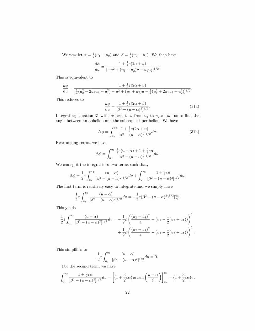
We now let α = 12 (u1 + u2) and β = 1

2 (u2 − u1). We then have

dφ

du=

1 + 12ε(2α+ u)

[−u2 + (u1 + u2)u− u1u2]1/2.

This is equivalent to

dφ

du=

1 + 12ε(2α+ u)

[ 14 (u22 − 2u1u2 + u2

1)− u2 + (u1 + u2)u− 14 (u2

1 + 2u1u2 + u22)]1/2

.

This reduces todφ

du=

1 + 12ε(2α+ u)

[β2 − (u− α)2]1/2. (31a)

Integrating equation 31 with respect to u from u1 to u2 allows us to find theangle between an aphelion and the subsequent perihelion. We have

∆φ =∫ u2

u1

1 + 12ε(2α+ u)

[β2 − (u− α)2]1/2du. (31b)

Rearranging terms, we have

∆φ =∫ u2

u1

12ε(u− α) + 1 + 3

2εα

[β2 − (u− α)2]1/2du.

We can split the integral into two terms such that,

∆φ =12ε

∫ u2

u1

(u− α)[β2 − (u− α)2]1/2

du+∫ u2

u1

1 + 32εα

[β2 − (u− α)2]1/2du.

The first term is relatively easy to integrate and we simply have

12ε

∫ u2

u1

(u− α)[β2 − (u− α)2]1/2

du = −12ε(β2 − (u− α)2)1/2|u2

u1.

This yields

12ε

∫ u2

u1

(u− α)[β2 − (u− α)2]1/2

du =− 12ε

((u2 − u1)2

4− (u2 −

12

(u2 + u1)))2

+12ε

((u2 − u1)2

4− (u1 −

12

(u2 + u1)))2

.

This simplifies to12ε

∫ u2

u1

(u− α)[β2 − (u− α)2]1/2

du = 0.

For the second term, we have∫ u2

u1

1 + 32εα

[β2 − (u− α)2]1/2du =

[(1 +

32εα) arcsin

(u− αβ

)]u2

u1

= (1 +32εα)π.

22

Doubling ∆φ and subtracting 2π gives the angle between successive perihelions.We then have that each orbit advances the perihelion by

φ = 3εαπ =3GMπ

c2(u1 + u2) =

3GMπ

c2

(1r1

+1r2

), (32)

where r1 and r2 are the values of r at aphelion and perihelion. In the case ofMercury, r1 and r2 are small compared to orbital radii of the other planets.As a result, Mercury has a larger perihelion advance then the other planets..In addition, because the orbit of Mercury is more elliptical than the orbits ofmost of the other planets, aphelion and perihelion are easier to observe. ForMercury, the advancement of perihelion works out to about 43” per century.While small, it is enough to be observed, and previous to Einstein’s Theory ofGeneral Relativity, was unexplainable.

5 Conclusion

In this paper, we began by verifying Kepler’s Laws of Planetary Motion usingNewton’s Law of Universal Gravitation. We then derived several results per-taining to the orbital period of a satellite, including solving for orbital period interms of angular displacement. We then derived an equation for the velocity of asatellite, as well as the cosmic velocities, the minimum and maximum velocitiesnecessary for a satellite to stay in orbit. Finally, we examined the anomalousorbit of Mercury using Newton’s Law of Universal Gravitation and Einstein’sTheory of Relativity.

In our use of classical mechanics in exploring planetary motion, we assumedseveral things. First, we assumed that we have a two-body system, using theexample of a satellite orbiting Earth. In reality, a massive body’s orbit is per-turbed by the gravitational attraction to any other mass in its vicinity. Thus,the orbits of the planets are not simply two-body systems with a given planetorbiting the Sun, rather the orbit of each planet is affected by the other plan-ets. Unfortunately, this multiple-body problem is very complicated and mustbe modeled numerically. Fortunately, the Sun is vastly more massive than theplanets and thus the two-body model is a reasonable approximation. Our secondassumption was that the Earth is is a homogeneous sphere rather than a hetero-geneous ellipsoid. The ellipsoidal shape of the Earth causes small perturbationsof the elliptic path of a satellite.

Additional considerations include that the perihelion advance of Mercury’sorbit is not simply due to the effects of General Relativity. The gravitationaleffects of other planets, as well as the fact that we are observing Mercury froma moving platform, contribute to Mercury’s perihelion advance. In our analysiswe simply derived the additional orbital advance that was discovered by LeVerrier and explained by General Relativity.

Our analysis also assumes no knowledge of tensor calculus in the deriva-tion of Mercury’s perihelion advance from the relativistic angular momentum

23

and energy equation. Given an understanding of tensor calculus, the angularmomentum and energy equation can be derived from Einstein’s field equations.

Reasonable areas for further work would be deriving additional results per-taining to the orbits of individual satellites as well as analysis of the three-bodyproblem. A useful resource for additional work in this area is Solar SystemDynamics by Carl D. Murray and Stanley F. Dermott. Given an understandingof tensor calculus, the angular momentum and energy equation could also bederived, as well as other results in General Relativity. A useful resource for addi-tional work in this area is A Short Course in General Relativity as referenced inthe bibliography. Further information on the historical context of the mathemat-ics covered in the paper can be found in From Eudoxus to Einstein: A Historyof Mathematical Astronomy as referenced in the bibliography.

24

6 Appendices

6.1 Appendix A

On page 7, we used the standard process of completing the square to transformequation 12b into equation 12c. The full derivation is given here. We beginwith equation 12b

−dθ =v0r0 sinαdz√(

v20 − 2GM

r0

)+ 2GMz − v2

0r20 sin2 αz2

. (12b)

The denominator is

(v20r

20 sin2 α)z2 − (2GM)z +

(2GMr0− v2

0

).

This is equivalent to(v0r0 sinαz − GM

v0r0 sinα

)2

+ C,

where C is some constant that we will determine. We then expand the abovestatement, yielding

(v20r

20 sin2 α)z2 − (2GM)z +

G2M2

v20r

20 sin2 α

+ C.

Equating this statement with the square of the denominator of equation 12band simplifying we have

G2M2

v20r

20 sin2 α

+ C =2GMr0− v2

0 .

Solving for C, we have

C =2GMr0− v2

0 −G2M2

v20r

20 sin2 α

.

We then find a common denominator, which gives us

C =2GMv2

0r0 sin2 α− v40r

20 sin2 α−G2M2

v20r

20 sin2 α

.

Thus equation 12b becomes

−dθ =v0r0 sinαdz√

(G2M2−2GMv20r0 sin2 α+v40r20 sin2 α)

v20r20 sin2 α

−(v0r0 sinαz − GM

v0r0 sinα

)2. (12c)

25

6.2 Appendix B

In section 2.1.5, we examined the orbital period of a satellite and found anequation for the time t in terms of the angular displacement θ. The completederivation is presented here. We begin with the statement of conservation ofangular momentum in polar coordinates using the initial conditions. We have

r2dθ

dt= r0v0 sinα.

We then use the equation for position r in terms of θ,

r =v20r

20 sin2 α/GM

1 + v0r0 sinαGM

√v20 − 2GM

r0+ G2M2

v20r20 sin2 α

cos(θ − θ0).

Substituting for r yields v40r

40 sin4 α/G2M2(

1 + v0r0 sinαGM

√v20 − 2GM

r0+ G2M2

v20r20 sin2 α

cos(θ − θ0))2

dθdt

= r0v0 sinα.

Rearranging terms, we have

dt =v30r

30 sin3 αdθ

G2M2(

1 + v0r0 sinαGM

√v20 − 2GM

r0+ G2M2

v20r20 sin2 α

cos(θ − θ0))2 .

Again we rearrange terms, which yields

dt =v30r

30 sin3 αdθ

G2M2

(1 +

√v40r

20 sin2 αG2M2 − 2v20r0 sin2 α

GM + 1 cos(θ − θ0))2 .

This is equivalent to

dt =v30r

30 sin3 αdθ

G2M2

(1 +

√1− v20r

20 sin2 αG2M2

(2GMr0− v2

0

)cos(θ − θ0)

)2 .

For θ0 = 0, and α = 0, meaning the initial position is the perihelion, we have

t =∫ θ

0

v30r

30dθ

G2M2

(1 +

√1− v20r

20 sin2 αG2M2

(2GMr0− v2

0

)cos(θ)

)2 .

From our definition of eccentricity, e, we finally have

t =∫ θ

0

v30r

30dθ

G2M2 (1 + e cos(θ))2.

26

In order to evaluate this integral, We begin by multiplying by (1−e2)(1−e2) such

that our integral becomes

t =v30r

30

G2M2(1− e2)

∫ θ

0

(1− e2)dθ(1 + e cos(θ))2

.

We now utilize the Weierstrass Substitution such that

U = tan(θ

2

).

We can use properties of trigonometric functions to find expressions forcos(θ), sin(θ), and dθ. We begin with cos θ and we know that

U2 =1− cos θ1 + cos θ

.

We now rewrite this equation, and we have

U2 + U2 cos θ = 1− cos θcos θ + U2 cos θ = 1− U2

(1 + U2) cos θ = 1− U2

cos θ =1− U2

1 + U2

To find an expression for sin θ, we begin with

sin2 θ = 1− cos2 θ

sin2 θ = 1−(

1− U2

1 + U2

)2

sin2 θ =1 + 2U2 + U2

(1 + U2)2− 1− 2U2 + U2

(1 + U2)2

sin2 θ =4U2

(1 + U2)2

and we havesin θ =

2U1 + U2

.

To find dθ, we can use the derivative of sin θ. We then have

cos θdθ =(1 + U2) · 2− (2U)(2U)

(1 + U2)2dU.

We then have

dθ =(1 + U2) · 2− (2U)(2U)

(1 + U2)21 + U2

1− U2dU.

27

This simplifies to

dθ =2

1 + U2dU.

We can now substitute into our integral. This yields

v30r

30

G2M2(1− e2)

∫2(1− e2)dU[

1 + e(

1−U2

1+U2

)]2(1 + U2)

.

Rearranging terms, we have

v30r

30

G2M2(1− e2)

∫2(1− e2)dU[

(1+U2)+e(1−U2)1+U2

]2(1 + U2)

.

This simplifies to

v30r

30

G2M2(1− e2)

∫2(1− e2)(1 + U2)dU[(1 + e) + (1− e)U2]2

.

Expanding the numerator, we have

v30r

30

G2M2(1− e2)

∫2(1− e2 + U2 − e2U2)dU

[(1 + e) + (1− e)U2]2.

We can rewrite the numerator, yielding

v30r

30

G2M2(1− e2)

∫2(1− e2) + 2(1− e2)U2

[(1 + e) + (1− e)U2]2dU.

Factoring yields

v30r

30

G2M2(1− e2)

∫2(1 + e)(1− e) + 2(1 + e)(1− e)U2

[(1 + e) + (1− e)U2]2dU.

We now rewrite the numerator as

v30r

30

G2M2(1− e2)

∫−2e(1 + e) + 2(1 + e) + 2e(1− e)U2 + 2(1− e)U2

[(1 + e) + (1− e)U2]2dU.

We can now separate this into two terms

v30r

30

G2M2(1− e2)

∫−2e(1 + e) + 2e(1− e)U2

[(1 + e) + (1− e)U2]2dU+

v30r

30

G2M2(1− e2)

∫2(1 + e) + 2(1− e)U2

[(1 + e) + (1− e)U2]2dU.

The second term reduces, and we have

v30r

30

G2M2(1− e2)

∫−2e(1 + e) + 2e(1− e)U2

[(1 + e) + (1− e)U2]2dU+

v30r

30

G2M2(1− e2)

∫2

(1 + e) + (1− e)U2dU.

28

We begin by integrating the first term,

v30r

30

G2M2(1− e2)

∫−2e(1 + e) + 2e(1− e)U2

[(1 + e) + (1− e)U2]2dU.

We rewrite this as

=v30r

30

G2M2(1− e2)

∫−2e[(1 + e)− (1− e)U2]

[(1 + e) + (1− e)U2]2

(1 + U2

2

)(2

1 + U2

)dU.

Expanding the numerator, we have

=v30r

30

G2M2(1− e2)

∫−e[(1 + e) + (1 + e)U2 − (1− e)U2 − (1− e)U4]

[(1 + e) + (1− e)U2]2

(2

1 + U2dU

).

This is equivalent to

=v30r

30

G2M2(1− e2)

∫−e[(1 + e) + U2 + 2eU2 − U2 − (1− e)U4]

[(1 + e) + (1− e)U2]2

(2

1 + U2dU

).

Rearranging terms in the numerator yields

=v30r

30

G2M2(1− e2)

∫−e[(1− U4) + e− 2eU2 + eU4 + 4eU2]

[(1 + e) + (1− e)U2]2

(2

1 + U2dU

).

We now factor terms in the numerator and have

=v30r

30

G2M2(1− e2)

∫−e(1− U2)(1 + U2)− e2(1− U2)(1− U2)− e(2U)2

[(1 + e) + (1− e)U2]2

(2

1 + U2dU

).

We now multiply by(

1+U2

1+U2

)2

such that we have

=v30r

30

G2M2(1− e2)

∫ −e(1−U2)(1+U2)−e2(1−U2)(1−U2)−e(2U)2

(1+U2)2[(1+U2

1+U2

)+ e

(1−U2

1+U2

)]2 (2

1 + U2dU

).

We then rearrange terms, which yields

=v30r

30

G2M2(1− e2)

∫ −e( 1−U2

1+U2

)− e2

(1−U2

1+U2

)2

− e2(

2U1+U2

)2

[1 + e

(1−U2

1+U2

)]2 (2

1 + U2dU

).

We can combine the first and second terms of the numerator such that

=v30r

30

G2M2(1− e2)

∫ −e( 1−U2

1+U2

) [1 + e

(1−U2

1+U2

)]− e2

(2U

1+U2

)2

[1 + e

(1−U2

1+U2

)]2 (2

1 + U2dU

).

29

We can now substitute for cos θ, sin θ, dθ. This yields

=v30r

30

G2M2(1− e2)

∫(1 + e cos θ)(−e cos θ)− (−e sin θ)(−e sin θ)

(1 + e cos θ)2dθ.

Splitting the integral into two terms, we have

=v30r

30

G2M2(1− e2)

[−∫

e cos θ1 + e cos θ

dθ −∫

e2 sin2 θ

(1 + e cos θ)2dθ

].

We begin integration by parts on the second term such that

U = e sin θ dU = e cos θdθ

V = 11+e cos θ dV = e sin θ

(1+e cos θ)2 dθ

We now have

=v30r

30

G2M2(1− e2)

[−∫

e cos θ1 + e cos θ

dθ − e sin θ1 + e cos θ

+∫

e cos θ(1 + e cos θ)

dθ

].

The first and third terms cancel and we are left with

=v30r

30

G2M2(1− e2)−e sin θ

1 + e cos θ.

We now integrate the second term,

v30r

30

G2M2(1− e2)

∫2

(1 + e) + (1− e)U2dU.

We multiply this by√

1−e√1−e and 1+e

1+e such that we have

=v30r

30

G2M2(1− e2)

∫ 2√

1−e√1−e

1+e√1+e√

1+e

(1 + e) + (1− e)U2dU.

Rearranging terms yields

=v30r

30

G2M2(1− e2)

∫ 2√1−e√

1+e

(√1−e√1+e

)[

(1+e)+(1−e)U2

1+e

] dU.

This is equivalent to

=v30r

30

G2M2(1− e2)2√

1− e√

1 + e

∫ (√1−e√1+e

)1 +

(√1−e√1+e

U)2 dU.

30

We now introduce another trigonometric substitution such that

U =

√1 + e

1− etan(V ) dU =

√1 + e

1− esec2(V )dV.

Substituting, we have

=v30r

30

G2M2(1− e2)2√

1− e√

1 + e

∫sec2(V )

1 + tan2(V )dV.

We know sec2(V ) = 1 + tan2(V ), and so we reduce and integrate yielding

=v30r

30

G2M2(1− e2)2√

1− e√

1 + e

∫dV =

v30r

30

G2M2(1− e2)2√

1− e√

1 + e· V.

Substituting for V yields

=v30r

30

G2M2(1− e2)2√

1− e2tan−1

(√1− e1 + e

U

).

Substituting for U , we have

=v30r

30

G2M2(1− e2)2√

1− e2tan−1

[√1− e1 + e

tan(θ

2

)].

Finally, we have

t =v30r

30

G2M2

∫ θ

0

dθ

(1 + e cos(θ))2

=v30r

30

G2M2(1− e2)

[−e sin θ

1 + e cos θ+

2√1− e2

tan−1

[√1− e1 + e

tan(θ

2

)]+ nT

],

where T is the period of the orbit, given by

T =2πa3/2

√GM

and n is the number of complete revolutions the planet has made, or for φ > 2π,φ = θ + 2πn.

6.3 Appendix C

Proving u1 + u2 + u3 = 1ε .

When we expand ε(u−u1)(u2−u)(u3−u), the u2 term works out to be −ε(u1 +u2 + u3)u2. Equating this with the u2 term in our energy equation, we have−ε(u1 + u2 + u3)u2 = −u2, and thus

u1 + u2 + u3 =1ε.

31

7 Bibliography

Carroll, Sean M. “Spacetime and Geometry: An Introduction to GeneralRelativity.” Preposterous Universe. California Institute of Technology.5 May 2009. http://preposterousuniverse.com/spacetimeandgeometry/

Foster, James and J.D. Nightingale. A Short Course in General Relativity. 1st.London, Longman Mathematical Texts, 1979.

Kwok, Yue-Kuen. “Motion of an Artificial Satellite About the Earth.”Undergraduate Mathematics and its Applications Project695(1989): 130-147.

Linton, C.M. From Eudoxus to Einstein: A History of Mathematical Astronomy.1st. Cambridge, UK: Cambridge UP, 2004.

Roseveare, N.T. Mercury’s Perihelion: From Le Verrier to Einstein. 1st.Oxford, UK: Oxford UP, 1982.

“The Advance of the Perihelion of Mercury.” Cornell University Dept. ofAstronomy. 5 May 2009.http://www.astro.cornell.edu/academics/courses/astro201/merc adv.htm

32