Senate Bill 350 Study

Senate Bill 350 Study Volume X: Disadvantaged Community Impact Analysis PREPARED FOR

PREPARED BY

July 8, 2016

Copyright © 2016 Aspen Environmental Group and Berkeley Economic Advising & Research, LLC

Senate Bill 350 Study The Impacts of a Regional ISO-Operated Power Market on California

List of Report Volumes

Executive Summary

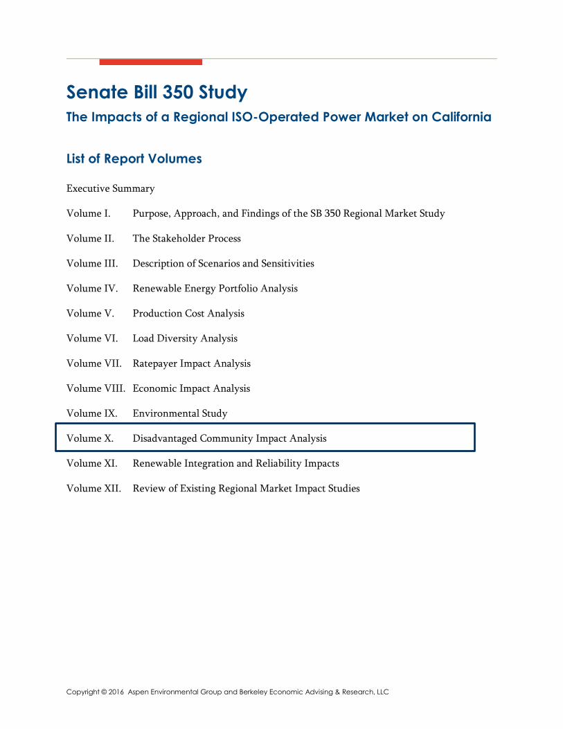
Volume I. Purpose, Approach, and Findings of the SB 350 Regional Market Study

Volume II. The Stakeholder Process

Volume III. Description of Scenarios and Sensitivities

Volume IV. Renewable Energy Portfolio Analysis

Volume V. Production Cost Analysis

Volume VI. Load Diversity Analysis

Volume VII. Ratepayer Impact Analysis

Volume VIII. Economic Impact Analysis

Volume IX. Environmental Study

Volume X. Disadvantaged Community Impact Analysis

Volume XI. Renewable Integration and Reliability Impacts

Volume XII. Review of Existing Regional Market Impact Studies

Senate Bill 350 Study

Volume X

Disadvantaged Community Impact Analysis

Prepared by:

Aspen Environmental Group

Berkeley Economic Advising and Research

July 2016

SB 350 Evaluation and Plan VOLUME X. DISADVANTAGED COMMUNITY IMPACT ANALYSIS

July 2016 X-i

Volume X: Table of Contents 1. Screening for Disadvantaged Communities - Overview ........................................................................ X-1

1.1 Definition of Disadvantaged Communities ................................................................................. X-2 1.2 Determination of Disadvantaged Communities .......................................................................... X-2

2. Disadvantaged Communities Identified ................................................................................................. X-6 2.1 CalEnviroScreen Score and Maps ................................................................................................ X-6 2.2 Disadvantaged Communities for the Environmental Analysis .................................................... X-8 2.3 Disadvantaged Communities for the Economic Analysis .......................................................... X-16

3. Ranking of Disadvantaged Communities ............................................................................................. X-16

4. Environmental Impacts in Disadvantaged Communities ..................................................................... X-18 4.1 Typical Community-Scale Impacts of the Buildouts .................................................................. X-23 4.2 Environmental Impacts of Regionalization in Disadvantaged Communities ............................ X-27

5. Economic Impact in Disadvantaged Communities ............................................................................... X-33 5.1 Methodology for Determining Economic Impacts in Disadvantaged Communities ................. X-33 5.2 Economic Impact Results .......................................................................................................... X-34

6. Comparison of Scenarios ..................................................................................................................... X-47 6.1 Environmental Comparison of Scenarios .................................................................................. X-47 6.2 Economic Comparison of Scenarios .......................................................................................... X-48

7. References ........................................................................................................................................... X-48

8. Annex A: Disadvantaged Community Figures for Additional Economic Regions................................. X-49

Tables Table 1. CalEnviroScreen Indicators Used for Identifying Disadvantaged Communities .......................... X-3 Table 2. CalEnviroScreen Indicators and Data Sources .............................................................................. X-3 Table 3. CalEnviroScreen Scores by County ............................................................................................. X-12 Table 4. CalEnviroScreen Scores by Air Basin .......................................................................................... X-14 Table 5. CalEnviroScreen Scores by Aggregated CREZ ............................................................................. X-15 Table 6. Disadvantaged Community Aggregation Used for Economic Analysis ...................................... X-16 Table 7. Air Basins with the Highest-Scoring Disadvantaged Communities ............................................ X-17 Table 8. CREZs with the Highest-Scoring Disadvantaged Communities .................................................. X-17 Table 9. Economic Regions with the Highest-Scoring Disadvantaged Communities ............................... X-18 Table 10. Water Use for Electricity Production in California ................................................................... X-30 Table 11. NOx Emissions Changes, California Natural Gas Fleet by Air Basin ......................................... X-31 Table 12. PM2.5 Emissions Changes, California Natural Gas Fleet by Air Basin ...................................... X-31 Table 13. SO2 Emissions Changes, California Natural Gas Fleet by Air Basin .......................................... X-32

Figures Figure 1. CalEnviroScreen 2.0 Scores by County ........................................................................................ X-9 Figure 2. CalEnviroScreen 2.0 Scores by Air Basin ................................................................................... X-10 Figure 3. CalEnviroScreen 2.0 Scores by Aggregated CREZ ...................................................................... X-11 Figure 4. Disadvantaged Communities Focus Map 1 ............................................................................... X-20 Figure 5. Disadvantaged Communities Focus Map 2 ............................................................................... X-21


July 2016 X-ii

Figure 6. Disadvantaged Communities Focus Map 3 ............................................................................... X-22 Figure 7. Downscaling Results to Identify Impacts in Disadvantaged Communities ............................... X-33 Figure 8. Job Creation Across Scenarios in Disadvantaged Communities and Non-Disadvantaged Communities ............................................................................................................................................ X-35 Figure 9. Difference in Job Creation Across Scenarios in Disadvantaged Communities and Non-Disadvantaged Communities ................................................................................................................... X-36 Figure 10. Difference in Community Income Across Scenarios in Disadvantaged Communities and Non-Disadvantaged Communities ........................................................................................................... X-37 Figure 11. Difference in FTE Jobs in Disadvantaged Communities .......................................................... X-38 Figure 12. Difference in FTE Jobs in Disadvantaged Communities (Inland Valley) .................................. X-39 Figure 14. Difference in FTE Jobs in Disadvantaged Communities (Central Valley) ................................ X-41 Figure 15. Differences in Disadvantaged Community Income ................................................................. X-42 Figure 16. Differences in Disadvantaged Community Income – Inland Valley ........................................ X-44 Figure 17. Differences in Disadvantaged Community Income – Greater Los Angeles ............................ X-45 Figure 18. Differences in Disadvantaged Community Income – Central Valley ...................................... X-46


July 2016 X-1

Volume X. Disadvantaged Communities Impact Analysis California’s Senate Bill No. 350—the Clean Energy and Pollution Reduction Act of 2015 — (SB 350) requires the California Independent System Operator (CAISO, Existing ISO, or ISO) to conduct one or more studies of the impacts of a regional market enabled by governance modifications that would transform the ISO into a multistate or regional entity (Regional ISO). SB 350, in part, specifically requires an evaluation of “impacts in disadvantaged communities in California.” Aspen Environmental Group and Berkeley Economic Advising and Research have been engaged to study these impacts. This report is Volume X of XII of an overall study in response to SB 350’s legislative requirements.

This report begins by defining disadvantaged communities, identifies them by location, and presents environmental and economic assessments of energy policy impacts on them. Aspen Environmental Group conducted the environmental study, and Berkeley Economic Advising and Research (BEAR) conducted the economic assessment. More detailed information on methodologies and assumptions, and on impacts across the entire study region, including areas outside of disadvantaged communities, can be found in the Environmental Study (Volume IX) and in the Economic Impact Analysis (Volume VIII).

As discussed in detail below, the limited regionalization in 2020 causes no adverse environmental impact in California’s disadvantaged communities and may result in small but beneficial environmental effects by generally reducing water use and NOx emissions. Modeling of the 2020 CAISO + PAC scenario indicates that the San Joaquin Valley and South Coast air basins could slightly increase PM2.5 and SO2 emissions due to changes in the dispatch of natural gas-fired power plants, but these changes would occur in conjunction with a NOx decrease.

The most severely disadvantaged communities from an economic perspective lie in three regions: Los Angeles (56%), Central Valley (22%), and Inland Valley (13%). For these communities, there are economic benefits right from the start of regionalization in 2020. For 2030, the current practice results in a renewable buildout impacting seven solar resource areas and six different wind resource areas, including four that have a high level of concern for impacts to disadvantaged communities (Westlands; Central Valley North & Los Banos; Kramer & Inyokern; Greater Imperial). The Regional 2 and Regional 3 buildout by 2030 occurs across a smaller number of resource areas in California, when compared with Current Practice 1, although two buildout areas have a high level of concern for impacts to disadvantaged communities (Kramer & Inyokern; Greater Imperial). Thus with expanded regionalization and increased renewable buildout out of state, the impact to California’s disadvantaged communities would decline. Regional 2 and Regional 3 both produce more jobs in 2030 in disadvantaged communities than Current Practice 1, arising primarily from job growth induced by ratepayer savings. The economic analysis also considers how income effects differ between disadvantaged and non-disadvantaged communities across scenarios. Once again the state trend with Regional 2 shows the largest increases in incomes and employment across both disadvantaged and non-disadvantaged communities.

1. Screening for Disadvantaged Communities - Overview

The methodology begins with an initial screening of California’s disadvantaged communities through maps and tables. The study of disadvantaged communities is limited to California and does not consider out of state effects or out-of-state communities.


July 2016 X-2

1.1 Definition of Disadvantaged Communities

The term “disadvantaged community” is associated with minority and low-income populations in several California laws (e.g., Safe Drinking Water Act, Affordable Housing and Sustainable Communities Program [Public Resources Code, Division 44, Part 1, Section 75200]). Additionally, in 2012 the California Legislature passed Senate Bill 535 (De León), regarding the Greenhouse Gas Reduction Fund, which required the California Environmental Protection Agency (CalEPA) to implement a more comprehensive approach to identifying disadvantaged communities in California through the use of public health and environmental hazard criteria in addition to socioeconomic data (CalEPA, 2014). Through this refined approach, the state definition of disadvantaged communities was expanded to include areas that are disproportionately impacted by environmental pollution and negative public health effects.

This study uses current California definitions and tools to define a disadvantaged community as an area that is:

Disproportionately affected by environmental pollution and other hazards that can lead to negative public health effects, exposure, or environmental degradation; and/or

Characterized by concentrations of people that are of low income, high unemployment, low levels of home ownership, high rent burden, sensitive health, or low levels of educational attainment.

1.2 Determination of Disadvantaged Communities

Implementing the provisions of SB 535 is a multi-agency effort among the California Environmental Protection Agency (CalEPA), the Office of Environmental Health Hazard Assessment (OEHHA), and the Air Resources Board (ARB) (ARB, 2016). In addition to targeting a statewide reduction of greenhouse gas emissions, SB 535 earmarked 25 percent of the Greenhouse Gas Reduction Fund for projects that provide a benefit to disadvantaged communities. The CalEPA was tasked with the responsibility for identifying disadvantaged communities for the purpose of SB 535. CalEPA developed CalEnviroScreen (California Communities Environmental Health Screening Tool) as a science-based tool for evaluating multiple pollutants and stressors in communities, and ultimately for identifying disadvantaged communities (CalEPA, 2014).

CalEnviroScreen uses existing environmental, public health, and socioeconomic data to develop indicators to create a screening score for communities across the state. An area with a high score would be expected to experience more severe environmental impacts than areas with low scores. CalEnviroScreen 2.0 (updated October 2014) uses a quantitative method to evaluate multiple pollution sources and stressors, and vulnerability to pollution, in California’s approximately 8,000 U.S. Census Tracts. Using data from federal and state sources, the tool consists of indicators (Table 1) that are divided into two broad groups:

Indicators for exposure and environmental effects comprise a Pollution Burden group; and

Indicators for sensitive populations and socioeconomic factors comprise a Population Characteristics group.


July 2016 X-4

Table 2. CalEnviroScreen Indicators and Data Sources

Issue Indicator Data Source Diesel Particulate Matter

Spatial distribution of gridded diesel PM emissions from on-road and non-road sources for a 2010 summer day in July (kg/day)

California Air Resources Board San Diego Association of Governments

Drinking Water Contaminants

Drinking water contaminant index for selected contaminants

Public Water System Location Data (PICME Database), CDPH Safe Drinking Water Information System, U.S.

EPA Water Quality Monitoring Database, CDPH Domestic Well Project, Groundwater Ambient

Monitoring and Assessment (GAMA) Program, State Water Resources Control Board (SWRCB) Priority Basin Project, GAMA Program, SWRCB

and U.S. Geological Survey

Pesticide Use Total pounds of selected active pesticide ingredients (filtered for hazard and volatility) used in production-agriculture per square mile

Pesticide Use Reporting, California Department of Pesticide Regulation

Toxic Releases from Facilities

Toxicity-weighted concentrations of modeled chemical releases to air from facility emissions and off-site incineration

Risk Screening Environmental Indicators U.S. EPA Toxic Release Inventory

Traffic Density Sum of traffic volumes adjusted by road segment length (vehicle-kilometers per hour) divided by total road length (kilometers) within 150 meters of the census tract boundary

Environmental Health Investigations Branch, CDPH San Diego Association of Governments

Cleanup Sites Sum of weighted sites within each census tract

EnviroStor Cleanup Sites Database, Department of Toxic Substances Control (DTSC) US EPA, Region 9 NPL Sites (Superfund Sites)

Polygons

Groundwater Threats

Sum of weighted scores for sites within each census tract

GeoTracker Database, SWRCB

Hazardous Waste Generators and Facilities

Sum of weighted permitted hazardous waste facilities and hazardous waste generators within each census tract

EnviroStor Hazardous Waste Facilities Database and Hazardous Waste Tracking System, DTSC

Impaired Water Bodies

Summed number of pollutants across all water bodies designated as impaired within the area

303(d) List of Impaired Water Bodies, SWRCB

Solid Waste Sites and Facilities

Sum of weighted solid waste sites and facilities

Solid Waste Information System and Closed, Illegal, and Abandoned Disposal Sites Program, California Department of Resources Recycling and Recovery, CalRecycle


July 2016 X-6

CalEnviroScreen Score and Maps

The CalEnviroScreen 2.0 model uses the following formula to calculate an overall CalEnviroScreen Score for a particular census tract:

(Pollution Burden) x (Populations Characteristics) = CalEnviroScreen Score

As demonstrated in the above formula, the CalEnviroScreen Score is calculated by multiplying the Pollution Burden score with the Populations Characteristics score. Since each of the two groups (i.e., Pollution Burden and Populations Characteristics) has a maximum score of 10, the maximum CalEnviroScreen Score is 100.

Additional considerations involved with the CalEnviroScreen system and scoring include:

Geographic Resolution of Data: CalEnviroScreen 2.0 (utilized within this report) uses census tract boundary data for the 2010 Census obtained from the U.S. Census Bureau.

Indicator Data Criteria: Data must be available statewide at the census tract level geographical unit or translatable to the census tract level; must be of sufficient quality; and must be complete, accurate, and current.

Score Calculation Method for Pollution Burden and Population Characteristics Groups:

– First, the percentiles for all the individual indicators in a group are averaged. Within the Pollution Burden Group, indicators from the environmental effects component are weighted half as much as indicators from the exposures component.2 Thus, the score for the Pollution Burden category is a weighted average, with exposure indicators receiving twice the weight as environmental effects indicators.

– Second, Pollution Burden and Population Characteristics percentile averages are scaled so that they have a maximum value of 10 and a possible range of 0 to 10. Each average is divided by the maximum value observed in the state and then multiplied by 10. The scaling ensures that the pollution component and population component contribute equally to the overall CalEnviroScreen score.

2. Disadvantaged Communities Identified

2.1 CalEnviroScreen Score and Maps

Using CalEnviroScreen, the disadvantaged census tracts within California have been identified. Because this tool is California-specific, it provides the following advantages for an in-state analysis:

Use of census tracts3 as the geographic scale allows for a reasonably precise screening of pollution burdens and vulnerabilities in specific communities.

The tool reflects CalEPA’s continued effort to enhance the current indicators by incorporating the most up-to-date information, as available.

2 The contribution to possible pollutant burden from the environmental effects indicators is considered to be less

than those from sources in the exposures indicators, and therefore a weighted average is used to calculate the total Pollution Burden.

3 Census tracts generally have a population size between 1,200 and 8,000 people, with an optimum size of 4,000 people (approximately 1,500 housing units) (USCB, 2015).


July 2016 X-7

Disadvantaged Communities Identified Statewide

Once CalEnviroScreen scores are calculated for each census tract, these tracts are ordered from highest to lowest, based on their overall score. After taking into consideration legislative direction, comparative markers of being disadvantaged and basic principles of fairness, CalEPA has decided on the use of a 25 percent threshold to identify disadvantaged communities (CalEPA, 2014). All census tracts (and population within) ranked within the top 25 percentile are considered disadvantaged within a statewide context.

CalEPA developed maps that show the percentiles for all the state’s census tracts and that highlight the census tracts that are within the top 25 percent of communities. CalEnviroScreen scores within the top 25 percent, which are defined as disadvantaged communities, correspond to percentile as follows:

Score of 7.51 to 8 represents 75 to 80%;

Score of 8.1 to 9 represents 81 to 90% (population within this ranking is considered more sensitive than that ranked 75 to 80%); and

Score of 9.1 to 10 represents 91 to 100% (population within this ranking is considered more sensitive than that ranked 75 to 90%).

Disadvantaged Communities Overlay Boundaries for SB 350 Study

In the maps and tables presented with this methodology overview, the locations of disadvantaged communities within the State of California appear, along with an overlay of the following three boundaries for comparison purposes:

County boundaries.

Air Basin boundaries. California is divided geographically into air basins for the purpose of managing the air resources of the state on a regional basis. An air basin generally has similar meteorological and geographic conditions throughout. California is currently divided into 15 air basins.

Competitive Renewable Energy Zone (CREZ) boundaries. CREZ boundaries are established under the Renewable Energy Transmission Initiative (RETI) process and identify the best renewable resource locations to prioritize future transmission infrastructure development. An Aggregated CREZ is a coarsely-defined geography that can span multiple counties or substantial portions of counties.

Information is provided for the 25% highest-scoring census tracts within California, as these census tracts contain the population considered to be disadvantaged that could bear disproportionate impacts from energy infrastructure siting. Because the overlay boundaries encompass complete census tracts and portions of census tracts, to avoid double-counting population in partial tracts, the counted population and number of tracts considers the census tracts that are primarily within each of the boundaries. Accordingly, population data presented here includes some portion outside each overlay boundary.

Note that the scores for each area identified by CalEnviroScreen are the same underlay for each map in this overview, only the overlay of the different boundary types change here (i.e., County, Air Basin, and CREZ).


July 2016 X-8

2.2 Disadvantaged Communities for the Environmental Analysis

Disadvantaged Communities in California by County

Figure 1 shows the distribution of the top 25% highest CalEnviroScreen scores across the counties in California. Table 3 (at the end of this section) provides data corresponding to the map, and shows the population levels in disadvantaged communities by county. As shown in Table 3, the counties with the highest percentages of population in disadvantaged communities are: Merced, Tulare, Fresno, Kings, Madera, Kern, Imperial, San Joaquin, Stanislaus, Los Angeles, and San Bernardino.

Disadvantaged Communities in California Air Basins

Figure 2 shows the distribution of the top 25% highest CalEnviroScreen scores across air basins in California. Table 4 (at the end of this section) provides data corresponding to the map, and shows the population levels in disadvantaged communities by air basin. As shown in Table 4, the San Joaquin Valley, South Coast, and Salton Sea air basins contain the highest percentages of population in disadvantaged communities.

Disadvantaged Communities in CREZs

Figure 3 shows the distribution of the top 25% highest CalEnviroScreen scores across the Aggregated CREZs in this overview. Table 5 (at the end of this section) provides data corresponding to the map, and shows the population levels in disadvantaged communities by CREZ. As shown in Table 5, the Westlands, Central Valley North & Los Banos, Mountain Pass & El Dorado, Kramer & Inyokern, and Greater Imperial CREZs contain the highest percentages of population in disadvantaged communities.

SB 3

50 E

valu

atio

n an

d Pl

an

V OLU

ME

X. D

ISAD

VAN

TAG

ED C

OM

MU

NIT

Y IM

PACT

AN

ALYS

IS

July

201

6 X-

9

Figu

re 1

. Cal

Envi

roSc

reen

2.0

Sco

res

by C

ount

y

SB 3

50 E

valu

atio

n an

d Pl

an

V OLU

ME

X. D

ISAD

VAN

TAG

ED C

OM

MU

NIT

Y IM

PACT

AN

ALYS

IS

July

201

6 X-

10

Figu

re 2

. Cal

Envi

roSc

reen

2.0

Sco

res

by A

ir B

asin

SB 3

50 E

valu

atio

n an

d Pl

an

V OLU

ME

X. D

ISAD

VAN

TAG

ED C

OM

MU

NIT

Y IM

PACT

AN

ALYS

IS

July

201

6 X-

11

Figu

re 3

. Cal

Envi

roSc

reen

2.0

Sco

res

by A

ggre

gate

d C

REZ

SB 3

50 E

valu

atio

n an

d Pl

an

V OLU

ME

X. D

ISAD

VAN

TAG

ED C

OM

MU

NIT

Y IM

PACT

AN

ALYS

IS

July

201

6 X-

12

Tabl

e 3.

Cal

Envi

roSc

reen

Sco

res b

y Co

unty

Coun

ty

76-8

0% H

ighe

st S

core

s 81

-90%

Hig

hest

Sco

res

91-1

00%

Hig

hest

Sco

res

Coun

ty T

otal

s (t

op 2

5% h

ighe

st sc

orin

g ar

eas)

Perc

enta

ge o

f Co

unty

Pop

ulat

ion

with

in

Disa

dvan

tage

d Co

mm

uniti

es

No.

of

Trac

ts

Popu

latio

n

No.

of

Trac

ts

Popu

latio

n

No.

of

Trac

ts

Popu

latio

n

No.

of

Trac

ts

Popu

latio

n Pe

rcen

tage

M

erce

d 5

27,9

44

17

97,5

44

14

62,1

52

36

187,

640

73%

Fr

esno

14

70

,293

36

17

2,20

4 81

38

6,22

3 13

1 62

8,72

0 68

%

Tula

re

7 43

,448

26

12

3,00

2 17

11

0,76

9 50

27

7,21

9 63

%

Mad

era

2 17

,424

6

36,5

84

5 38

,016

13

92

,024

61

%

Kern

18

97

,718

24

12

8,41

6 31

20

2,27

1 73

42

8,40

5 51

%

Stan

islau

s 10

51

,793

20

92

,520

20

98

,543

50

24

2,85

6 47

%

Los A

ngel

es

163

674,

588

408

1,76

2,56

9 44

7 1,

910,

843

1018

4,

348,

000

44%

Sa

n Jo

aqui

n 10

42

,512

26

13

4,42

9 28

12

0,93

9 64

29

7,88

0 43

%

San

Bern

ardi

no

23

119,

125

61

343,

508

76

400,

063

160

862,

696

42%

Ki

ngs

2 8,

795

7 28

,136

5

25,8

87

14

62,8

18

41%

Im

peria

l 6

33,1

52

7 36

,482

—

—

13

69

,634

40

%

Rive

rsid

e 30

14

5,31

7 32

17

5,00

4 42

20

7,53

0 10

4 52

7,85

1 24

%

Ora

nge

33

213,

508

43

249,

509

10

63,8

40

86

526,

857

18%

Yu

ba

—

—

3 12

,296

—

—

3

12,2

96

17%

Sa

cram

ento

15

67

,461

19

92

,340

9

36,7

88

43

196,

589

14%

Co

ntra

Cos

ta

13

68,0

18

10

53,1

86

—

—

23

121,

204

12%

Yo

lo

1 4,

922

1 7,

702

1 5,

397

3 18

,021

9%

M

onte

rey

3 15

,783

3

15,1

39

1 4,

518

7 35

,440

9%

Al

amed

a 15

55

,909

16

62

,896

1

5,54

7 32

12

4,35

2 8%

Te

ham

a 1

4,11

2 —

—

—

—

1

4,11

2 6%

Sa

nta

Clar

a 7

29,4

76

13

67,3

57

3 8,

771

23

105,

604

6%

Butt

e 3

12,3

13

—

—

—

—

3 12

,313

6%

Ve

ntur

a 3

9,07

6 2

9,00

2 3

15,3

90

8 33

,468

4%

SB 3

50 E

valu

atio

n an

d Pl

an

V OLU

ME

X. D

ISAD

VAN

TAG

ED C

OM

MU

NIT

Y IM

PACT

AN

ALYS

IS

July

201

6 X-

13

Tabl

e 3.

Cal

Envi

roSc

reen

Sco

res b

y Co

unty

Coun

ty

76-8

0% H

ighe

st S

core

s 81

-90%

Hig

hest

Sco

res

91-1

00%

Hig

hest

Sco

res

Coun

ty T

otal

s (t

op 2

5% h

ighe

st sc

orin

g ar

eas)

Perc

enta

ge o

f Co

unty

Pop

ulat

ion

with

in

Disa

dvan

tage

d Co

mm

uniti

es

No.

of

Trac

ts

Popu

latio

n

No.

of

Trac

ts

Popu

latio

n

No.

of

Trac

ts

Popu

latio

n

No.

of

Trac

ts

Popu

latio

n Pe

rcen

tage

Sa

n Di

ego

8 40

,549

14

60

,614

4

15,4

32

26

116,

595

4%

Sant

a Cr

uz

1 7,

976

—

—

—

—

1 7,

976

3%

Sola

no

1 2,

962

1 8,

423

—

—

2 11

,385

3%

Sa

nta

Barb

ara

1 11

,406

—

—

—

—

1

11,4

06

3%

San

Mat

eo

1 7,

510

1 7,

327

—

—

2 14

,837

2%

Sa

n Fr

anci

sco

2 7,

546

1 3,

499

—

—

3 11

,045

1%

No

te: T

he co

unted

popu

lation

and n

umbe

r of tr

acts

includ

e the

cens

us tr

acts

that a

re pr

imar

ily w

ithin

each

boun

dary

and m

ay no

t inclu

de th

e pop

ulatio

n of th

e par

tial tr

acts

in ea

ch ov

erlay

boun

dary.

SB 3

50 E

valu

atio

n an

d Pl

an

V OLU

ME

X. D

ISAD

VAN

TAG

ED C

OM

MU

NIT

Y IM

PACT

AN

ALYS

IS

July

201

6 X-

14

Tabl

e 4.

Cal

Envi

roSc

reen

Sco

res b

y Ai

r Bas

in

Air B

asin

76-8

0% H

ighe

st S

core

s 81

-90%

Hig

hest

Sco

res

91-1

00%

Hig

hest

Sco

res

Air B

asin

Tot

als

(top

25%

hig

hest

sc

orin

g ar

eas)

Perc

enta

ge o

f Air

Basi

n Po

pula

tion

with

in

Disa

dvan

tage

d Co

mm

uniti

es

No.

of

Trac

ts

Popu

latio

n

No.

of

Trac

ts

Popu

latio

n

No.

of

Trac

ts

Popu

latio

n

No.

of

Trac

ts

Popu

latio

n Pe

rcen

tage

Sa

n Jo

aqui

n Va

lley

67

354,

453

162

812,

835

201

1,04

4,80

0 43

0 2,

212,

088

58%

Sout

h Co

ast

242

1,11

2,09

7 53

4 2,

469,

914

575

2,58

2,27

6 1,

351

6,16

4,28

7 39

%

Salto

n Se

a 9

57,5

47

9 50

,060

—

—

18

10

7,60

7 18

%

Sacr

amen

to V

alle

y 20

88

,808

24

12

0,76

1 10

42

,185

54

25

1,75

4 9%

Moj

ave

Dese

rt

5 21

,520

8

47,0

98

—

—

13

68,6

18

7%

Nor

th C

entr

al C

oast

4

23,7

59

3 15

,139

1

4,51

8 8

43,4

16

6%

San

Fran

cisc

o Ba

y 39

17

1,42

1 40

19

0,81

5 4

14,3

18

83

376,

554

5%

San

Dieg

o Co

unty

8

40,5

49

14

60,6

14

4 15

,432

26

11

6,59

5 4%

Sout

h Ce

ntra

l Coa

st

4 20

,482

2

9,00

2 3

15,3

90

9 44

,874

3%

Grea

t Bas

in V

alle

ys

—

—

—

—

—

—

0 0

0%

Note:

The

coun

ted po

pulat

ion an

d num

ber o

f trac

ts inc

lude t

he ce

nsus

trac

ts tha

t are

prim

arily

with

in ea

ch bo

unda

ry an

d may

not in

clude

the p

opula

tion o

f the p

artia

l trac

ts in

each

over

lay bo

unda

ry.

SB 3

50 E

valu

atio

n an

d Pl

an

V OLU

ME

X. D

ISAD

VAN

TAG

ED C

OM

MU

NIT

Y IM

PACT

AN

ALYS

IS

July

201

6 X-

15

Tabl

e 5.

Cal

Envi

roSc

reen

Sco

res b

y Ag

greg

ated

CRE

Z

Aggr

egat

ed C

REZ

76-8

0% H

ighe

st S

core

s 81

-90%

Hig

hest

Sco

res

91-1

00%

Hig

hest

Sco

res

CREZ

Tot

als

(top

25%

hig

hest

sc

orin

g ar

eas)

Perc

enta

ge o

f Po

pula

tion

with

in C

REZ

with

in

Disa

dvan

tage

d Co

mm

uniti

es

No.

of

Trac

ts

Popu

latio

n

No.

of

Trac

ts

Popu

latio

n

No.

of

Trac

ts

Popu

latio

n

No.

of

Trac

ts

Popu

latio

n Pe

rcen

tage

W

estla

nds

42

232,

204

99

488,

342

139

763,

166

280

1,48

3,71

2 62

%

Cent

ral V

alle

y N

& L

os B

anos

15

79

,737

37

19

0,06

4 34

16

0,69

5 86

43

0,49

6 56

%

Kram

er &

Inyo

kern

22

11

5,27

9 61

34

3,50

8 76

40

0,06

3 15

9 85

8,85

0 42

%

Grea

ter I

mpe

rial

6 33

,152

7

36,4

82

—

—

13

69,6

34

22%

Sola

no

55

241,

784

72

355,

526

39

168,

671

166

765,

981

15%

Rive

rsid

e Ea

st &

Pal

m S

prin

gs

4 27

,736

2

13,5

78

—

—

6 41

,314

9%

Sout

hern

Cal

iforn

ia D

eser

t 1

3,84

6 —

—

—

—

1

3,84

6 8%

Teha

chap

i 2

8,40

7 2

10,9

00

—

—

4 19

,307

2%

Nor

ther

n Ca

lifor

nia

4 16

,425

—

—

—

—

4

16,4

25

2%

Grea

ter C

arriz

o 1

11,4

06

—

—

—

—

1 11

,406

2%

Ow

ens V

alle

y &

Inyo

—

—

—

—

—

—

0

0 0%

No

te: T

he co

unted

popu

lation

and n

umbe

r of tr

acts

includ

e the

cens

us tr

acts

that a

re pr

imar

ily w

ithin

each

boun

dary

and m

ay no

t inclu

de th

e pop

ulatio

n of th

e par

tial tr

acts

in ea

ch ov

erlay

boun

dary.


July 2016 X-16

2.3 Disadvantaged Communities for the Economic Analysis

The economic and environmental analyses use the same criteria for identifying disadvantaged communities; however, the economic analysis uses an alternative aggregation methodology for reporting results. Disadvantaged communities are aggregated to nine multi-county economic regions (Table 6). 91% of California’s disadvantaged communities fall within three economic regions: Los Angeles (56%), Central Valley (22%), and Inland Valley (13%).

Table 6. Disadvantaged Community Aggregation Used for Economic Analysis

Regions Counties within Region

Percent of Disadvantaged Communities

Los Angeles Los Angeles, Ventura, Orange 56%

Central Valley San Joaquin, Stanislaus, Merced, Madera, Fresno, Kings, Tulare, Kern, Mariposa, Tuolumne, Calaveras, Amador 22%

Inland Valley San Bernardino, Riverside 13%

Bay Area San Francisco, Marin, Sonoma, Napa, Solano, Contra Costa, Alameda, Santa Clara, San Mateo 4%

Sacramento El Dorado, Placer, Sacramento, Yolo, Sutter, Yuba 2.5%

San Diego and Imperial San Diego, Imperial 2%

Central Coast Monterey, San Luis Obispo, Santa Barbara, Santa Cruz, San Benito <1%

North State Del Norte, Siskiyou, Modoc, Humboldt, Trinity, Shasta, Lassen, Tehama, Plumas, Sierra, Nevada, Butte, Glenn, Colusa, Lake, Mendocino <1%

Southern Sierra Alpine, Mono, Inyo None Note: The nine economic region aggregation is taken from the following report by the California EPA Office of Environmental Health Hazard

Assessment: Approaches to Identifying Disadvantaged Communities (2014).

3. Ranking of Disadvantaged Communities

Areas that have the greatest numbers of highest-scoring tracts according to CalEnviroScreen results are considered in this study to be the areas of greatest concern. The areas of greatest concern in this study are likely to have many census tracts in the highest-scoring decile, and the highest percentage of population in disadvantaged communities, as shown previously for the air basins (Table 4), the CREZs (Table 5), and Economic Regions (Table 6).

The geographic resolution of the environmental study is at the scale of air basins and CREZs, some of which include hundreds of census tracts defined as disadvantaged communities The number of census tracts that are disadvantaged communities, meaning those in the highest quartile of CalEnviroScreen scores (7.6-10), and the number of census tracts with the highest decile of CalEnviroScreen Scores (9.1-10) are used here to further focus the study on areas where highest-scoring tracts are most likely to occur. Any area that has more than 40% of census tracts the top quartile also in the top decile (i.e., more than 10 tracts in the top decile per every 25 tracts in the top quartile) is an area characterized with the highest-scoring tracts.

Table 7 lists the air basins with the number of tracts in the highest-scoring decile and fraction of disadvantaged communities that are the highest-scoring. Table 7 shows that the San Joaquin Valley and South Coast air basins have the greatest numbers of the highest-scoring disadvantaged communities.


July 2016 X-17

On the basis of having a relatively high percentage of population in disadvantaged communities (Table 4), the top three air basins of greatest concern also include the Salton Sea air basin.

Table 7. Air Basins with the Highest-Scoring Disadvantaged Communities

Air Basin

Percentage of Air Basin Population

within Disadvantaged Communities

CalEnviroScreen Scores between

7.6 and 10 (No. of Tracts

in Top Quartile)


9.1 and 10 (No. of Tracts in Top Decile)

Highest-Scoring Areas

(Top Decile divided by Top Quartile)

San Joaquin Valley 58% 430 201 47%

South Coast 39% 1,351 575 43% South Central Coast 3% 9 3 33%

Sacramento Valley 9% 54 10 19% San Diego County 4% 26 4 15%

North Central Coast 6% 8 1 13% San Francisco Bay 5% 83 4 5%

Salton Sea 18% 18 0 0%

Mojave Desert 7% 13 0 0% Note: The counted number of tracts considers the census tracts that are primarily within each boundary, shown also in Table 4.

Table 8 lists the CREZs with number of tracts in the highest-scoring decile and fraction of disadvantaged communities that are the highest-scoring. The top five CREZs of greatest concern include the Central Valley North & Los Banos and Greater Imperial CREZs, due to a relatively high percentage of population in disadvantaged communities; the Solano CREZ has a lower percentage of population in disadvantaged communities (Table 5). Table 8 shows that the Westlands and Kramer & Inyokern CREZs also have the greatest numbers of highest-scoring disadvantaged communities.

Table 8. CREZs with the Highest-Scoring Disadvantaged Communities

Aggregated CREZ

Percentage of Population

within CREZ within Disadvantaged Communities


7.6 and 10 (No. of Tracts

in Top Quartile)


9.1 and 10 (No. of Tracts in Top Decile)

Highest-Scoring Areas

(Top Decile divided by Top Quartile)

Westlands 62% 280 139 50% Kramer & Inyokern 42% 159 76 48% Central Valley N & Los Banos 56% 86 34 40%

Solano 15% 166 39 23% Greater Imperial 22% 13 0 0% Riverside East & Palm Springs 9% 6 0 0%

Southern California Desert 8% 1 0 0%

Northern California 2% 4 0 0% Tehachapi 2% 4 0 0% Greater Carrizo 2% 1 0 0% Note: The counted number of tracts considers the census tracts that are primarily within each boundary, shown also in Table 5.


July 2016 X-18

Table 9 lists the nine economic regions with the number of disadvantaged communities the top decile and quartile of CalEnviroScreen scores; 91% of the disadvantaged communities are in Central Valley, Inland Valley, and Los Angeles. These are also the three economic regions with the greatest number of high-scoring disadvantaged communities.

Table 9. Economic Regions with the Highest-Scoring Disadvantaged Communities

Aggregated Economic Region

CalEnviroScreen Scores between 9.1 and 10

(No. of Tracts in Top Decile)

CalEnviroScreen Scores between 7.6 and 10

(No. of Tracts in Top Quartile)

Highest-Scoring Areas (Top Decile divided

by Top Quartile) Central Valley 201 431 47% Inland Valley 118 264 45% Los Angeles 460 1,112 41% Sacramento 10 49 20% Central Coast 1 9 11% San Diego and Imperial 4 39 10% Bay Area 4 85 5% North State 0 4 0% Southern Sierra 0 0 NA

In summary, the areas having the highest percentages of population in disadvantaged communities and the highest-scoring disadvantaged communities are:

Air Basins: the San Joaquin Valley, South Coast, and Salton Sea air basins.

CREZs: the Westlands, Central Valley North & Los Banos, Kramer & Inyokern, and Greater Imperial CREZs.

Economic Regions: the Central Valley, Inland Valley, and Los Angeles economic regions.

4. Environmental Impacts in Disadvantaged Communities

For our environmental study of impacts in disadvantaged communities, we focus on whether the action of changing the California ISO into a regional market operator is likely to increase the environmental pollution burden on any disadvantaged community. Two criteria are used here to describe how the different regionalization scenarios can affect disadvantaged communities:

First, because regionalization is likely to influence the preferred locations for the incremental renewable energy buildout to meet California’s 50% Renewable Portfolio Standard (RPS), construction of the buildout and long-term operation of renewable energy facilities may create adverse community-scale effects depending on whether the buildout is located in a setting of disadvantaged communities. The impacts common to all portfolios and the incremental buildout to meet the RPS by 2030 are discussed in Section 4.1.

Second, because regionalization is likely to cause changes in the operation of the existing system of generation, and because power production may consume water and create emissions of air pollutants, the regional differences in power production are reviewed for adverse effects in areas of disadvantaged communities. The operational impacts are summarized in Section 4.2.

The potential to increase the pollution burden in disadvantaged communities could occur:


July 2016 X-19

If the locations of the incremental renewable energy buildout shift to identified disadvantaged communities under regionalization.

If the location of an adverse environmental impact shifts to an area that predominately includes disadvantaged communities under regionalization.

Because the specific locations of community-scale impacts depend on the locations of actual individual future projects, these impacts cannot be determined with certainty at this time. However, the discussion below presents the typical localized environmental impacts resulting from renewable energy and utility-scale transmission project construction and operation that could affect areas of disadvantaged communities.

Figures 4, 5, and 6 illustrate the relative capacity that would be added by each buildout and the locations of disadvantaged communities in their resource zones.

SB 3

50 E

valu

atio

n an

d Pl

an

V OLU

ME

X. D

ISAD

VAN

TAG

ED C

OM

MU

NIT

Y IM

PACT

AN

ALYS

IS

July

201

6 X-

20

Figu

re 4

. Dis

adva

ntag

ed C

omm

unit

ies

Focu

s M

ap 1

SB 3

50 E

valu

atio

n an

d Pl

an

V OLU

ME

X. D

ISAD

VAN

TAG

ED C

OM

MU

NIT

Y IM

PACT

AN

ALYS

IS

July

201

6 X-

21

Figu

re 5

. Dis

adva

ntag

ed C

omm

unit

ies

Focu

s M

ap 2

SB 3

50 E

valu

atio

n an

d Pl

an

V OLU

ME

X. D

ISAD

VAN

TAG

ED C

OM

MU

NIT

Y IM

PACT

AN

ALYS

IS

July

201

6 X-

22

Figu

re 6

. Dis

adva

ntag

ed C

omm

unit

ies

Focu

s M

ap 3


July 2016 X-23

4.1 Typical Community-Scale Impacts of the Buildouts

This study of environmental impacts in disadvantaged communities considers how regionalization may influence the preferred locations for the incremental renewable energy buildout and how those locations may relate to disadvantaged communities. Because construction of the buildout and long-term operation of renewable energy facilities may create adverse community-scale effects depending on whether the buildout is located in a setting of disadvantaged communities, this section describes the environmental impacts that would be common across the scenarios as a result of the incremental buildout by 2030.

Note that the SB 350 environmental study is not site-specific and does not reflect or represent a siting study for any particular planned or conceptual construction project. Although environmental impacts are described in general, project-specific impacts can typically be managed through best management practices and mitigation, through the siting processes and with review by the siting authorities.

Construction Impacts in General

Common types of environmental impacts resulting from construction of large-scale renewable energy facilities or transmission infrastructure expansions could occur within disadvantaged communities depending on project-specific circumstances. These types of construction activities are similar for the incremental renewable energy buildouts in all scenarios. Therefore, the discussions below describe the types of impacts that could occur on a community-scale for construction of renewable energy facilities and associated transmission interconnections, with technology-specific unique or distinguishing aspects mentioned. Because construction is limited in duration, the potential to create construction-related environmental impacts essentially ends with the end of construction. These construction-phase impacts can typically be managed by siting authorities through best management practices and mitigation.

General types of construction impacts include:

Air Quality: The typical construction-related air quality impacts are caused by fugitive dust from grading, vehicles driving on unpaved surfaces or roadways, and emissions from heavy-duty construction equipment and vehicles carrying construction materials and workers. These emissions occur during site development and preparation, transmission line development, and from building and roadway construction. The types of emissions would be the same for each renewable energy technology.

Construction activities may include mobilization, land clearing, earth moving, road construction, ground excavation, drilling and blasting, foundation construction, and installation activities. Heavy equipment used during site preparation would also include bulldozers, scrapers, trucks, cranes, rock drills, and possibly blasting equipment. These activities and equipment use would temporarily increase the amounts of particulate matter, including PM2.5, and precursors to particulate matter. Similarly, increased amounts of ozone precursors (volatile organic compounds [VOCs] and nitrogen oxides [NOx]) would occur from engine exhaust emissions, further exacerbating ozone nonattainment conditions.

Increased health risks would result for people exposed to excessive concentrations of dust, potentially including valley fever, and hazardous or toxic air pollutants routinely caused by gasoline and diesel-powered equipment. Diesel particulate matter is designated as a toxic air contaminant in California. High levels of construction-phase emissions can exacerbate regional nonattainment conditions or expose sensitive receptors to substantial concentrations of hazardous or toxic air pollutants during project construction. Assessing the air quality impacts from construction emissions usually involves


July 2016 X-24

project-specific quantification of air pollutants emitted by construction activities for each phase of site development for each project.

Noise: Temporary construction noise typically occurs intermittently and varies depending on the nature or phase of construction (e.g., demolition and land clearing, grading and excavation, erection). Construction noise is localized and can create short term nuisances from the activities such as site preparation, trucks hauling material, concrete pouring, use of power tools, etc. Noise from heavy-duty equipment, including earthmovers, material handlers, and portable generators, can reach high levels for brief periods. Temporary noise impacts would be similar for all renewable energy types.

Traffic: During construction of renewable energy and transmission facilities, workers commute to the project site over local roads, and shipments to and from the facilities are usually by truck. Rail transport to the closest intermodal facility for materials could also be used. The movement of persons, equipment, and materials to project sites during construction could cause a temporary decrease in the performance levels on local primary and secondary road networks.

Wind turbine components are delivered in oversized or overweight loads, such as the rotor blades, which may be delivered as one piece, and nacelles, which contain massive drivetrain components and generators. Transporting these components typically requires permitting for movement of oversized loads and temporary road closures. In addition, the main cranes required for tower and turbine assembly typically also require a number of oversized or overweight shipments. The wind energy transportation requirements may cause temporary disruptions in surrounding communities.

Operational Impacts in General

General types of impacts that occur over the long-term operation of large-scale renewable energy facilities or transmission infrastructure expansions include:

Aesthetics: The operation and maintenance of renewable energy facilities and associated transmission lines, roads, and rights-of-way would have long-term adverse visual effects due to visual intrusion of facilities introduced into landscapes. Among these are land scarring, introduction of structural contrast and industrial elements into natural settings, view blockage, and skylining (silhouetting of elements against the sky). Another impact common to renewable energy facilities is dust generated by vehicle movement within a site or along a right-of-way or access road. Without proper disturbed soil management strategies, wind can mobilize dust from project sites and create visible plumes or clouds of dust.

Solar projects introduce geometric shapes and repeated linear elements into the visual environment. Utility-scale projects have a large footprint and are usually in open and relatively flat settings with little to no vegetative or other screening. Solar energy projects also vary in their visual impacts because of the different technologies employed. Furthermore, the level of impact can vary between urban and rural landscapes. While more viewers in urban areas see solar installations, the installations will typically create greater visual contrast in rural areas. Under certain viewing conditions, solar installations give rise to specular reflections (glint and glare) visible to stationary or moving observers from long distances, and can constitute a major source of visual impact. Glint and glare from photovoltaic facilities are typically lower than solar concentrating facilities using trough, power tower, and solar dish technologies that employ mirrors and lenses.

Wind energy projects are usually highly visible because the vertical towers and rotating turbine blades need unobstructed access to the wind resource, usually best in areas where there are few, if any, comparable tall structures in strongly horizontal landscapes. Visual impacts associated with the


July 2016 X-25

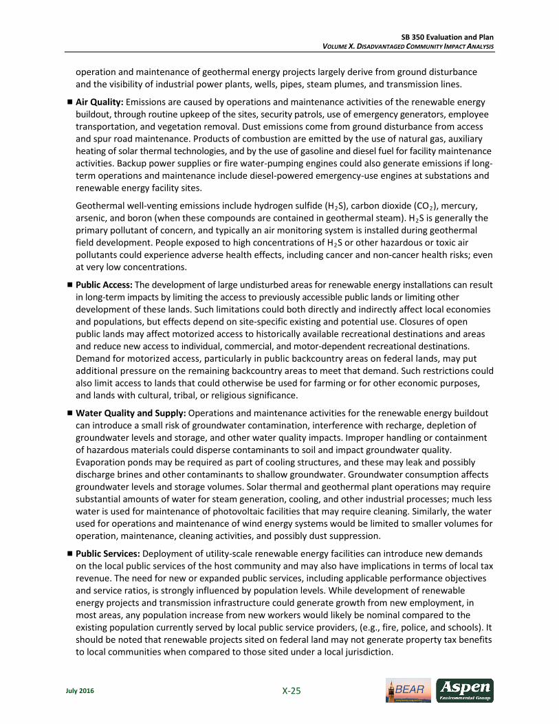
operation and maintenance of geothermal energy projects largely derive from ground disturbance and the visibility of industrial power plants, wells, pipes, steam plumes, and transmission lines.

Air Quality: Emissions are caused by operations and maintenance activities of the renewable energy buildout, through routine upkeep of the sites, security patrols, use of emergency generators, employee transportation, and vegetation removal. Dust emissions come from ground disturbance from access and spur road maintenance. Products of combustion are emitted by the use of natural gas, auxiliary heating of solar thermal technologies, and by the use of gasoline and diesel fuel for facility maintenance activities. Backup power supplies or fire water-pumping engines could also generate emissions if long-term operations and maintenance include diesel-powered emergency-use engines at substations and renewable energy facility sites.

Geothermal well-venting emissions include hydrogen sulfide (H2S), carbon dioxide (CO2), mercury, arsenic, and boron (when these compounds are contained in geothermal steam). H2S is generally the primary pollutant of concern, and typically an air monitoring system is installed during geothermal field development. People exposed to high concentrations of H2S or other hazardous or toxic air pollutants could experience adverse health effects, including cancer and non-cancer health risks; even at very low concentrations.

Public Access: The development of large undisturbed areas for renewable energy installations can result in long-term impacts by limiting the access to previously accessible public lands or limiting other development of these lands. Such limitations could both directly and indirectly affect local economies and populations, but effects depend on site-specific existing and potential use. Closures of open public lands may affect motorized access to historically available recreational destinations and areas and reduce new access to individual, commercial, and motor-dependent recreational destinations. Demand for motorized access, particularly in public backcountry areas on federal lands, may put additional pressure on the remaining backcountry areas to meet that demand. Such restrictions could also limit access to lands that could otherwise be used for farming or for other economic purposes, and lands with cultural, tribal, or religious significance.

Water Quality and Supply: Operations and maintenance activities for the renewable energy buildout can introduce a small risk of groundwater contamination, interference with recharge, depletion of groundwater levels and storage, and other water quality impacts. Improper handling or containment of hazardous materials could disperse contaminants to soil and impact groundwater quality. Evaporation ponds may be required as part of cooling structures, and these may leak and possibly discharge brines and other contaminants to shallow groundwater. Groundwater consumption affects groundwater levels and storage volumes. Solar thermal and geothermal plant operations may require substantial amounts of water for steam generation, cooling, and other industrial processes; much less water is used for maintenance of photovoltaic facilities that may require cleaning. Similarly, the water used for operations and maintenance of wind energy systems would be limited to smaller volumes for operation, maintenance, cleaning activities, and possibly dust suppression.

Public Services: Deployment of utility-scale renewable energy facilities can introduce new demands on the local public services of the host community and may also have implications in terms of local tax revenue. The need for new or expanded public services, including applicable performance objectives and service ratios, is strongly influenced by population levels. While development of renewable energy projects and transmission infrastructure could generate growth from new employment, in most areas, any population increase from new workers would likely be nominal compared to the existing population currently served by local public service providers, (e.g., fire, police, and schools). It should be noted that renewable projects sited on federal land may not generate property tax benefits to local communities when compared to those sited under a local jurisdiction.


July 2016 X-26

Environmental Benefits

The construction and operation of large-scale renewable energy facilities may also provide environmental benefits, which can reduce preexisting burdens within disadvantaged communities. In general, the greatest beneficial impacts result from renewable energy facilities leading to a reduction or avoidance of the natural resources used by or emitted as a result of operating conventional power plants.

Regulatory precedent for identifying the environmental benefits of California’s renewable energy buildout appears in SB X1-2, signed in 2011, that was reiterated in SB 350. According to SB X1-2 [specifically, in Pub. Util. Code § 399.13(a)(7)], procurement of renewable energy should give preference “to renewable energy projects that provide environmental and economic benefits to communities afflicted with poverty or high unemployment, or that suffer from high emission levels of toxic air contaminants, criteria air pollutants, and greenhouse gases.”

General types of beneficial impacts that could occur from the incremental renewable energy buildout include:

Air Quality: Producing electricity from the renewable energy resources displaces the need to produce electricity and the associated air contaminants from conventional fossil fuel-fired power generation facilities. While such benefits would be felt at a regional or statewide level, disadvantaged communities would be among those realizing reduced burden at the local level due to decreased emissions when compared to conventional power generation facilities.

Land Use: While the deployment of large-scale renewable energy development is presumed to occur on land that is vacant or largely undeveloped, open land may be used that is previously disturbed. Rangeland and certain types of agriculture can be collocated with the wind buildout, and suitable solar buildout locations may include brownfield sites, where other development options are limited. In some instances, solar photovoltaic energy installations may be sited on degraded lands (landfills, brownfield sites, etc.), or co-located with other industrial uses. While these projects may introduce land scarring and some structural contrast and industrial elements, in developed areas, they can often be visually screened due to their relatively low profile (compared to wind energy or conventional power facilities). The siting of solar photovoltaic facilities on degraded lands could be considered a community benefit, as installations may: improve the value and aesthetics of underused sites; provide a buffer against land use incompatibilities in densely developed areas; and/or allow a fuller realization of value of other undisturbed or open lands with resource potential. Using degraded lands to site renewable energy can allow other lands with higher land use, resource, and visual potential to be preserved.

Water Supply: The renewable energy buildout requires little water for operation. The buildout scenarios help to reduce the need for new conventional power plants. This could lead to a decrease in the amount of future water needed for electrical generation, resulting in reduced groundwater consumption, reclaimed water use (that could be utilized for agricultural use or groundwater recharge), and potable water use. While such benefits would be felt at a regional or statewide level, local disadvantaged communities would be among those benefiting from decreased water use by conventional power generation facilities because the water would remain available for agricultural and customer uses.

Socioeconomics: The beneficial economic and tax base impacts in disadvantaged communities that occur during construction and operation of the renewable energy buildout are identified in Section 5, prepared by Berkeley Economic Advising and Research (BEAR).


July 2016 X-27

4.2 Environmental Impacts of Regionalization in Disadvantaged Communities

The Environmental Study (Volume IX) describes the baseline environmental conditions and potential impacts across the entire study region including areas outside of disadvantaged communities. The study includes in-depth analysis of the setting and impacts to land use, biological resources, water, and air emissions. Our findings in the SB 350 environmental study reflect inherent tradeoffs to in-state versus out-of-state renewable development. From the methodologies and assumptions of the environmental study, this section describes the impacts on California’s disadvantaged communities.

Our study methodology includes an estimate how power plants operate on a generating unit-specific basis, for all units in the WECC-wide fleet, but our presentation shows aggregated results for each geographical location. The presentation of operational impacts relies directly on the on the Production Cost Analysis (Volume V). However, there are some limitations to interpreting absolute levels of unit-specific operations and the subsequent air emissions from the production cost model, since the model does not mimic the precise accounting of emissions rates or air pollutant control equipment use.

Other important limitations and considerations relevant to the air emissions analysis include:

The SB 350 study does not include an ambient air quality impact analysis of ambient ozone or PM2.5 levels or other air pollutant concentrations.

The production cost analysis conducted for the SB 350 study was employed at a regional scale, with assumptions about how power may be traded between California and the rest of the WECC under different market configurations.

The production cost analysis provides a potential dispatch profile for the generators in the region with a given set of assumptions about the power plants.

The SB 350 study involves an analysis of greenhouse gases and other air pollutant emissions changes of the power sector. The study does not make any assumptions or analyze emissions from other categories of sources in California, and it does not analyze the potential reactions from other sectors of the economy when emissions from the power sector change.

For the purposes of the Disadvantaged Communities (DAC) analysis, the regional modeling output for generators in specific communities was examined at the air basin level. Emissions are summed up by air basins. The DAC results are based on these basin-wide totals, not emissions from specific power plants in or near DACs.

The regional modeling utilizes general characteristics of each generator type in the state, not actual generator specific data, which most of the time are proprietary to the owner of the generator. Thus, there are limits to how well a regional model can discern specific activities at specific generators when general characteristics about the generators are used in the simulations.

Emissions are presented for the annual periods of the two study years: the near-term (2020), and the longer-term (2030), with separate presentation of average emissions rates within the three months of the summer season, for consideration of the effects on ozone levels.

The results do not use any generator specific permit limits, as those are specific to each source in each air district. Note that emissions changes from the fleet of existing stationary sources are required to be well within the limits allowed by the permitting authorities, depending on the permitted terms that apply to each generating unit. This study assumes that no existing source would need to change its permitted terms of operation. New fossil-fueled stationary sources are not contemplated by this study.


July 2016 X-28

Environmental Impacts in Disadvantaged Communities in 2020

Of the five primary scenarios of the SB 350 studies, the near-term 2020 scenarios include no incremental buildout of California’s renewable energy portfolio beyond what is already planned to meet the state’s 33% RPS by 2020. As a result, limited regionalization in 2020 (CAISO + PAC) involves no incremental construction activities and no construction-related impacts to the environment. The 2020 scenarios may cause changes in the operation of the existing system of generation; the impacts associated with those changes are described in the following paragraphs and tables.

Operational Impacts of Limited Regionalization in 2020

The modeling and production cost simulation of limited regionalization scenarios reveal how operation of the existing system of generation may change. Changes in power production will result in changes in the consumption of water and creation of emissions of air pollutants. The production cost simulation for 2020 Current Practice versus the CAISO + PAC scenario shows that the operational changes in California’s existing system of generation and primarily the fleet of natural gas fired power plants would be negligible in a limited regional market as compared with the 2020 Current Practice scenario. On average, power plants across California would operate slightly less, and power plants outside of California would operate slightly more (Production Cost Analysis, Volume V).

Some components of the existing system of generation are located in disadvantaged communities, and reducing the use of fossil fuel burned at these facilities will slightly reduce the baseline pollution burden of disadvantaged communities. The 2020 results for water use and emissions are summarized as follows:

By achieving a small decrease in fossil fuel use for electricity production in California, regionalization results in a small but beneficial decrease in the electric power sector’s use of water resources (water used by electricity generation decreases by 1.5% statewide). This may reduce the baseline stress on water bodies and water systems in disadvantaged communities.

Limited regionalization in 2020 reduces emissions of air pollutant emissions in California on average (decrease 0.5% to 1.2% statewide, depending on pollutant), depending on the dispatch of the fleet of natural gas-fired power plants. Certain air basins that are of the greatest concern for disadvantaged communities would experience slight increases in PM2.5 and SO2 emissions (increase 0.4% in San Joaquin Valley and South Coast air basins and increase 0.7% in Mojave Desert air basin), but the San Joaquin Valley and South Coast air basins would experience greater benefits through decreases in NOx, which is a precursor to both ozone and PM2.5.

The Environmental Study (Volume IX) shows these benefits of a limited regionalization in 2020 in greater detail. In conclusion, the limited regionalization causes no adverse environmental impact in California’s disadvantaged communities and may result in small but beneficial environmental effects by generally reducing water use and NOx emissions. Modeling of the 2020 CAISO + PAC scenario indicates that the San Joaquin Valley and South Coast air basins could slightly increase PM2.5 and SO2 emissions due to natural gas-fired power plants, but these changes would occur in conjunction with a NOx decrease.

Environmental Impacts in Disadvantaged Communities in 2030

Each scenario of regionalization in 2030 requires an incremental buildout of new solar, wind, geothermal and other energy facilities that will create environmental impacts in the vicinity of the renewable energy buildout. The locations of the incremental buildout in all scenarios are illustrated in Figures 4, 5, and 6. Incremental Buildout for Current Practice 1 by 2030


July 2016 X-29

The buildout for Current Practice 1 by 2030 emphasizes incrementally more new solar generation in the Tehachapi, Westlands, and Greater Imperial CREZs. New wind power would predominately occur in Tehachapi and Solano, and new geothermal would be in Greater Imperial (in all scenarios). The Westlands CREZ in the San Joaquin Valley is one area of greatest concern for impacts to disadvantaged communities due to the high baseline level of pollution burden (e.g., poor air quality) and concentrations of sensitive populations (i.e., people with low incomes and high unemployment). The Central Valley North & Los Banos, Kramer & Inyokern, and Greater Imperial CREZs also contain high percentages of population in disadvantaged communities.

The environmental impacts of the incremental renewable energy buildout in disadvantaged communities include: the construction-related dust and equipment exhaust emissions, along with noise and traffic; the general impacts of long-term operation of renewable energy facilities, including the changes in aesthetics; and benefits that depend on site-specific circumstances. These are impacts common to all portfolios (Section 4.1).

The Current Practice 1 buildout by 2030 involves seven different solar resource areas and six different wind resource areas in California, including four areas that have a high level of concern for impacts to disadvantaged communities (Westlands; Central Valley North & Los Banos; Kramer & Inyokern; Greater Imperial). The disadvantaged communities in these areas are the most likely to experience some construction-related community-scale environmental impacts. Although the Tehachapi, Westlands, and Greater Imperial CREZs are emphasized in the renewable energy buildout in Current Practice 1, the Tehachapi CREZ does not contain high percentages of population in disadvantaged communities.

The Regional 2 buildout by 2030 emphasizes solar in the Riverside East & Palm Springs, Tehachapi, and Greater Imperial CREZs. These areas have lower fractions of population within disadvantaged communities than the Westlands CREZ, which would not be emphasized in this buildout. The environmental impacts of the incremental renewable energy buildout in disadvantaged communities include the impacts common to all portfolios (Section 4.1).

The Regional 2 buildout by 2030 occurs across a smaller number of resource areas in California, when compared with Current Practice 1, although two buildout areas have a high level of concern for impacts to disadvantaged communities (Kramer & Inyokern; Greater Imperial). In contrast with scenario Current Practice 1, which includes an emphasis on Westlands, the Tehachapi and Riverside East & Palm Springs CREZs emphasized in Regional 2 do not contain high percentages of population in disadvantaged communities. Accordingly, Regional 2 would be likely to avoid some construction-related community-scale environmental impacts in disadvantaged communities. Incremental Buildout for Regional 3 by 2030

The Regional 3 buildout by 2030 includes the lowest level of development overall among all of the scenarios, and it has the lowest incremental capacity of additional renewable energy resources inside California. The environmental impacts of the incremental renewable energy buildout in disadvantaged communities include the impacts common to all portfolios (Section 4.1).

The Regional 3 buildout by 2030 occurs at a much lower intensity in California than in other scenarios, and only five different solar resource areas and four different wind resource areas in California are included. As with other scenarios, two buildout areas have a high level of concern for impacts to disadvantaged communities (Kramer & Inyokern; Greater Imperial). By emphasizing renewable energy resources outside of California, Regional 3 would be most likely to avoid construction-related community-scale environmental impacts in the state’s disadvantaged communities.


July 2016 X-30

Operational Impacts of Regionalization in 2030

The 2030 scenarios reveal that regionalization generally reduces the need to operate power plants inside California, and this reduces the consumption of water and emissions of air pollutants. The production cost simulation for 2030 Current Practice 1 versus the two regionalization scenarios shows that greater levels of reductions in use of California’s existing system of generation and primarily the fleet of natural gas fired power plants occur with increasing regionalization. On average, power plants across California and also outside California would operate slightly less as regionalization decreases the use of fossil fuels (Production Cost Analysis, Volume V).

Portions of the existing system of generation are located in disadvantaged communities, and reducing the use of fossil fuel burned at these facilities will slightly reduce the baseline pollution burden of disadvantaged communities. The 2030 results for water use and emissions are summarized as follows:

Scenarios Regional 2 and Regional 3 decrease the amount of water used by power plants statewide, when compared with Current Practice 1. By decreasing fossil fuel use for electricity production in California, regionalization results in a beneficial decrease in the electric power sector’s use of water resources (decrease by 4.0% to 9.7% statewide). This may reduce the baseline stress on water bodies and water systems in disadvantaged communities.

Scenarios Regional 2 and Regional 3 decrease the emissions of NOx, PM2.5, and SO2 from power plants statewide and in the air basins of greatest concern for disadvantaged communities, depending on the dispatch of the fleet of natural gas-fired power plants. The San Joaquin Valley, South Coast, Mojave Desert, and Salton Sea air basins experience decreased emissions of all pollutants when compared with Current Practice 1. Certain other locations that are not the areas of greatest concern for disadvantaged communities would experience slight increases in PM2.5 and SO2 emissions, although these other locations would experience greater benefits through decreases in NOx.

The Environmental Study (Volume IX) shows these benefits of 2030 regionalization in greater detail. In conclusion, the 2030 regionalization causes no adverse environmental impact in California’s disadvantaged communities. The expanded scenario of Regional 3 shows the most beneficial environmental effects by achieving the greatest reductions in water use and emissions.

Review of Operational Water Use Impacts and Emissions Changes

This section reviews the results of the SB 350 Environmental Study to illustrate the operational changes in the existing system of generation. Because power production may consume water and create emissions of air pollutants, these results are summarized here based on the Environmental Study (Volume IX).

Table 10 summarizes how regionalization changes statewide water use for electricity production. [See Environmental Study (Volume IX)]

Table 10. Water Use for Electricity Production in California

Statewide

2020 CAISO + PAC Relative to

Current Practice (% water use)

2030 Regional 2 Relative to

Current Practice Scenario 1

(% water use)

2030 Regional 3 Relative to

Current Practice Scenario 1

(% water use)

Difference Statewide Water Consumption (all generating technologies, excluding geothermal)

–1.5% –4.0% –9.7%

Source: Environmental Study (Volume IX).


July 2016 X-31

Tables 11, 12, and 13 summarize the relative changes in criteria air pollutant emissions from the existing system of natural gas fired generating units in California’s air basins, listed in the order of highest to lowest percentage of population in disadvantaged communities. [See Environmental Study (Volume IX)].

Table 11. NOx Emissions Changes, California Natural Gas Fleet by Air Basin

Air Basin

2020 CAISO + PAC Relative to Current Practice

(% NOx)

2030 Regional 2 Relative to Current Practice

Scenario 1 (% NOx)


Scenario 1 (% NOx)

San Joaquin Valley –0.5% –3.3% –5.8% South Coast –1.4% –9.2% –12.8% Salton Sea –5.1% –99.4% –99.4% North Central Coast –0.6% –2.5% –2.1% Mojave Desert 0.2% –15.6% –26.8% Sacramento Valley –2.6% –9.7% –16.2% San Francisco Bay –1.7% –3.0% –8.7% South Central Coast –0.1% –0.3% –0.3% San Diego County –6.8% –24.6% –26.9% North Coast –0.3% 0.3% –1.0% Difference Statewide NOx (California natural gas fleet)

–1.2% –6.5% –10.2%

Note: Bold indicates an air basin of greatest concern for disadvantaged communities. Source: Environmental Study (Volume IX).

Table 12. PM2.5 Emissions Changes, California Natural Gas Fleet by Air Basin

Air Basin


(% PM2.5)


Scenario 1 (% PM2.5)


Scenario 1 (% PM2.5)

San Joaquin Valley 0.4% –2.0% –3.8% South Coast 0.4% –9.7% –12.2% Salton Sea –1.4% –99.2% –98.8% North Central Coast –0.7% 0.3% 2.9% Mojave Desert 0.7% –14.2% –23.3% Sacramento Valley –1.3% –8.5% –12.6% San Francisco Bay –1.4% 4.4% 0.1% South Central Coast 0.0% 0.0% 0.0% San Diego County –6.4% –17.3% –18.9% North Coast 10.0% –0.9% –2.6% Difference Statewide PM2.5 (California natural gas fleet)

–0.5% –4.0% –6.8%



July 2016 X-32

Table 13. SO2 Emissions Changes, California Natural Gas Fleet by Air Basin

Air Basin


(% SO2)


Scenario 1 (% SO2)


Scenario 1 (% SO2)

San Joaquin Valley 0.3% –1.9% –3.8% South Coast 0.4% –9.7% –12.2% Salton Sea –1.4% –99.2% –98.8% North Central Coast –0.7% 0.3% 2.9% Mojave Desert 0.7% –14.2% –23.3% Sacramento Valley –1.3% –8.6% –12.7% San Francisco Bay –1.4% 4.5% 0.1% South Central Coast 0.0% 0.0% 0.0% San Diego County –6.4% –17.3% –18.9% North Coast 10.0% –0.9% –2.6% Difference Statewide SO2 (California natural gas fleet)

–0.5% –4.0% –6.8%


Sensitivity Analysis

As with Current Practice Scenario 1, the Sensitivity 1B buildout by 2030 emphasizes a renewable energy procurement strategy that is in-state focused. The primary CREZs are Riverside East & Palm Springs, Tehachapi, and Greater Imperial CREZs, along with the Westlands CREZ to a lesser extent than Current Practice 1. The environmental impacts of the incremental renewable energy buildout in disadvantaged communities include the impacts common to all portfolios (Section 4.1).

The buildout for Sensitivity 1B, like Current Practice 1, involves seven different solar resource areas and six different wind resource areas in California, including four areas that have a high level of concern for impacts to disadvantaged communities (Westlands; Central Valley North & Los Banos; Kramer & Inyokern; Greater Imperial). However, the portfolio distribution of renewable energy buildout in Sensitivity 1B emphasizes the Tehachapi and Riverside East & Palm Springs CREZs more than Westlands. In contrast with scenario Current Practice 1, which includes an emphasis on Westlands, the Tehachapi and Riverside East & Palm Springs CREZs emphasized in Sensitivity 1B do not contain high percentages of population in disadvantaged communities.

Emissions of criteria air pollutants from California’s natural gas-fired fleet of power plants are quantified in the Environmental Study (Volume IX) for two sensitivities analyses. Under the sensitivity analyses in comparison with Current Practice Scenario 1, the following would occur inside California:

Emissions in California would increase slightly (1% to 2%) in Sensitivity 1B, as operation of California’s natural gas fleet would slightly increase, and this would slightly increase the emissions occurring within the air basins of greatest concern to disadvantaged communities, as illustrated in the Environmental Study (Volume IX).

2030 Scenario 3 without renewables beyond RPS similarly results in a slight increase in operation of California’s natural gas–fired fleet, but this scenario would avoid some of the excess startup emissions of NOx that would occur under the 2030 Current Practice Scenario 1.


July 2016 X-33

5. Economic Impact in Disadvantaged Communities

5.1 Methodology for Determining Economic Impacts in Disadvantaged Communities

The process of estimating economic impacts on disadvantaged communities is carried out in several steps. This assessment technique leverages available data to downscale state level estimates to the census tract level conforming to disadvantaged community definitions. Detailed descriptions of each step are presented below.

Figure 7. Downscaling Results to Identify Impacts in Disadvantaged Communities

Step 1 – Census Tracts

State-wide results produced by the BEAR model are first disaggregated across individual census tracts. Complete data on economic activities are not available at the census tract level, so it is not possible to build Social Accounting Matrices (SAMs) for individual census tracts. Instead, we construct census tract shares of state level economic activity for select variables of interest, i.e. income by decile, sector of employment, and occupation. Census tract estimates of these values are derived from the American Communities Survey (ACS)4 using the 5-year averages covering the period 2008-2013.5

The ACS reports income by tax bracket, however, the BEAR model estimates impacts on income by decile. Consequently, tax brackets were converted to income deciles according to the share of overlap in each category. The number of households in each income decile was calculated for each census tract. State level income estimates were then shared out across census tracts according to the number of households in each income decile in each census tract.

The income estimates are presented as community income per household in 2030. Department of Finance estimates of population growth by county were used to estimate the number of households in each census tract to 2030. Population growth within counties is assumed to be constant across census tracts and household size is assumed to remain constant, so population growth is equivalent to growth in number of households. With these assumptions, household growth rates are calculated for each census tract and applied to the current number of households in order to forecast the number of households in each census tract in 2030.

4 http://factfinder.census.gov/ 5 Base year economic accounts for the BEAR model are calibrated to 2013, the latest year for which complete

California official economic statistics are currently available.


July 2016 X-34

Job estimates from the BEAR model measure total Full Time Equivalent (FTE) employment by occupation. Indirect jobs at the state level are calculated by netting out statewide total estimated direct (investment target sector) jobs. Indirect jobs by occupation are then downscaled from state to census tract level according to the number of employees in each occupational category within each census tract. Direct jobs are downscaled from counties to census tracts according to the number of employees in construction-based occupations within each census tract. Direct and indirect jobs are then summed to estimate total jobs in each census tract. This allocation of jobs assumes local recruitment for investments in buildout, as well as local employment in activities responding to increased local demand.

Step 2 – Disadvantaged Community Level

In the final step, CalEnviroScreen 2.0 is used to identify census tracts designated as disadvantaged com-munities. Disadvantaged communities are defined as census tracts in the top 25th percentile of CES scores. By this definition, there are 2,009 disadvantaged communities (census tracts) in California. Income and job estimates for the subset of census tracts meeting this condition are presented in the results section.

5.2 Economic Impact Results

The economic results begin by decomposing our findings between disadvantaged and non-disadvantaged communities. Given that disadvantaged communities represent a quarter of all census tracts in California, it should be no surprise that the macroeconomic trends previously described also apply for disadvantaged communities. That being said, there are some small differences between impacts on disadvantaged and non- disadvantaged communities and these merit further discussion.

The first such results are illustrated in Figure 8, where we see that comparable job creation trends by type hold for disadvantaged communities versus non-disadvantaged communities. That is, Regional 2 and Regional 3 both produce more jobs in 2030 in disadvantaged communities than Current Practice 1. More robust job growth in the regional scenarios is driven primarily by ratepayer savings. The effect if this induced employment is more readily seen in Figure 9, which illustrates direct comparison between Current Practice 1, Regional 2, and Regional 3. Disadvantaged communities will experience relatively fewer direct jobs from renewable energy projects in either regionalization scenario compared to Current Practice 1, but the more widely distributed household benefits of ratepayer savings induce new job creation across occupations that more than offset this.6 Similar effects are observed for non-disadvantaged communities, although the effects are less pronounced. This difference in jobs between disadvantaged and non-disadvantaged communities resulting from the renewable buildout depends upon the precise counties in which certain renewable development is expected to occur across the various scenarios. The key takeaway here is that, like the rest of the state, regionalization will not benefit the disadvantaged communities in terms of direct job creation as much as Current Practice, but instead disadvantaged communities will see benefits from the indirect effects from the supply chain or induced effects from lower energy rates.

The distinction can be quite important depending on the nature of jobs created by the renewable energy buildout. While the BEAR assessment identifies employment impacts spatially and in different occupations, we are looking at economic stimulus only in the time period considered (2015-2030). Direct

6 The Regional 2 scenario actually calls for the largest solar build of all three scenarios and generates the greatest

number of solar jobs (29,300 compared to 28,800 in Current Practice 1). However, the total number of additional jobs from the renewable buildout is less in Regional 2 compared to Current Practice 1 since there is considerably less wind energy development in Regional 2.


July 2016 X-35

job stimulus will last as long as the renewable capacity buildout investments, while ratepayer savings can be expected to continue. Many of the investment-driven buildout jobs may be temporary, while those fueled by ratepayer savings will be sustained and support higher long term community income and expenditure. Moreover, the latter are widely dispersed across service sector employment, providing more diverse training and income earning opportunities.

Figure 8. Job Creation Across Scenarios in Disadvantaged Communities and Non-Disadvantaged Communities


July 2016 X-36

Figure 9. Difference in Job Creation Across Scenarios in Disadvantaged Communities and Non-Disadvantaged

Communities

Income effects also differ between disadvantaged communities and non-disadvantaged communities across scenarios, as shown in Figure 10. Once again the state trend remains the same with Regional 3 posting the largest increase in incomes across both disadvantaged communities and non-disadvantaged communities. Average income gains for disadvantaged communities are lower than non-disadvantaged communities, which is to be expected given that disadvantaged communities have lower average incomes in general. However, disadvantaged communities, which account for 25% of the State’s census tracts, receive 31% and 35% of the total income benefits for Regional 2 and Regional 3, respectively. This result suggests that the income benefits accrue to disadvantaged communities in higher proportion than their population share.


July 2016 X-37

Figure 10. Difference in Community Income Across Scenarios in Disadvantaged Communities and

Non-Disadvantaged Communities

The disadvantaged communities results can also be represented with spatial detail, and the following figures represent the employment and income results for specific disadvantaged community regions. Figure 11 shows job creation results for all disadvantaged communities across California in 2030. The left panels show a count of the number of disadvantaged communities that are expected to have more or less jobs compared to Current Practice, and the right panels show the spatial distribution of employment effects.7 This figure shows how majority of job creation will be concentrated in communities in the Central Valley and Los Angeles. Comparing Current Practice 1 to Regional 2 and Regional 3, we find that jobs across Regional 2 are more evenly dispersed among disadvantaged communities, while Regional 3 sees a higher concentration in specific disadvantaged communities. Moderately lower job growth is observed in several disadvantaged communities (primarily in the Central Valley) in both regional scenarios, compared to Current Practice 1, although the net employment impact for disadvantaged communities is positive.

7 The term community refers to an individual disadvantaged community census tract.


July 2016 X-38

Figure 11. Difference in FTE Jobs in Disadvantaged Communities Scenario 2 vs. Current Practice

Scenario 3 vs. Current Practice

Employment and income results are presented below for three economic regions with the majority of disadvantaged communities: The Inland Valley, the Greater Los Angeles Area, and the Central Valley. Starting with the Inland Valley, Figure 12 shows that a regional market would have a positive impact on job creation. Regional 2 yields a greater number of jobs created from the renewable buildout than Current Practice (8,800 FTEs in Regional 2 vs. 6,200 FTEs in Current Practice), while also retaining the employment generated by considerable ratepayer savings. The net employment effect in Regional 2, compared to Current Practice, is positive job creation in all of Inland Valley’s disadvantaged communities. Regional 3 shows more modest net jobs creation due to the fact that the total jobs created through ratepayer savings are only slightly greater than the fewer number of jobs created from the renewable buildout. In the Inland Valley renewable buildout, the Regional 3 scenario results in


July 2016 X-39

approximately 1,300 FTEs vs. the 6,200 FTEs created in the Current Practice Scenario. Approximately half of the disadvantaged communities in Regional 3, compared to Current Practice, received no additional jobs created. Approximately 60 disadvantaged communities are projected to have 1 less job in Regional 3 compared to Current Practice.

Figure 12. Difference in FTE Jobs in Disadvantaged Communities (Inland Valley)

Regional 2 – Current Practice


Moving next to the Greater Los Angeles Area, Figure 13 shows positive employment impacts across for the vast majority of the region’s 1,112 disadvantaged communities in Regional 2 and Regional 3. The


July 2016 X-40

region, which accounts for 56% of the state’s disadvantaged communities, also accounts for most of the jobs creation resulting from regionalization. The job creation driven by a regional market is due primarily to the effect of ratepayer savings on economic activity in the region. Job creation is highest in the Regional 2 scenario, where disadvantaged communities receive both significant ratepayer savings and all of the buildout jobs attributed to Los Angeles and Ventura counties in the Current Practice scenarios. A small fraction of the disadvantaged communities that might benefit slightly more from the employment generated from the renewable buildout are projected to have one less job in Regional 3 compared to Current Practice.

Figure 13. Difference in FTE Jobs in Disadvantaged Communities (Greater Los Angeles)




July 2016 X-41

Figure 14 shows the employment impacts in the Central Valley’s 431 disadvantaged communities. Both regional scenarios show positive employment effects in all disadvantaged communities, despite the fact that there are fewer jobs from the renewable buildout compared to Current Practice. There are 7,000 and 10,500 fewer renewable buildout jobs in the Central Valley for Regional 2 and Regional 3, respectively, compared to Current Practice. However, fewer additional renewable buildout jobs are more than offset by the employment generated through greater ratepayer savings. As shown in Figure 14 (left panel), the vast majority of the disadvantaged communities receive an additional 1-3 jobs.

Figure 14. Difference in FTE Jobs in Disadvantaged Communities (Central Valley)




July 2016 X-42

Turning next to differences in real income across the state level results show similar trends across comparison groups in Figure 15. The income effects are generally consistent with the employment effects described above in terms of the regional allocation of benefits from a regional market. The Central Valley region experiences the largest amounts of income benefits, although Inland Valley shows strong growth. Comparing Current Practice 1 to Regional 2 and Regional 3, we find that Regional 2 has a more even dispersion of income benefits, while Regional 3 sees a higher concentration in specific disadvantaged communities.

Figure 15. Differences in Disadvantaged Community Income Scenario 2 vs. Current Practice

Scenario 3 vs. Current Practice


July 2016 X-43

Similar to the employment results, the income results are also presented in a more disaggregated regional analysis. In Figure 16 we find the largest gains in income are expected in the communities around Riverside and San Bernardino, with the largest income effects in Regional 3. Figure 17 shows that the most concentrated income effects are in the communities near Long Beach. There are also large effects in the areas around the Orange County communities of Irving and Anaheim. Finally, both Oxnard and communities in western San Bernardino show significant income increases as well. Comparing scenarios, results show the largest income gains expected in Regional 3. Figure 18 shows results for the Central Valley, where a fairly even distribution of income effects are observed, with Regional 3 having the largest gains. The largest gains are in the communities near Los Banos, Merced, and south of Fresno. Jobs and income results for the remaining 5 economic regions with disadvantaged communities are shown in Annex A.


July 2016 X-44

Figure 16. Differences in Disadvantaged Community Income – Inland Valley




July 2016 X-45

Figure 17. Differences in Disadvantaged Community Income – Greater Los Angeles




July 2016 X-46

Figure 18. Differences in Disadvantaged Community Income – Central Valley



Sensitivity Analysis

The economic impact study for disadvantaged communities considered one sensitivity case. Scenario 1B is identical to the Current Practice scenario except with a higher export limit (8,000 MW vs 2,000 MW). As noted in Volume 8 of the study report, this sensitivity is considered to be a bookend for identifying the benefits attributable to a regional market. It is highly unlikely that achieving the export capability in Sensitivity 1B would be feasible in the absence of a regional market. However, these results are presented below for completeness.


July 2016 X-47

Comparing the two regional scenarios to this alternative (1B) scenario suggests show that more disadvantaged community jobs would be created than in either regional scenario. Regional 2 results in 117 fewer jobs (0.01 jobs per thousand people) than Sensitivity 1B, and Regional 3 results in 2,100 fewer jobs (0.35 jobs per thousand people) than scenario 1B. These small net effects are due to the fact that the jobs created in disadvantaged communities from the greater ratepayer savings are slightly more than offset by lower job creation from renewable buildout in those communities.

Similar to the employment effects, income gains for Regional 2 are also less than the sensitivity 1B scenario ($15/HH lower income in Regional 2). Regional 3 income is actually higher than 1B by $140/HH. This result suggests that the income effects generated from ratepayer savings (which is greatest in Regional 3) are greater than the income effects generated by the renewable buildout. In other words, ratepayer savings, which is more dispersed across the economy, yields more salient multiplier effects than the localized impact of renewable capacity development. Indeed, the sensitivity comparison reminds us of the importance of distinguishing between sources of demand and job creation. Current Practice and 1B scenarios are largely investment driven, while household consumption is the primary demand driver when regionalization confers higher purchasing power on California households. The longevity of buildout or investment-driven employment is very uncertain, while ratepayer benefits are likely to be enduring. The latter, consumption expenditure by households across the state, is also likely to create more diverse and inclusive employment, with about 70% distributed across tertiary activities.

6. Summary of Key Conclusions

6.1 Environmental Analysis Conclusions

Regional 2 Relative to Current Practice Scenario 1

For California’s disadvantaged communities, and generally inside California, Regional 2 results in:

Fewer community-scale impacts from construction of the renewable buildout in California by emphasizing the Tehachapi and Riverside East & Palm Springs CREZs that do not contain high percentages of population in disadvantaged communities.

Less water used in California because the fleet of natural gas fired power plants would operate less than in the Current Practice (Scenario 1), and this may reduce the baseline stress on water bodies and water systems in disadvantaged communities.

Lower emissions from California power plants in air basins of greatest concern because the fleet of natural gas fired power plants would operate less than in the Current Practice (Scenario 1), and this decreases the emissions of NOx, PM2.5, and SO2 in the air basins of greatest concern for disadvantaged communities.

Regional 3 Relative to Current Practice Scenario 1

For California’s disadvantaged communities, and generally inside California, Regional 3 provides:

Fewest community-scale impacts from construction of the renewable buildout in California by emphasizing renewable energy resources outside of California.

Least amount of water used in California because the fleet of natural gas fired power plants would operate less than other scenarios, and this may reduce the baseline stress on water bodies and water systems in disadvantaged communities.


July 2016 X-48

Lowest emissions from California power plants in air basins of greatest concern because the fleet of natural gas fired power plants would operate less than other scenarios, and this decreases the emissions of NOx, PM2.5, and SO2 in the air basins of greatest concern for disadvantaged communities.

6.2 Economic Analysis Conclusions

Disadvantaged communities primarily benefit from a regional market and job creation induced by ratepayer savings, generating greater employment and income than the Current Practice.

Employment effects: There is a tradeoff between the types of jobs in disadvantaged communities across the scenarios. Current Practice yields the greatest number of direct jobs from the renewable buildout, while induced employment from ratepayer savings in the regional scenarios is a more potent stimulus to these local economies. Regional 3 yields the fewest jobs from the renewable buildout, but more than offsets this with the greatest number of jobs created through ratepayer savings. Regional 2 creates the greatest number of jobs in disadvantaged communities by combining the employment benefits of in-state renewable capacity generation and high levels of induced employment from ratepayer savings.

Income effects: The income effects in disadvantaged communities from a regional market largely mirror the net employment effects. Driven by a combination of more modest renewable development and the potent growth catalyst of ratepayer savings, regional markets deliver higher real incomes to disadvantaged communities. This is driven by the economic stimulus delivered by ratepayer savings, which more than offsets lower levels of direct job creation due to less ambitious in-state renewable energy development.

The employment and income benefits accrue primarily to disadvantaged communities in three economic regions: Inland Valley, Los Angeles Area, and the Central Valley. These regions account for 91% of the State’s disadvantaged communities. Economic benefits from ratepayer savings are estimated to be distributed across all disadvantaged communities. The employment gains and losses attributable to renewable buildout vary considerably across the State’s disadvantaged communities, based on scenario and precise location of future renewable capacity development.

7. References ARB (Air Resources Board). 2016. Maps to Support the Disadvantaged Communities Investment Guidelines.

[online]: http://www.arb.ca.gov/cc/capandtrade/auctionproceeds/535investments.htm.

CalEPA (California Environmental Protection Agency). 2014. Designation of Disadvantaged Communities Pursuant to Senate Bill 535 (De León). October.

CalEPA (California Environmental Protection Agency) and OEHHA (Office of Environmental Health Hazard Assessment. 2014. California Communities Environmental Health Screening Tool, Version 2.0 (CalEnviroScreen 2.0): Guidance and Screening Tool. October. [online]: http://oehha.ca.gov/ej/pdf/CES20FinalReportUpdateOct2014.pdf. Accessed December 7, 2015.

CalEPA (California Environmental Protection Agency) and OEHHA (Office of Environmental Health Hazard Assessment. 2014. Approaches to Identifying Disadvantaged Communities. [online]: http://www.arb.ca.gov/cc/capandtrade/auctionproceeds/workshops/calepa-approaches-to-identify-disadvantaged-communities-aug2014.pdf

http://www.arb.ca.gov/cc/capandtrade/auctionproceeds/535investments.htm

http://oehha.ca.gov/ej/pdf/CES20FinalReportUpdateOct2014.pdf

http://oehha.ca.gov/ej/pdf/CES20FinalReportUpdateOct2014.pdf

http://www.arb.ca.gov/cc/capandtrade/auctionproceeds/workshops/calepa-approaches-to-identify-disadvantaged-communities-aug2014.pdf




July 2016 X-49

8. Annex A: Disadvantaged Community Figures for Additional Economic Regions

Figure A.1: Difference in Disadvantaged Community FTE Jobs (San Diego and Imperial)




July 2016 X-50

Figure A.2: Differences in Disadvantaged Community Income – San Diego and Imperial ($/hh)




July 2016 X-51

Figure A.3: Difference in Disadvantaged Community FTE Jobs (Central Coast)




July 2016 X-52

Figure A.4: Differences in Disadvantaged Community Income – Central Coast ($/hh)




July 2016 X-53

Figure A.5: Difference in Disadvantaged Community FTE Jobs (San Francisco Bay Area)




July 2016 X-54

Figure A.6: Differences in Disadvantaged Community Income – San Francisco Bay Area ($/hh)




July 2016 X-55

Figure A.7: Difference in Disadvantaged Community FTE Jobs (Sacramento Area)




July 2016 X-56

Figure A.8: Differences in Disadvantaged Community Income – Sacramento Area ($/hh)




July 2016 X-57

Figure A.9: Difference in Disadvantaged Community FTE Jobs (North State)




July 2016 X-58

Figure A.10: Differences in Disadvantaged Community Income – North State ($/hh)



www.aspeneg.com

bearecon.com

http://www.aspeneg.com/

Senate Bill 350 Study

Documents

Transcript of Senate Bill 350 Study