1

A Study on Administered Prices and Optimal Monetary Policy: the Brazilian case

Paulo Springer de Freitas1

Senado Federal, Brasília-DF

Mirta Noemi Sataka Bugarin2

FUCAPE – Business School, Vitória-ES

1 Corresponding author: Paulo Springer de Freitas, contact address: Consultoria Legislativa/Senado Federal,

Anexo II – Bloco B, 2o andar, sala 1, CEP 70.165-900, Brasilia, DF, Brazil. Tel: +55(61)3311-4254. Fax:

+55(61)3311-4351. e-mail: springer@senado.gov.br

2 The author acknowledges the financial support received as Lemann Visiting Scholar at the Dept of

Economics, University of Illinois at Urbana-Champaign during Fall/2005 and from the CNPq/Brazil. e-mail:

mirta@fucape.br.

2

ABSTRACT

We evaluate the impact of administered prices controlled by the government on the

performance of the Brazilian monetary policy. To this end, a small open economy dynamic

New-Keynesian general equilibrium model is built including a sector of free-goods as well

as an administered price sector. Our simulation results shows that the backward pricing rule

governing the administered price adjustment is particularly important for explaining the

optimal response of the free sector inflation rate to exogenous shocks. Moreover, from a

welfare point of view, our results do not support the adoption of a core inflation index

target.

JEL Classification: E52, E59, E31, D58

Key Words: administered prices, optimal monetary policy

3

Introduction

Brazil adopted the inflation-targeting regime since 1999. Accordingly, the monetary

authority sets the short run basic interest rate, the Selic rate, in such a way that the resulting

inflation rate is kept within a pre-determined interval. Ever since its implementation, one of

the most challenging issues for the policy makers is the evolution of the so-called

administered prices of the economy. Administered goods and services have rigid pricing

rules based on past inflation and/or exchange rate variation, as opposed to the other goods –

henceforth called free goods – whose pricing dynamics are more closely related to the

supply and demand conditions of the economy. According to Minella et ali (2003):

"The administered by contract or monitored prices – administered prices,

for short – have increased by substantially more than the other prices – market

prices, for short. Considering the period since the start of inflation targeting in

Brazil, the ratio of administered prices to market prices has increased 31.4%

(1999:7 - 2003:2). The administered prices are defined as those that are relatively

insensitive to domestic demand and supply conditions or that are in someway

regulated by a public agency."

The aim of the present study is to derive and analyze the (optimal) reaction function of

the monetary authority facing different exogenous shocks, given the additional friction

introduced into the model economy by administered prices. In particular, since the

implementation of the inflation targeting regime in 1999, the Brazilian monetary authority

has been facing non trivial challenges imposed by the inflexible structure of administered

prices. Between July 1999 and December 2004, the inflation rate of the free prices sector

was 45%, while the inflation rate of the administered price sector reached 90%. Meanwhile,

the weight of the administered items in the CPI jumped from 20% to 30%.

4

The rigid backward looking pricing rules set forth in the contracts of those

administered goods and services leads to a limitation on the effectiveness of monetary

policy in the short run. Moreover, the necessary adjustment of relative prices following an

exogenous shock induces an adjustment of the free sector nominal prices, instead of the

administered sector prices. For instance, as shown in Section 6 below, a (positive)

productivity shock in the administered sector can generate a paradoxal inflationary

pressure. For the corresponding increase of the administered good output may be brought

about by a free sector’s price increases. Therefore, the higher inflation rate of the

administered prices combined with a high and growing participation of the administered

sector in the consumer price index has been posing a challenge for the conduct of monetary

policy.

Accordingly, the optimal response of interest rates, inflation, exchange rate and

output gap to exogenous shocks to prices and productivity of the controlled sector will be

analyzed in this study. We will also address the question of the type of inflation index that

should be chosen in the design of the inflation targeting by means of a welfare analysis.

The introduction of an administered or controlled sector into the model economy is

crucial to understand the (differentiated) optimal response of the monetary authority to

exogenous shocks. If the impact of a price shock of the administered sector can be

approximated by a cost shock in a one good model, the best policy response is, as

suggested by Clarida, Gali and Gertler (1999), to partially accommodate the inflationary

pressure, hence leading to a temporary increase in the inflation rate. But with this one

sector model nothing can be said about the optimal path of relative prices. As we will show,

the best response in a two sector model economy is to let the inflation rate of the free sector

to rise, partially neutralizing the impact of such a shock on relative prices.

5

The second considered aspect in this study is related to an important question for the

design of the inflation-targeting regime. There is a controversial ongoing debate in Brazil

about which inflation index should be chosen as the target. The recent experience shows

that the inflation rate of the administered prices is higher than the one of the free sector

prices. This evidence could in turn lead to argue that a core inflation measure, which

excludes the administered items, should be a better target. In this case, the Central Bank

would not need to react over-increasing the interest rate with the objective of taming the

inflation of the non-administered sector in order to complain with the targeted inflation rate.

Hence, if the core inflation rate is taken as the target, the interest rate could be set at a lower

level, helping to stimulate the economic activity. Supporters of the adoption of a core index

also stress the fact that the lower sensitivity of administered prices to monetary policy is a

further reason for not including such prices in the targeted index.

Nevertheless, according to Schmidt-Hebbel and Tapia (2002) there are at least two

important arguments to support the adoption of a headline inflation index. The first one is

related to the issue of the perceived credibility and transparency of the monetary policy.

The second reason is based on the relative weight of the excluded items from the index in

the representative consumption bundle. Hence, real wages could vary even though the core

inflation is stable, causing negative social effects on the population. Finally, the higher

sensitivity of the headline inflation rate to changes in relative prices constitutes another

important factor in favor of its use as the targeted inflation measure.

Moreover, according to those authors and also to Ferreira and Petrasi (2002),

about 75% of all the central banks adopting the inflation targeting regime set the headline

inflation rate as target. In the present study we will show that the adoption of a core

6

inflation rate as the target cannot be supported as the best choice in our model economy

from a social welfare point of view.

Methodologically speaking, we built a theoretical model extending the dynamic

general equilibrium neo-Keynesian model suggested by Rotemberg and Woodford (1997),

Woodford (2003) and, particularly, by Aoki (2001). The extension herein considered

includes two types of goods (administered and free goods) and two sources of price

rigidity. The first one is based on the Calvo (1983)’s type rigidity where some firms are not

allowed to adjust prices at every period, whereas the second source is related to the

introduction of an administered sector with a backward looking pricing dynamics, based on

past inflation and exchange rate variation. Hence, based on this characterization at hand,

there is a set of prices that are less sensitive to short run monetary policy measures, and the

corresponding adjustments in relative prices caused by the exogenous shocks are brought

about by the variation of the free sector prices of the economy.

This paper is organized as follows. Section 2 presents the characterization of our

model economy in order to derive the aggregated demand function, the Phillips curve for

the free sector inflation rate, the exchange rate determination equation and the Central Bank

objective function, given the price adjustment rule for the administered sector. Also in this

section the recursive equilibrium concept is defined, which is numerically computed in this

study. Section 3 introduces the adopted methodology to parameterize the model, and

summarizes the reduced form of our artificial economy. Section 4 analyses the main

simulation results obtained in this study. First, we compare the standard deviation of the

artificially generated series with the ones of the observed series. It will be shown that the

artificial economy herein suggested reproduces the observed volatility in a fair manner.

Second, we describe the impulse-responses to exogenous price and productivity shocks to

7

the administered sector. Then, we quantitatively assess the utilization of alternative

inflation indexes as policy target within a social welfare analysis framework. Finally, the

last section concludes pointing out some possible extensions for future research.

2. The Model Economy

In this section we develop the basic elements of our artificial economy based on five

building blocks: the consumers, the firms, the Central Bank problem, the pricing rule for

the administered sector and the exchange rate determination.

2.1. The Consumers

The consumers of this economy face an inter-temporal problem, which consists of

optimally choosing between income and leisure through time and, an intra-temporal

problem of choosing among different types of consumption goods available in the

economy. There are two sectors in the economy where consumers are allocated to work.

Although workers can decide over their working time, they cannot choose the firm where

they work. The so called free-sector is composed by a continuum of differentiated goods,

produced by monopolistically competitive firms, and the administered sector comprises

only one producer.3 Correspondingly, we assume that there are N = NA+1 agents

(consumers/workers), NA as the number of workers allocated into the administered sector

and a continuum of unitary mass into the free sector4. Setting up the corresponding inter-

3 The solution for this type of problem is standard in the literature and is available in Woodford (2003) and

Aoki (2001) among others.

4 As Woodford (2003) argues, if we assume that there is a perfect insurance market, the solution of the

problem with fixed allocated labor supply is the same one where each worker decides the amount of hours

8

temporal optimization problem, the log-linearization of the Euler equation give us the

following optimal consumption path:

⎟⎠

⎞⎜⎝

⎛⎟⎠⎞

⎜⎝⎛ −+−−= +++

−+ ttttttttttt BBEERECEC

^

1

^

1

^

1,

^1

1

^^πσ (1)

where C denotes the consumption aggregator (defined below) of free and administered

goods; B is a demand shock, identical for all agents; π is the aggregated inflation rate; Rt,t+k

is the gross interest rate, i.e. Rt,t+k = 1 + it,t+k, i denoting the interest rate between periods t

and t+k and, σ is the inverse of the inter-temporal elasticity of substitution in consumption

evaluated at steady state5, i.e.

CUU

1

11−=σ (2)

and the upper symbol “^” indicates, as usual, the percentage deviation of the variable from

its steady state value.

Equation (1) above indicates that the consumption path is completely forward-

looking, depending sorely on expected future consumption and not on past consumption.

As suggested in the literature, an increase in the expected future consumption stimulates

current consumption, given the agents’ desire to equalize the marginal utility derived from

his/her consumption at every period, and adjusted by the interest rate and the inter-temporal

discount factor. Moreover, given σ > 0, an increase in the real interest rate,

she/he will allocate to each activity. The hypothesis of existence of a perfect insurance market, given the

assumption of homogeneity of agents, is also important to guarantee that the consumption decision is the

same for all agents. Therefore, we will be able to work with aggregate – instead of individual – consumption.

5 The parameter σ can be alternatively interpreted as the consumption smoothing parameter. The higher its

value the smoother will be the optimal utility path.

9

⎟⎠⎞

⎜⎝⎛ − ++ 1

^1,

^

ttttt ERE π , leads to a fall in consumption, reflecting the inter-temporal

substitution effect. On the other side, the term ttt BBE^

1

^−+ could be interpreted as a shock

to demand, in such a way that if this shock is assumed to be generated by an stationary

AR(1) process, a positive shock realization has positive impact on current consumption.

In order to derive the aggregate demand of the economy we need to add the foreign

demand to the previously obtained domestic demand function. The relationship between

domestic consumption, foreign consumption, CW, and the output gap is given by the

following expression6.

( ) tWWtWt CkCkY ,

^^^1 +−= (3)

where Y

Ck WW ≡ denotes the foreign consumption participation into aggregate output at

steady state.

Now, substituting (3) into (1), we obtain the expression for the aggregated demand

function (IS curve) in terms of the output gap.

( ) ⎟⎠⎞

⎜⎝⎛ −−⎥⎦

⎤⎢⎣

⎡⎟⎠⎞

⎜⎝⎛ −+−−−= ++++

−+ tFtFtyttttttttyttt CCEkBBEEREkYEY ,

^

1,

^^

1

^

1

^

1,

^1

1

^^1 πσ (4)

This function preserves the same properties of the IS curve expression (1) above. A

higher expected future income increases current income, the real interest rate depresses

6 It is assumed that in the long run the trade balance is zero. Nevertheless, there is not necessarily an

equilibrium trade balance in the short run, for the exogenous shocks can have different effects on the domestic

demand for imported inputs and on the foreign demand for domestic production. In this case, it is assumed

that the trade balance is in equilibrium by means of an international insurance market.

10

output by means of a reduction in consumption, weighted by the participation of domestic

consumption in aggregate income (1- kW), and a demand shock affects production

positively through increases in domestic consumption. The last term of expression (4)

accounts for the expected expansive impact of an increase in foreign current demand on

aggregated demand, which is weighted by the participation of foreign consumption in

aggregate output (kW).

In order to find the solution of the intra-temporal problem we start by defining the

consumption aggregator as the following expression.

δδ

δδ

δδ −

−

−= 1

)1(,,

)1(tAtF

t

CCC (5)

where CF denotes the consumption of free goods by agent i; CA refers to the consumption of

administered goods and, the parameter δ ∈ (0,1) is the share of free goods in the

consumption bundle when the price index is defined as follows.7

δδ −= 1,, tAtFt PPP (6)

The free goods sector consists of a continuum of goods with an aggregator function8

defined below.

11

0

1

, )(−−

⎥⎥⎦

⎤

⎢⎢⎣

⎡= ∫

ξξ

ξξ

dzzcC ttF (7)

where ξ > 1 represents the elasticity of substitution among the differentiated goods.

7 Pt represents the price level that maximizes utility, given an unitary income. This value is obtained

substituting the consumption of the free sector and the administered sector, equations (9) and (10), into the

consumption aggregator (5) and, finally, substituting Ct into the budget constraint (8) setting Ft=1.

8 This is the Dixit and Stiglitz (1977) aggregator, standard in the literature of differentiated goods.

11

The solution to the consumers’ intra-temporal optimization problem consists of

determining the optimal consumption CA,t and CF,t given the aggregated consumption Ct.

This solution can be attained maximizing (3) on CA and CF subject to the following per-

period budget constraint.

ttAtAtFtL FCPCP ≤+ ,,,, (8)

where Ft denotes the agent i income at t; PA,t the price of administered goods in t and, PF,t

the price aggregator of the free sector defined below.

ξξ

−−

⎥⎦

⎤⎢⎣

⎡= ∫

11

1

0

1, )( dzzXP ttF (9)

where Xt(z) represents the price set by the producer of the free sector good indexed by z.

Therefore, the demand for the free sector’s goods and the administered sector goods

are given respectively by:

tt

tFtF C

PP

C1

,,

−

⎟⎟⎠

⎞⎜⎜⎝

⎛= δ (10)

and

tt

tAtA C

PP

C1

,, )1(

−

⎟⎟⎠

⎞⎜⎜⎝

⎛−= δ (11)

Thus, when both prices are equal, the proportion between the consumption of the

free and administered sectors goods into total consumption, δ and 1-δ respectively, would

be the same as the contribution of those prices into the aggregated price index. Also, as

expected, the relative weight of each type of good into aggregate consumption depends

inversely on the corresponding relative price. Moreover, the differentiated z goods of the

free sector have the respective relative demand function given by the expression below.

12

ttF

t

t

tFtF

tF

ttF C

PzX

PP

CP

zXzCξξ

δ−−−

⎟⎟⎠

⎞⎜⎜⎝

⎛⎟⎟⎠

⎞⎜⎜⎝

⎛=⎟

⎟⎠

⎞⎜⎜⎝

⎛=

,

1,

,,

,)()()( (12)

2.2. Firms of the Non-administered (Free) Sector

Recall that in our model economy there are two types of firms. The first one produces the

differentiated non-administered (free) goods (yz) and it is assumed there is a unitary mass

continuum of firms. The second type is assumed to be a single firm producing the

administered good (YA). The available technologies to those firms are characterized by the

following production functions.

FF zMzNAy tFtFαα −= 1

,, )()( (13)

FFFFtFtF MNAY αα −= 1

,, (14)

AAAAtAtA MNAY αα −= 1

,, (15)

where yz denotes the output of the z firm pertaining to the non-administered sector; Yi the

aggregated output of both sectors (i = F and A)9; Ni is the labor employed in sector i; M is

the quantity of imported input, and, Ai is the productivity parameter of sector i, which is

assumed to be governed by a stable stochastic process AR(1). Observe that all firms of the

non-administered sector face the same stochastic shock AF,t.

Now we turn our attention to the introduction of a friction introduced by a price

rigidity as suggested by Calvo (1983) for the firms producing in the non-administered

sector. Hence, we assume that those firms face a probability α of keeping previous period's 9 In order to derive expression (14) from (13), we have to assume that the elasticity of substitution of foreign

demand for the differentiated goods is the same as the domestic one.

13

prices and a probability 1-α of freely adjusting them. Therefore, the problem of these firms

is to choose the price for its differentiated product, Xt, in such a way to maximize the

corresponding expected profit, i.e.

[ ]{ }∑∞

=+++++++

−+ −

0,,,,

1, ),().,,;(max

kktktktztktFktktFtktzkttt

k

XewcyXCPPXyRE

t

α (16)

where c(.) denotes the marginal cost, which is in turn function of the nominal exchange

rate, e, and the nominal wage, w.

With some algebraic manipulation we can derive the first order conditions to the

above problem and the related Phillips curve for the non-administered sector10, i.e.

ttFtFt

N

tFtFtFL qkxkEYYk

^

3.

^

21,

^

,

^

,

^

1.

^+++⎟⎟

⎠

⎞⎜⎜⎝

⎛−= +πβπ (17)

Where,

(i) k1, k2 and k3 are functions of the model’s basic parameters, i.e.,

( ) [ ])1((1

)1(11

1 kk

kSF

SF

−+−

−+−

≡ φσα

αβφξαα

α ;

( ) ( )1)1(11

2 −−+−

≡ SFS

F

k σααβφξαα

α ;

( ) ⎥⎦

⎤⎢⎣

⎡−

−−−+−

≡k

kk FSFS

FSF 1

)1()1(11

3θσα

ααβφξαα

α ;

such that, φ represents the inverse of the elasticity of labor supply, αF the labor share in the

free sector (see equation 14), )1(1 F

FSF αφ

αα

−+≡ a constant related to the marginal cost of

labor, k the steady-state share of exports in total free sector output, θF the elasticity of

10 The derivation of the Phillips curve closely follows Aoki (2001) and it is available under request to the

authors.

14

exports to exchange rate, α the degree of price stickiness in the economy or the probability

the firm will not be allowed to change its prices at time t; ξ the elasticity of substitution

among differentiated goods as in equation (7) above and, σ the inverse of the inter-

temporal elasticity of substitution in consumption evaluated at steady state as defined in

expression (2) above,

(ii) N

tFY ,

^denotes the natural output of the economy, defined as the one obtained under

flexible prices. N

tFY ,

^ a linear function of the exogenous shocks to domestic demand, to

foreign demand and to productivity of the free sector, with the related coefficients

determined from the basic parameters of the model economy.

The above Phillips curve shows that the inflation of the free sector depends on the

difference between the output gap and the natural output gap (first term of the right hand

side), on the expected inflation of the free sector for the following period (second term), on

the ratio of free goods price to the aggregate price index ⎟⎠⎞

⎜⎝⎛

tFx ,

^ and, on the real exchange

rate (last term). It is important to notice that all variables are expressed as percentage

deviation from the corresponding steady state values.

The first coefficient related to the difference between the output gap and the non-

inflationary gap denoted by k1 is always positive. This means that an increase in this

differential increases the marginal cost of the firms, pushing up the inflation rate.

The second coefficient indicates that the impact of next period’s expected inflation

of the free sector is captured by the inter-temporal discount rate, β. This is also a common

result in the literature, meaning that since firms know that they face a probability of not

15

being able to adjust prices at every period, they have to take into consideration the expected

inflation during the periods when prices have to remain fixed.

Moreover, the signs corresponding to the impact of relative prices (xF) as well as of

the real exchange rate (q) are undetermined, for the signs of both coefficients k2 and k3 are

sensitive to the values chosen for the parameters of the economy. Regarding k2, the final

impact on inflation will depend on the offsetting effects of the inflationary impact of an

increase in marginal costs and the deflationary impact associated with the mean reversion

nature of the process. Concerning the increase in marginal costs, notice that for a given

consumption level of the free good, the higher its relative price, the higher the total

consumption, as expression (10) above indicates. Hence, the lower the associated marginal

utility derived from its consumption. In turn, the equilibrium condition for the labor market,

derived from an optimal choice between labor and leisure, requires an increase in real

wages (pushing up the marginal cost) in order to increase production and match the higher

consumption. On the other side, we can observe that there is a mean reversion process in

such a way that if prices of the free sector are above the equilibrium level, there is a

declining tendency of the corresponding relative price, hence a lower inflation in the free

sector.

The coefficient of the real exchange rate k3 has neither a definite sign. On one side

the exchange rate devaluation has an impact on marginal cost, pushing up costs and

inflation. On the other, there is a negative impact on real wages, pressing down the inflation

rate.

Moreover, it is important to observe that for the above Phillips curve specification,

what matters for the determination of the inflation rate on the free sector is the level of the

real exchange rate, with a non-determined sign. In the majority of the existing specification

16

in the literature, the inflation rate depends instead on the variation of the nominal

exchange rate. This latter result is a consequence of modeling imported goods as

consumption goods, such that the inflation index is a linear combination between the

domestic inflation, which is independent of the exchange rate, and the nominal exchange

rate variation, which is taken as a proxy for the inflation of imported consumption goods.

In the model herein adopted, the inflation rate corresponds to the domestic one, for

all goods are domestically produced, even though using imported inputs. This modeling

option is based on two considerations. The first refers to the simplification of the dimension

of the consumer’s maximization problem: if imported goods were treated as a final

consumption good, the consumers would need to choose among three types of goods –

imported, administered and free sector goods. The second reason is to make the model

more realistic: even an apparently imported good has a non trivial domestic content

represented by domestic transportation and retailing costs.

Finally, the aggregated inflation rate depends positively on the variation of the

nominal exchange rate, due to the inclusion of the administered sector into this index, as

shown in Sub-section 2.4 below.

2.3 The Producer of the Administered Sector

The firm acting in the administered sector obeys a pricing rule and produces just the output

demanded at that price. The dynamics of the price setting is assumed to follow the

following motion.

( ) ( ) admttAtttAtA xepp εψωπωψ +−−⎟

⎠⎞

⎜⎝⎛ ∆−++= −−−− 1,

^

1

^

1

^

1,

^

,

^11 (18)

Or similarly:

17

( ) ( ) admttAtttA xe εψωπωψπ +−−⎟

⎠⎞

⎜⎝⎛ ∆−+= −−− 1,

^

1

^

1

^

,

^11 (19)

where pA represents the price level of administered goods; π is the headline inflation; πA

denotes the inflation rate of administered prices; ∆e corresponds to the first difference of

the logarithm of nominal exchange rate; xA is the price of administered goods relative to the

general price index; ψ and ω are coefficients between 0 and 1; εadm is a stable exogenous

AR(1) innovation process to the price of the administered sector with a persistence

parameter given by ρadm.

The above equation (19) indicates that the price of the administered sector is

adjusted by a linear combination of the previous period headline inflation and nominal

exchange rate variation, weighted by ω and (1-ω) respectively, adjusted by the relative

price prevailed in the previous period by a factor of (1-ψ).

Observe that when the adjustment parameter (ψ) equals one, the inflation rate of the

administered sector has a completely backward looking behavior, for it is just a function of

previous period inflation and nominal exchange rates variations. The introduction of an

adjustment factor into the administered sectors’ pricing rule is important to yield a

stationary solution to the model economy. Moreover, observe that the producer of this

administered sector does not need to solve an optimization problem11 because prices are set

according to the rule (18) above and the supplied output is just equal to the demanded

amount. Thus, in the case where ψ = 1, changes in relative prices may become permanent,

once there is no mechanism to induce relative prices to follow a converging path to long

11 Observe that the demand for labor and for imported inputs is based on the profit maximization condition.

We assume that firms in both sector act in a perfectly competitive inputs’ markets.

18

run equilibrium12. One could argue that movements in nominal free prices could lead to

relative prices convergence. But given the indexation process governing administered price

inflation, movements in nominal free prices may not – and, for the parameters chosen, are

not – enough to generate a stationary solution.

In the Brazilian economy, the administered price adjustment process described by

equation (18) is included in the prevailing contracts for the so-called public utility services

and telecommunications. The prices of these services are periodically revised in such a way

to preserve the economic and financial equilibrium of the firms and also to internalize the

productivity gains through prices. In terms of the model economy, this means that the

administered price has to be adjusted downwards if it increases above the inflation rate of

the non-administered sector. As another illustration, we can refer to the Brazilian energy

crises of 2001. During that period, there was a consensus among firms and regulators that a

price adjustment of approximately 50% would be needed in order to compensate the cost

push shock, and this adjustment was divided along several years. In other words, despite

the huge magnitude of the shock, the relative price adjustment, captured in our model by

the “pass-through” factor ( )ψ−1 , allowed the effects of the shock to be split along several

periods.

2.4 Aggregate Inflation

12 In fact, without the relative price correction factor, a price shock of the administered sector would lead to a

permanent increase in the long run inflation rate, with prices growing indefinitely.

19

The Phillips curve for the headline inflation can be obtained through the log-linearization of

the price index given by (6) above. Here again the variables are measured as percentage

deviations from the corresponding steady state values.

tFtAt ,

^

,

^^)1( πδπδπ +−= (20)

Substituting in the corresponding expressions for the free sector inflation (17) and

the administered inflation (19), we obtain the following Phillips curve in terms of the

aggregate inflation rate.

( )

( ) admtttFtF

tttFt

N

tLtLt

qkxxk

eEYYk

εδδδ

δψδ

ωψδπψωδπδβδπ

)1(1

1

1)1()1(

^

31,

^

,

^

2

1

^

1

^

1,

^

,

^

,

^

1

^

−++−

−++

∆−−+−++⎟⎟⎠

⎞⎜⎜⎝

⎛−=

−

−−+

(21)

Observe that in this aggregate case, the inflation rate is a function of both the level

of the real exchange rate (seventh term) as well as the variation of the nominal exchange

rate (fourth term). The coefficient of the latter is strictly positive as suggested by the usual

specification found in the literature.

2.5 The Central Bank

We assume that the monetary authority aims to maximize the following social welfare

function consisting of the aggregated individual utility functions.

( ) ∫ −−=1

0 ,, )())((; tAAi

tLttt NvNdzzNvBCNUW (22)

where N = NA + 1 represents the total number of agents in the model economy. In other

words, the total number of agents consists of the sum of NA agents engaged into the

production of administered goods and a unitary mass allocated into the free sector

production of z differentiated goods; U(Ct;Bt) is the utility function, where, besides

20

satisfying the usual properties, i.e. U1 > 0; U11 < 0, we further assume that U2 > 0; U21 > 0;

and v(.) denotes the disutility function derived from work, such that v’ >0, v’’>0.

The derivation of the Central Bank’s utility function follows the procedure

suggested by Woodford (2003) and Aoki (2001). In short, we take the Taylor series

expansion of the above function Wt around the steady state values up to the second order

term, disregarding the higher order terms and those which do not depend on monetary

policy, like the second moments of the exogenous shocks. The resulting utility function is

the following expression13:

( ) ..2

,

^

5

2

,

^

4

2^

3

2

1,

^

2

2^

1 tcEwEwqEwxEwYEwWE tAtFttAtt +⎟⎟⎠

⎞⎜⎜⎝

⎛+⎟⎟

⎠

⎞⎜⎜⎝

⎛+⎟⎟

⎠

⎞⎜⎜⎝

⎛+⎟⎟

⎠

⎞⎜⎜⎝

⎛+⎟⎟

⎠

⎞⎜⎜⎝

⎛= − ππ (23)

As we can see, the Central Bank has to choose the interest rate in order to minimize

the variances (of the deviations from steady state) of the aggregate output gap, of the

relative prices, of the real exchange rate and, of the inflation rates, both of the administered

sector and of the free sector. Moreover, the utility of the monetary authority depends also

on the co-variances among those variables and among those variables and the exogenous

shocks, captured by the term (c.t.).

Some remarks about the above obtained objective function are in order. Contrary to

previous results in the literature, as presented by Woodford (2003), Aoki (2001), Amato

and Laubach (2003), and Clarida et al. (2001) among others, the above utility function (23)

does not depend exclusively on a single macroeconomic variable. The simplified utility

function commonly found in the literature could be explainedby the smaller set of relative

prices usually considered. The former first three authors modeled a closed economy, such

that domestic consumption equals dommestic production for each sector, hence allowing

13 For derivation details refer to Freitas (2005).

21

for major algebraic simplifications. On the other side, Clarida et al. (2001) uses an open

economy but with only one domestic good, which also simplifies the derivation of the

objective function for the Central Bank. Moreover, such simplification frequently leads to

the conclusion that the optimal policy should be based on the stabilization of only one

variable, usually a core inflation measure. In Section 6 below we will show that the central

bank should not attempt to stabilize the price level neither the output gap. Our results derive

from a different modeling approach, based on the following two assumptions.

(A1) The imported goods in our model economy are production inputs and not final

consumption goods as in Clarida et ali. Hence, the optimal monetary policy does not imply

the stabilization of the price level, due to the fact that, herein, the production cost depends

partly on the exchange rate.

(A2) As suggested by Mankiw and Reis (2003), the central bank’s loss function can

be expressed as a function only of the output gap, as measured by the difference between

the aggregate output and natural output, due to the assumption that the technology available

is the same for both sectors of the model economy. In other words, if the technology differs

between the sectors, then the natural interest rate would not be the same across them.

Hence, the monetary authority would not be able to use the interest rate as an effective

monetary policy tool.

2.6. Exchange Rate Determination

We assume uncovered interest parity (UIP)14 holds for the determination of the exchange

rate in our model economy, i.e.

14 Simulations based on the Purchasing Power Parity hypothesis were also performed. In general, the qualitative results were not modified, but with this alternative assumption the fitting to data worsen.

22

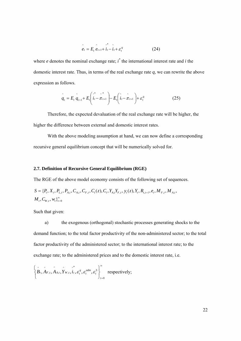
qtttttt iieEe ε+−+= +

^*^

1

^^ (24)

where e denotes the nominal exchange rate; i* the international interest rate and i the

domestic interest rate. Thus, in terms of the real exchange rate q, we can rewrite the above

expression as follows.

qtttttttttt iEiEqEq εππ +⎟

⎠⎞

⎜⎝⎛ −−⎟⎟

⎠

⎞⎜⎜⎝

⎛−+= +++ 1

^^*

1

^*^

1

^^ (25)

Therefore, the expected devaluation of the real exchange rate will be higher, the

higher the difference between external and domestic interest rates.

With the above modeling assumption at hand, we can now define a corresponding

recursive general equilibrium concept that will be numerically solved for.

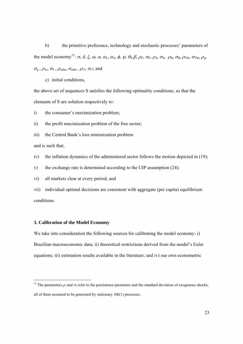
2.7. Definition of Recursive General Equilibrium (RGE)

The RGE of the above model economy consists of the following set of sequences.

∞=

+=

0,

,,1,,,,,,,

},,

,,,,,),(,,),(,,,,,,{

tttWt

tAtFttttttFtAtttFtAtAtLtt

wCM

MMeRYzyYYCzCCCPPXPS

Such that given:

a) the exogenous (orthogonal) stochastic processes generating shocks to the

demand function; to the total factor productivity of the non-administered sector; to the total

factor productivity of the administered sector; to the international interest rate; to the

exchange rate; to the administered prices and to the domestic interest rate, i.e.

∞

=⎭⎬⎫

⎩⎨⎧

0

*^

,

^

,

^

,

^^,,,,,,,

t

St

admt

qtttWtAtFt iYAAB εεε respectively;

23

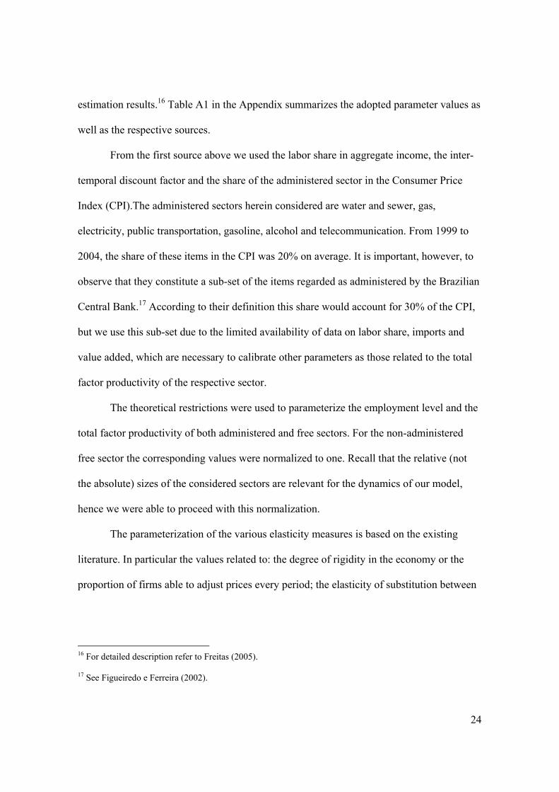
b) the primitive preference, technology and stochastic processes’ parameters of

the model economy15: σ, δ, ξ, ω, α, αL, αA, φ, ψ, θF,β, ρF, σF, ρA, σA, ρB, σB, ρYW, σYW, ρq,

σq , ρS,, σS , ρadm, σadm , ρi*, σi*; and

c) initial conditions,

the above set of sequences S satisfies the following optimality conditions, so that the

elements of S are solution respectively to:

i) the consumer’s maximization problem;

ii) the profit maximization problem of the free sector;

iii) the Central Bank’s loss minimization problem

and is such that,

iv) the inflation dynamics of the administered sector follows the motion depicted in (19);

v) the exchange rate is determined according to the UIP assumption (24);

vi) all markets clear at every period; and

vii) individual optimal decisions are consistent with aggregate (per capita) equilibrium

conditions.

3. Calibration of the Model Economy

We take into consideration the following sources for calibrating the model economy: i)

Brazilian macroeconomic data; ii) theoretical restrictions derived from the model’s Euler

equations; iii) estimation results available in the literature; and iv) our own econometric

15 The parameters ρi and σi refer to the persistence parameter and the standard deviation of exogenous shocks,

all of them assumed to be generated by stationary AR(1) processes.

24

estimation results.16 Table A1 in the Appendix summarizes the adopted parameter values as

well as the respective sources.

From the first source above we used the labor share in aggregate income, the inter-

temporal discount factor and the share of the administered sector in the Consumer Price

Index (CPI).The administered sectors herein considered are water and sewer, gas,

electricity, public transportation, gasoline, alcohol and telecommunication. From 1999 to

2004, the share of these items in the CPI was 20% on average. It is important, however, to

observe that they constitute a sub-set of the items regarded as administered by the Brazilian

Central Bank.17 According to their definition this share would account for 30% of the CPI,

but we use this sub-set due to the limited availability of data on labor share, imports and

value added, which are necessary to calibrate other parameters as those related to the total

factor productivity of the respective sector.

The theoretical restrictions were used to parameterize the employment level and the

total factor productivity of both administered and free sectors. For the non-administered

free sector the corresponding values were normalized to one. Recall that the relative (not

the absolute) sizes of the considered sectors are relevant for the dynamics of our model,

hence we were able to proceed with this normalization.

The parameterization of the various elasticity measures is based on the existing

literature. In particular the values related to: the degree of rigidity in the economy or the

proportion of firms able to adjust prices every period; the elasticity of substitution between

16 For detailed description refer to Freitas (2005).

17 See Figueiredo e Ferreira (2002).

25

differentiated goods; the export elasticity to the real exchange rate; the (inverse of) inter-

temporal elasticity of substitution; and to the (inverse of) the labor elasticity.

The remaining parameters regarding the degree of persistence and the variance of

the exogenous shocks were econometrically estimated as AR(1) processes. We also

estimated the parameters of the price determination equation of the administered sector.

Finally, sensitivity analysis was performed of the adopted parameterization. First

the parameterization above was taken as the benchmark case simulating the upper and

lower limits of the 95% confidence interval.18 Then, each parameter value was altered,

ceteris paribus, checking whether this alteration caused a statistically significant change in

the newly generated series. The results show that the model is robust for a rather wide

range of parameter values and that the derived standard deviation is very close to the one

found for the benchmark economy.

3.2. Reduced Form Equations

In order to fully characterize the benchmark economy in its reduced form, we next

introduce the set of reduced form equations of our model economy, namely the ones related

to the monetary authority’s utility function, the Phillips curve for the non-administered

sector, the price determination equation for the administered sector and the aggregated

demand function.

Taking into account the above parameterization of the benchmark economy, the

utility function of the monetary authority can be expressed as:

18 For each simulation 500 exogenous shocks were generated. For the computation of the standard deviation

the first 50 observations were dropped out.

26

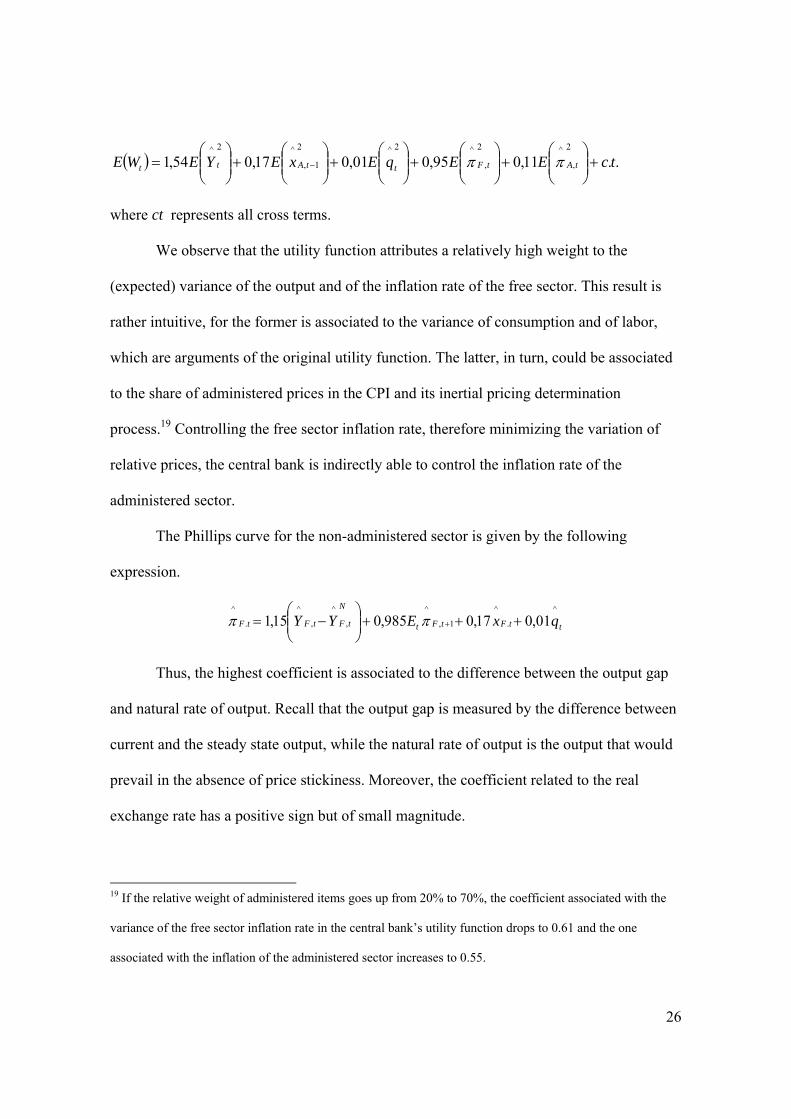
( ) ..11,095,001,017,054,12

,

^2

,

^2^2

1,

^2^tcEEqExEYEWE tAtFttAtt +⎟⎟

⎠

⎞⎜⎜⎝

⎛+⎟⎟

⎠

⎞⎜⎜⎝

⎛+⎟⎟

⎠

⎞⎜⎜⎝

⎛+⎟⎟

⎠

⎞⎜⎜⎝

⎛+⎟⎟

⎠

⎞⎜⎜⎝

⎛= − ππ

where ct represents all cross terms.

We observe that the utility function attributes a relatively high weight to the

(expected) variance of the output and of the inflation rate of the free sector. This result is

rather intuitive, for the former is associated to the variance of consumption and of labor,

which are arguments of the original utility function. The latter, in turn, could be associated

to the share of administered prices in the CPI and its inertial pricing determination

process.19 Controlling the free sector inflation rate, therefore minimizing the variation of

relative prices, the central bank is indirectly able to control the inflation rate of the

administered sector.

The Phillips curve for the non-administered sector is given by the following

expression.

ttFtFt

N

tFtFtF qxEYY^

.

^

1,

^

,

^

,

^

.

^01,017,0985,015,1 +++⎟⎟

⎠

⎞⎜⎜⎝

⎛−= +ππ

Thus, the highest coefficient is associated to the difference between the output gap

and natural rate of output. Recall that the output gap is measured by the difference between

current and the steady state output, while the natural rate of output is the output that would

prevail in the absence of price stickiness. Moreover, the coefficient related to the real

exchange rate has a positive sign but of small magnitude.

19 If the relative weight of administered items goes up from 20% to 70%, the coefficient associated with the

variance of the free sector inflation rate in the central bank’s utility function drops to 0.61 and the one

associated with the inflation of the administered sector increases to 0.55.

27

The corresponding reduced form for the administered sector price formation

equation is equivalent to its structural form, i.e.

admttAtttA xe εππ +−⎟

⎠⎞

⎜⎝⎛ ∆+= −−− 1,

^

1

^

1

^

,

^20,010,090,080,0

Finally, the aggregate demand reduced form equation or IS equation is given by:

tWtttttttttttt YqqEBEREYEY ,^^

1

^^

1

^1,

^1

^^03,014,037,0 +⎟

⎠⎞

⎜⎝⎛ −−⎥⎦

⎤⎢⎣⎡ −−−= ++++ π

With this parameterization of our model economy we proceed to numerically solve

for the RGE defined in Sub-section 2.7. The algorithm implemented in our computation is

based on Soderlind (1999), who suggests a generalization of the Schur decomposition to

deal with the unstable roots associated to the forward looking variables of the model

economy.20 This computation allows us to derive the artificially generated series, which

are presented and analyzed along the next section.

4. Main Simulation Results

This section presents the main results obtained from our numerical simulation. First, we

compare the standard deviation derived from the data with the one generated from our

model economy for selected main variables. The simulations show that the artificial

economy is able to fairly well mimic the empirically observed volatilities. Second, we

analyze the impulse responses of selected variables to exogenous nominal shocks and to

productivity shocks also in terms of their percentage deviation from the respective steady

state values. The evaluation of the impulse responses indicates the importance of

introducing the administered sector into the model economy, which allows us to derive a

20 The MatLab code is available upon request to the authors.

28

particular relative price adjustment process. Finally, we compute the utility level associated

to the achievement of the above theoretical micro-founded utility function, so-called the

central planer utility level (UCP). Then, we compare it to the one derived from an alternative

utility function specification, (UCB), in which a monetary authority is only concerned with

the minimization of the inflation variance. The obtained results are consistent with the

observed practice of inflation targeting regimes which take an headline price index (as

opposed to a core price index) as the target.

4.1. Standard Deviation Evaluation of the Benchmark Economy

This sub-section presents the simulation results, comparing the empirically observed series

with the artificially generated ones in terms of their volatility. We focused our analysis into

the inflation rates of the free sector and of the administered sector, the real exchange rate,

the nominal interest rate and the output gap. The data for the latter is extracted from a linear

trend of the natural logarithm of quarterly Brazilian GDP at market prices, computed by the

IBGE21, for the period 1994:3 to 2004:2. All series are taken as deviations (in logarithms)

from the respective sample mean value. Table 1 below summarizes the obtained results.

[Table 1 Here]

The first two lines of the above table present the standard deviation of the observed

series from the real economy for two different sample periods. The first one begins with the

implementation of the Real Plan (1994:3), and the second period starts with the floating

exchange rate regime (1999:1). The standard deviations of the artificial series on real

21 Brazilian Institute of Geography and Statistics.

29

exchange rate and on administered sector inflation rate are compared to the corresponding

statistics for the second sample period. This choice reflects the alteration of the prevailing

exchange rate regime and also the privatization program undertaken in the Country, which

made the administered pricing dynamics more predictable. On the other side, the

comparison of the artificial series corresponding to the free sector inflation rate, the output

gap and the short term nominal interest rate are based on the first sample period beginning

with the Real Plan22. Obviously, based on the Lucas’ critique, the implementation of the

inflation targeting regime in 1999 must have affected the above volatilities behavior.

Nonetheless, based on the arguments of the statistical advantage of using a larger sample

and the parameterization procedure adopted above, we kept the analysis using the first

sample period.

As shown in the above table, both artificially derived and observed standard

deviations are very close to each other. Only for the real exchange rate, the artificially

generated series shows a much smaller volatility than the data. One plausible explanation

can be the sample period used in the simulation: the exchange rate shock was modeled by

means of the residual of a VAR model, estimated from a sample period which includes the

Real Plan with a remarkable policy driven low volatility of the nominal exchange rate from

1994:3 to 1999:1.

The last five lines reports the results obtained taking into consideration one type of

exogenous shock at a time. We can conclude that the volatility of the administered sector

inflation rate can be mostly explained by the shock to the related pricing rule. Moreover,

22 We also compared the correlation coefficient of the artificial economy’s with the empirically observed

variables. The results were also satisfactory.

30

we can observe that this shock has also a strong impact on the volatilities of both the free

sector inflation rate and the nominal interest rate. Hence, it is apparent that the existence of

administered prices in an economy generates a new challenge for the conduction of

monetary policy, in particular for the inflation targeting regime.

Furthermore, we can observe that the volatility of the output gap can be mostly

explained by the productivity shock of the free (non-administered sector).23 However, the

results depend on the adopted parameterization. In particular, on the weight given to the

non-administered sector in the CPI captured by the parameter δ. For instance, if we take δ=

20%, instead of 80% as in the benchmark case, the exogenous shocks to the exchange rate,

to the demand or to the foreign interest rate become more relevant for explaining the

volatility of the output gap.

We can also infer that the second moment of the exchange rate series derived from

our model economy can be concurrently explained by the different considered shocks,

namely the ones to the free sector productivity, to the exchange rate and to the external

interest rate. Also these exogenous shocks are the ones relevant to explain the volatility of

the interest rate.24

4.2 Impulse Responses to Exogenous Shocks

23 Although this is a typical supply sock, this result does not lead to the conclusion that the monetary policy is

innocuous because it is in fact derived from the optimal response of the monetary policy to exogenous shocks.

24 Simulations considering shocks to demand, foreign income and administered sector’s productivity indicate

that they contribute only marginally to the volatilities of the above considered variables.

31

This section describes the impulse responses of key variables, namely the headline inflation

rate, the inflation rates of each sector (free and administered), the output gap, the interest

rate and the nominal as well as the real exchange rates, to exogenous shocks to

administered prices and to productivity.25 The respective values are in terms of percentage

deviation from their respective steady state values. Moreover, from the stationary property

of our model, the real exchange rate always returns to its long run equilibrium value.

Hence, since we are assuming that foreign prices are constant, the nominal exchange rate in

the long run can be interpreted as an accumulated variation of the price level, for the

variation of the nominal exchange rate has necessarily to reflect the variation of the

aggregate price index to attain the long run equilibrium real exchange rate.

4.2.1 Impulse-Response to a Shock to Administered Prices

Graphs 1a and 1b below are introduced in order to analyze the impacts of a shock to

administered prices. Graph 1a depicts the impulse-responses of the free sector inflation rate,

the aggregate inflation, the interest rate and the inflation rate of the administered sector.

Whereas Graph 1b shows in turn the impulse responses of the output gap, the nominal and

real exchange rate and the interest rate.

[Graph 1a and Graph 1b Here]

25 Impulse-responses to shocks to foreign as well as to domestic demand, interest rate and exchange rate were

also computed. They all presented very intuitive dynamics and are available from the authors under request.

32

In this case, we can infer the monetary policy effect of increasing the nominal

interest rate in order to partially off-set the inflationary pressure. Given a shock of 1 p.p. on

administered prices, the adaptative behavior of the central bank leads to an aggregate

inflation of about 0.35 percentage point. Hence, there is a strong movement in relative

prices. The administered goods become more expensive and consequently its demand falls

and, in turn, the equilibrium condition requires the reduction of the output of this sector. On

the other hand, even with an increase of the real interest rate of approximately 0.03 p.p.,

demand and, hence, output in the free prices sector increase due to the fall in its relative

price. Thus, the aggregate output gap falls about 8% as shown it Graph 1b, resulting from a

reduction of 70%26 in the output gap of the administered sector and an increase of 5% in

the output gap of the free sector.

This shock has also a significant impact on the new equilibrium price level of about

1.1 times the magnitude of the original shock. Besides this direct impact on the aggregate

inflation rate, the higher relative price of administered items induces a higher consumption

of free goods, which completely offsets the depressing effect of a higher real interest rate

on demand.

On the other side, the higher output gap of the free sector brought about by this

relative price effect, induces a higher inflation rate in this sector, which in turn feeds the

next period (higher) inflation rate of administered prices.

In period t+2, the monetary authority would again accommodate the above

inflationary pressure, allowing for a new round of (higher) administered inflation rate in

26 The percentage values are approximations, for they are the difference in logarithms from the steady state

values. Hence, the smaller the deviation the more accurate this approximation.

33

t+3, and so forth. Therefore, even though the shock to administered prices is not auto-

correlated, the dynamic path of the free price inflation rate becomes much more persistent

than those observed for other low auto-correlated shocks.

The final impact on the price level will be stronger the weaker the adjustment

mechanism of administered prices to the long run equilibrium relative price, which in our

model is normalized to one. According to the parameterization adopted above, our

simulation shows that approximately 20% of the previous period observed deviation of

relative prices is corrected along the re-adjustment process of administered prices in our

model economy. If, for instance, we take instead a correction factor of 5%, the long run

equilibrium price level reaches approximately 5 times the value of the initial shock.

From a normative point of view, the above simulation results suggest that the

monetary authority should not keep the aggregate inflation close to zero by means of a

deflation in the free sector in order to neutralize the inflationary pressure of administered

prices. This policy could even be economically unfeasible, for the deflation of free prices

could lead to a higher demand and a lower supply in this sector, hence, generating

disequilibrium in the goods market.

Finally, we can observe that the free sector inflation rate is higher the higher the

weight of administered items into the economy. In order to illustrate this point, Graph 2

below compares the reaction of the free sector inflation rate to a shock in administered

prices for two economies. For the first one we consider a weight of administered items in

the CPI of 20%, depicted by a solid line and, for the second case we increase this weight to

80% with responses depicted in dashed lines. As it can be seen, the higher the weight of

administered items in the CPI, the higher the free sector inflation rate allowed by the central

34

bank in order to smooth the relative price changes. Thus, this accommodating policy avoids

a sharper decline in aggregate output.

[Graph 2 Here]

4.2.2 Impulse-responses to a Productivity Shock in the Free Sector

The simulation results in this case are quite intuitive as can be seen in Graphs 3a and 3b

below. Our objective is to contrast these results with the less intuitive ones obtained in the

case of a productivity shock to the administered sector.

[Graph 3a and Graph 3b Here]

As expected, in this case, the interest rate falls contemporaneously to the realization

of the shock as shown in Graph 3a, stimulating a higher output gap (Graph 3b) and, hence,

internalizing the productivity gains of the free sector. We can also see that a productivity

shock in the free sector leads to a deflation in this sector as depicted in Graph 3a, even

though there is a fall in the interest rate and an increase in output (Graph 3b). Moreover,

this deflationary impact through the productivity gain is attenuated due to the exchange rate

devaluation brought about by a lower real interest rate (Graph 3b). In our model economy

where the UIP holds, we can see in Graph 3a that the deflation of free prices reaches 10%

in t=1 and, in the long run, the price level settles to a lower lever than the original one.

35

4.2.3 Impulse Responses to a Productivity Shock in the Administered Sector

Graphs 4a and 4b below show, in turn, the impulses responses generated by a productivity

shock in the administered sector. This productivity gain leads to an increase in the output

gap. Nevertheless, contrary to the results obtained above from a productivity shock in the

free sector, this shock also brings about an inflationary pressure of above 3.5% due to the

pricing equation assumed for this sector in our model economy.

As expected, this shock stimulates more strongly the production in the administered

sector. Thus, we can observe in Graph 4b that in t=1 the output gap increases more than

1.25 percent points.

[Graph 4a and Graph 4b Here]

In order to attain a higher output in the administered sector than in the free sector,

the market equilibrium condition requires the increase in the consumption of the former to

be higher than the increase in the consumption of the latter. Hence, it is necessary to have a

lower relative price of administered goods. Nevertheless, without any exogenous shock that

can directly affect its price, administered prices can only increase through inflation or

exchange rate devaluation in the previous period, which is not the case in t=1. Thus, as can

be seen in Graph 4a the reduction of the relative price of administered goods is only

possible through an inflationary pressure of the free sector.

This inflationary pressure in turn leads the central bank to increase the nominal

interest rate, but less than the expected inflation. For by means of a (policy driven) lower

real interest rate, the economy can attain a higher output gap brought about by the

productivity gain.

36

4.3 Evaluation of Alternative Utility Functions

The aim of this sub-section is to discuss the type of price index that the monetary authority

should adopt as the policy target, based on a social welfare point of view.

The objective function of the central bank was derived from the economy’s micro-

foundations. Its arguments included the second moments of the output gap, the inflation

rate, the exchange rate and the relative prices, along with the co-variances amongst these

variables and amongst them and the exogenous shocks included in the model economy.

Nevertheless, in an inflation targeting regime, the monetary authority receives the

incumbency of guaranteeing that the inflation rate could converge to a determined targeted

level. Hence, their real objective function could potentially differ from the one theoretically

derived above.

The international experience has shown that there is not a single case in which the

board of directors of a central bank is forced to attain a given inflation rate target regardless

of the associated social costs. There are, in fact, institutional arrangements that allows them

some flexibility, for example: the definition of a band or interval within which the inflation

rate is tolerated; establishment of escape clauses, i.e., a list of predefined shocks that

exempts the central bank from the obligation of reaching the target; and, as in the Brazilian

case, the possibility for the Governor of the Central Bank to issue a so-called Open Letter

to the Ministry of Finance explaining the reasons for failing to attain the targeted inflation.

These resources are important in order to allow central banks to pursue a monetary policy

as close as possible to the optimal one. Still, even in the context of more flexible

institutional arrangements, central banks do have to be especially concerned about inflation,

particularly when their credibility is weak.

37

Along this line of argument, naturally arises the (theoretical) question of the social

impact of having a monetary authority with an objective function which differs from the

one obtained in Sub-section 2.5, namely one whose only argument is the variance of the

inflation rate. To this end, we perform a simulation in which we assumed the central bank

chooses the short run nominal interest rate in order to minimize the variance of the inflation

rate around the targeted level.

This exercise in turn generates several sequences of the key macroeconomic

variables. Then, their corresponding second moments can be imputed back into the original

benchmark objective function derived in Sub-section 2.5. We denote this utility level as

UCB, where CB stands for central bank. Therefore, UCB is the welfare achieved when

monetary policy is conducted in order to maximize the utility of the central bank, i.e., the

one whose only argument is the variance of inflation.

Using the same exogenous shock sequences, we compute in turn the solution

associated to the original optimization problem. The second moments associated to the

sequences generated in this case allow us to compute the utility which is denoted by UCP,

named after the utility the economy would achieve in the presence of a central planner.

Observe that both above measures are expressed in utility units. Thus, the difference

(UCP – UCB), which is a measure of the utility loss for adopting the alternative objective

function, is sensitive to linear transformations of the objective function.

Nevertheless, we can compute the associated percentage loss, i.e. (UCB/UCP – 1),

and also the statistical discrepancy between the two measures. But, this percentage loss

measure has also to be taken cautiously. First, it is related to the percentage loss associated

to the monetary policy action and it does not reflect the total utility loss. Following the

suggestions of the available literature, we neglected the terms which do not depend on the

38

monetary policy (TIPM), as those related to the second moments of the exogenous

shocks.27 Second, this measure is sensitive to linear transformations of the utility function.

In particular, we would get the same set of solutions solving the maximization problem

using the return function F1 = U(.) or F2 = U(.) + K, where K denotes an arbitrary constant.

But the percentage loss associated to the latter is given by L% = (UCB – UCP)/(U(.)CP+K).

Hence, if the arbitrary constant approaches -UCP the percentage loss would tend to infinity.

On the other hand, regarding the statistical difference between UCB and UCP, we

conducted a conventional statistical test. First, a distribution of the utility derived from UCP

was generated28. Then, we computed the utility level using the alternative objective

function and located this utility level in the UCP distribution. From this information and

using a pre-determined level of statistical significance we tested H0: UCB = UCP against H1:

UCB < UCP.

It is still necessary to define which inflation index the central bank will target, the

headline index or a core one The computation of the alternative utility level – UCB – was

undertaken for different inflation indexes. These indexes were in turn calculated based on

linear combination of inflations in the free sector and in the administered price sector, with

weights ranging from 0% to 100%, with a 10% increment. Thus, eleven price indexes were

used to compute UCB, and for each one we could quantitatively asses two measures of

welfare-loss. The first one is the difference between UCB for the corresponding price index

27 In order to derive the percentage loss in terms of the aggregated utility level we would need to sum up the

TIPM to the obtained utility measure, which in turn would alter the percentage loss measure, except when

TIPM=0.

28 This distribution was generated from 500 series for each shock, each one with 500 observations. The

computations of the second moments were performed using the values starting from the 50th realization.

39

and UCP. The second loss is obtained by comparing the welfare associated with the price

index that leads to maximum UCB. Table 2 below shows the two measures of welfare loss

associated with each price index when the economy is hit by all shocks and the associated

losses when the economy is hit by a specific shock.

[Table 2 Here]

The first column of the table above shows the first measure of welfare loss, i.e., the

percentage loss associated to the adoption of the alternative utility function with respect to

the theoretically correct specification. Therefore, if the central bank cares sorely on the

volatility of the inflation rate, using a price index with 20% of administered prices; there is

an 18% loss, which is not statistically different from zero. Thus, from the statistical point of

view, the economy we are analyzing does not have any welfare loss if the monetary

authority takes into consideration only the variance of the inflation rate, instead of trying to

maximize the social utility function derived in section 2.5. Observe that this result holds

for the whole range of price indexes, but for those indexes with a weight of administered

items above 90%.

The percentage loss measures of the second column were normalized with respect to

the price index that maximizes the alternative utility function, which is the one with a

weight of administered prices of 10%. Hence, from a social welfare point of view, our

simulation results do not support the adoption of a core inflation index which excludes the

administered items,. Moreover, the adoption of the headline index as the target is associated

to a mild loss of 0.7% with respect to the adoption of the welfare maximizing index, and to

a loss of 0.6% with respect to the adoption of an ex-administered price goods core index.

40

The last four columns of the above Table 2 show in turn the percentage loss

normalized with respect to the welfare maximizing index assuming that only one

exogenous shock hits the model economy at a time. We can infer that the choice of the

price index that maximizes UCB depends on the considered shock. For instance, if the

central bank believes that the shocks to the exchange rate are the relevant ones, there is a

positive argument supporting the use of a core inflation index as the target, for the

percentage loss associated to the use of the headline inflation index as the target reaches

49%. On the other side, in case the shocks to the administered prices are the relevant ones,

the targeted inflation index should attribute a higher weight – of 80% – to the administered

items, instead of the weight of 20% observed in the real economy. In this case the

utilization of a core inflation index would lead to a loss of approximately 14.6% - 8.2% =

6%.

Therefore, the results obtained above are consistent with the common observe

practice of adopting an headline price index as the target29, for the welfare loss associated

with its utilization appears to be low and not statistically significant.30

Nevertheless, even assuming UCB = UCP, the associated expected loss of 18.5%

associated to the utilization of the headline CPI as the target is relatively high. Thus, this

result is differs from the one presented by Aoki (2001), King and Wolman (1999) and

Woodford (2003), who suggest that the central bank should minimize only the variance of a

determined price index. Once again, this discrepancy could be a result of the particular set

29 See Schmidt-Hebel and Tapia (2002) ans also Ferreira and Petrassi (2002).

30 Observe that our model does not consider either the cost in terms of transparency and credibility associated

to the use of a core index by the monetary authority.

41

up adopted for our model economy with two distinct productive sectors and imported

production inputs.

Conclusion

The present study aimed to quantitatively evaluate the inclusion of administered prices for

the conduct of monetary policy, in particular for an inflation targeting regime. To this end,

we suggest a (short run) recursive general equilibrium model for a small open economy.

In spite of the inherent limitations of any artificial economy and the problems

associated to the quality of the available Brazilian time series data, the model generated

sequences of the main macroeconomic variables, namely the output gap, the inflation rates

of free and administered prices, the real exchange rate and the nominal interest rate, with

corresponding second moments very close to the ones observed in the data.

We have seen that the response of the free price inflation rate to the exogenous

shocks depends on the degree of accommodation desired by the monetary authority.

Generally speaking, we observe that the central bank would optimally accommodate the

shocks not only in the short run, but should also allow permanent price level changes in the

long run. Thus, the central bank should not stabilize the free sector prices, contrary to the

suggestions given by Clarida, Gali and Gertler (1999) for a demand shock, King and

Wolman (1999) for a productivity shock, Woodford (2003) and Aoki (2001) for both

demand and supply shocks. The reason behind this result lies on the characterization of our

model economy, using two sectors with different technologies. Intuitively speaking, if both

sectors were technologically equal, the central bank could set the nominal interest rate to

the natural level, such that the resulting inflation rate would be zero. Otherwise, when the

sectors are different, the changes in the respective potential output also differ as well as the

42

natural interest rate. Since the monetary authority controls only one interest rate, the fine

tuning of the interest rate in order to equalize the interest the natural rate in both sectors

becomes more difficult.

Furthermore, the rigidity of the administered pricing rule is important to explain the

free prices inflation rate response to shocks to the productivity and to the prices of the

administered sector.. One would expect that positive productivity shocks would be

deflationary for the affected sector. Nevertheless, due to the rigidity of administered prices,

the corresponding relative price adjustment is undertaken through inflationary responses in

the free sector.

On the other hand, the impulse responses resulting from an exogenous shock to

administered prices show that the monetary authority should conduct its policy allowing for

some inflationary pressure in the free sector. This accommodation must be higher the

higher the weight of administered items into the consumption bundle, in order to partially

neutralize the relative price changes caused by the shock.

Therefore, our results allow us to get more insights than the obtained ones from a

one sector model. For the higher expected inflation could be achieved through a higher

inflation rate of administered prices and deflation or price stability in the free sector, or

with inflation for both sectors.

Welfare simulation results did not support the adoption of a core inflation index that

excludes administered prices as the monetary policy target. Moreover, the price index that

maximizes social welfare depends on the type of shock the economy is facing. For instance,

under a shock to administered prices, the utilization of a headline consumer price index as

monetary target would lead the model economy to a higher welfare, compared to the

welfare achieved when an ex-administered price-goods core index is adopted as the target.

43

As any model economy, the one built up for the present study is a useful

simplification of the reality. Futures extension of this research could incorporate an

endogenous investment decision and capital formation such that we could analyze the long

run behavior of the economy. Another extension would be to introduce a government into

the model, for the introduction of administered prices affect the optimal response of interest

rates and, within a fiscal dominance framework, if the government is a highly debtor agent

in the economy, those prices would indeed affect the optimal monetary response.

Finally, the present study did not considered issues on the credibility of the inflation

targeting regime. This question becomes a relevant problem in face of cost-push shocks,

like shocks to productivity, to the exchange rate, to foreign interest rate and to administered

prices. We have shown in the latter case, that the higher the weight of administered items,

the higher the inflationary pressure. The optimal response of the central bank may turn up

to be not so accommodative if such inflationary pressures can threat the credibility of the

inflation targeting regime.

44

Appendix

Table A1 - Summary of Calibrated Parameters

Parameter Value Source

Parameterization based on observed aggregated data

δ (weight of free goods into the GPI) 0.8 GPI, IBGEα A (labor income share, administered sector) 0.7 National Account Statistics, IBGE α L (labor income share, free sector) 0.85 National Account Statistics, IBGE β (inter-temporal discount factor) 0.985 Historic data on real interest rate (Selic – GPI)

A L (total factor productivity, free sector) 1 normalized A A (total factor productivity, administered sector) 0.44N A (employment level, administered sector) 0.54N L (employment level, free sector) 1 normalized

Parameterization Based on the Available Literature α (degree of rigidity) 0.25 Naish (1994)ξ (elasticity of substitution differenciated goods) 4 Parrado (2004) and Gironni e Rebucci (2001)θ F

(export elasticity to the real exchange rate) 0.8 Faini et al (1999)σ (inverse of the inter-temporal elasticity of substitution) 2.25 Araujo and Issler(2004) φ (inverse of the elasticity of labor supply to the real wage) 0.5 Fernandes et al (2004) Estimated Parameters Shock to External Interest Rate ρ i* (auto-regressive coefficient) 0.9

σ i* (standard deviation) 0.003Shock to External Income ρ Yf (auto-regressive coefficient) 0.8

σ Yf (standard deviation) 0,004Shock to Demand ρ B (auto-regressive coefficient ) 0.34 σ B (standard deviation) 0.15Shock to Interest Rate ρ i (auto-regressive coefficient) 0.24

σ i (standard deviation) 0.116Shock to Exchange Rate ρ c (auto-regressive coefficient) 0.2

σ c (standard deviation) 0.06Shock to Administered Prices ρ a (auto-regressive coefficient) 0

σ a (standard deviation) 0.03Productivity Shock, Free Sector

ρ AL (auto-regressive coefficient) 0.7

σ AL (standard deviation) 0.03Productivity Shock, Administered Sector ρ AA (auto-regressive coefficient) 0.8

σ AA (standard deviation) 0.04Coefficients of Administered Prices Determination Rule ψ (adjustment coefficient of relative prices) 0.8 ω (adjustment coefficient of past inflation) 0.9

45

Bibliographical References

Amato, J. & Laubach, T. (2003). Rule of thumb behavior and monetary policy. European

Economic Review, 47, 5, 791-831.

Aoki, K. (2001). Optimal monetary policy responses to relative price changes. Journal of

Monetary Economics, 48, 1, 55-80.

Araujo, F. & Issler, J. V. (2004). Identificação do fator estocástico de descontos e algumas

implicações sobre testes de modelos de consumo. Trabalhos para Discussão do Banco

Central do Brasil, 86.

Calvo, G. (1983). Staggered prices in a utility-maximizing framework. Journal of Monetary

Economics, 12, 383-398.

Clarida, R., Gali, J. & Gertler, M. (1999). The science of monetary policy: a new

Keynesian perspective. Journal of Economic Literature, 37, 1661-1707.

___________________________________ (2001). Optimal monetary policy in closed

versus open economies. NBER Working Paper, 8604.

Dixit, A. & Stiglitz, J. (1977). Monopolistic competition and optimum product diversity.

American Economic Review, 67, 297-308.

Faini, R., Pritchett, L., Clavijo, F., Dagenais, M.G. & Muet, P. A (Eds) (1992). Import

Demand in Developing Countries. London: Chipman and Hall.

Fernandes, R., Gremaud, Amaury P. & Narita, R. T. (2004). Estrutura tributária e

formalização da economia: simulando diferentes alternativas para o Brasil. Anais do XXV!

Encontro Brasileiro de Econometria, João Pessoa, PB, Brasil.

Ferreira, T. & Petrassi, M. (2002). Regime de metas para a inflação: resenha sobre a

experiência internacional. Notas Técnicas do Banco Central do Brasil, 30.

46

Figueiredo, F. & Ferreira, T. (2002). Os preços administrados e a inflação no Brasil.

Trabalhos para Discussão do Banco Central do Brasil, 59.

Freitas, P. S. de. (2005). Preços Administrados e Política Monetária. PhD Dissertation,

Dept of Economics, Universidade de Brasília.

Ghioroni, F. & Rebucci, A. (2001). Monetary Rules for Emerging Market Economie,

Mimeo.

King, R. & Wolman, A. L. (1999). What should the monetary authority do when prices are

sticky?. In J. B. Taylor (Ed.), Monetary Policy Rules (pp. 349-398). Chicago: University of

Chicago Press.

Mankiw, N. G. & Reis, R. (2003). What measure of inflation should a central bank target?

Journal of the European Economic Association, 1, 5, 1058-1086.

Minella, A., Freitas, P., Goldfajn, I. & Muinhos, M. (2003). Inflation targeting in Brazil:

constructing credibility under exchange rate volatility. Journal of International Money and

Finance, 22, 7, 1015-1040.

Naish, H. F. (1994). On the infrequent adjustment of prices by firms. Economic Inquiry, 33,

4, 642-654.

Parrado, E. (2004). Inflation Targeting and Exchange Rate Rules in an Open Economy.

IMF Working Paper, 24.

Rotemberg, J. & Woodford, M. (1997). An optimization-based econometric framework for

the evaluation of monetary policy. In NBER Macroeconomics Annual (pp. 297-346).

Massachussetts: MIT Press.

Schmidt-Hebel, K. & Tapia, M. (2002). Monetary policy implementation and results in

twenty inflation targeting countries. Working Paper Central Bank of Chile, 166.

47

Soderlind, P. (1999). Solution and estimation of RE macromodels with optimal policy.

European Economic Review, 43, 4, 813-823.

Woodford, M. (2003). Interest and Prices: Foundations of a Theory of Monetary Policy.

Princeton: Princeton University Press.

48

Table 1 - Standard Deviations of Observed and Artificial Series

Standard Deviation

Adm-Sector

Inflation Rate

Real Exchange

Rate

Output Gap Free-Sector

Inflation Rate

Nominal Interest

Rate

Period Real Economy

1994:3 – 2004:2 0.030 0.304 0.024 0.024 0.027

1999:1 – 2004:2 0.026 0.150 0.017 0.013 0.010

Model Economy

Benchmark 0.0338 0.0833 0.0304 0.0173 0.0289

Productivity 0.0321 0.0731 0.0285 0.0138 0.0274

Exchange Rate 0.0324 0.0716 0.0206 0.0138 0.0421

Adm-Prices 0.0320 0.0619 0.0207 0.0131 0.0413

Nom. Int. Rate 0.0331 0.0632 0.0216 0.0161 0.0412

Ext. Int. Rate 0.0327 0.0783 0.0206 0.0151 0.0422

49

Table 2 - Percentage Loss in Utility by Alternative Price Index and Exogenous Shock

Exogenous Shocks

Weight of

Administered

Prices into GPI

Benchmark

Objective

Function

Maximizing

Price Index

Productivity

Free Sector

Exchange

Rate*

Administered

Prices*

Interest Rate

0.0 17.5 0.11 0.44 0.00 14.59 0.00

0.1 17.5 0.00 0.24 23.04 11.15 0.69

0.2 18.1 0.71 0.09 48.69 8.15 0.69

0.3 19.3 2.22 0.01 76.96 5.59 1.38

0.4 21.2 4.54 0.00 107.85 3.52 2.07

0.5 23.9 7.71 0.07 141.62 1.91 2.76

0.6 27.1 11.72 0.22 177.75 0.79 2.76

0.7 31.2 16.61 0.44 216.75 0.13 3.45

0.8 35.9 22.33 0.75 258.38 0.00 4.14

0.9 41.4** 28.99** 1.16 302.36 0.36 4.83

1.0 47.6** 36.51** 1.66 349.21 1.23 5.52

*All elements in the column are statistically significant at 5%; **statistically significant at 10%

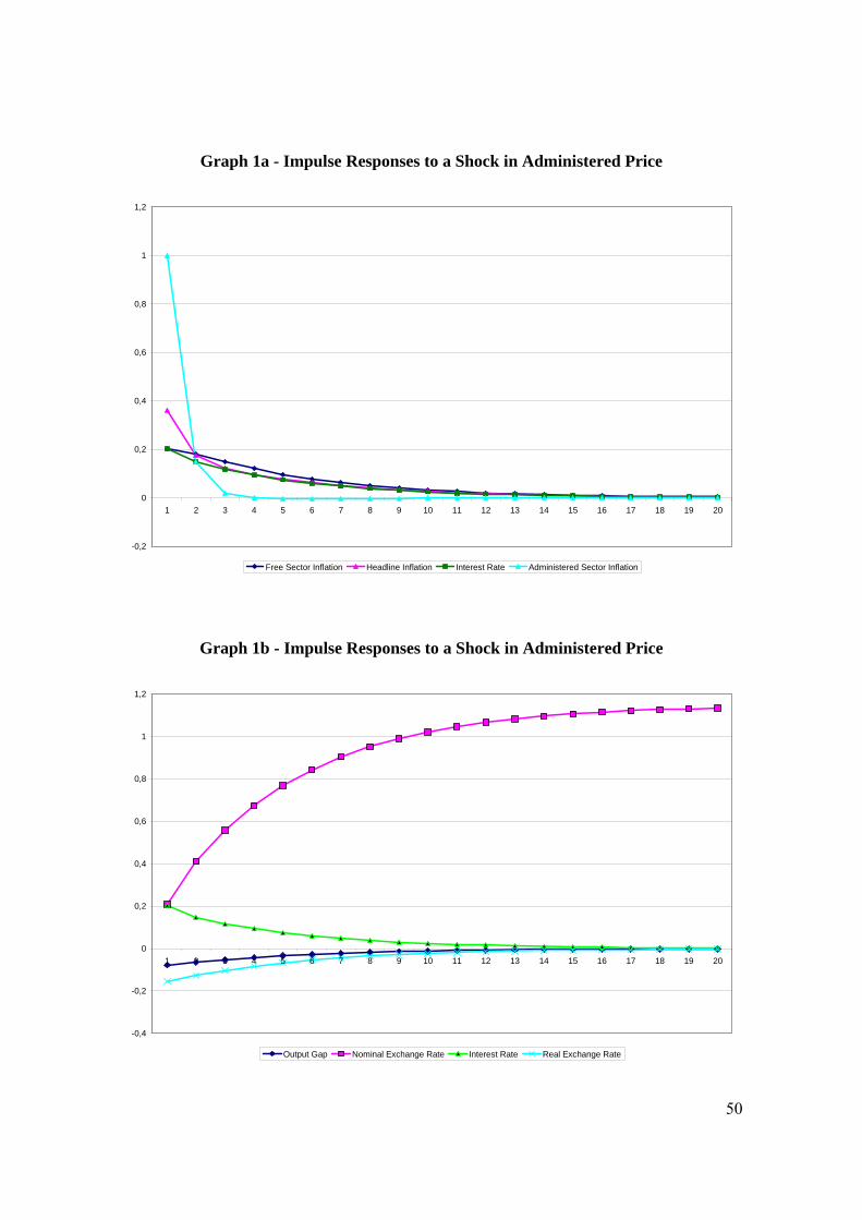
50

Graph 1a - Impulse Responses to a Shock in Administered Price

-0,2

0

0,2

0,4

0,6

0,8

1

1,2

1 2 3 4 5 6 7 8 9 10 11 12 13 14 15 16 17 18 19 20

Free Sector Inflation Headline Inflation Interest Rate Administered Sector Inflation

Graph 1b - Impulse Responses to a Shock in Administered Price

-0,4

-0,2

0

0,2

0,4

0,6

0,8

1

1,2

1 2 3 4 5 6 7 8 9 10 11 12 13 14 15 16 17 18 19 20

Output Gap Nominal Exchange Rate Interest Rate Real Exchange Rate

51

Graph 2 - Responses of the Free Sector Inflation Rate to a Shock on Administered

Prices with Different Weights in GPI

0.000

0.100

0.200

0.300

0.400

0.500

0.600

0.700

0.800

0.900

1 2 3 4 5 6 7 8 9 10 11 12 13 14 15 16 17 18 19 20

Weight of Adm Items = 20% Weight of Adm Items = 80%

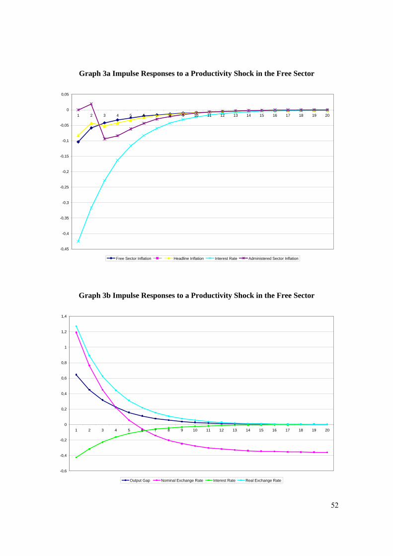
52

Graph 3a Impulse Responses to a Productivity Shock in the Free Sector

-0,45

-0,4

-0,35

-0,3

-0,25

-0,2

-0,15

-0,1

-0,05

0

0,05

1 2 3 4 5 6 7 8 9 10 11 12 13 14 15 16 17 18 19 20

Free Sector Inflation Headline Inflation Interest Rate Administered Sector Inflation

Graph 3b Impulse Responses to a Productivity Shock in the Free Sector

-0,6

-0,4

-0,2

0

0,2

0,4

0,6

0,8

1

1,2

1,4

1 2 3 4 5 6 7 8 9 10 11 12 13 14 15 16 17 18 19 20

Output Gap Nominal Exchange Rate Interest Rate Real Exchange Rate

53

Graph 4a Impulse Responses to a Productivity Shock in the Administered Sector

0

0,005

0,01

0,015

0,02

0,025

0,03

0,035

0,04

0,045

0,05

1 2 3 4 5 6 7 8 9 10 11 12 13 14 15 16 17 18 19 20

Free Sector Inflation Headline Inflation Interest Rate Administered Sector Inflation

Graph 4b Impulse Responses to a Productivity Shock in the Administered Sector

0

0,05

0,1

0,15

0,2

0,25

1 2 3 4 5 6 7 8 9 10 11 12 13 14 15 16 17 18 19 20

Output Gap Nominal Exchange Rate Interest Rate Real Exchange Rate