Semigroup Kernels on Measures

Journal of Machine Learning Research 6 (2005) 1169–1198 Submitted 1/05; Published 7/05

Semigroup Kernels on Measures

Marco Cuturi [email protected]

Ecole des Mines de Paris35 rue Saint Honore77305 Fontainebleau, France;Institute of Statistical Mathematics4-6-7 Minami-Azabu, Minato-Ku, Tokyo, Japan

Kenji Fukumizu FUKUMIZU @ISM.AC.JP

Institute of Statistical Mathematics4-6-7 Minami-Azabu, Minato-Ku, Tokyo, Japan

Jean-Philippe Vert [email protected]

Ecole des Mines de Paris35 rue Saint Honore77305 Fontainebleau, France

Editor: John Lafferty

Abstract

We present a family of positive definite kernels on measures,characterized by the fact that the valueof the kernel between two measures is a function of their sum.These kernels can be used to derivekernels on structured objects, such as images and texts, by representing these objects as sets ofcomponents, such as pixels or words, or more generally as measures on the space of components.Several kernels studied in this work make use of common quantities defined on measures suchas entropy or generalized variance to detect similarities.Given an a priori kernel on the spaceof components itself, the approach is further extended by restating the previous results in a moreefficient and flexible framework using the “kernel trick”. Finally, a constructive approach to suchpositive definite kernels through an integral representation theorem is proved, before presentingexperimental results on a benchmark experiment of handwritten digits classification to illustratethe validity of the approach.

Keywords: kernels on measures, semigroup theory, Jensen divergence,generalized variance,reproducing kernel Hilbert space

1. Introduction

The challenge of performing classification or regression tasks over complex and non vectorial ob-jects is an increasingly important problem in machine learning, motivated by diverse applicationssuch as bioinformatics or multimedia document processing. The kernel methodapproach to suchproblems (Scholkopf and Smola, 2002) is grounded on the choice of a proper similarity measure,namely a positive definite (p.d.) kernel defined between pairs of objects ofinterest, to be usedalongside with kernel methods such as support vector machines (Boser et al., 1992). While naturalsimilarities defined through dot-products and related distances are availablewhen the objects lie ina Hilbert space, there is no standard dot-product to compare strings, texts, videos, graphs or other

c©2005 Marco Cuturi, Kenji Fukumizu and Jean-Philippe Vert.

CUTURI, FUKUMIZU AND VERT

structured objects. This situation motivates the proposal of various kernels, either tuned and trainedto be efficient on specific applications or useful in more general cases.

One possible approach to kernel design for such complex objects consists in representing themby sets of basic components easier to manipulate, and designing kernels on such sets. Such basiccomponents can typically be subparts of the original complex objects, obtained by exhaustive enu-meration or random sampling. For example, a very common way to represent atext for applicationssuch as text classification and information retrieval is to break it into words and consider it as abag of words, that is, a finite set of weighted terms. Another possibility is to extract all fixed-lengthblocks of consecutive letters and represent the text by the vector of counts of all blocks (Leslie et al.,2002), or even to add to this representation additional blocks obtained by slight modifications of theblocks present in the text with different weighting schemes (Leslie et al., 2003). Similarly, a grey-level digitalized image can be considered as a finite set of points ofR

3 where each point(x,y, I)stands for the intensityI displayed on the pixel(x,y) in that image (Kondor and Jebara, 2003).

Once such a representation is obtained, different strategies have beenadopted to design kernelson these descriptions of complex objects. When the set of basic componentsis finite, this repre-sentation amounts to encode a complex object as a finite-dimensional vector ofcounters, and anykernel for vectors can be then translated to a kernel for complex objectthrough this feature represen-tation (Joachims, 2002, Leslie et al., 2002, 2003). For more general situations, several authors haveproposed to handle such weighted lists of points by first fitting a probability distribution to eachlist, and defining a kernel between the resulting distributions (Lafferty andLebanon, 2002, Jebaraet al., 2004, Kondor and Jebara, 2003, Hein and Bousquet, 2005). Alternatively, Cuturi and Vert(2005) use a parametric family of densities and a Bayesian framework to define a kernel for stringsbased on the mutual information between their sets of variable-length blocks,using the concept ofmutual information kernels (Seeger, 2002). Finally, Wolf and Shashua (2003) recently proposed aformulation rooted in kernel canonical correlation analysis (Bach and Jordan, 2002, Melzer et al.,2001, Akaho, 2001) which makes use of the principal angles between thesubspaces generated bythe two sets of points to be compared when considered in a feature space.

We explore in this contribution a different direction to kernel design for weighted lists of basiccomponents. Observing that such a list can be conveniently representedby a molecular measureon the set of basic components, that is a weighted sum of Dirac measures, or that the distributionof points might be fitted by a statistical model and result in a density on the same set, we formallyfocus our attention on the problem of defining a kernel between finite measures on the space of basiccomponents. More precisely, we explore the set of kernels between measures that can be expressedas a function of their sum, that is:

k(µ,µ′) = ϕ(µ+µ′). (1)

The rationale behind this formulation is that if two measures or sets of pointsµ andµ′ overlap, thenit is expected that the sumµ+ µ′ is more concentrated and less scattered than if they do not. As aresult, we typically expectϕ to quantify the dispersion of its argument, increasing when it is moreconcentrated. This setting is therefore a broad generalization of the observation by Cuturi and Vert(2005) that a valid kernel for strings, seen as bags of variable-lengthblocks, is obtained from thecompression rate of theconcatenationof the two strings by a particular compression algorithm.

The set of measures endowed with the addition is an Abelian semigroup, and the kernel (1)is exactly what Berg et al. (1984) call asemigroup kernel. The main contribution of this paperis to present several valid positive definite (p.d.) semigroup kernels for molecular measures or

1170

SEMIGROUPKERNELS ONMEASURES

densities. As expected, we prove that several functionsϕ that quantify the dispersion of measuresthrough their entropy or through their variance matrix result in valid p.d. kernels. Using entropy tocompare two measures is not a new idea (Rao, 1987) but it was recently restated within differentframeworks (Hein and Bousquet, 2005, Endres and Schindelin, 2003,Fuglede and Topsøe, 2004).We introduce entropy in this paper slightly differently, noting that it is a semigroup negative definitefunction defined on measures. On the other hand, the use of generalizedvariance to derive a positivedefinite kernel between measures as proposed here is new to our knowledge. We further show howsuch kernels can be applied to molecular measures through regularization operations. In the case ofthe kernel based on the spectrum of the variance matrix, we show how it can be applied implicitlyfor molecular measures mapped to a reproducing kernel Hilbert space when a p.d. kernel on thespace of basic components is provided, thanks to an application of the “kernel trick”.

Besides these examples of practical relevance, we also consider the question of characterizingall functionsϕ that lead to a p.d. kernel through (1). Using the general theory of semigroup kernelswe state an integral representation of such kernels and study the semicharacters involved in thisrepresentation. This new result provides a constructive characterization of such kernels, which webriefly explore by showing that Bayesian mixtures over exponential modelscan be seen as naturalfunctionsϕ that lead to p.d. kernels, thus making the link with the particular case treated by Cuturiand Vert (2005).

This paper is organized as follows. We first introduce elements of measurerepresentations ofweighted lists and define the semigroup formalism and the notion of semigroup p.d. kernel in Sec-tion 2. Section 3 contains two examples of semigroup p.d. kernels, which are however usuallynot defined for molecular measures: the entropy kernel and the inversegeneralized variance (IGV)kernel. Through regularization procedures, practical applications ofsuch kernels on molecular mea-sures are proposed in Section 4, and the approach is further extendedby kernelizing the IGV throughan a priori kernel defined itself on the space of components in Section 5. Section 6 contains the gen-eral integral representation of semigroup kernels and Section 7 makes thelink between p.d. kernelsand Bayesian posterior mixture probabilities. Finally, Section 8 contains an empirical evaluation ofthe proposed kernels on a benchmark experiment of handwritten digits classification.

2. Notations and Framework: Semigroup Kernels on Measures

In this section we set up the framework and notations of this paper, in particular the idea of semi-group kernel on the semigroup of measures.

2.1 Measures on Basic Components

We model the space of basic components by a Hausdorff space(X ,B,ν) endowed with its Borelσ-algebra and a Borel dominant measureν. A positive Radon measureµ is a positive Borel measurewhich satisfies(i)µ(C) < +∞ for any compact subsetC ⊆ X and (ii)µ(B) = sup{µ(C)|C ⊆ B,Ccompact} for anyB∈ B (see for example Berg et al. (1984) for the construction of Radon measureson Hausdorff spaces). The set of positive bounded (i.e.,µ(X ) < +∞) Radon measures onX is de-noted byMb

+(X ). We introduce the subset ofMb+(X ) of molecular (or atomic) measures Mol+(X ),

namely measures such that

supp(µ)def= {x∈ X |µ(U) > 0, for all open subsetU s.t. x∈U}

1171


is finite, and we denote byδx ∈ Mol+(X ) the molecular (Dirac) measure of weight 1 onx. Fora molecular measureµ, anadmissible baseof µ is a finite listγ of weighted points ofX , namelyγ = (xi ,ai)

di=1, wherexi ∈ X andai > 0 for 1≤ i ≤ d, such thatµ= ∑d

i=1aiδxi . We write in that case|γ| = ∑d

i=1ai and l(γ) = d. Reciprocally, a measureµ is said to be the image measure of a list ofweighted elementsγ if the previous equality holds. Finally, for a Borel measurable functionf ∈ R

X

and a Borel measureµ, we writeµ[ f ] =R

X f dµ.

2.2 Semigroups and Sets of Points

We follow in this paper the definitions found in Berg et al. (1984), which we now recall. AnAbeliansemigroup(S ,+) is a nonempty setS endowed with anassociativeandcommutative composition+ and a neutral element 0. Referring further to the notations used in Berg etal. (1984), note that wewill only use auto-involutive semigroups in this paper, and will hence not discuss other semigroupswhich admit different involutions.

A function ϕ : S → R is called apositive definite(resp.negative definite, n.d.) function on thesemigroup(S,+) if (s, t ) 7→ ϕ(s+ t) is a p.d. (resp. n.d.) kernel onS × S . The symmetry of thekernel being ensured by the commutativity of+, the positive definiteness is equivalent to the factthat the inequality

N

∑i, j=1

cic j ϕ(xi +x j) ≥ 0

holds for anyN ∈ N,(x1, . . . ,xN) ∈ SN and(c1 . . . ,cn) ∈ RN. Using the same notations, and adding

the additional condition that∑ni=1ci = 0 yields the definition of negative definiteness asϕ satisfying

nowN

∑i, j=1

cic j ϕ(xi +x j) ≤ 0.

Hence semigroup kernels are real-valued functionsϕ defined on the set of interestS , the similaritybetween two elementss, t of S being just the value taken by that function on their composition,namelyϕ(s+ t).

Recalling our initial goal to quantify the similarity between two complex objects through finiteweighted lists of elements inX , we note that(P (X ),∪) the set of subsets ofX equipped with theusual union operator∪ is a semigroup. Such a semigroup might be used as a feature representationfor complex objects by mapping an object to the set of its components, forgetting about the weights.The resulting representation would therefore be an element ofP (X ). A semigroup kernelk onP (X ) measuring the similarity of two sets of pointsA,B ∈ P (X ) would use the value taken bya given p.d. functionϕ on their union, namelyk(A,B) = ϕ(A∪B). However we put aside thisframework for two reasons. First, the union composition is idempotent (i.e., for all A in P (X ), wehaveA∪A= A) which as noted in Berg et al. (1984, Proposition 4.4.18) drastically restricts the classof possible p.d. functions. Second, such a framework defined by sets would ignore the frequency (orweights) of the components described in lists, which can be misleading when dealing with finite setsof components. Other problematic features would include the fact thatk(A,B) would be constantwhenB⊂ A regardless of its characteristics, and that comparing sets of very different sizes shouldbe difficult.

In order to overcome these limitations we propose to represent a list of weighted pointsz =(xi ,ai)

di=1, where for 1≤ i ≤ d we havexi ∈ X andai > 0, by its image measureδz = ∑d

i=1aiδxi , and

1172


focus now on the Abelian semigroup(Mb+(X ),+) to define kernels between lists of weighted points.

This representation is richer than the one suggested in the previous paragraph in the semigroup(P (X ),∪) to consider the merger of two lists. First it performs the union of the supports;secondthe sum of such molecular measures also adds the weights of the points common to both measures,with a possible renormalization on those weights. Two important features of theoriginal list arehowever lost in this mapping: the order of its elements and the original frequency of each elementwithin the list as a weighted singleton. We assume for the rest of this paper thatthis information issecondary compared to the one contained in the image measure, namely its unordered support andtheoverall frequency of each point in that support. As a result, we study in the following sectionsp.d. functions on the semigroup(Mb

+(X ),+), in particular on molecular measures, in order to definekernels on weighted lists of simple components.

X

θ(δz)

θ(δz′ )θ(δz+δz′ )

δz δz′

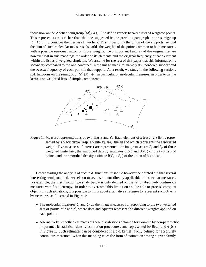
Figure 1: Measure representations of two listsz andz′. Each element ofz (resp. z′) list is repre-sented by a black circle (resp. a white square), the size of which represents the associatedweight. Five measures of interest are represented: the image measuresδz andδz′ of thoseweighted finite lists, the smoothed density estimatesθ(δz) andθ(δz′) of the two lists ofpoints, and the smoothed density estimateθ(δz+δz′) of the union of both lists.

Before starting the analysis of such p.d. functions, it should however bepointed out that severalinteresting semigroup p.d. kernels on measures are not directly applicable tomolecular measures.For example, the first function we study below is only defined on the set of absolutely continuousmeasures with finite entropy. In order to overcome this limitation and be able to process complexobjects in such situations, it is possible to think about alternative strategies to represent such objectsby measures, as illustrated in Figure 1:

• The molecular measuresδz andδz′ as the image measures corresponding to the two weightedsets of points ofz andz′, where dots and squares represent the different weights applied oneach points;

• Alternatively, smoothed estimates of these distributions obtained for example bynon-parametricor parametric statistical density estimation procedures, and represented byθ(δz) andθ(δz′)in Figure 1. Such estimates can be considered if a p.d. kernel is only defined for absolutelycontinuous measures. When this mapping takes the form of estimation among a given family

1173


of densities (through maximum likelihood for instance) this can also be seen asa prior beliefassumed on the distribution of the objects;

• Finally, a smoothed estimate of the sumδz+ δz′ corresponding to the merging of both lists,represented byθ(δz+δz′), can be considered. Note thatθ(δz+δz′) might differ fromθ(δz)+θ(δz′).

A kernel between two lists of points can therefore be derived from a p.d.function on(Mb+(X ),+)

in at least three ways:

k(z,z′) =

ϕ(δz+δz′), usingϕ directly on molecular measures,

ϕ(θ(δz)+θ(δz′)) , usingϕ on smoothed versions of the molecular measures,

ϕ(θ(δz+δz′)) , evaluatingϕ on a smoothed version of the sum.

The positive definiteness ofϕ on Mb+(X ) ensures positive definiteness ofk only in the first two

cases. The third expression can be seen as a special case of the firstone, where we highlight theusage of a preliminary mapping on the sum of two measures; in that caseϕ ◦ θ should in fact bep.d. on(Mb

+(X ),+), or at least(Mol+(X ),+). Having defined the set of representations on whichwe will focus in this paper, namely measures on a set of components, we propose in the followingsection two particular cases of positive definite functions that can be computed through an additionbetween the considered measures. We then show how those quantities can be computed in the caseof molecular measures in Section 4.

3. The Entropy and Inverse Generalized Variance Kernels

In this section we present two basic p.d. semigroup kernels for measures,motivated by a commonintuition: the kernel between two measures should increase when the sum ofthe measures getsmore “concentrated”. The two kernels differ in the way they quantify the concentration of a mea-sure, using either its entropy or its variance. They are therefore limited to a subset of measures,namely the subset of measures with finite entropy and the subset of sub-probability measures withnon-degenerated variance, but are extended to a broader class of measures, including molecularmeasures, in Section 4.

3.1 Entropy Kernel

We consider the subset ofMb+(X ) of absolutely continuous measures with respect to the dominant

measureν, and identify in this section a measure with its corresponding density with respect to ν.We further limit the subset to the set of non-negative valuedν-measurable functions onX with finitesum, such that

Mh+(X )

def= { f : X → R

+| f is ν-measurable, |h( f )| < ∞, | f | < ∞}

where we write for any measurable non-negative valued functiong,

h(g)def= −

Z

Xglngdν,

1174


(with 0 ln0= 0 by convention) and|g|def=

R

X gdν, consistently with the notation used for measures.If g is such that|g| = 1, h(g) is its differential entropy. Using the following inequalities,

(a+b) ln(a+b) ≤ alna+blnb+(a+b) ln2, by convexity ofx 7→ xlnx,

(a+b) ln(a+b) ≥ alna+blnb,

we have that(Mh+(X ),+) is an Abelian semigroup since forf , f ′ in Mh

+(X ) we have thath( f + f ′)is bounded by integrating pointwise the inequalities above, the boundedness of | f + f ′| being alsoensured. Following Rao (1987) we consider the quantity

J( f , f ′)def= h(

f + f ′

2)− h( f )+h( f ′)

2, (2)

known as theJensen divergence(or Jensen-Shannon divergence) betweenf and f ′, which as notedby Fuglede and Topsøe (2004) can be seen as a symmetrized version of the Kullback-Leibler (KL)divergenceD, since

J( f , f ′) =12

D( f || f + f ′

2)+

12

D( f ′|| f + f ′

2).

The expression of Equation (2) fits our framework of devising semigroupkernels, unlike the directuse of the KL divergence (Moreno et al., 2004) which is neither symmetric nor negative definite. Asrecently shown in Endres and Schindelin (2003) andOsterreicher and Vajda (2003),

√J is a metric

on Mh+(X ) which is a direct consequence ofJ’s negative definiteness proven below, through Berg

et al. (1984, Proposition 3.3.2) for instance. The Jensen-Divergence was also recently reinterpretedas a special case of a wider family of metrics onMb

+(X ) derived from a particular family of Hilber-tian metrics onR+ as presented in Hein and Bousquet (2005). The comparison between twoden-sities f , f ′ is in that case performed by integrating pointwise the squared distanced2( f (x), f ′(x))between the two densities overX , using ford a distance chosen among a suitable family of metricsin R+ to ensure that the final value is independent of the dominant measureν. The consideredfamily for d is described in Fuglede and Topsøe (2004) through two parameters, a family of whichthe Jensen Divergence is just a special case as detailed in Hein and Bousquet (2005). The latterwork shares with this paper another similarity, which lies in the “kernelization” of such quanti-ties defined on measures through a prior kernel on the space of components, as will be reviewedin Section 5. However, of all the Hilbertian metrics introduced in Hein and Bousquet (2005), theJensen-Divergence is the only one that can be related to the semigroup framework used throughoutthis paper.

Note finally that a positive definite kernelk is said to be infinitely divisible if− lnk is a negativedefinite kernel. As a consequence, any positive exponentiationkβ,β > 0 of an infinitely divisiblekernel is a positive definite kernel.

Proposition 1 h is a negative definite function on the semigroup Mh+(X ). As a consequence e−h

is a positive definite function on Mh+(X ) and its normalized counterpart, khdef= e−J is an infinitely

divisible positive definite kernel on Mh+(X )×Mh+(X ).

Proof It is known that the real-valued functionr : y 7→ −ylny is n.d. onR+ as a semigroup endowedwith addition (Berg et al., 1984, Example 6.5.16). As a consequence the function f 7→ r ◦ f is n.d.on Mh

+(X ) as a pointwise application ofr since r ◦ f is integrable w.r.tν. For any real-valuedn.d. kernelk and any real-valued functiong, we have trivially that(y,y′) 7→ k(y,y′)+ g(y)+ g(y′)

1175


remains negative definite. This allows first to prove thath( f+ f ′

2 ) is also n.d. through the identity

h( f+ f ′

2 ) = 12h( f + f ′)+ ln2

2 (| f |+ | f ′|). Subtracting the normalization factor12(h( f )+h( f ′)) gives

the negative definiteness ofJ. This finally yields the positive definiteness ofkh as the exponential ofthe negative of a n.d. function through Schoenberg’s theorem (Berg et al., 1984, Theorem 3.2.2).

Note that onlye−h is a semigroup kernel strictly speaking, sincee−J involves a normalized sum(through the division by 2) which is not associative. While bothe−h ande−J can be used in practiceon non-normalized measures, we name more explicitlykh = e−J theentropy kernel, because whatit indeed quantifies whenf and f ′ are normalized (i.e., such that| f | = | f ′| = 1) is the difference ofthe average of the entropy off and f ′ from the entropy of their average. The subset of absolutelycontinuousprobability measures on(X ,ν) with finite entropies, namely

{

f ∈ Mh+(X ), s.t.| f | = 1

}

is not a semigroup since it is not closed by addition, but we can nonethelessdefine the restriction ofJand hencekh on it to obtain a p.d. kernel on probability measures inspired by semigroup formalism.

3.2 Inverse Generalized Variance Kernel

We assume in this subsection thatX is an Euclidian space of dimensionn endowed with Lebesgue’smeasureν. Following the results obtained in the previous section, we propose under these re-strictions a second semigroup p.d. kernel between measures which uses generalized variance. Thegeneralized variance of a measure, namely the determinant of its variance matrix, is a quantity ho-mogeneous to a volume inX . This volume can be interpreted as a typical volume occupied by ameasure when considering only its second order moments, making it hence a useful quantificationof its dispersion. Besides being easy to compute in the case of molecular measures, this quantity isalso linked to entropy if we consider that for normal lawsN (m,Σ) the following relation holds:

1√detΣ

∝ e−h(N (m,Σ)).

Through this observation, we note that considering the Inverse of the Generalized Variance (IGV)of a measure is equivalent to considering the value taken bye−2h on its maximum likelihood normallaw. We will put aside this interpretation in this section, before reviewing it with more care inSection 7.

Let us define the variance operator on measuresµ with finite first and second moment ofMb+(X )

asΣ(µ)

def= µ[xx>]−µ[x]µ[x]>.

Note thatΣ(µ) is always a positive semi-definite matrix whenµ is a sub-probability measure, that iswhen|µ| ≤ 1, since

Σ(µ) = µ[(x−µ[x])(x−µ[x])>]+ (1−|µ|)µ[x]µ[x]>.

We call detΣ(µ) the generalized variance of a measureµ, and say a measureµ is non-degeneratedifdetΣ(µ) is non-zero, meaning thatΣ(µ) is of full rank. The subset ofMb

+(X ) of such measures withtotal weight equal to 1 is denoted byMv

+(X ); Mv+(X ) is convex through the following proposition:

Proposition 2 Mv+(X )

def={

µ∈ Mb+(X ) : |µ| = 1,detΣ(µ) > 0

}

is a convex set, and more generallyfor λ ∈ [0,1), µ′ ∈ Mb

+(X ) such that|µ′| = 1 and µ∈ Mv+(X ), (1−λ)µ+λµ′ ∈ Mv

+(X ).

1176


Proof We use the following identity,

Σ(

(1−λ)µ+λµ′)

= (1−λ)Σ(µ)+λΣ(µ′)+λ(1−λ)(

µ[x]−µ′[x])(

µ[x]−µ′[x])>

,

to derive thatΣ((1− λ)µ+ λµ′) is a (strictly) positive-definite matrix as the sum of two positivesemi-definite matrices and a strictly positive definite matrixΣ(µ).

Mv+(X ) is not a semigroup, since it is not closed under addition. However we will work in this

case on the mean of two measures in the same way we used their standard addition in the semigroupframework ofMb

+(X ).

Proposition 3 The real-valued kernel kv defined on elements µ,µ′ of Mv+(X ) as

kv(µ,µ′) =1

detΣ(µ+µ′2 )

is positive definite.

Proof Let y be an element ofX . For anyN ∈ N, anyc1, ...,cN ∈ R such that∑i ci = 0 and anyµ1, ...,µN ∈ Mv

+(X ) we have

∑i, j

cic jy>Σ(

µi +µj

2)y = ∑

i, j

cic jy>(

12

µi [xx>]+12

µj [xx>]−

14

(

µi [x]µi [x]> +µj [x]µj [x]

> +µj [x]µi [x]> +µi [x]µj [x]

>)

)

y

= −14 ∑

i, j

cic jy>(

µj [x]µi [x]> +µi [x]µj [x]

>)

y

= −12

(

∑i

ciy>µi [x]

)2

≤ 0,

making thus the functionµ,µ′ 7→ y>Σ(µ+µ′

2 )y negative-definite for anyy∈ X . Using again Schoen-

berg’s theorem (Berg et al., 1984, Theorem 3.2.2) we have thatµ,µ′ 7→ e−y>Σ( µ+µ′2 )y is positive defi-

nite and so is the sum 1(2π)

n2

R

X e−y>Σ( µ+µ′2 )yν(dy) which is equal to 1/

√

detΣ(µ+µ2 ) ensuring thus the

positive-definiteness ofkv as its square.

Both entropy and IGV kernels are defined on subsets ofMb+(X ). Since we are most likely to use

them on molecular measures or smooth measures (as discussed in Section 2.2),we present in thefollowing section practical ways to apply them in that framework.

4. Semigroup Kernels on Molecular Measures

The two positive definite functions defined in Sections 3.1 and 3.2 cannot beapplied in the generalcase to Mol+(X ) which as exposed in Section 2 is our initial goal. In the case of the entropykernel, molecular measures are generally not absolutely continuous with respect toν (except on

1177


finite spaces), and they have therefore no entropy; we solve this problem by mapping them intoMh

+(X ) through a smoothing kernel. In the case of the IGV, the estimates of variances might bepoor if the number of points in the lists is not large enough compared to the dimension of theEuclidean space; we perform in that case a regularization by adding a unit-variance correlationmatrix to the original variance. This regularization is particularly important to pave the way to thekernelized version of the IGV kernel presented in the next section, when X is not Euclidian butsimply endowed with a prior kernelκ.

The application of both the entropy kernel and the IGV kernel to molecular measures requires aprevious renormalization to set the total mass of the measures to 1. This technical renormalizationis also beneficial, since it allows a consistent comparison of two weighted lists even when theirsize and total mass is very different. All molecular measures in this section, and equivalently alladmissible bases, will hence be supposed to be normalized such that their total weight is 1, andMol1+(X ) denotes the subset of Mol+(X ) of such measures.

4.1 Entropy Kernel on Smoothed Estimates

We first define the Parzen smoothing procedure which allows to map molecularmeasures ontomeasures with finite entropy:

Definition 4 Let κ be a probability kernel onX with finite entropy, i.e., a real-valued functiondefined onX 2 such that for any x∈X , κ(x, ·) : y 7→ κ(x,y) satisfiesκ(x, ·)∈Mh

+(X ) and|κ(x, ·)|= 1.Theκ-Parzen smoothed measure of µ is the probability measure whose densitywith respect toν isθκ(µ), where

θκ :Mol1+(X ) −→ Mh+(X )

µ 7→ ∑x∈suppµ

µ(x)κ(x, ·).

Note that for any admissible base(xi ,ai)dk=1 of µ we have thatθκ(µ) = ∑d

i=1aiκ(xi , ·). Once thismapping is defined, we use the entropy kernel to propose the following kernel on two molecularmeasuresµ andµ′,

kκh(µ,µ′) = e−J(θκ(µ),θκ(µ′)).

As an example, letX be an Euclidian space of dimensionn endowed with Lebesgue’s measure,andκ the isotropic Gaussian RBF kernel on that space, namely

κ(x,y) =1

(2πσ)n2e−

‖x−y‖2

2σ2 .

Given two weighted listsz and z′ of components inX , θκ(δz) and θκ(δz′) are thus mixtures ofGaussian distributions onX . The resulting kernel computes the entropy ofθκ(δz) andθκ(δz′) takenseparately and compares it with that of their mean, providing a positive definite quantification oftheir overlap.

4.2 Regularized Inverse Generalized Variance of Molecular Measures

In the case of a molecular measureµ defined on an Euclidian spaceX of dimensionn, the varianceΣ(µ) is simply the usual empirical estimate of the variance matrix expressed in an orthonormal basis

1178


of X :

Σ(µ) = µ[xx>]−µ[x]µ[x]> =d

∑i=1

aixix>i −

(

d

∑i=1

aixi

)(

d

∑i=1

aixi

)>

,

where we use an admissible baseγ = (xi ,ai)di=1 of µ to give a matrix expression ofΣ(µ), with all

pointsxi expressed as column vectors. Note that this matrix expression, as would beexpected froma function defined on measures, does not depend on the chosen admissible base. Given such anadmissible base, letXγ = [xi ]i=1..d be then× d matrix made of all column vectorsxi and∆γ thediagonal matrix of weights ofγ taken in the same order(ai)1≤ı≤d. If we write Id for the identitymatrix of rankd and

�d,d for thed×d matrix composed of ones, we have for any baseγ of µ that:

Σ(µ) = Xγ(∆γ −∆γ�

d,d∆γ)X>γ ,

which can be rewritten as

Σ(µ) = Xγ(Id −∆γ�

d,d)∆γ(Id −�

d,d∆γ)X>γ ,

noting that(∆γ�

d,d)2 = ∆γ

�d,d since trace∆γ = 1.

The determinant ofΣ(µ) can be equal to zero when the size of the support ofµ is smaller thann, the dimension ofX , or more generally when the linear span of the points in the support ofµdoes not cover the whole spaceX . This problematic case is encountered in Section 5 when weconsider kernelized versions of the IGV, using an embedding ofX into a functional Hilbert spaceof potentially infinite dimension. Mapping an element of Mol1

+(X ) into Mv+(X ) by adding to it any

element ofMv+(X ) through Proposition 2 would work as a regularization technique; for an arbitrary

ρ ∈ Mv+(X ) and a weightλ ∈ [0,1) we could use the kernel defined as

µ,µ′ 7→ 1

detΣ(

λµ+µ′2 +(1−λ)ρ

) .

We use in this section a different strategy inspired by previous works (Fukumizu et al., 2004,Bach and Jordan, 2002) further motivated in the case of covariance operators on infinite dimensionalspaces as shown by Cuturi and Vert (2005). The considered regularization consists in modifyingdirectly the matrixΣ(µ) by adding a small diagonal componentηIn whereη > 0 so that its spectrumnever vanishes. When considering the determinant of such a regularized matrix Σ(µ)+ ηIn this isequivalent to considering the determinant of1

η Σ(µ) + In up to a factorηn, which will be a more

suitable expression in practice. We thus introduce the regularized kernelkηv defined on measures

(µ,µ′) ∈ Mb+(X ) with finite second moment as

kηv (µ,µ′)

def=

1

det(

1η Σ(

µ+µ′2

)

+ In) .

It is straightforward to prove that the regularized functionkηv is a positive definite kernel on the

measures ofMb+(X ) with finite second-order moments using the same proof used in Proposition 3.

If we now introduceKγ

def=[

x>i x j

]

1≤i, j≤d,

1179


for thed×d matrix of dot-products associated with the elements of a baseγ, and

Kγdef=

[

(xi −d

∑k=1

akxk)>(x j −

d

∑k=1

akxk)

]

1≤i, j≤d

= (Id −�

d,d∆γ)Kγ(Id −∆γ�

d,d),

for its centered expression with respect to the mean ofµ, we have the following result:

Proposition 5 Let X be an Euclidian space of dimension n. For any µ∈ Mol1+(X ) andanyadmis-sible baseγ of µ we have

det

(

1η

Kγ∆γ + Il(γ)

)

= det

(

1η

Σ(µ)+ In

)

.

Proof We omit the references toµ and γ in this proof to simplify matrix notations, and writed = l(γ). Let X be then×d matrix [xi −∑d

j=1a jx j ]i=1..d of centered column vectors enumerated inγ, namelyX = X(Id −∆

�d,d). We have

Σ = X∆X>,

K∆ = X>X∆.

Through the singular value decomposition ofX∆ 12 , it is straightforward to see that the non-zero

elements of the spectrums of matricesK∆,∆ 12 X>X∆ 1

2 andΣ are identical. Thus, regardless of thedifference betweenn andd, we have

det

(

1η

K∆+ Id

)

= det

(

1η

∆12 X>X∆

12 + Id

)

= det

(

1η

X∆X> + In

)

= det

(

1η

Σ+ In

)

,

where the addition of identity matrices only introduces an offset of 1 for all eigenvalues.

Given two measuresµ,µ′ ∈Mol1+(X ), the following theorem can be seen as a regularized equivalent

of Proposition 3 through an application of Proposition 5 toµ′′ = µ+µ′

2 .

Theorem 6 Let X be an Euclidian space. The kernel kηv defined on two measures µ,µ′ of Mol1+(X )

as

kηv (µ,µ′) =

1

det(

1η Kγ∆γ + Il(γ)

) ,

whereγ is any admissible base ofµ+µ′

2 , is p.d. and independent of the choice ofγ.

Given two objectsz,z′ and their respective molecular measuresδz andδz′ , the computation of the

IGV for two such objects requires in practice an admissible base ofδz+δz′2 as seen in Theorem 6. This

admissible base can be chosen to be of the cardinality of the support of the mixture ofδz andδz′ , oralternatively be the simple merger of two admissible bases ofzandz′ with their weights divided by2, without searching for overlapped points between both lists. This choicehas no impact on the finalvalue taken by the regularized IGV-kernel and can be arbitrated by computational considerations.

If we now take a practical look at the IGV’s definition, we note that it can beapplied but to caseswhere the component spaceX is Euclidian, and only if the studied measures can be summarizedefficiently by their second order moments. These limitations do not seem very realistic in practice,

1180


sinceX may not have a vectorial structure, and the distribution of the components maynot evenbe well represented by Gaussians in the Euclidian case. We propose to bypass this issue and intro-duce the usage of the IGV in a more flexible framework by using the kernel trick on the previousquantities, since the IGV of a measure can be expressed only through the dot-products between theelements of the support of the considered measure.

5. Inverse Generalized Variance on the RKHS Associated witha Kernel κ

As with many quantities defined by dot-products, one is tempted to replace the usual dot-productmatrix K of Theorem 6 by an alternative Gram-matrix obtained through a p.d. kernelκ definedon X . The advantage of such a substitution, which follows the well known “kernel trick” princi-ple (Scholkopf and Smola, 2002), is multiple as it first enables us to use the IGV kernel on anynon-vectorial space endowed with a kernel, thus in practice on any component space endowed witha kernel; second, it is also useful whenX is a dot-product space where a non-linear kernel canhowever be used (e.g., using Gaussian kernel) to incorporate into the IGV’s computation higher-order moment comparisons. We prove in this section that the inverse of the regularized generalizedvariance, computed in Proposition 5 through the centered dot-product matrix Kγ of elements of anyadmissible baseγ of µ, is still a positive definite quantity if we replaceKγ by a centered Gram-matrixKγ, computed through an a priori kernelκ on X , namely

Kγ = [κ(xi ,x j)]1≤i, j≤d

Kγ = (Id −�

d,d∆γ)Kγ(Id −∆γ�

d,d).

This substitution follows also a general principle when considering kernelson measures. The “ker-nelization” of a given kernel defined on measures to take into account a prior similarity on thecomponents, when computationally feasible, is likely to improve its overall performance in classifi-cation tasks, as observed in Kondor and Jebara (2003) but also in Heinand Bousquet (2005) underthe “Structural Kernel” appellation. The following theorem proves that thissubstitution is valid inthe case of the IGV.

Theorem 7 Let X be a set endowed with a p.d. kernelκ. The kernel

kηκ(µ,µ′) =

1

det(

1η Kγ∆γ + Il(γ)

) , (3)

defined on two elements µ,µ′ in Mol1+(X ) is positive definite, whereγ is anyadmissible base ofµ+µ′

2 .

Proof LetN∈N, µ1, ..,µN ∈Mol1+(X ) and(ci)Ni=1∈R

N. Let us now study the quantity∑Ni=1cic j k

ηκ(µi ,µj).

To do so we introduce by the Moore-Aronszajn theorem (Berlinet and Thomas-Agnan, 2003, p.19)the reproducing kernel Hilbert spaceΞ with reproducing kernelκ indexed onX . The usual mappingfrom X to Ξ is denoted byφ, that isφ : X 3 x 7→ κ(x, ·). We define

Ydef= supp

(

N

∑i=1

µi

)

⊂ X ,

the finite set which numbers all elements in the support of theN considered measures, and

ϒdef= spanφ(Y ) ⊂ Ξ,

1181


the linear span of the elements in the image ofY throughφ. ϒ is a vector space whose finitedimension is upper-bounded by the cardinality ofY . Endowed with the dot-product inherited fromΞ, we further have thatϒ is Euclidian. Given a molecular measureµ∈Mol1+(Y ), letφ(µ) denote theimage measure ofµ in ϒ, namelyφ(µ) = ∑x∈Y µ(x)δφ(x). One can easily check that any admissible

baseγ = (xi ,ai)di=1 of µ can be used to provide an admissible baseφ(γ)def

= (φ(xi),ai)di=1 of φ(µ).

The weight matrices∆γ and∆φ(γ) are identical and we further haveKγ = Kφ(γ) by the reproducingproperty, whereK is defined by the dot-product of the Euclidian spaceϒ induced byκ. As aresult, we have thatkη

κ(µi ,µj) = kηv (φ(µi),φ(µj)) wherekη

v is defined on Mol1+(ϒ), ensuring thenon-negativity

N

∑i=1

cic j kηκ(µi ,µj) =

N

∑i=1

cic j kηv (φ(µi),φ(µj)) ≥ 0

and hence positive-definiteness ofkηκ .

As bserved in the experimental section, the kernelized version of the IGV ismore likely to be suc-cessful to solve practical tasks since it incorporates meaningful information on the components. Be-fore observing these practical improvements, we provide a general study of the family of semigroupkernels onMb

+(X ) by casting the theory of integral representations of positive definite functions ona semigroup (Berg et al., 1984) in the framework of measures, providing new results and possibleinterpretations of this class of kernels.

6. Integral Representation of Positive Definite Functions on a Set of Measures

In this section we study a general characterization ofall p.d. functions on the whole semigroup(Mb

+(X ),+), including thus measures which are not normalized. This characterization is based ona general integral representation theorem valid for any semigroup kernel, and is similar in spirit tothe representation of p.d. functions obtained on Abelian groups through Bochner’s theorem (Rudin,1962). Before stating the main results in this section we need to recall basic definitions of semichar-acters and exponentially bounded function (Berg et al., 1984, chap. 4).

Definition 8 A real-valued functionρ on an Abelian semigroup(S,+) is called asemicharacterifit satisfies the following properties:

(i) ρ(0) = 1

(ii) ∀s, t ∈ S,ρ(s+ t) = ρ(s)ρ(t).

It follows from the previous definition and the fact thatMb+(X ) is2-divisible(i.e.,∀µ∈Mb

+(X ),∃µ′ ∈Mb

+(X ) s.t. µ = 2µ′) that semicharacters are nonnegative valued since it suffices to write thatρ(µ) = ρ(µ

2)2. Note also that semicharacters are trivially positive definite functions onS. We de-note byS∗ the set of semicharacters onMb

+(X ), and byS⊂ S∗ the set of bounded semicharacters.S∗ is a Hausdorff space when endowed with the topology inherited fromR

S having the topologyof pointwise convergence. Therefore we can consider the set of Radon measures onS∗, namelyMb

+(S∗).

Definition 9 A function f : Mb+(X ) → R is calledexponentially boundedif there exists a function

α : Mb+(X ) → R+ (called anabsolute value) satisfyingα(0) = 1 and α(µ+ µ′) ≤ α(µ)α(µ′) for

1182


µ,µ′ ∈ Mb+(X ), and a constant C> 0 such that:

∀µ∈ Mb+(X ), f (µ) ≤Cα(µ).

We can now state two general integral representation theorems for p.d. functions on semigroups (Berget al., 1984, Theorems 4.2.5 and 4.2.8). These theorems being valid on any semigroup, they hold inparticular on the particular semigroup(Mb

+(X ),+).

Theorem 10 • A functionϕ : Mb+(X ) → R is p.d. and exponentially bounded if and only if it

has an integral representation:

ϕ(s) =Z

S∗ρ(s)dω(ρ),

with ω ∈ Mc+(S∗) (the set of Radon measures on S∗ with compact support).

• A functionϕ : Mb+(X )→ R is p.d. and bounded if and only if it has an integral representation

of the form:

ϕ(s) =Z

Sρ(s)dω(ρ),

with ω ∈ M+(S).In both cases, if the integral representation exists, then there is uniqueness of the measureω in

M+(S∗).

In order to make these representations more constructive, we need to study the class of (bounded)semicharacters on(Mb

+(X ),+). Even though we are not able to provide a complete characterization,even of bounded semicharacters, the following proposition introduces a large class of semicharac-ters, and completely characterizes thecontinuoussemicharacters. For matters related to continuityof functions defined onMb

+(X ), we will consider the weak topology ofMb+(X ) which is defined in

simple terms through theportmanteautheorem (Berg et al., 1984, Theorem 2.3.1). Note simply thatif µn converges toµ in the weak topology then for anyboundedmeasurable and continuous functionf we have thatµn[ f ]→ µ[ f ]. We further denote byC(X ) the set of continuous real-valued functionson X and byCb(X ) its subset of bounded functions. Both sets are endowed with the topology ofpointwise convergence. For a functionf ∈ R

X we write ρ f for the functionµ 7→ eµ[ f ] when theintegral is well defined.

Proposition 11 A semicharacterρ : Mb+(X ) → R is continuous on(Mb

+(X ),+) endowed with theweak topology if and only if there exists f∈Cb(X ) such thatρ = ρ f . In that case,ρ is a boundedsemicharacter on Mb+(X ) if and only if f ≤ 0.

Proof For a continuous and bounded functionf , the semicharacterρ f is well-defined. If a sequenceµn in Mb

+(X ) converges toµ weakly, we haveµn[ f ] → µ[ f ], which implies the continuity ofρ f .Conversely, supposeρ is weakly continuous. Definef : X → [−∞,∞) by f (x) = logρ(δx). If asequencexn converges tox in X , obviously we haveδxn → δx in the weak topology, and

ρ(δxn) → ρ(δx),

1183


which means the continuity off . To see the boundedness off , assume the contrary. Then, we canfind xn ∈ X such that either of 0< f (xn)→ ∞ or 0> f (xn)→−∞ holds. Letβn = | f (xn)|. Becausethe measure1

βnδxn converges weakly to zero, the continuity ofρ means

ρ(

1βn

δxn

)

→ 1,

which contradicts with the factρ( 1βn

δxn) = e1

βnf (xn) = e±1. Thus,ρ f is well-defined, weakly contin-

uous onMb+(X ) and equal toρ on the set of molecular measures. It is further equal toρ on Mb

+(X )through the denseness of molecular measures inMb

+(X ), both in the weak and the pointwise topol-ogy (Berg et al., 1984, Proposition 3.3.5). Finally suppose now thatρ f is bounded and that thereexistsx in X such thatf (x) > 0. By ρ f (nδx) = en f(x) which diverges withn we see a contradiction.The converse is straightforward.

Let ω be a bounded nonnegative Radon measure on the Hausdorff space ofcontinuous real-valuedfunctions onX , namelyω ∈ Mb

+(C(X )). Given such a measure, we first define the subsetMω ofMb

+(X ) asMω = {µ∈ Mb

+(X ) | supf∈suppω

µ[ f ] < +∞}.

Mω contains the null measure and is a semigroup.

Corollary 12 For any bounded Radon measureω ∈ Mb+(C(X )), the following functionϕ is a

p.d. function on the semigroup(Mω,+):

ϕ(µ) =Z

C(X )ρ f (µ) dω( f ). (4)

If suppω ⊂Cb(X ) thenϕ is continuous on Mω endowed with the topology of weak convergence.

Proof For f ∈ suppω, ρ f is a well defined semicharacter onMω and hence positive definite. Since

ϕ(µ) ≤ |ω| supf∈suppω

µ[ f ]

is bounded,ϕ is well defined and hence positive definite. Suppose now that suppω ⊂ Cb(X ) andlet µn be a sequence ofMω converging weakly toµ. By the bounded convergence theorem andcontinuity of all considered semicharacters (since all considered functions f are bounded) we havethat:

limn→∞

ϕ(µn) =Z

C(X )limn→∞

ρ f (µn) dω( f ) = ϕ(µ).

and henceϕ is continuous w.r.t the weak topology.

When the measureω is chosen in such a way that the integral (4) is tractable or can be approximated,then a valid p.d. kernel for measures is obtained; an example involving mixtures over exponentialfamilies is provided in Section 7.

Before exploiting this constructive representation, a few remarks shouldbe pointed out. Whenusing non-bounded functions (as is the case when using expectation or second-order moments ofmeasures) the continuity of the integralϕ is left undetermined to our knowledge, even when itsexistence is ensured. However, whenX is compact we have thatC(X )=Cb(X ) and hence continuity

1184


on Mω of any functionϕ constructed through corollary 12. Conversely, there exist continuousp.d. functions on(Mb

+(X ),+) that can not be represented in the form (4). Although any continuousp.d. function can necessarily be represented as an integral of semicharacters by Theorem 10, thesemicharacters involved in the representation are not necessarily continuous as in (4). An example ofsuch a continuous p.d. function written as an integral of non-continuous semicharacters is exposed inAppendix A. It is an open problem to our knowledge to fully characterize continuous p.d. functionson (Mb

+(X ),+).

7. Projection on Exponential Families through Laplace’s Approximation

The constructive approach presented in corollary 12 can be used in practice to define kernels byrestricting the spaceC(X ) to subspaces where computations are tractable. A natural way to do so isto consider a vector space of finite dimensions of C(X ), namely the span of a free family ofs non-constant functionsf1, ..., fs of C(X ), and define a measure on that subspace by applying a measureon the weights associated with each function. The previous integral representation (4) would thentake the form:

ϕ(µ) =Z

Θeµ[∑s

i=1 θi fi ] ω(dθ),

whereω is now a bounded measure on a compact subsetΘ ⊆ Rs andµ is such thatµ[ fi ] < +∞ for

1≤ i ≤ s. The subspace ofC(X ) considered in this section is however slightly different, in order totake advantage of the natural benefits of exponential densities generated by all functionsf1, ..., fs.Following Amari and Nagaoka (2001, p.69), this requires the definition of the cumulant generatingfunction ofν with respect tof1, ..., fs as

ψ(θ)def= logν[e∑s

i=1 θi fi ],

such that for eachθ ∈ Θ,

pθdef= exp

(

s

∑i=1

θi fi −ψ(θ)

)

ν,

is a probability density, which defines an exponential family of densities onX asθ varies inΘ.Rather than the direct span of functionsf1, ..., fs on Θ, this is equivalent to considering the hyper-surface{∑s

i=1 θi fi −ψ(θ)} in span{ f1, .., fs,−1}. This yields the following expression:

ϕ(µ) =Z

Θeµ[∑s

i=1 θi fi−ψ(θ)] ω(dθ).

Following the notations of Amari and Nagaoka (2001) theη-parameters (or expectation parameters)of µ are defined as

ηidef=

1|µ|µ[ fi ], 1≤ i ≤ s,

andθ stands for theθ-parameters ofη. We assume in the following approximations thatθ ∈ Θ andrecall two identities (Amari and Nagaoka, 2001, Chapters 3.5 & 3.6):

χ(θ)def=

s

∑i=1

θiηi −ψ(θ) = −h(θ), the dual potential,

D(θ||θ′) = ψ(θ)+χ(θ′)−s

∑i=1

θiη′i , the KL divergence,

1185


where we used the abbreviationsh(θ) = h(pθ) andD(θ||θ′) = D(pθ||pθ′). We can then write

µ[s

∑i=1

θi fi −ψ(θ)] = |µ|(

s

∑i=1

θiηi −ψ(θ)

)

= |µ|(

s

∑i=1

θiηi −ψ(θ)+s

∑i=1

(θi − θi)ηi +ψ(θ)−ψ(θ)

)

= −|µ|(

h(θ)+D(θ||θ))

,

to obtain the following factorized expression,

ϕ(µ) = e−|µ|h(θ)Z

Θe−|µ|D(θ||θ)ω(dθ). (5)

The quantitye−|µ|h(θ) was already evoked in Section 3.2 when multivariate normal distributionswere used to express the IGV kernel. WhenX is an Euclidian space of dimensionn, this is indeedequivalent to definings = n+ n(n+ 1)/2 base functions, more preciselyfi = xi and fi j = xix j ,and dropping the integral of Equation (5). Note that such functions are not bounded and thatMωcorresponds here to the set of measures with finite first and second order moments.

The integral of Equation (5) cannot be computed in a general case. Theuse of conjugate priorscan however yield exact calculations, such as in the setting proposed by Cuturi and Vert (2005).In their workX is a finite set of short sequences formed over an alphabet, functionsfi are all pos-sible indicator functions ofX andω is an additive mixture of Dirichlet priors. The kernel valueis computed through a factorization inspired by the context-tree weighting algorithm (Willemset al., 1995). In the general case a numerical approximation can also be derived using Laplace’smethod (Dieudonne, 1968) under the assumption that|µ| is large enough. To do so, first notice that

∂D(θ||θ)

∂θi|θ= θ =

∂ψ∂θi

|θ= θ −ηi = 0,

∂D(θ||θ)

∂θi∂θ j=

∂ψ∂θi∂θ j

= gi j (θ),

whereGθ = [gi j (θ)] is the Fisher information matrix computed inθ and hence a p.d. matrix. Thefollowing approximation then holds:

ϕ(µ) ∼|µ|→∞

e−|µ|h(θ)Z

Rsω(θ)e−

|µ|2 (θ−θ)>Gθ(θ−θ)dθ = e−|µ|h(θ)

(

2π|µ|

)s2 ω(θ)√

detGθ

which can be simplified by choosingω to be Jeffrey’s prior (Amari and Nagaoka, 2001, p.44),namely

ω(dθ) =1V

√

detGθ dθ, whereV =Z

Θ

√

detGθ dθ.

Up to a multiplication byV this provides an approximation ofϕ by ϕ as

ϕ(µ) ∼|µ|→∞

ϕ(µ)def= e−|µ|h(θ)

(

2π|µ|

)s2

.

1186


The η-coordinates ofµ are independent of the total weight|µ|, henceϕ(2µ) = ϕ(µ)2( |µ|4π )

s2 . This

identity can be used to propose a renormalized kernel for two measures as

k(µ,µ′)def=

ϕ(µ+µ′)√

ϕ(2µ)ϕ(2µ′)=

e−(|µ+µ′|)h(pµ+µ′ )

e−|µ|h(pµ)−|µ′|h(pµ′ )

(

2√

|µ||µ′||µ|+ |µ′|

)s2

.

wherepµ stands forpθµ. Whenµ andµ′ are normalized such that their total weight coincides and is

equal toβ, we have that

k(µ,µ′) = e−2β

(

h(pµ′′ )−h(pµ)+h(pµ′ )

2

)

, (6)

whereµ′′ = µ+ µ′. From Equation (6), we see thatβ can be tuned in practice and thought of as awidth parameter. It should be large enough to ensure the consistency of Laplace’s approximationand thus positive definiteness, while not too large at the same time to avoid diagonal dominanceissues. In the case of the IGV kernel this tradeoff can however be putaside since the inverse of theIGV is directly p.d. as was proved in Proposition 3. However and to our knowledge this assertiondoes not stand in a more general case when the functionsf1, ..., fs are freely chosen.

8. Experiments on Images of the MNIST Database

We present in this section experimental results and discussions on practical implementations ofthe IGV kernels on a benchmark experiment of handwritten digits classification. We focus morespecifically on the kernelized version of the IGV and discuss its performance with respect to otherkernels. The entropy kernel performed very poorly in the series of experiments presented here,besides requiring a time consuming Monte Carlo computation, which is why we do not considerit in this section. We believe however that in more favourable cases, notablywhen the consideredmeasures are multinomials, the entropy kernel and its structural variants (Hein and Bousquet, 2005)may provide good results.

8.1 Linear IGV Kernel

Following the previous work of Kondor and Jebara (2003), we have conducted experiments on 500and 1000 images (28× 28 pixels) taken from the MNIST database of handwritten digits (blackshapes on a white background), with 50 (resp. 100) images for each digit. To each imagez werandomly associate a set ofd distinct points which are black (intensity superior to 190) in theimage. In this case the set of components is{1, ..,28}× {1, ..,28} which we map onto pointswith coordinates between 0 and 1, thus definingX = [0,1]2. The linear IGV kernel as describedin Section 3.2 is equivalent to using the linear kernelκ((x1,y1),(x2,y2)) = x1x2 + y1y2 on a non-regularized version of the kernelized-IGV. It also boils down to fitting Gaussian bivariate-laws onthe points and measuring the similarity of two measures by performing variance estimation on thesamples taken first separately and then together. The resulting variancescan be diagonalized toobtain three diagonal variance matrices, which can be seen as performingPCA on the sample,

Σ(µ) =

(

Σ1,1 00 Σ2,2

)

, Σ(µ′) =

(

Σ′1,1 00 Σ′

2,2

)

, Σ(µ′′) =

(

Σ′′1,1 00 Σ′′

2,2

)

.

1187


and the value of the kernel is computed through

kv(µ,µ′) =

√

Σ1,1Σ2,2 Σ′1,1Σ′

2,2

Σ′′1,1Σ′′

2,2.

This ratio is for instance equal to 0.3820 for two handwritten digits in the case shown in Figure 2.The linear IGV manages a good discrimination between ones and zeros. Indeed, ones are shaped

0 5 10 15 20 250

5

10

15

20

25

x

y

0 5 10 15 20 250

5

10

15

20

25

x

y

0 5 10 15 20 250

5

10

15

20

25

x

y

Σ1,1 = 0.0552 Σ′1,1 = 0.0441 Σ′′

1,1 = 0.0497Σ2,2 = 0.0013 Σ′

2,2 = 0.0237 Σ′′2,2 = 0.0139

Figure 2: Weighted PCA of two different measures and their mean, with their first principal com-ponent shown. Below are the variances captured by the first and second principal compo-nents, the generalized variance being the product of those two values.

as sticks, and hence usually have a strong variance carried by their first component, followed bya weak second component. On the other hand, the variance of zeros is more equally distributedbetween the first and second axes. When both weighted sets of points areunited, the varianceof the mean of both measures has an intermediary behaviour in that respect,and this suffices todiscriminate numerically both images. However this strategy fails when using numbers which arenot so clearly distinct in shape, or more precisely whose surface cannot be efficiently expressed interms of Gaussian ellipsoids. To illustrate this we show in Figure 3 the Gram matrix of the linearIGV on 60 images, namely 20 zeros, 20 ones and 20 twos. Though images ofones can be efficientlydiscriminated from the two other digits, we clearly see that this is not the case between zeros andtwos, whose support may seem similar if we try to capture them through Gaussian laws. In practice,the results obtained with the linear IGV on this particular task where so unadapted to the learninggoal that the SVM’s trained based on that methodology did not converge inmost cases, which iswhy we discarded it.

8.2 Kernelized IGV

Following previous works (Kondor and Jebara, 2003, Wolf and Shashua, 2003) and as suggested inthe initial discussion of Section 5, we use in this section a Gaussian kernel ofwidth σ to incorporatea prior knowledge on the pixels, and equivalently to define the reproducing kernel Hilbert spaceΞby using

κ((x1,y1),(x2,y2)) = e−(x1−x2)2+(y1−y2)2

2σ2 .

1188


0 1 2

0

1

2

Figure 3: Normalized Gram matrix computed with the linear IGV kernel of twenty images of “0”,“1” and “2” displayed in that order. Darker spots mean values closer to 1, showing thatthe restriction to “0” and “1” yields good separation results, while “0” and “2” can hardlybe discriminated using variance analysis.

As pointed out by Kondor and Jebara (2003), the pixels are no longer seen as points but rather asfunctions (Gaussian bells) defined on the components space[0,1]2. To illustrate this approach weshow in Figure 4 the first four eigenfunctions of three measuresµ1, µ0 and µ1+µ0

2 built from theimage of a handwritten “1” and “0” with their corresponding eigenvalues, as well as for images of“2” and “0” in Figure 5.

Settingσ, the width ofκ, to define the functions contained in the RKHSΞ is not enough to fullycharacterize the values taken by the kernelized IGV. We further need to defineη, the regularizationparameter, to control the weight assigned to smaller eigenvalues in the spectrum of Gram matrices.Both parameters are strongly related, since the value ofσ controls the range of the typical eigen-values found in the spectrum of Gram matrices of admissible bases, whereas η acts as a scalingparameter for those eigenvalues as can be seen in Equation (3). Indeed, using a very smallσ value,which meansΞ is only defined by peaked Gaussian bells around each pixels, yields diagonally dom-inant Gram matrices very close to the identity matrix. The resulting eigenvalues for K ∆ are thenall very close to1

d , the inverse of the amount of considered points. On the contrary, a largevaluefor σ yields higher values for the kernel, since all points would be similar to each other and Grammatrices would turn close to the matrix

�d,d with a single significant eigenvalue and all others close

to zero. We address these issues and study the robustness of the final output of the k-IGV kernel interms of classification error by doing preliminary experiments where bothη andσ vary freely.

8.3 Experiments on the SVM Generalization Error

To study the behaviour and the robustness of the IGV kernel under different parameter settings, weused two ranges of values forη andσ:

1189


0.276 0.168 0.184

0.169 0.142 0.122

0.124 0.119 0.0934

0.0691 0.0962 0.0886

Figure 4: The four first eigenfunctions of respectively three empiricalmeasuresµ1 (first column),µ0 (second column) andµ1+µ0

2 (third column), displayed with their corresponding eigen-values, usingη = 0.01 andσ = 0.1.

1190


0.146 0.168 0.142

0.141 0.142 0.122

0.127 0.119 0.103

0.119 0.0962 0.0949

Figure 5: Same representation as in Figure 4, withµ2, µ0 and µ2+µ02 .

1191


η ∈ 10−2×{0.1,0.3,0.5,0.8,1,1.5,2,3,5,8,10,20}σ ∈ {0.05,0.1,0.12,0.15,0.18,0.20,0.25,0.3}.

For each kernelkηκ defined by a (σ,η) couple, we trained 10 binary SVM classifiers (each one

trained to recognize each digit versus all other digits) on a training fold of our 500 images datasetsuch that the proportion of each class was kept to be one tenth of the total size of the trainingset. Using then the test fold, our decision for each submitted image was determined by the highestSVM score proposed by the 10 trained binary SVM’s. To determine train and test points, we led a3-fold cross validation, namely randomly splitting our total dataset into 3 balanced subsets, usingsuccessively 2 subsets for training and the remaining one for testing (thatis roughly 332 images fortraining and 168 for testing). The test error was not only averaged on those cross-validations foldsbut also on 5 different fold divisions. All the SVM experiments in this experimental section wererun using the spider1 toolbox. Most results shown here did not improve by choosing differentsoftmarginC parameters, we hence just setC = ∞ as suggested by default by the authors of the toolbox.

102 η

σ

0.1 0.3 0.5 0.8 1 1.5 2 3 5 8 10 20

0.05

0.1

0.12

0.15

0.18

0.2

0.25

0.3

e < 19.5 %

e < 22 %

e < 22 %

Figure 6: Average test error (displayed as a grey level) of differentSVM handwritten characterrecognition experiments using 500 images from the MNIST database (each seen as a setof 25 to 30 randomly selected black pixels), carried out with 3-fold (2 for training, 1 fortest) cross validations with 5 repeats, where parametersη (regularization) andσ (widthof the Gaussian kernel) have been tuned to different values.

The error rates are graphically displayed in Figure 6 using a grey-scaleplot. Note that for thisbenchmark the best testing errors were reached using aσ value of 0.12 with anη parameter within0.008 and 0.02, this error being roughly 19.5%. All values below and on the right side of this zone

1. seehttp://www.kyb.tuebingen.mpg.de/bs/people/spider/

1192


are below 32.5%, which is the value reached on the lower right corner. All standard deviations withrespect to multiple cross-validations of those results were inferior to 2.3%, the whole region under22% being under a standard deviation of 1%. Those preliminary tests show that the IGV kernelhas an overall robust performance within what could be considered asa sound range of values forbothη andσ. Note that the optimal range of parameter found in this experiment only appliesto thespecific sampling procedure that was used in this case (25 to 30 points), andmay not be optimal forlarger matrices. However the stability observed here led us to discarding further tuning ofσ andηwhen the amount of sampled points is different. We simply appliedσ = 0.1 andη = 0.01 for theremaining of the experimental section.

As in Kondor and Jebara (2003), we also compared the results obtained with the k-IGV tothe standard RBF kernel performed on the images seen as binary vectorsof {0,1}28×28 furthernormalized so that their components sums up to 1. Using the same range forσ that was previously

tested, we applied the formulak(z,z′) = e−‖z−z′‖

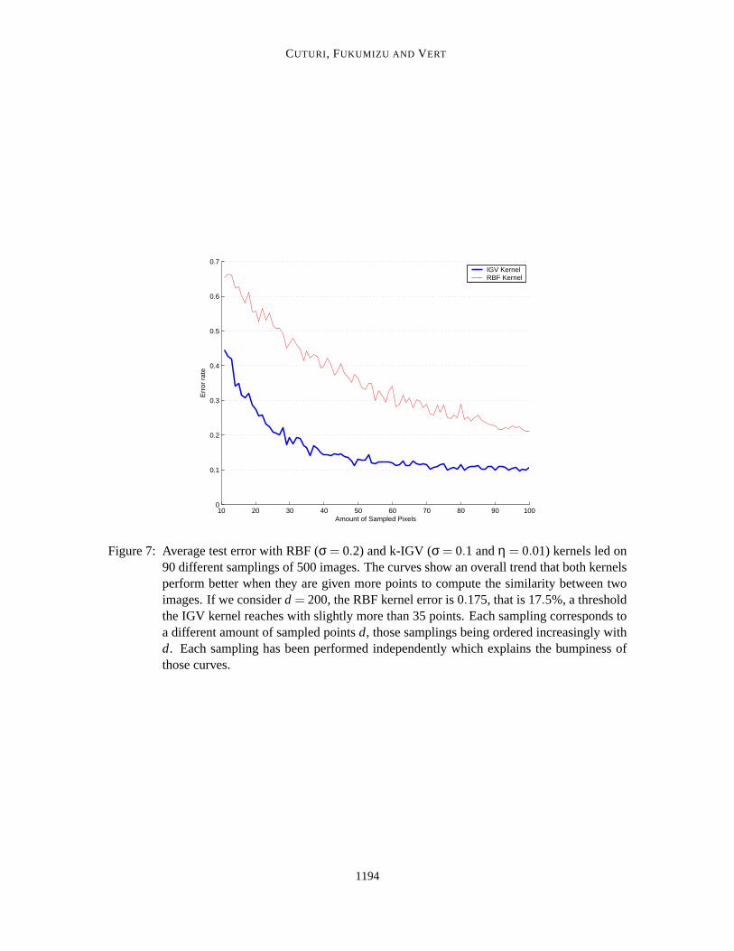
2σ2 . Since the RBF kernel is grounded on the exactoverlapping between two images we expect it to perform poorly with few pixels and significantlybetter whend grows, while we expect the k-IGV to capture more quickly the structure of the imageswith fewer pixels through the kernelκ. This is illustrated in Figure 7 where the k-IGV outperformssignificantly the RBF kernel, reaching with a sample of less than 30 points a performance the RBFkernel only reaches above 100 points. Taking roughly all black points inthe images, by settingd = 200 for instance, the RBF kernel error is still 17.5%, an error the IGV kernel reaches withroughly 35 points.

Finally, we compared the kernelized-version of the Bhattacharrya kernel (k-B) proposed in Kon-dor and Jebara (2003), the k-IGV, the polynomial kernel and the RBF kernel by using a largerdatabase of the first 1,000 images in MNIST (100 images for each of the 10 digits), selecting ran-domlyd = 40,50,60,70 and 80 points and performing the cross-validation methodology previouslydetailed. The polynomial kernel was performed seeing the images as binaryvectors of{0,1}28×28

and applying the formulakb,d(z,z′) = (z· z′ + b)d. We followed the observations of Kondor andJebara (2003) concerning parameter tuning for the k-B kernel but found out that it performed betterusing the same set of parameters used for the k-IGV. The results presented in Table 1 of the k-IGVkernel show a consistent improvement over all other kernels for this benchmark of 1000 images,under all sampling schemes.

We did not use the kernel described by Wolf and Shashua (2003) in ourexperiments becauseof its poor scaling properties for a large amount of considered points. Indeed, the kernel proposedby Wolf and Shashua (2003) takes the form of the product ofd cosines values whered is thecardinality of the considered sets of points, thus yielding negligible values in practice whend islarge as in our case. Their SVM experiments were limited to 6 or 7 points while we mostly con-sider lists of more than 40 points here. This problem of poor scaling which in practice produces adiagonal-dominant kernel led us to discarding this method in our comparison.All semigroup ker-nels presented in this paper are grounded on statistical estimation, which makes their values stableunder variable sizes of samples through renormalization, a property shared with the work of Kondorand Jebara (2003). Beyond a minimal amount of points needed to performsound estimation, thesize of submitted samples influences positively the accuracy of the k-IGV kernel. A large samplesize can lead however to computational problems since the value of the k-IGV-kernel requires notonly the computation of the centered Gram-matrixK and a few matrix multiplications, but alsothe computation of a determinant, an operation which can quickly become prohibitive since it has acomplexity ofO(d2.3) whered is the size of the considered Gram matrix. Although we did not opti-

1193


10 20 30 40 50 60 70 80 90 1000

0.1

0.2

0.3

0.4

0.5

0.6

0.7

Amount of Sampled Pixels

Err

or r

ate

IGV KernelRBF Kernel

Figure 7: Average test error with RBF (σ = 0.2) and k-IGV (σ = 0.1 andη = 0.01) kernels led on90 different samplings of 500 images. The curves show an overall trendthat both kernelsperform better when they are given more points to compute the similarity betweentwoimages. If we considerd = 200, the RBF kernel error is 0.175, that is 17.5%, a thresholdthe IGV kernel reaches with slightly more than 35 points. Each sampling corresponds toa different amount of sampled pointsd, those samplings being ordered increasingly withd. Each sampling has been performed independently which explains the bumpiness ofthose curves.

1194


mize the computations of both k-B and k-IGV kernels (by storing precomputedvalues for instanceor using numerical approximations in the computation of the determinant), this computational costin the case of a naive implementation, illustrated by the running times displayed in Table 1, remainsan issue that needs to be addressed in practical applications.

Sample SizeGaussian Polynomial k-B k-IGVσ = 0.1 b = 10;d = 4 η = 0.01;σ = 0.1 η = 0.01;σ = 0.1

40 pixels 32.2 (1) 31.3 (1.5) 19.1 (1500) 16.2 (1000)50 ” 28.5 (1) 26.3 (1.5) 17.1 (2500) 14.7 (1400)60 ” 24.5 (1) 22.0 (1.5) 15.8 (3600) 14.6 (2400)70 ” 22.2 (1) 19.5 (1.5) 15.1 (4100) 13.1 (2500)80 ” 20.3 (1) 17.4 (1.5) 14.5 (5500) 12.8 (3200)

Table 1: SVM Error rate in percents of different kernels used on a benchmark test of recognizingdigits images, where only 40 to 80 black points where sampled from the originalimages.The 1,000 images where randomly split into 3 balanced sets to perform crossvalidation (2for training and 1 for testing), the error being first averaged over 5 such splits, the wholeprocess being repeated again over 3 different random samples of points. Running timesare indicated in minutes.

9. Conclusion

We presented in this work a new family of kernels between measures. Such kernels are definedthrough prior functions which should ideally quantify the concentration of ameasure. Once sucha function is properly defined, the kernel computation goes through the evaluation of the functionon the two measures to be compared and on their mixture. As expected when dealing with con-centration of measures, two intuitive tools grounded on information theory and probability, namelyentropy and variance, prove to be useful to define such functions. Their expression is howeverstill complex in terms of computational complexity, notably for the k-IGV kernel. Computationalimprovements or numerical simplifications should be brought forward to ensure a feasible imple-mentation for large-scale tasks involving tens of thousands of objects.

An attempt to define and understand the general structure of p.d. functions on measures wasalso presented, through a representation as integrals of elementary functions known as semicharac-ters. We are investigating further theoretical properties and characterizations of both semicharactersand positive definite functions on measures. The choice of alternative priors on semicharacters topropose other meaningful kernels, with convenient properties on molecular measures for instance, isalso a subject of future research. As for practical applications, thesekernels can be naturally appliedon complex objects seen as molecular measures. We also expect to perform further experiments tomeasure the performance of semigroup kernels on a diversified sample ofchallenging tasks, in-cluding cases where the space of components is not a vector space, notably when the consideredmeasures are multinomials on a finite component space endowed with a kernel.

Acknowledgments

1195


The authors would like to thank Francis Bach and Jeremie Jakubowicz for fruitful discussions, ImreRisi Kondor for sharing his code with us, anonymous reviewers for theircomments which improvedthe quality of the paper and Xavier Dupre for his help on the MNIST database. MC acknowledgesa JSPS doctoral short-term grant which made his stay in Japan possible. KF was supported byJSPS KAKENHI 15700241 and a research grant from the Inamori Foundation. JPV is supportedby NHGRI NIH award R33 HG003070 and by the ACI “Nouvelles Interfaces des Mathematiques”of the French Ministry of Research. This work was supported in part bythe IST Programme ofthe European Community, under the PASCAL Network of Excellence, IST-2002-506778. Thispublication only reflects the authors’ views.

Appendix A : an Example of Continuous Positive Definite Function Given byNoncontinuous Semicharacters

Let X be the unit interval[0,1] hereafter. For anyt in X , a semicharacter onMb+(X ) is defined by

ρht (µ) = eµ([0,t]),

whereht(x) = I[0,t](x) is the index function of the interval[0, t]. Note thatρht is not continuous fort ∈ [0,1) by Proposition 11.

Forµ∈Mb+(X ), the functiont 7→µ([0, t)) is bounded and non-decreasing, thus, Borel-measurable,

since the discontinuous points are countable at most. A positive definite function onMb+(X ) is de-

fined by

ϕ(µ) =Z 1

0ρht (µ)dt.

This function is continuous, while it is given by the integral of noncontinuous semicharacters.

Proposition The positive definite functionϕ is continuous and exponentially bounded.

Proof Supposeµn converges toµweakly inMb+(X ). We writeFn(t) = µn([0, t]) andF(t) = µ([0, t]).

Becauseµn andµ are finite measures, the weak convergence means

Fn(t) → F(t)

for any continuous point ofF . Since the set of discontinuous points ofF is at most countable,the above convergence holds almost everywhere onX with Lebesgue measure. From the weakconvergence, we haveFn(1) → F(1), which means there existsM > 0 such that supt∈X ,n∈N Fn(t) <M. By the bounded convergence theorem, we obtain

limn→∞

ϕ(µn) = limn→∞

Z 1

0eFn(t)dt =

Z 1

0eF(t)dt = ϕ(µ).

For the exponential boundedness, by taking an absolute valueα(µ) = eµ(X), we have

|ϕ(µ)| ≤Z 1

0α(µ)dt = α(µ).

1196


References

Shotaro Akaho. A kernel method for canonical correlation analysis. InProceedings of InternationalMeeting on Psychometric Society (IMPS2001), 2001.

Shun-ichi Amari and Hiroshi Nagaoka.Methods of Information Geometry. AMS vol. 191, 2001.

Francis Bach and Michael Jordan. Kernel independent component analysis. Journal of MachineLearning Research, 3:1–48, 2002.

Christian Berg, Jens Peter Reus Christensen, and Paul Ressel.Harmonic Analysis on Semigroups.Springer-Verlag, 1984.

Alain Berlinet and Christine Thomas-Agnan.Reproducing Kernel Hilbert Spaces in Probabilityand Statistics. Kluwer Academic Publishers, 2003.

B. E. Boser, I. M. Guyon, and V. N. Vapnik. A training algorithm for optimal margin classifiers. InProceedings of the 5th annual ACM workshop on Computational Learning Theory, pages 144–152. ACM Press, 1992.

Marco Cuturi and Jean-Philippe Vert. The context-tree kernel for strings. Neural Networks, 2005.In press.

Marco Cuturi and Jean-Philippe Vert. Semigroup kernels on finite sets. InLawrence K. Saul, YairWeiss, and Leon Bottou, editors,Advances in Neural Information Processing Systems 17, pages329–336. MIT Press, Cambridge, MA, 2005.

Jean Dieudonne. Calcul Infinitesimal. Hermann, Paris, 1968.

Dominik M. Endres and Johannes E. Schindelin. A new metric for probability distributions. IEEETransactions on Information Theory, 49(7):1858–1860, 2003.

Bent Fuglede and Flemming Topsøe. Jensen-shannon divergence andhilbert space embedding. InProc. of the Internat. Symposium on Information Theory, page 31, 2004.

Kenji Fukumizu, Francis Bach, and Michael Jordan. Dimensionality reduction for supervised learn-ing with reproducing kernel hilbert spaces.Journal of Machine Learning Research, 5:73–99,2004.

M. Hein and O. Bousquet. Hilbertian metrics and positive definite kernels on probability measures.January 2005.

Tony Jebara, Risi Kondor, and Andrew Howard. Probability productkernels.Journal of MachineLearning Research, 5:819–844, 2004.

Thorsten Joachims.Learning to Classify Text Using Support Vector Machines: Methods, Theory,and Algorithms. Kluwer Academic Publishers, Dordrecht, 2002. ISBN 0-7923-7679-X.

Risi Kondor and Tony Jebara. A kernel between sets of vectors. InProceedings of the InternationalConference on Machine Learning, 2003.

1197


John Lafferty and Guy Lebanon. Information diffusion kernels. In T.G. Dietterich, S. Becker,and Z. Ghahramani, editors,Advances in Neural Information Processing Systems 14, Cambridge,MA, 2002. MIT Press.

Christina Leslie, Eleazar Eskin, and William Stafford Noble. The spectrum kernel: a string kernelfor svm protein classific ation. InProceedings of the Pacific Symposium on Biocomputing 2002,pages 564–575. World Scientific, 2002.

Christina Leslie, Eleazar Eskin, Jason Weston, and William Stafford Noble.Mismatch string ker-nels for svm protein classification. In Suzanna Becker, Sebastian Thrun, and Klaus Obermayer,editors,Advances in Neural Information Processing Systems 15, Cambridge, MA, 2003. MITPress.

Thomas Melzer, Michael Reiter, and Horst Bischof. Nonlinear feature extraction using generalizedcanonical correlation analysis. InProceedings of International Conference on Artificial NeuralNetworks (ICANN), pages 353–360, 2001.

Pedro J. Moreno, Purdy P. Ho, and Nuno Vasconcelos. A kullback-leibler divergence based ker-nel for svm classification in multimedia applications. In Sebastian Thrun, Lawrence Saul, andBernhard Scholkopf, editors,Advances in Neural Information Processing Systems 16. MIT Press,Cambridge, MA, 2004.

FerdinandOsterreicher and Igor Vajda. A new class of metric divergences on probability spacesand its applicability in statistics.Annals of the Institute of Statistical Mathematics, 55:639–653,2003.

C. R. Rao. Differential metrics in probability spaces. In S.-I. Amari, O.E. Barndorff-Nielsen,R.E. Kass, S.L. Lauritzen, and C.R. Rao, editors,Differential Geometry in Statistical Inference,Hayward,CA, 1987. Institute of Mathematical Statistics.

Walter Rudin.Fourier Analysis on Groups. John Wiley & sons, 1962.

Bernhard Scholkopf and Alexander J. Smola.Learning with Kernels: Support Vector Machines,Regularization , Optimization, and Beyond. MIT Press, Cambridge, MA, 2002.

Matthias Seeger. Covariance kernels from bayesian generative models. In T. G. Dietterich,S. Becker, and Z. Ghahramani, editors,Advances in Neural Information Processing Systems 14,pages 905–912, Cambridge, MA, 2002. MIT Press.

F. M. J. Willems, Y. M. Shtarkov, and Tj. J. Tjalkens. The context-tree weighting method: basicproperties.IEEE Transactions on Information Theory, pages 653–664, 1995.

Lior Wolf and Amnon Shashua. Learning over sets using kernel principal angles.Journal of Ma-chine Learning Research, 4:913–931, 2003.

1198

Semigroup Kernels on Measures

Documents

Transcript of Semigroup Kernels on Measures