Semiempirical Method for Prediction of …...Semiempirical Method for Prediction of Aerodynamic...
87
I 1 ~~~ ~ NASA Technical Memorandum 4009 Semiempirical Method for Prediction of Aerodynamic Forces and Moments on a Steadily Spinning Light Airplane Bandu N. Pamadi Vigyan Researcb Associates, lnc. Hampton, Virginia Lawrence W. Taylor, Jr. Langley Researcb Center Hampton, Virginia National Aeronautics and Space Administration 1 Scientific and Technical Information Division 1987 https://ntrs.nasa.gov/search.jsp?R=19880003074 2020-06-25T19:18:25+00:00Z
Transcript of Semiempirical Method for Prediction of …...Semiempirical Method for Prediction of Aerodynamic...
I
1
~~~ ~ ~~~~ ~~~
NASA Technical Memorandum 4009
Semiempirical Method for Prediction of Aerodynamic Forces and Moments on a Steadily Spinning Light Airplane
Bandu N. Pamadi
Vigyan Researcb Associates, lnc. Hampton, Virginia
Lawrence W. Taylor, Jr.
Langley Researcb Center Hampton, Virginia
National Aeronautics and Space Administration
1
Scientific and Technical Information Division
1987
https://ntrs.nasa.gov/search.jsp?R=19880003074 2020-06-25T19:18:25+00:00Z
Contents
Summary . . . . . . . . . . . . . . . . . . . . . . . . . . . . . . . . . . 1
Symbols . . . . . . . . . . . . . . . . . . . . . . . . . . . . . . . . . . . 2
Analysis . . . . . . . . . . . . . . . . . . . . . . . . . . . . . . . . . . . 4
Strip theory calculations . . . . . . . . . . . . . . . . . . . . . . . . . . 4 Effect of angular velocity on wing . . . . . . . . . . . . . . . . . . . . . . Studies at low angles of attack . . . . . . . . . . . . . . . . . . . . . . . 6 Studies at high angles of attack . . . . . . . . . . . . . . . . . . . . . . .
Introduction . . . . . . . . . . . . . . . . . . . . . . . . . . . . . . . . . 1
Wing Contribution . . . . . . . . . . . . . . . . . . . . . . . . . . . . . 4
5
6 Body Contribution . . . . . . . . . . . .
Body at angle of attack . . . . . . . . . Body in sideslip . . . . . . . . . . . . . Combined angles of attack and sideslip . . Strip theory calculations . . . . . . . . . Rotational flow effects . . . . . . . . . .
Horizontal Tail Contribution . . . . . . . . Strip theory calculations . . . . . . . . . Rotational flow effects . . . . . . . . . .
Vertical Tail Contribution . . . . . . . . . Shielding effect . . . . . . . . . . . . . Modeling of two-dimensional flat-plate wake Calculation of aerodynamic coefficients . . Secondary flow effects . . . . . . . . . .
. . . . . . . . . . . . . . . . 7
. . . . . . . . . . . . . . . . 7 . . . . . . . . . . . . . . . . . 8 . . . . . . . . . . . . . . . . . 8 . . . . . . . . . . . . . . . . . 8 . . . . . . . . . . . . . . . . . 9 . . . . . . . . . . . . . . . . . 9 . . . . . . . . . . . . . . . . . 9 . . . . . . . . . . . . . . . . . 10 . . . . . . . . . . . . . . . . 110 . . . . . . . . . . . . . . . . . 10 . . . . . . . . . . . . . . . . . 10 . . . . . . . . . . . . . . . . . 11 . . . . . . . . . . . . . . . . . 11
Total Airplane . . . . . . . . . . . . . . . . . . . . . . . . . . . . . . . 12
Application . . . . . . . . . . . . . . . . . . . . . . . . . . . . . . . . . 13 InputData . . . . . . . . . . . . . . . . . . . . . . . . . . . . . . . . 14
Wing . . . . . . . . . . . . . . . . . . . . . . . . . . . . . . . . . . 14 Body . . . . . . . . . . . . . . . . . . . . . . . . . . . . . . . . . . 14 Horizontal tail . . . . . . . . . . . . . . . . . . . . . . . . . . . . . 15 Vertical tail . . . . . . . . . . . . . . . . . . . . . . . . . . . . . . 15
Presentation of Results . . . . . . . . . . . . . . . . . . . . . . . . . . . 15
Discussion . . . . . . . . . . . . . . . . . . . . . . . . . . . . . . . . . . 15 Static Aerodynamic Characteristics
Body . . . . . . . . . . . . CL . . . . . . . . . . . . . c, . . . . . . . . . . . . . c y . . . . . . . . . . . . . c, . . . . . . . . . . . . . BW configuration . . . . . . . BHV configuration . . . . . .
. . . . . . . . . . . . . . . . . . . . . . 15
. . . . . . . . . . . . . . . . . . . . . . 15
. . . . . . . . . . . . . . . . . . . . . . 15
. . . . . . . . . . . . . . . . . . . . . . 15
. . . . . . . . . . . . . . . . . . . . . 15
. . . . . . . . . . . . . . . . . . . . . . 16
. . . . . . . . . . . . . . . . . . . . . 16
. . . . . . . . . . . . . . . . . . . . . . 16 Rotary Aerodynamic Characteristics . . . . . . . . . . . . . . . . . . . . . 16
Body (B) configuration . . . . . . . . . . . . . . . . . . . . . . . . . . 16 BW configuration . . . . . . . . . . . . . . . . . . . . . . . . . . . . 16 BH configuration . . . . . . . . . . . . . . . . . . . . . . . . . . . . . 16 BV configuration . . . . . . . . . . . . . . . . . . . . . . . . . . . . . 16 BWH configuration . . . . . . . . . . . . . . . . . . . . . . . . . . . 16 BWV configuration . . . . . . . . . . . . . . . . . . . . . . . . . . . 16
BHV configuration . . . . . . . . . . . . . . . . . . . . . . . . . . . . 17 BWHV configuration . . . . . . . . . . . . . . . . . . . . . . . . . . 17
Concluding Remarks . . . . . . . . . . . . . . . . . . . . . . . . . . . . . 17
References . . . . . . . . . . . . . . . . . . . . . . . . . . . . . . . . . . 18
Prediction of Equilibrium Spin Modes . . . . . . . . . . . . . . . . . . . . . 17
iv
List of Tables Table I. Dimensional Characteristics of Full-scale Model A Airplane
Table 11. Side-Force Coefficients of Airplane Components
Table 111. Normal-Force Coefficients of Airplane Components
Table IV. Yawing-Moment Coefficients of Airplane Components
Table V. Rolling-Moment Coefficients of Airplane Components
Table VI. Pitching-Moment Coefficients of Airplane Components
V
List of Figures Figure 1. Schematic diagram of steadily rotating airplane model in spin tunnel.
Figure 2. Schematic diagram showing strip parameters of wing and body of rotating airplane.
Figure 3. Variation of section lift and drag coefficients on rotating propeller. (From Himmelskamp, ref. 9.)
Figure 4. Strip theory calculations for Himmelskamp’s rotating propeller (ref. 9).
Figure 5. Comparison of strip theory calculations for normal-force coefficient with rotary balance test data. (From ref. 13.)
Figure 6. Comparison of McCormick’s strip theory calculations for normal-force coefficient incorporating radial pressure gradient term (ref. 13) with rotary balance test data (ref. 11).
Figure 7. Comparison of calculated rolling-moment coefficient based on strip theory and radial pressure gradient correction (ref. 13) with rotary balance test data (ref. 11).
Figure 8. Aerodynamic characteristics of two-dimensional square cylinders (ref. 24).
Figure 9. Static body at angles of attack and sideslip.
Figure 10. Wing-tail flow interactions.
Figure 11. Schematic diagram showing shielding of vertical tail in right spin.
Figure 12. Modeling of shielded area of vertical tail in spin.
Figure 13. Schematic diagram of impingement of wake flow over vertical tail.
Figure 14. Schematic illustration of secondary flow effects over vertical tail in right spin.
Figure 15. Schematic sketch of idealized impinging flow (ref. 32).
Figure 16. Spin research airplane (full scale). Model A with tail 3.
Figure 17. Tail configurations.
Figure 18. Input static aerodynamic data for wing and horizontal tail. N R ~ = 0.288 x lo6.
Figure 19. Cross-flow angles over body.
Figure 20. Geometry of body of model A airplane.
Figure 21. Actual and assumed cross-sectional areas of body.
Figure 22. Idealized cross-sectional shape of body.
Figure 23. Correlation of side-force data (ref. 10). N R ~ = 0.288 x lo6.
Figure 24. Schematic sketch of flow patterns.
Figure 25. Interactions of wing wake and horizontal tail.
Figure 26. Side-force coefficients for unshielded vertical tail of low aspect ratio.
Figure 27. Graphical evaluation of shielded area of vertical tail at various angles of attack (tail 4).
Figure 28. Variation of shielded area with angle of attack.
Figure 29. Static longitudinal aerodynamic coefficients of body of model A airplane. N R ~ = 0.288 x lo6.
Figure 30. Static side-force characteristics of body of model A airplane.
Figure 31. Static yawing-moment characteristics of body of model A airplane.
vi
, Figure 32. Comparison of static side-force and yawing-moment coefficients of body-alone and wing-body configurations.
Figure 33. Static side-force and yawing-moment coefficients of BHV configuration.
Figure 34. Rotary aerodynamic characteristics of body (B) configuration.
Figure 35. Rotary aerodynamic characteristics of BW configuration.
Figure 36. Rotary aerodynamic characteristics of BH configuration.
Figure 37. Rotary aerodynamic characteristics of BV configuration.
Figure 38. Rotary aerodynamic characteristics of BWH configuration with tail 3.
Figure 39. Rotary aerodynamic characteristics of BWV Configuration.
Figure 40. Rotary aerodynamic characteristics of BHV configuration with tail 3.
Figure 41. Rotary aerodynamic characteristics of BHV configuration with tail 4.
Figure 42. Rotary aerodynamic characteristics of BWHV configuration with tail 3.
Figure 43. Rotary aerodynamic characteristics of BWHV configuration with tail 4.
Figure 44. Rotary aerodynamic characteristics of BWHV configuration with tail 5.
Figure 45. Rotary aerodynamic characteristics of model A airplane with tail 3 at moderately flat spin attitude. a = 50'.
Figure 46. Rotary aerodynamic characteristics of model A airplane with tail 3 at flat spin attitude. a = 80'.
Figure 47. Rotary aerodynamic characteristics of model A airplane with tail 4 at steep spin attitude. a = 35'.
Figure 48. Rotary aerodynamic characteristics of model A airplane with tail 4 at flat spin attitude. a = 80'.
Figure 49. Rotary aerodynamic characteristics of model A airplane with tail 5 at moderately steep spin attitude. a = 40'.
vii
Summary Introduction
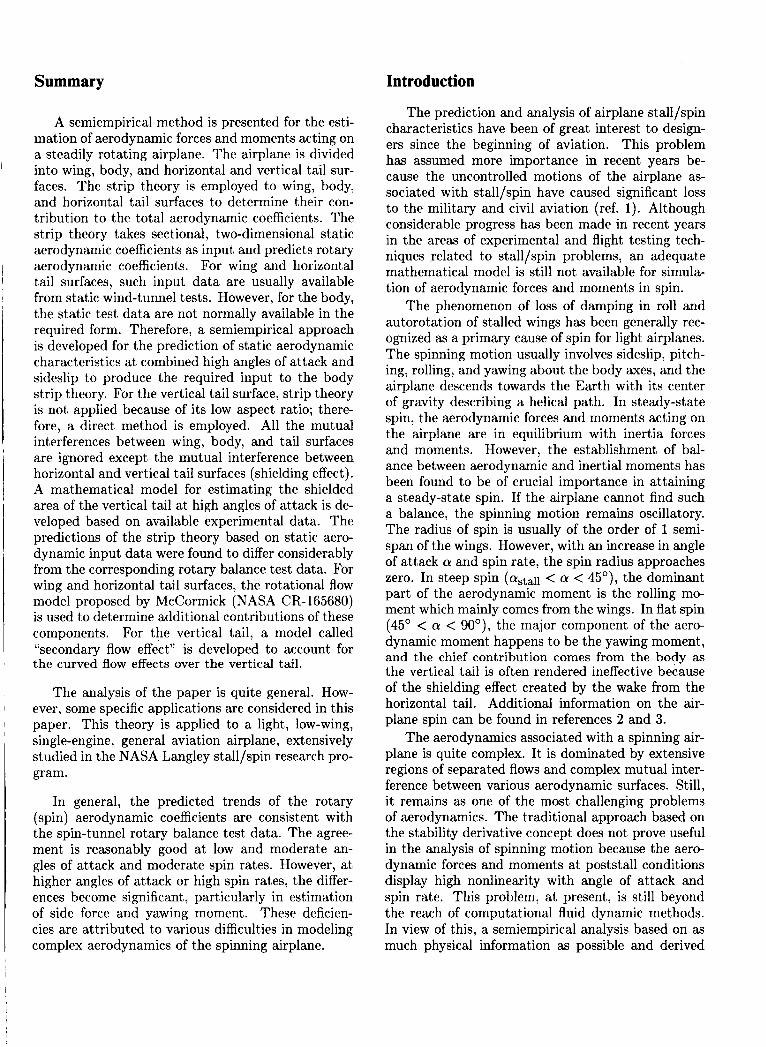
A semiempirical method is presented for the esti- mation of aerodynamic forces and moments acting on a steadily rotating airplane. The airplane is divided into wing, body, and horizontal and vertical tail sur- faces. The strip theory is employed to wing, body, and horizontal tail surfaces to determine their con- tribution to the total aerodynamic coefficients. The strip theory takes sectional, two-dimensional static aerodynamic coefficients as input and predicts rotary aerodynamic coefficients. For wing and horizontal tail surfaces, such input data are usually available from static wind-tunnel tests. However, for the body, the static test data are not normally available in the required form. Therefore, a semiempirical approach is developed for the prediction of static aerodynamic characteristics at combined high angles of attack and sideslip to produce the required input to the body strip theory. For the vertical tail surface, strip theory is not applied because of its low aspect ratio; there- fore, a direct method is employed. All the mutual interferences between wing, body, and tail surfaces are ignored except the mutual interference between horizontal and vertical tail surfaces (shielding effect). A mathematical model for estimating the shielded area of the vertical tail at high angles of attack is de- veloped based on available experimental data. The predictions of the strip theory based on static aero- dynamic input data were found to differ considerably from the corresponding rotary balance test data. For wing and horizontal tail surfaces, the rotational flow model proposed by McCormick (NASA CR-165680) is used to determine additional contributions of these components. For the vertical tail, a model called ''secondary flow effect'' is developed to account for the curved flow effects over the vertical tail.
The analysis of the paper is quite general. How- ever, some specific applications are considered in this paper. This theory is applied to a light, low-wing, single-engine, general aviation airplane, extensively studied in the NASA Langley stall/spin research pro- gram.
In general, the predicted trends of the rotary (spin) aerodynamic coefficients are consistent with the spin-tunnel rotary balance test data. The agree- ment is reasonably good at low and moderate an- gles of attack and moderate spin rates. However, at higher angles of attack or high spin rates, the differ- ences become significant, particularly in estimation of side force and yawing moment. These deficien- cies are attributed to various difficulties in modeling complex aerodynamics of the spinning airplane.
The prediction and analysis of airplane stall/spin characteristics have been of great interest to design- ers since the beginning of aviation. This problem has assumed more importance in recent years be- cause the uncontrolled motions of the airplane as- sociated with stall/spin have caused significant loss to the military and civil aviation (ref. 1). Although considerable progress has been made in recent years in the areas of experimental and flight testing tech- niques related to stall/spin problems, an adequate mathematical model is still not available for simula- tion of aerodynamic forces and moments in spin.
The phenomenon of loss of damping in roll and autorotation of stalled wings has been generally rec- ognized as a primary cause of spin for light airplanes. The spinning motion usually involves sideslip, pitch- ing, rolling, and yawing about the body axes, and the airplane descends towards the Earth with its center of gravity describing a helical path. In steady-state spin, the aerodynamic forces and moments acting on the airplane are in equilibrium with inertia forces and moments. However, the establishment of bal- ance between aerodynamic and inertial moments has been found to be of crucial importance in attaining a steady-state spin. If the airplane cannot find such a balance, the spinning motion remains oscillatory. The radius of spin is usually of the order of 1 semi- span of the wings. However, with an increase in angle of attack a and spin rate, the spin radius approaches zero. In steep spin (astall < a < 45'), the dominant part of the aerodynamic moment is the rolling mo- ment which mainly comes from the wings. In flat spin (45' < Q < go'), the major component of the aero- dynamic moment happens to be the yawing moment, and the chief contribution comes from the body as the vertical tail is often rendered ineffective because of the shielding effect created by the wake from the horizontal tail. Additional information on the air- plane spin can be found in references 2 and 3.
The aerodynamics associated with a spinning air- plane is quite complex. It is dominated by extensive regions of separated flows and complex mutual inter- ference between various aerodynamic surfaces. Still, it remains as one of the most challenging problems of aerodynamics. The traditional approach based on the stability derivative concept does not prove useful in the analysis of spinning motion because the aero- dynamic forces and moments at poststall conditions display high nonlinearity with angle of attack and spin rate. This problem, at present, is still beyond the reach of computational fluid dynamic methods. In view of this, a semiempirical analysis based on as much physical information as possible and derived
from experimental work can play an important role in the theoretical analysis of airplane spin.
Glauert (ref. 3), Gates and Bryant (ref. 4), and Wykes, Casteel, and Collins (ref. 5) employed strip theory to estimate the aerodynamic characteristics of a steadily spinning airplane. The strip theory takes static aerodynamic data as input and predicts the rotary aerodynamic coefficients. These studies were limited to the analysis of steep spins. The problem of flat spins, where both the angle of attack and spin rates can be quite high, was not given much atten-
I tion. Nonavailability of an adequate aerodynamic mathematical model led to the development of the spin-tunnel rotary balance apparatus for generating the pertinent aerodynamic test data (ref. 6). By in- corporating the spin-tunnel rotary balance aerody-
tions of motion, it has been demonstrated that the steady-state spins can usually be predicted (refs. 7 and 8). Thus, the experimental data base generated by rotary balance tests has played a very useful role in understanding the stall spin problems. On the other hand, for a spinning airplane, the experimen- tal investigations dealing with flow visualization and pressure measurements similar to those carried out for rotating propellers (ref. 9) and which could pro- vide insight to develop a comprehensive theory are
In the present study, an effort has been made to estimate the aerodynamic forces and moments acting on a light spinning airplane. Here, the airplane is considered to be steadily rotating about a vertical axis analogous to a model undergoing spin-tunnel
in as closely as possible with the rotary balance test data. Also, this condition approximates quite well an airplane in a steady-state spinning flight. Angles of attack up to 90’ and reduced spin rates up to 1.0
The airplane model is considered to be divided into wing, body, horizontal and vertical tail surfaces. The effect of power is ignored. The strip theory used for wing and horizontal tail surfaces is based on the input of sectional, two-dimensional static wind- tunnel test data (ref. 10) and is similar to the meth- ods used in earlier studies (refs. 3 and 4). How- ever, for the body, the static wind-tunnel test data in sectional coefficient form are not usually avail- able. Therefore, a semiempirical approach is devel- oped to predict the static aerodynamic characteris- tics at combined high angles of attack and sideslip to generate the required input to body theory. All the interference effects between wing, body, and tail surfaces are ignored except the mutual interference between horizontal and vertical tail surfaces (shield-
I
I
~
I
l
namic test data into the six-degree-of-freedom equa-
I
I
I almost nonexistent.
, rotary balance tests so that the present theory ties I
I I
are considered in the present analysis.
ing effect). A procedure for estimating the shielded area of the vertical tail is developed based on experi- mental data and is incorporated in the calculation of vertical tail aerodynamic characteristics.
The predictions of the strip theory based on the static aerodynamic input data were found to differ considerably from the corresponding rotary balance test data (refs. 11 and 12). This discrepancy is at- tributed to the presence of curved or rotational fluid flow. Herein the term “rotational flow” is used to refer to the curved nature of the flow due to an- gular velocity R. The simple strip theory accounts only for the kinematics associated with angular veloc- ity R and has no mechanism to handle the physical aspects of the flow pattern. A brief description of the flow field over rotating airplane surfaces is pre- sented based on available information in the litera- ture. For wing and horizontal tail surfaces, the rota- tional flow model proposed by McCormick (ref. 13) is employed to determine additional contributions of these components. The rotational flow effects are ig- nored for the body. For the vertical tail, a secondary flow model is proposed to account for its curved flow effects.
The strip theory is applied to a light, single- engine, low wing general aviation airplane which has been extensively studied as model A in references 10, 11, 12, 14, and 15. We have presented calculations for the basic configuration of the model A airplane of references 10, 11, 12, 14, and 15, whose tail con- figuration is designated as tail 4, and two other tail configurations (3 and 5). The presentation of results follows the pattern of spin-tunnel rotary balance test data of references 10 through 12. The nomencla- ture adopted is also similar to that used in these references.
For application of the present method to other light airplane configurations, it is necessary to have the input empirical data in the form similar to that discussed.
Some partial results of this investigation have been presented by the authors to recent conferences (refs. 16 and 17). An extension of the strip theory approach to wings of arbitrary planform is presented in reference 18.
Symbols A axial force AR aspect ratio bH horizontal tail span
bh
bV vertical tail span bW wing span
local width of body cross section
2
axial-force coefficient, Axial force 3PU&SW
drag coefficient
lift coefficient, Lift 3PU%SW
rolling-moment coefficient, Rolling moment about cg
pitching-moment coefficient,
3 PU% SW bw
Pitching moment about cg 3PU%SWFW
normal-force coefficient, Normal force
yawing-moment coefficient, Yawing moment about cg
two-dimensional axial-force coefficient
axial-force coefficient of two- dimensional square section
;Pu&sw
;PU%Swbw
side-force coefficient, Side Force $PU%SW
side-force coefficient of unshielded vertical tail
side-force coefficient of idealized two- dimensional body cross section of model A airplane
side-force coefficient of two- dimensional square cross section
local chord
drag coefficient of circular cylinder
chord of flat plate
wing mean geometric chord
drag force
maximum width of flat-plate wake
vertical tail side force
vertical distance between X-axis and centroid of unshielded area of vertical tail
apparent mass coefficients of body
lift force
length of body
horizontal tail length, distance be- tween 0.25 mean aerodynamic chord of horizontal tail and airplane center of gravity
vertical tail length, distance between 0.25 mean aerodynamic chord of vertical tail and airplane center of gravity
normal force Reynolds number pressure stagnation pressure static pressure pressure in wake local dynamic pressure free-stream dynamic pressure,
spin radius radius corner radius of square cross section radius of impinging airstream
streamwise coordinate of stagnation streamline in secondary flow over vertical tail
tPU&
area cross-sectional area of body maximum cross-sectional area of body
shielded area effective vertical tail cross-sectional area
local velocity velocity along stagnation streamline
free-stream velocity volume of body axis system coordinate system attached to body with origin at center of gravity
center-of-gravity location, measured from nose of body = %
center of pressure of wing measured from leading edge and expressed in terms of chord
(fig. 15)
C
3
CY
ae
P A E
rlH
%tall
rlV
d
flH
x
AH
P
4 4 c W
R
angle of attack
local angle of attack
sideslip angle
elemental quantity (strip)
correction factor for three-dimensional effects over body
horizontal tail efficiency, m/qW
spanwise extent of stall over wing or horizontal tail, w- vertical tail efficiency, E = tan-' 3 = tan-' %
= tan-' 2 density
cross-flow angle, tan-1
cross-flow angle when C y = 0
reduced spin rate, positive for right spin and negative for left spin (as viewed from top), Rb/2U
angular velocity about spin axis, positive for right spin and negative for left spin (as viewed from top)
Subscripts:
L left
e strip or local
max maximum
min minimum
R right
stall
Superscript: I
condition or parameter at stall
parameter in rotational or secondary flow effect
Abbreviations (also used as subscripts):
B body (fuselage)
cg center of gravity
H horizontal tail
V vertical tail
4
w wing 2-D two-dimensional
Analysis Let us consider an airplane model, mounted on
a rotary balance apparatus in the spin tunnel and steadily rotating at a constant angular velocity R about the spin axis, which is vertical. A schematic sketch of this configuration is shown in figure 1. For the purpose of this analysis, the following assump tions are introduced, mainly because we intend to tie the present theory as closely as possible to the test conditions employed in the rotary balance tests (refs. 11 and 12), which could be generally different from those encountered in actual steady-state spin of the free airplane:
1. The spin axis passes through the model cen- ter of gravity so that the spin radius R and sideslip at center of gravity are zero
2. The Y-axis of the airplane lies in the horizon- tal plane so that the bank angle is zero
3. The effect of power is ignored and the model configuration without propeller is considered in the analysis
4. The control surface deflections are zero; in the present analysis, the dihedral effects of wing and horizontal tail are ignored and the mu- tual aerodynamic interferences between vari- ous airplane components are ignored except the interference between horizontal and verti- cal tail surfaces (shielding effect); however, it is possible that some of the interference effects not considered herein could be significant, as discussed later, and need proper modeling
5. Difference between tunnel test and flight Reynolds number is ignored
In strip theory approach, the surface (say wing) is usually divided into a number of strips. The force on each strip is assumed to be the same a5 it would be were the surface moving with an equivalent linear velocity, that is, the vector sum of all the linear velocities at that strip. For a rectangular wing with strips oriented normal to the Y-axis (fig. 2), this equivalent velocity is equal to U + Ry. The strip theory approach used for wings and horizontal tails is similar to that employed by Glauert (ref. 3).
Wing Contribution
Strip theory calculations. Consider the airplane model to be rotating in a clockwise (positive) direc- tion as viewed from the top. The effect of the angular velocity in spin R is to induce, at any spanwise loca- tion y, a velocity component equal to Ry as indicated
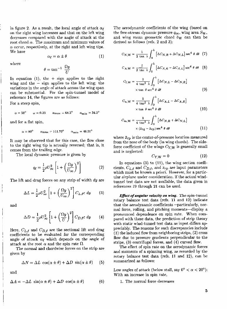
in figure 2. As a result, the local angle of attack on the right wing increases and that on the left wing decreases compared with the angle of attack at the root chord a. The maximum and minimum values of a occur, respectively, at the right and left wing tips. We have
a e = Q & 0 (1)
where 1 R y
U 13 = tan-
In equation (l), the + sign applies to the right wing and the - sign applies to the left wing; the variations in the angle of attack across the wing span can be substantial. For the spin-tunnel model of reference 14, the figures are as follows: For a steep spin,
and for a flat spin,
It may be observed that for this case, the flow close to the right wing tip is actually reversed; that is, it comes from the trailing edge.
The local dynamic pressure is given by
The lift and drag forces on any strip of width dy are
and
AD = ApU& 2 [ 1 + ( $)2] C D , ~ C dy (4)
Here, CL,e and Co,e are the sectional lift and drag coefficients to be evaluated for the corresponding angle of attack a! which depends on the angle of attack at the root a and the spin rate fl.
The normal and chordwise forces on the strip are given by
AN = AL cos(a f 19) + AD sin(@ f 0) (5)
and
AA = -AL sin(a f e) + AD cos(a f 0) (6)
The aerodynamic coefficients of the wing (based on the free-stream dynamic pressure goo, wing area Sw , and wing mean geometric chord Cw can then be derived as follows (refs. 2 and 3):
x tan 6 sec4 9 d6 (9)
x (zCg - zCp) sec4 6 d6 (11)
where Zcp is the center-of-pressure location measured from the nose of the body (in wing chords). The side- force coefficient of the wings Cy,w is generally small and is neglected:
CY,, = 0 (12) In equations (3) to (11), the wing section coeffi-
cients, CL,e and c D , [ , and Z,, are input parameters which must be known a priori. However, for a partic- ular airplane under consideration, if the actual wind- tunnel test data are not available, the data given in references 19 through 21 can be used.
Eflect of angular velocity on wing. The spin-tunnel rotary balance test data (refs. 11 and 12) indicate that the aerodynamic coefficients-particularly, nor- mal force, rolling, and pitching moments-display a pronounced dependence on spin rate. When com- pared with these data, the prediction of strip theory with static wind-tunnel test data as input differs ap- preciably. The reasons for such discrepancies include (1) the induced flow from neighboring strips, (2) cross flow due to pressure gradients perpendicular to the strips, (3) centrifugal forces, and (4) curved flow.
The effect of spin rate on the aerodynamic forces and moments of a spinning wing, as recorded by the rotary balance test data (refs. 11 and 12), can be summarized as follows:
Low angles of attack (below stall, say 0' < a < 20'): With an increase in spin rate,
1. The normal force decreases
5
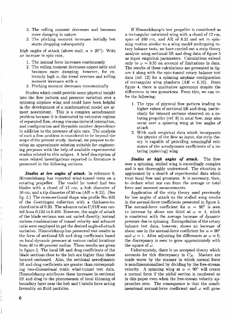
2. The rolling moment decreases and becomes
3. The pitching moment increases initially but
High angles of attack (above stall, Q > 20'): With an increase in spin rate,
more damping in nature
starts dropping subsequently
1. The normal force increases continuously 2. The rolling moment decreases appreciably and
becomes more damping; however, for ex- tremely high a, the trend reverses and rolling moment increases with Q
3. Pitching moment decreases monotonically Studies which could provide some physical insight
into the flow pattern and pressure variation over a spinning airplane wing and could have been helpful in the development of a mathematical model are al- most nonexistent. This is a complex aerodynamic problem because it is dominated by extensive regions of separated flow, strong viscous-inviscid interaction, and configuration and Reynolds number dependence in addition to the presence of spin rate. The analysis of such a flow problem is considered to be beyond the scope of the present study. Instead, we propose to de- velop an approximate solution suitable for engineer- ing purposes with the help of available experimental studies related to this subject. A brief description of some related investigations reported in literature is presented in the following sections.
Studies at low angles of attack. In reference 9, Himmelskamp has reported wind-tunnel tests on a rotating propeller. The model he tested had two blades with a chord of 12 cm, a hub diameter of 10 cm, and a tip diameter of 50 cm (AR = 8.33). (See fig. 3.) The cross-sectional shape was profile No. 625 of the Goettingen collection with a thickness-to- chord ratio of 0.20. The advance ratio UIRR was var- ied from 0.124 to 0.459. However, the angle of attack of the blade sections was not varied directly; instead various combinations of tunnel velocity and advance ratio were employed to get the desired angle-of-attack variation. Himmelskamp has presented test results in the form of sectional lift and drag coefficients based on local dynamic pressure at various radial locations from 40 to 80 percent radius. These results are given in figure 3. The local lift and drag coefficients of the blade sections close to the hub are higher than those located outboard. Also, the sectional aerodynamic lift and drag coefficients are greater than correspond- ing two-dimensional static wind-tunnel test data. Himmelskamp attributes these increases in sectional lift and drag to the phenomenon of local thinning of boundary layer near the hub and Coriolis force acting favorably on fluid particles.
If Himmelskamp's test propeller is considered as a rectangular untwisted wing with a chord of 12 cm, span of 100 cm, and AR of 8.33 and set in spin- ning motion similar to a wing model undergoing ro- tary balance tests, we have carried out a strip theory analysis using sectional lift and drag data of figure 3 as input empirical parameters. Calculations extend only to w = 0.35 on account of limitations in data. The results of these calculations are presented in fig- ure 4 along with the spin-tunnel rotary balance test data (ref. 12) for a spinning airplane configuration of rectangular wing planform (AR = 6.10). From figure 4, there is qualitative agreement despite the differences in two geometries. From this, we can in- fer the following:
1. The type of physical flow pattern leading to higher values of sectional lift and drag, partic- ularly for inboard sections observed on a ro- tating propeller (ref. 9) in axial flow, may also occur over a spinning wing at low angles of attack
2. With such empirical data which incorporate the physics of the flow as input, the strip the- ory is capable of providing meaningful esti- mates of the aerodynamic coefficients of a ro- tating (spinning) wing
Studies ut high angles of attack. The flow over a spinning, stalled wing is exceedingly complex and is not thoroughly understood. The situation is aggravated by a dearth of experimental data which treat local flow and pressures. It is necessary, then, to deduce what one can from the average or total force and moment measurements.
Application of the strip theory used previously for low angles of attack to the stalled wing results in the normal-force coefficients presented in figure 5. The normal-force coefficient for a = 90' is seen to increase by about one third at w = 1, which is consistent with the average increase of dynamic pressure due to spinning. Extrapolation of the rotary balance test data, however, shows an increase of about one in the normal-force coefficient for a = 90' and w = 1. After adjusting for differences at w = 0, the discrepancy is seen to grow approximately with the square of w .
Unfortunately, there is no accepted theory which accounts for this discrepancy in CN. Matters are made worse by the manner in which normal force is nondimensionalized by dividing by the free-stream velocity. A spinning wing at a = 90' will create a normal force if the airfoil section is cambered as in this paper even when the free-stream velocity ap- proaches zero. The consequence is that the nondi- mensional normal-force coefficient and w will grow
6
without bound as U approaches zero. Propeller char- acteristics are usually nondimensionalized by using the tip velocity which avoids this singularity.
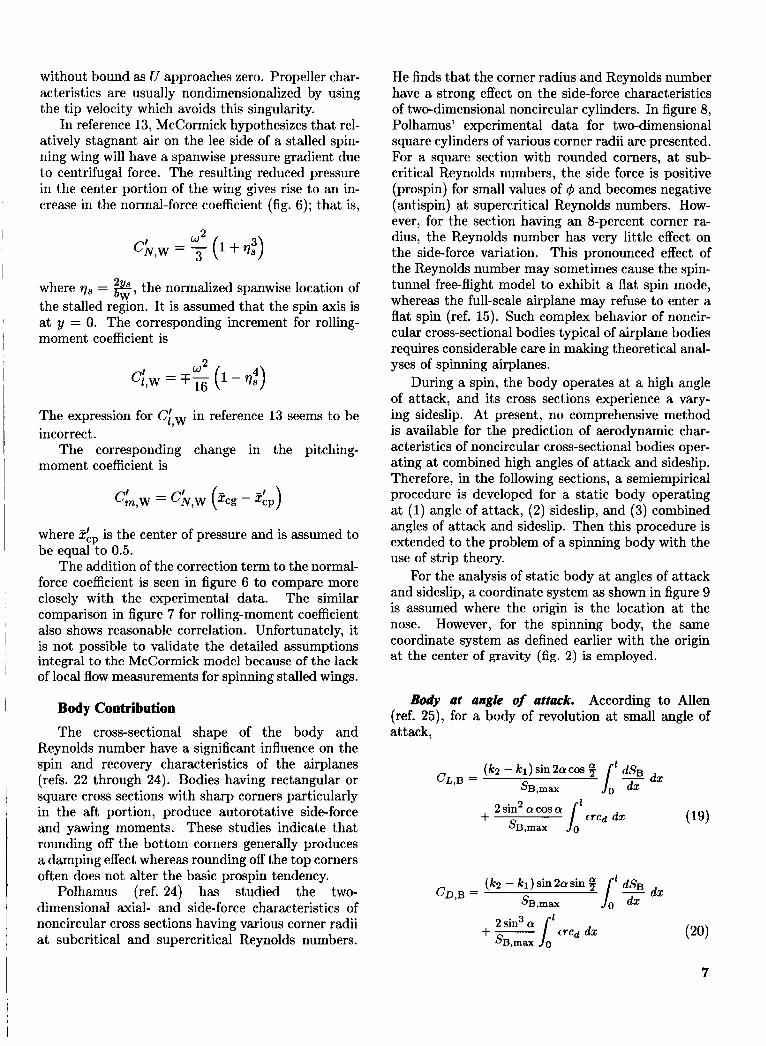
In reference 13, McCormick hypothesizes that rel- atively stagnant air on the lee side of a stalled spin- ning wing will have a spanwise pressure gradient due to centrifugal force. The resulting reduced pressure in the center portion of the wing gives rise to an in- crease in the normal-force coefficient (fig. 6); that is,
where qs = p, the normalized spanwise location of the stalled region. It is assumed that the spin axis is at y = 0. The corresponding increment for rolling- moment coefficient is
W
The expression for Ci,w in reference 13 seems to be incorrect.
The corresponding change in the pitching- moment coefficient is
where 3Lp is the center of pressure and is assumed to be equal to 0.5.
The addition of the correction term to the normal- force coefficient is seen in figure 6 to compare more closely with the experimental data. The similar comparison in figure 7 for rolling-moment coefficient also shows reasonable correlation. Unfortunately, it is not possible to validate the detailed assumptions integral to the McCormick model because of the lack of local flow measurements for spinning stalled wings.
Body Contribution The cross-sectional shape of the body and
Reynolds number have a significant influence on the spin and recovery characteristics of the airplanes (refs. 22 through 24). Bodies having rectangular or square cross sections with sharp corners particularly in the aft portion, produce autorotative side-force and yawing moments. These studies indicate that rounding off the bottom corners generally produces a damping effect whereas rounding off the top corners often does not alter the basic prospin tendency.
Polhamus (ref. 24) has studied the two- dimensional axial- and side-force characteristics of noncircular cross sections having various corner radii at subcritical and supercritical Reynolds numbers.
He finds that the corner radius and Reynolds number have a strong effect on the side-force characteristics of two-dimensional noncircular cylinders. In figure 8, Polhamus’ experimental data for two-dimensional square cylinders of various corner radii are presented. For a square section with rounded corners, at sub- critical Reynolds numbers, the side force is positive (prospin) for small values of 4 and becomes negative (antispin) at supercritical Reynolds numbers. How- ever, for the section having an 8-percent corner ra- dius, the Reynolds number has very little effect on the side-force variation. This pronounced effect of the Reynolds number may sometimes cause the spin- tunnel free-flight model to exhibit a flat spin mode, whereas the full-scale airplane may refuse to enter a flat spin (ref. 15). Such complex behavior of noncir- cular cross-sectional bodies typical of airplane bodies requires considerable care in making theoretical anal- yses of spinning airplanes.
During a spin, the body operates at a high angle of attack, and its cross sections experience a vary- ing sideslip. At present, no comprehensive method is available for the prediction of aerodynamic char- acteristics of noncircular cross-sectional bodies oper- ating at combined high angles of attack and sideslip. Therefore, in the following sections, a semiempirical procedure is developed for a static body operating at (1) angle of attack, (2) sideslip, and (3) combined angles of attack and sideslip. Then this procedure is extended to the problem of a spinning body with the use of strip theory.
For the analysis of static body at angles of attack and sideslip, a coordinate system as shown in figure 9 is assumed where the origin is the location at the nose. However, for the spinning body, the same coordinate system as defined earlier with the origin at the center of gravity (fig. 2) is employed.
Body at angle of attack. According to Allen (ref. 25), for a body of revolution at small angle of attack,
(k2 - kl ) sin 2 a cos 4 J,’* dx CL,B =
+ dx SB,max
2 sin2 a cos a SB,max
€rCd dx J,’
(k2 - k l ) s i n 2 a s i n 4 dSB CD,B =
SB,max
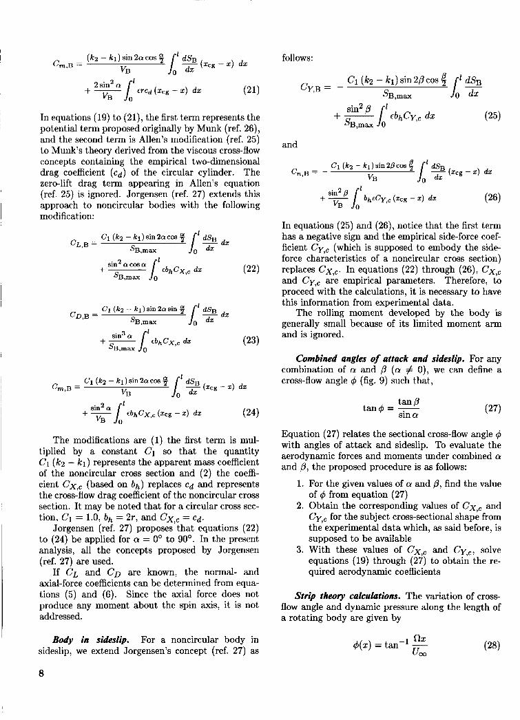
follows: (k2 - kl) sin 2 a cos 9 VB
I' % (xcg - x) dx Cm,B =
In equations (19) to (21), the first term represents the potential term proposed originally by Munk (ref. 26), and the second term is Allen's modification (ref. 25) to Munk's theory derived from the visc,ous cross-flow concepts containing the empirical two-dimensional drag coefficient (Cd) of the circular cylinder. The zero-lift drag term appearing in Allen's equation (ref. 25) is ignored. Jorgensen (ref. 27) extends this approach to noncircular bodies with the following modification:
CL,B = C1 (k2 - k l ) s i n 2 a c o s 9 l* dz dz SB,max
6' cbhCX,c dz sin2 a cos a
SB,,, +
The modifications are (1) the first term is mul- tiplied by a constant C1 so that the quantity C1 (k2 - Icl) represents the apparent mass coefficient of the noncircular cross section and (2) the coeffi- cient C X , ~ (based on bh) replaces Cd and represents the cross-flow drag coefficient of the noncircular cross section. It may be noted that for a circular cross sec- tion, c1 = 1.0, bh = 2T, and C X , ~ = Cd.
Jorgensen (ref. 27) proposes that equations (22) to (24) be applied for a = 0' to 90'. In the present analysis, all the concepts proposed by Jorgensen (ref. 27) are used.
If CL and C, are known, the normal- and axial-force coefficients can be determined from equa- tions (5) and (6). Since the axial force does not produce any moment about the spin axis, it is not addressed.
Body in sideslip. For a noncircular body in sideslip, we extend Jorgensen's concept (ref. 27) as
and
In equations (25) and (26), notice that the first term has a negative sign and the empirical side-force coef- ficient (which is supposed to embody the side- force characteristics of a noncircular cross section) replaces C X , ~ . In equations (22) through (26), C X , ~ and are empirical parameters. Therefore, to proceed with the calculations, it is necessary to have this information from experimental data.
The rolling moment developed by the body is generally small because of its limited moment arm and is ignored.
Combined angles of attack and sideslip. For any combination of a and P (a # 0), we can define a cross-flow angle q5 (fig. 9) such that,
tan P tanq5=- sin a (27)
Equation (27) relates the sectional cross-flow angle q5 with angles of attack and sideslip. To evaluate the aerodynamic forces and moments under combined a and 0, the proposed procedure is as follows:
1. For the given values of a and P, find the value
2. Obtain the corresponding values of C X , ~ and for the subject cross-sectional shape from
the experimental data which, as said before, is supposed to be available
3. With these values of C X , ~ and Cy,c, solve equations (19) through (27) to obtain the re- quired aerodynamic coefficients
of q5 from equation (27)
Strip theov calculations. The variation of cross- flow angle and dynamic pressure along the length of a rotating body are given by
1 i l x qqx) = tan- - urn
8
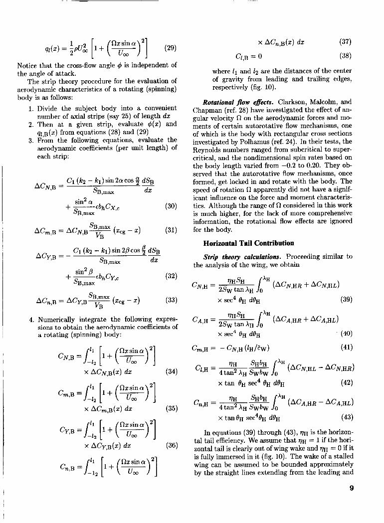
x A c n , B ( x ) d x (37)
C1,B = 0 (38)
where Z1 and Z2 are the distances of the center of gravity from leading and trailing edges, respectively (fig. 10).
Notice that the cross-flow angle 4 is independent of the angle of attack.
The strip theory procedure for the evaluation of aerodynamic characteristics of a rotating (spinning) body is as follows:
1. Divide the subject body into a convenient number of axial strips (say 25) of length d x
2. Then at a given strip, evaluate 4 ( x ) and q1 B(X) from equations (28) and (29)
3. Fiom the following equations, evaluate the aerodynamic coefficients (per unit length) of each strip:
C 1 (kq - kl) sin 2 0 cos Q dSB A ~ N , B = SB,max dx
+- EbhCX,c sin2 a
SB,max
sin2 p SB,max
+- cbhCY,c
(33)
4. Numerically integrate the following expres- sions to obtain the aerodynamic coefficients of a rotating (spinning) body:
R x sin a CN,B =rl -12 [ I+ ( urn )'I
x A ~ N , B ( x ) d~ (34)
C m , B = r l ['+ ( R x urn sin a )'] -12
R x sin a c n , B = r l - 12 ['+ ( u,
Rotational Jlow effects. Clarkson, Malcolm, and Chapman (ref. 28) have investigated the effect of an- gular velocity R on the aerodynamic forces and mo- ments of certain autorotative flow mechanisms, one of which is the body with rectangular cross sections investigated by Polhamus (ref. 24). In their tests, the Reynolds numbers ranged from subcritical to super- critical, and the nondimensional spin rates based on the body length varied from -0.2 to 0.20. They ob- served that the autorotative flow mechanisms, once formed, get locked in and rotate with the body. The speed of rotation R apparently did not have a signif- icant influence on the force and moment characteris- tics. Although the range of R considered in this work is much higher, for the lack of more comprehensive information, the rotational flow effects are ignored for the body.
Horizontal Tail Contribution
Strip theoty calculations. Proceeding similar to the analysis of the wing, we obtain
x tanOH sec4~H dflH (43)
In equations (39) through (43), q~ is the horizon- tal tail efficiency. We assume that QH = 1 if the hori- zontal tail is clearly out of wing wake and VH = 0 if it is fully immersed in it (fig. 10). The wake of a stalled wing can be assumed to be bounded approximately by the straight lines extending from the leading and
9
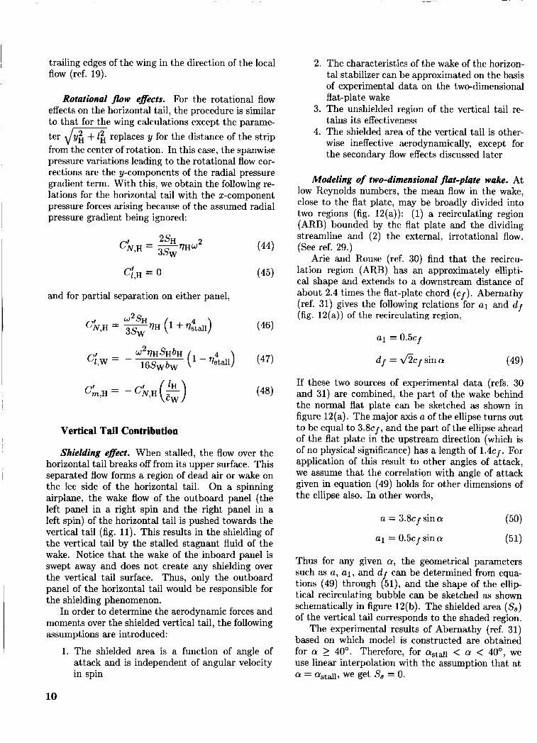
trailing edges of the wing in the direction of the local flow (ref. 19).
Rotational flow effects. For the rotational flow effects on the horizontal tail, the procedure is similar to that for the wing calculations except the parame- ter d m replaces y for the distance of the strip from the center of rotation. In this case, the spanwise pressure variations leading to the rotational flow cor- rections are the y-components of the radial pressure gradient term. With this, we obtain the following re- lations for the horizontal tail with the z-component pressure forces arising because of the assumed radial pressure gradient being ignored:
and for partial separation on either panel,
(44)
(45)
Vertical Tail Contribution
Shielding effect. When stalled, the flow over the horizontal tail breaks off from its upper surface. This separated flow forms a region of dead air or wake on the lee side of the horizontal tail. On a spinning airplane, the wake flow of the outboard panel (the left panel in a right spin and the right panel in a left spin) of the horizontal tail is pushed towards the vertical tail (fig. 11). This results in the shielding of the vertical tail by the stalled stagnant fluid of the wake. Notice that the wake of the inboard panel is swept away and does not create any shielding over the vertical tail surface. Thus, only the outboard panel of the horizontal tail would be responsible for the shielding phenomenon.
In order to determine the aerodynamic forces and moments over the shielded vertical tail, the following assumptions are introduced:
1. The shielded area is a function of angle of attack and is independent of angular velocity in spin
2. The characteristics of the wake of the horizon- tal stabilizer can be approximated on the basis of experimental data on the two-dimensional flat-plate wake
3. The unshielded region of the vertical tail re- tains its effectiveness
4. The shielded area of the vertical tail is other- wise ineffective aerodynamically, except for the secondary flow effects discussed later
Modeling of two-dimensional flat-plate wake. At low Reynolds numbers, the mean flow in the wake, close to the flat plate, may be broadly divided into two regions (fig. 12(a)): (1) a recirculating region (ARB) bounded by the flat plate and the dividing streamline and (2) the external, irrotational flow. (See ref. 29.)
Arie and Rouse (ref. 30) find that the recircu- lation region (ARB) has an approximately ellipti- cal shape and extends to a downstream distance of about 2.4 times the flat-plate chord (cf). Abernathy (ref. 31) gives the following relations for a1 and df (fig. 12(a)) of the recirculating region,
a1 = 0.5cj
df = h c f sin a
If these two sources of experimental data (refs. 30 and 31) are combined, the part of the wake behind the normal flat plate can be sketched as shown in figure 12(a). The major axis a of the ellipse turns out to be equal to 3.8cf, and the part of the ellipse ahead of the flat plate in the upstream direction (which is of no physical significance) has a length of 1.4cf. For application of this result to other angles of attack, we assume that the correlation with angle of attack given in equation (49) holds for other dimensions of the ellipse also. In other words,
(49)
a = 3.8cf sina (50)
a1 = 0.5cf sin a (51)
Thus for any given a, the geometrical parameters such as a, a l , and d can be determined from equa- tions (49) through hl), and the shape of the ellip tical recirculating bubble can be sketched as shown schematically in figure 12(b). The shielded area (S,) of the vertical tail corresponds to the shaded region.
The experimental results of Abernathy (ref. 31) based on which model is constructed are obtained for a 2 40'. Therefore, for astall < a < 40°, we use linear interpolation with the assumption that at a = astall, we get S, = 0.
10
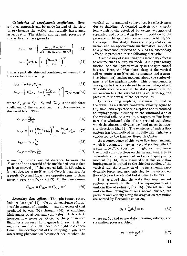
Calculation of aerodynamic coefficients. Here, a direct approach can be made instead of the strip theory because the vertical tail normally has a small aspect ratio. The sideslip and dynamic pressure at the vertical tail are given by
} (52) 2w (1VlbW) sin a
1 + [2w ( lV/bw) sin aI2 ov = -sin-’
Under a partially shielded condition, we assume that the side force is given by
where S V , ~ @ = SV - S, and C$,v is the side-force coefficient of the vertical tail. Its determination is discussed later. Then
FY,V CY,V = -
QSW
hV C1,V = CY,V -
bW
1V c,,v = -Cy,v- bW
(59)
where h v is the vertical distance between the X-axis and the centroid of the unshielded area (taken positive upwards) of the vertical tail. In left spin, w is negative, pV is positive, and Cy,, is negative. As a result, C1,V and Cn,v have opposite signs to those given in equations (58) and (59). Further, we assume
c N , V = Cm,V = c A , V = 0 (60)
Secondary frow effects. The spin-tunnel rotary balance data (ref. 11) indicate the existence of a no- ticeable amount of damping in yaw (in excess of that predicted by eqs. (52) through (54)) at combined high angles of attack and spin rates. Such a fact, however, may never be noticed by the pilot in spin flight tests because the magnitude of such a damp ing effect may be small under spin flight test condi- tions. This development of the damping in yaw is an interesting phenomenon because it occurs when the
vertical tail is assumed to have lost its effectiveness due to shielding. A detailed analysis of this prob- lem which is characterized by extensive regions of separated and recirculating flows, in addition to the presence of the spin rate, is considered to be beyond the scope of this study. However, a physical expla- nation and an approximate mathematical model of this phenomenon, referred to here as the “secondary effect,” is presented in the following discussion.
A simple way of visualizing this secondary effect is to assume that the airplane model is in a pure rotary motion, and the upward velocity in the spin tunnel is zero. Here, the “flat-plate” drag of the vertical tail generates a positive rolling moment and a nega- tive (damping) yawing moment about. the center-of- gravity of the airplane model. This phenomenon is analogous to the one referred to as secondary effect. The difference here is that the static pressure in the air surrounding the vertical tail is equal to p,, the pressure in the wake of the horizontal tail.
On a spinning airplane, the mass of fluid in the wake has a relative transverse velocity equal to RZv sin a with respect to the airplane and is assumed to impinge perpendicularly on the windward side of the vertical tail. As a result, a stagnation line forms over the windward side of the vertical tail about which the airstream divides itself and moves in oppo- site directions (fig. 13). The existence of such a flow pattern has been noticed in the full-scale flight tests conducted by the Langley Research Center.
As a consequence of this wake flow impingement, which is designated here as “secondary flow effect,” a side force Fy,v (positive in right spin and nega- tive in left spin) develops on the fin and generates an autorotative rolling moment and an antispin yawing moment (fig. 14). It is assumed that this wake flow impingement is limited to the shielded portion of the vertical tail. An estimation of the incremental aero- dynamic forces and moments due to the secondary flow effect on the vertical tail is done as follows.
It is assumed that the wake flow impingement pattern is similar to that of the impingement of a uniform flow of radius rj (fig. 15). (See ref. 32). For uniform flow impingement on a normal surface, the pressure and velocity along the stagnation streamline are related by Bernouli’s equation,
where p, , Us, and po are static pressure, velocity, and stagnation pressure. Also,
11
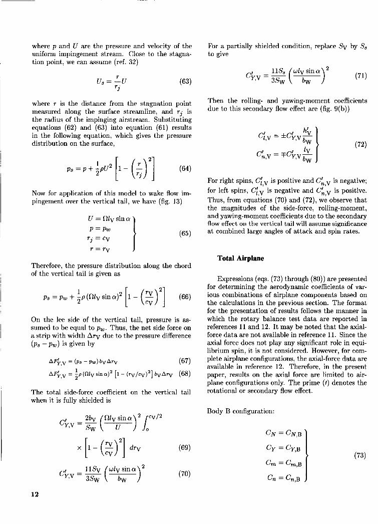
where p and U are the pressure and velocity of the uniform impingement stream. Close to the stagna- tion point, we can assume (ref. 32)
where r is the distance from the stagnation point measured along the surface streamline, and r j is the radius of the impinging airstream. Substituting equations (62) and (63) into equation (61) results in the following equation, which gives the pressure distribution on the surface,
Now for application of this model to wake flow im- pingement over the vertical tail, we have (fig. 13)
I U = Rlv sin a P = Pw
T j = cv
Therefore, the pressure distribution along the chord of the vertical tail is given as
1 2
p , = p , + -p(fIlVsina)
On the lee side of the vertical tail, pressure is as- sumed to be equal to p,. Thus, the net side force on a strip with width Ar, due to the pressure difference ( p , - pw) is given by
The total side-force coefficient on the vertical tail when it is fully shielded is
x [I- (x)'] dv
For a partially shielded condition, replace Sv by S, to give
2
(71) llS, wlv sina
c'9v=K ( bw ) Then the rolling- and yawing-moment coefficients due to this secondary flow effect are (fig. 9(b))
For right spins, Ci,v is positive and CL,v is negative; for left spins, Ci,v is negative and is positive. Thus, from equations (70) and (72), we observe that the magnitudes of the side-force, rolling-moment, and yawing-moment coefficients due to the secondary flow effect on the vertical tail will assume significance at combined large angles of attack and spin rates.
Total Airplane
Expressions (eqs. (73) through (80)) are presented for determining the aerodynamic coefficients of var- ious combinations of airplane components based on the calculations in the previous section. The format for the presentation of results follows the manner in which the rotary balance test data are reported in references 11 and 12. It may be noted that the axial- force data are not available in reference 11. Since the axial force does not play any significant role in equi- librium spin, it is not considered. However, for com- plete airplane configurations, the axial-force data are available in reference 12. Therefore, in the present paper, results on the axial force are limited to air- plane configurations only. The prime ( I ) denotes the rotational or secondary flow effect.
(73)
12
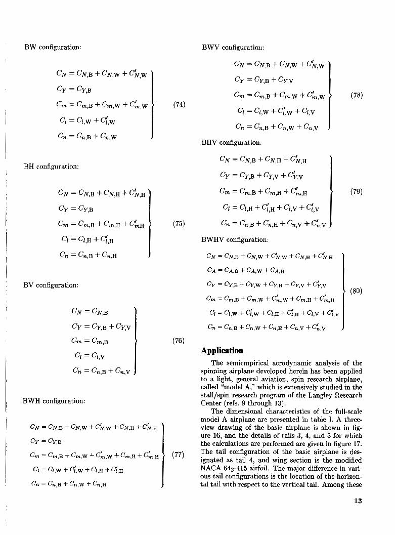
BW configuration: BWV configuration:
BH configuration:
(75)
BV configuration:
BWH configuration:
BHV configuration:
BWHV configuration:
Application The semiempirical aerodynamic analysis of the
spinning airplane developed herein has been applied to a light, general aviation, spin research airplane, called “model A,” which is extensively studied in the stall/spin research program of the Langley Research Center (refs. 9 through 13).
The dimensional characteristics of the full-scale model A airplane are presented in table I. A three- view drawing of the basic airplane is shown in fig- ure 16, and the details of tails 3, 4, and 5 for which the calculations are performed are given in figure 17. The tail configuration of the basic airplane is des- ignated as tail 4, and wing section is the modified NACA 642-415 airfoil. The major difference in vari- ous tail configurations is the location of the horizon- tal tail with respect to the vertical tail. Among these
13
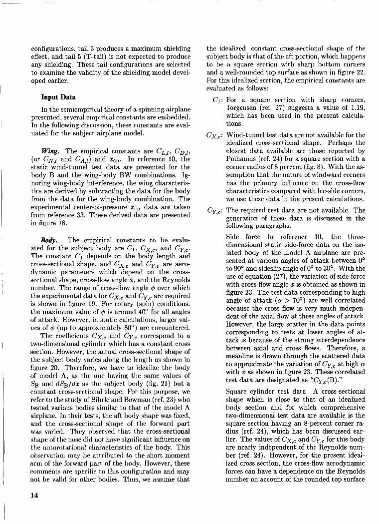
configurations, tail 3 produces a maximum shielding effect, and tail 5 (T-tail) is not expected to produce any shielding. These tail configurations are selected to examine the validity of the shielding model devel- oped earlier.
Input Data In the semiempirical theory of a spinning airplane
presented, several empirical constants are embedded. In the following discussion, these constants are eval- uated for the subject airplane model.
Wing. The empirical constants are C L , ~ , C O , ~ , (or C N , ~ and C A , ~ ) and Zcp. In reference 10, the static wind-tunnel test data are presented for the body B and the wing-body BW combinations. Ig- noring wing-body interference, the wing characteris- tics are derived by subtracting the data for the body from the data for the wing-body combination. The experimental center-of-pressure Zcp data are taken from reference 33. These derived data are presented in figure 18.
Body. The empirical constants to be evalu- ated for the subject body are C1, CX,,, and Cy,,. The constant C1 depends on the body length and cross-sectional shape, and Cx,, and Cy,, are aero- dynamic parameters which depend on the cross- sectional shape, cross-flow angle 4, and the Reynolds number. The range of cross-flow angle 4 over which the experimental data for Cx,, and Cy,, are required is shown in figure 19. For rotary (spin) conditions, the maximum value of 4 is around 40" for all angles of attack. However, in static calculations, larger val- ues of 4 (up to approximately 80") are encountered.
The coefficients Cx,, and Cy,, correspond to a two-dimensional cylinder which has a constant cross section. However, the actual cross-sectional shape of the subject body varies along the length as shown in figure 20. Therefore, we have to idealize the body of model A, as the one having the same values of SB and d S B / d x as the subject body (fig. 21) but a constant cross-sectional shape. For this purpose, we refer to the study of Bihrle and Bowman (ref. 23) who tested various bodies similar to that of the model A airplane. In their tests, the aft body shape was fixed, and the cross-sectional shape of the forward part was varied. They observed that the cross-sectional shape of the nose did not have significant influence on the autorotational characteristics of t,he body. This observation may be attributed to the short moment arm of the forward part of the body. However, these comments are specific to this configuration and may not be valid for other bodies. Thus, we assume that
the idealized constant cross-sectional shape of the subject body is that of the aft portion, which happens to be a square section with sharp bottom corners and a well-rounded top surface as shown in figure 22. For this idealized section, the empirical constants are evaluated as follows:
C1: For a square section with sharp corners, Jorgensen (ref. 27) suggests a value of 1.19, which has been used in the present calcula- tions.
Cx,,: Wind-tunnel test data are not available for the idealized cross-sectional shape. Perhaps the closest data available are those reported by Polhamus (ref. 24) for a square section with a corner radius of 8 percent (fig. 8). With the as- sumption that the nature of windward corners has the primary influence on the cross-flow characteristics compared with lee-side corners, we use these data in the present calculations.
Cy,,: The required test data are not available. The generation of these data is discussed in the following paragraphs:
Side force-In reference 10, the three- dimensional static side-force data on the iso- lated body of the model A airplane are pre- sented at various angles of attack between 0' to 90" and sideslip angle of 0" to 30". With the use of equation (27), the variation of side force with cross-flow angle 4 is obtained as shown in figure 23. The test data corresponding to high angle of attack (a > 70') are well correlated because the cross flow is very much indepen- dent of the axial flow at these angles of attack. However, the large scatter in the data points corresponding to tests at lower angles of at- tack is because of the strong interdependence between axial and cross flows. Therefore, a meanline is drawn through the scattered data to approximate the variation of Cy,, at high a with 4 as shown in figure 23. These correlated test data are designated as "Cy,,(B)."
Square cylinder test data-A cross-sectional shape which is close to that of an idealized body section and for which comprehensive two-dimensional test data are available is the square section having an &percent corner ra- dius (ref. 24), which has been discussed ear- lier. The values of Cx,, and Cy,, for this body are nearly independent of the Reynolds num- ber (ref. 24). However, for the present ideal- ized cross section, the cross-flow aerodynamic forces can have a dependence on the Reynolds number on account of the rounded top surface
14
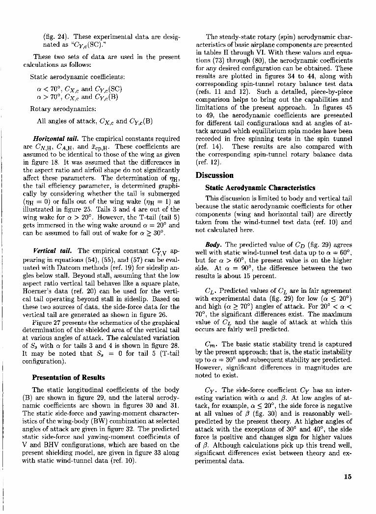
(fig. 24). These experimental data are desig- nated as "Cy,,(SC)."
These two sets of data are used in the present calculations as follows:
Static aerodynamic coefficients:
a < 70°, Cx,, and Cy,,(SC) a > 70', C X , ~ and Cy,,(B)
Rotary aerodynamics:
All angles of attack, Cx,, and Cy,,(B)
Horizontal tail. The empirical constants required are CN,H, CA,H, and Z C p , ~ . These coefficients are assumed to be identical to those of the wing as given in figure 18. It was assumed that the differences in the aspect ratio and airfoil shape do not significantly affect these parameters. The determination of VH, the tail efficiency parameter, is determined graphi- cally by considering whether the tail is submerged ( q ~ = 0) or falls out of the wing wake (VH = 1) as illustrated in figure 25. Tails 3 and 4 are out of the wing wake for Q > 20'. However, the T-tail (tail 5) gets immersed in the wing wake around a = 20' and can be assumed to fall out of wake for a 2 30'.
Vertical tail. The empirical constant C;,v ap- pearing in equations (54), (55), and (57) can be eval- uated with Datcom methods (ref. 19) for sideslip an- gles below stall. Beyond stall, assuming that the low aspect ratio vertical tail behaves like a square plate, Hoerner's data (ref. 20) can be used for the verti- cal tail operating beyond stall in sideslip. Based on these two sources of data, the side-force data for the vertical tail are generated as shown in figure 26.
Figure 27 presents the schematics of the graphical determination of the shielded area of the vertical tail at various angles of attack. The calculated variation of S, with a for tails 3 and 4 is shown in figure 28. It may be noted that S, = 0 for tail 5 (T-tail configuration).
Presentation of Results
The static longitudinal coefficients of the body (B) are shown in figure 29, and the lateral aerody- namic coefficients are shown in figures 30 and 31. The static side-force and yawing-moment character- istics of the wing-body (BW) combination at selected angles of attack are given in figure 32. The predicted static side-force and yawing-moment coefficients of V and BHV configurations, which are based on the present shielding model, are given in figure 33 along with static wind-tunnel data (ref. 10).
The steady-state rotary (spin) aerodynamic char- acteristics of basic airplane components are presented in tables I1 through VI. With these values and equa- tions (73) through (80), the aerodynamic coefficients for any desired configuration can be obtained. These results are plotted in figures 34 to 44, along with corresponding spin-tunnel rotary balance test data (refs. 11 and 12). Such a detailed, piece-by-piece comparison helps to bring out the capabilities and limitations of the present approach. In figures 45 to 49, the aerodynamic coefficients are presented for different tail configurations and at angles of at- tack around which equilibrium spin modes have been recorded in free spinning tests in the spin tunnel (ref. 14). These results are also compared with the corresponding spin-tunnel rotary balance data (ref. 12).
Discussion Static Aerodynamic Characteristics This discussion is limited to body and vertical tail
because the static aerodynamic coefficients for other components (wing and horizontal tail) are directly taken from the wind-tunnel test data (ref. 10) and not calculated here.
Body. The predicted value of CD (fig. 29) agrees well with static wind-tunnel test data up to a = 60°, but for a > 60°, the present value is on the higher side. At a = 90°, the difference between the two results is about 15 percent.
C,. Predicted values of CL are in fair agreement with experimental data (fig. 29) for low (a 5 20') and high (a 2 70') angles of attack. For 20' < a < 70°, the significant differences exist. The maximum value of C, and the angle of attack at which this occurs are fairly well predicted.
C,. The basic static stability trend is captured by the present approach; that is, the static instability up to Q = 30' and subsequent stability are predicted. However, significant differences in magnitudes are noted to exist.
Cy. The side-force coefficient Cy has an inter- esting variation with a and p. At low angles of at- tack, for example, a 5 20', the side force is negative at all values of /3 (fig. 30) and is reasonably well- predicted by the present theory. At higher angles of attack with the exceptions of 30' and 40°, the side force is positive and changes sign for higher values of p. Although calculations pick up this trend well, significant differences exist between theory and ex- perimental data.
15
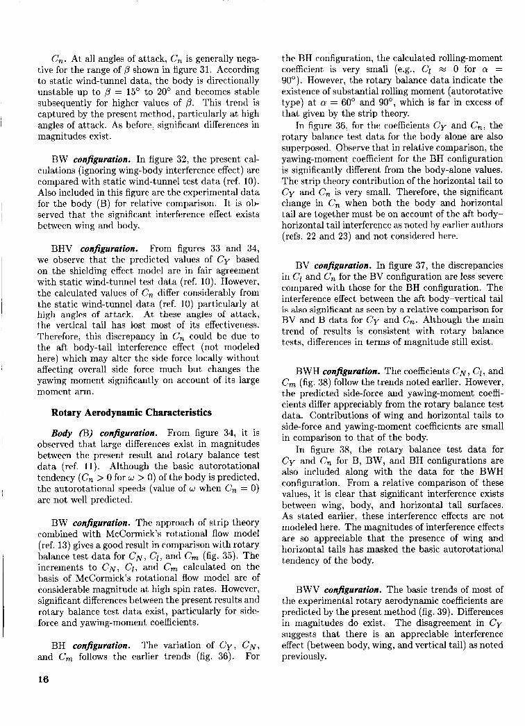
Cn. At all angles of attack, Cn is generally nega- tive for the range of p shown in figure 31. According to static wind-tunnel data, the body is directionally unstable up to p = 15' to 20' and becomes stable subsequently for higher values of p. This trend is captured by the present method, particularly at high angles of attack. As before, significant differences in magnitudes exist.
BW configuration. In figure 32, the present cal- culations (ignoring wing-body interference effect) are compared with static wind-tunnel test data (ref. 10). Also included in this figure are the experimental data for the body (B) for relative comparison. It is ob- served that the significant interference effect exists between wing and body.
BHV configuration. From figures 33 and 34, we observe that the predicted values of Cy based on the shielding effect model are in fair agreement with static wind-tunnel test data (ref. 10). However, the calculated values of Cn differ considerably from the static wind-tunnel data (ref. 10) particularly at high angles of attack. At these angles of attack, the vertical tail has lost most of its effectiveness. Therefore, this discrepancy in Cn could be due to the aft body-tail interference effect (not modeled here) which may alter the side force locally without affecting overall side force much but changes the yawing moment significantly on account of its large moment arm.
Rotary Aerodynamic Characteristics
Body (B) configuration. From figure 34, it is observed that large differences exist in magnitudes between the present result and rotary balance test data (ref. 11). Although the basic autorotational tendency (Cn > 0 for w > 0) of the body is predicted, the autorotational speeds (value of w when Cn = 0) are not well predicted.
BW configuration. The approach of strip theory combined with McCormick's rotational flow model (ref. 13) gives a good result in comparison with rotary balance test data for C N , Ci, and Cm (fig. 35). The increments to C N , Cl, and Cm calculated on the basis of McCormick's rotational flow model are of considerable magnitude at high spin rates. However, significant differences between the present results and rotary balance test data exist, particularly for side- force and yawing-moment coefficients.
BH configuration. The variation of C y , C N , For and Cm follows the earlier trends (fig. 36).
the BH configuration, the calculated rolling-moment coefficient is very small (e.g., Cl x 0 for a = 90'). However, the rotary balance data indicate the existence of substantial rolling moment (autorotative type) at a = 60' and 90°, which is far in excess of that given by the strip theory.
In figure 36, for the coefficients Cy and Cn, the rotary balance test data for the body alone are also superposed. Observe that in relative comparison, the yawing-moment coefficient for the BH configuration is significantly different from the body-alone values. The strip theory contribution of the horizontal tail to C y and C, is very small. Therefore, the significant change in Cn when both the body and horizontal tail are together must be on account of the aft body- horizontal tail interference as noted by earlier authors (refs. 22 and 23) and not considered here.
BV configuration. In figure 37, the discrepancies in Cl and Cn for the BV configuration are less severe compared with those for the BH configuration. The interference effect between the aft body-vertical tail is also significant as seen by a relative comparison for BV and B data for Cy and Cn. Although the main trend of results is consistent with rotary balance tests, differences in terms of magnitude still exist.
BWH configuration. The coefficients C N , Cl, and Cm (fig. 38) follow the trends noted earlier. However, the predicted side-force and yawing-moment coeffi- cients differ appreciably from the rotary balance test data. Contributions of wing and horizontal tails to side-force and yawing-moment coefficients are small in comparison to that of the body.
In figure 38, the rotary balance test data for Cy and Cn for B, BW, and BH configurations are also included along with the data for the BWH configuration. From a relative comparison of these values, it is clear that significant interference exists between wing, body, and horizontal tail surfaces. As stated earlier, these interference effects are not modeled here. The magnitudes of interference effects are so appreciable that the presence of wing and horizontal tails has masked the basic autorotational tendency of the body.
BWV configuration. The basic trends of most of the experimental rotary aerodynamic coefficients are predicted by the present method (fig. 39). Differences in magnitudes do exist. The disagreement in Cy suggests that there is an appreciable interference effect (between body, wing, and vertical tail) as noted previously.
16
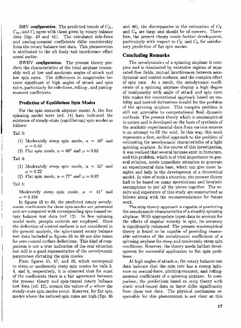
BHV configuration. The predicted trends of C N , Cm, and Cl agree with those given by rotary balance data (figs. 40 and 41). The calculated side-force and yawing-moment coefficients differ considerably from the rotary balance test data. This phenomenon is attributed to the aft body-tail interference effect noted earlier.
BWHV configuration. The present theory pre- dicts the characteristics of the total airplane reason- ably well at low and moderate angles of attack and low spin rates. The differences in magnitudes be- come significant at high angles of attack and spin rates, particularly for side-force, rolling-, and yawing- moment coefficients.
Prediction of Equilibrium Spin Modes
For the spin research airplane model A, the free spinning model tests (ref. 14) have indicated the existence of steady-state (equilibrium) spin modes as follows:
Tail 3:
(1) Moderately steep spin mode, a = 50' and
(2) Flat spin mode, a = 80' and w = 0.62 w = 0.33
Tail 4:
(1) Moderately steep spin mode, a = 35' and
(2) Flat spin mode, a = 77' and w = 0.92 w = 0.22
Tail 5:
Moderately steep spin mode, a = 41' and w = 0.234 In figures 45 to 49, the predicted rotary aerody-
namic coefficients for these spin modes are presented and are compared with corresponding spin-tunnel ro- tary balance test data (ref. 12). In free spinning model tests, prospin controls are employed. Since the deflection of control surfaces is not considered in the present analysis, the spin-tunnel rotary balance test data included in figures 35 to 39 are also taken for zero control surface deflections. This kind of com- parison is not a true indication of the real situation but still is a good representative of the aerodynamic parameters dictating the spin modes.
From figures 45, 47, and 49, which correspond to steep or moderately steep spin modes for tails 3, 4, and 5, respectively, it is observed that for most of the coefficients there is a fair agreement between the present theory and spin-tunnel rotary balance test data (ref. 12), around the values of w where the steady-state spin modes occur. However, for flat spin modes where the reduced spin rates are high (figs. 46
and 48), the discrepancies in the estimation of Cy and Cn are large and should be of concern. There- fore, the present theory needs further development, particularly with respect to Cy and Cn for satisfac- tory prediction of flat spin modes.
Concluding Remarks The aerodynamics of a spinning airplane is com-
plex and is dominated by extensive regions of sepa- rated flow fields, mutual interferences between aero- dynamic and control surfaces, and the complex effect of spin rate. As a result, the aerodynamic coeffi- cients of a spinning airplane display a high degree of nonlinearity with angle of attack and spin rate; this makes the conventional approach based on sta- bility and control derivatives invalid for the problem of the spinning airplane. This complex problem is still not amenable to computational fluid dynamic methods. The present theory which is semiempirical in nature and is developed on the basis of synthesis of the available experimental data from various sources is an attempt to fill the void. In this way, this work represents a first, unified approach to the problem of estimating the aerodynamic characteristics of a light spinning airplane. In the course of this investigation, it was realized that several lacunae exist in literature, and this problem, which is of vital importance to gen- eral aviation, needs immediate attention to generate an experimental data base, which can give more in- sights and help in the development of a theoretical model. In view of such a situation, the present theory had to be based on many speculations and heuristic assumptions to put all the pieces together. The re- sults and experience of this study are summarized as follows along with the recommendations for future work.
The strip theory approach is capable of predicting the aerodynamic characteristics of a steadily spinning airplane. With appropriate input data to account for the effects of angular velocity in spin, its accuracy is significantly enhanced. The present semiempirical theory is found to be capable of providing reason- able estimates of the aerodynamic coefficients of a spinning airplane for steep and moderately steep spin conditions. However, the theory needs further devel- opment for successful application to flat spin prob- lems.
At high angles of attack a, the rotary balance test data indicate that the spin rate has a strong influ- ence on normal-force, pitching-moment, and rolling- moment coefficients of a spinning airplane. In com- parison, the predictions based on strip theory with static wind-tunnel data as input differ significantly from these test data. The physical mechanism re- sponsible for this phenomenon is not clear at this
17
stage as there is no experimental data base which records flow pattern or pressure distributions over a spinning wing and throws some light on the physics of the flow.
No validated aerodynamic models for stalled spin- ning wings exist. McCormick (NASA CR-165680) hypothesizes incremental changes in the aerodynamic forces and moments caused by the spanwise pressure gradient on the lee side of the wing due to centrifu- gal force. Although the inclusion of the increments improves the comparison of strip theory with exper- imental test data, there is a dearth of evidence nec- essary to validate the underlying assumptions. Lo- cal flow measurements of stalled spinning wings are needed to enable the formulation of a comprehensive theory.
A semiempirical method is developed for the pre- diction of body aerodynamic characteristics at high angles of attack and sideslip. This approach gives the required static input data in the strip theory for the spinning airplane.
All the mutua l interference effects between vari- ous components are not considered except the shield- ing of vertical tail surface by the wake of horizontal tail. A simple procedure for estimating the shielded area of the vertical tail is presented. Increments to aerodynamic coefficients on account of the secondary flow within the shielded part of the vertical tail are estimated by a simple analysis of wake flow impinge- ment on the vertical tail.
Some of the mutual interference effects between body, wing, and tail surfaces of a spinning airplane, which are not considered herein, are found to be large and significant. Of particular concern is the interfer- ence effect between aft body and horizontal tail sur- faces, which can have a strong influence on side force and yawing moments. Further studies are necessary in this direction to gain a better understanding of these complex effects.
It is recommended that further research be initi- ated to study the aerodynamics of the spinning air- plane at high angles of attack and spin rate. Flow visualization and pressure distribution measurements should be carried out along with direct force and moment coefficients so as to increase the process of understanding and development of a comprehensive theory for a spinning light airplane.
NASA Langley Research Center Hampton, VA 23665-5225 November 5, 1987
18
References 1.
2.
3.
4.
5.
6.
7.
8.
9.
Silver, Brent W.: Statistical Analysis of General Avi- ation Stall Spin Accidents. [Preprint] 760480, SOC. of Automotive Engineers, Apr. 1976. Dickinson, B.: Aircraft Stability and Control for Pilots and Engineers. Sir Isaac Pitman & Sons Ltd., c.1968. Glauert, H.: The Investigation of the Spin of an Aero- plane. R. & M. No. 618, British Advisory Committee for Aeronautics, June 1919. Gates, S. B.; and Bryant, L. W.: The Spinning of Aeroplanes. R. & M. No. 1001, British Aeronautical Research Council, 1927. Wykes, John H.; Casteel, Gilbert R.; and Collins, Richard A.: An Analytical Study of the Dynamics of Spin- ning Aircraft. Part I-Flight Test Data Analyses and Spin Calculations. WADC Tech. Rep. 58-381, Pt. I, U.S. Air Force, Dec. 1958. (Available from DTIC as AD 203 788.) Bamber, M. J.; and House, R. 0.: Spinning Characteris- tics of the XN2Y-1 Airplane Obtained From the Spinning Balance and Compared With Results From the Spinning Tunnel and From Flight Tests. NACA Rep. 607, 1937. Bihrle, William, Jr.; and Barnhart, Billy: Spin Pre- diction Techniques. A Collection of Technical Papers- AIAA Atmospheric Flight Mechanics Conference, Aug. 1980, pp. 76-82. (Available as AIAA-80-1564.) Tischler, M. B.; and Barlow, J. B.: Determination of the Spin and Recovery Characteristics of a General Aviation Design. J . Aircr., vol. 18, no. 4, Apr. 1981, pp. 238-244. Himmelskamp, H.: Profile Investigations on a Rotating Airscrew. Rep. & Transl. No. 832, British Ministry of Aircraft Products Volkenrode, Sept. 1, 1947.
10. Bihrle, William, Jr.; Barnhart, Billy; and Pantason, Paul: Static Aerodynamic Characteristics of a Typical Single-Engine Low- Wing General Aviation Design for an Angle-of-Attack Range of -8' to 90". NASA CR-2971, 1978.
11. Bihrle, William, Jr.; Hultberg, Randy S.; and Mulcay, William: Rotary Balance Data for a Typical Single-Engine Low- Wing General Aviation Design for an Angle-of-Attack Range of 30" to 90". NASA CR-2972, 1978.
12. Hultberg, Randy S.; and Mulcay, William: Rotary Bal- ance Data for a Typical Single-Engine General Aviation Design for an Angle-of-Attack Range of g to 90". I- Low- Wing Model A . NASA CR-3100, 1980.
13. McCormick, Barnes W.: The Prediction of Normal Force and Rolling Moment Coeficients for a Spinning Wing. NASA CR-165680, 1981.
14. Burk, Sanger M., Jr.; Bowman, James S., Jr.; and White, William L.: Spin- Tunnel Investigation of the Spinning Characteristics of Typical Single-Engine Gen- eral Aviation Airplane Designs. I-Low- Wing Model A: Effects of Tail Configurations. NASA TP-1009, 1977.
15. Staff, Langley Research Center: Exploratory Study of the Effects of Wing-Leading-Edge Modifications on the Stall/Spzn Behavior of a Light General Aviation Airplane.
16. Pamadi, Bandu N.; and Taylor, Lawrence W., Jr.: An Estimation of Aerodynamic Forces and Moments on an
NASA TP-1589, 1979.
Airplane Model Under Steady State Spin Conditions.
17. Pamadi, Bandu N.; and Taylor, Lawrence W., Jr.: An Evaluation of Aerodynamics Modeling of Spinning Light Airplanes. AIAA-83-0368, Jan. 1983.
18. Poppen, William A., Jr.: A Method for Estimating the Rolling Moment Due to Spin Rate for Arbitrary Planform Wings. NASA TM-86365, 1985.
19. USAF Stability and Control Datcom. Contracts AF33(616)-6460 and F33615-764-3061, McDonnell Douglas Corp., Oct. 1960. (Revis. Apr. 1978.)
20. Hoerner, Sighard F.: Fluid-Dynamic Drag. Hoerner Fluid Dynamics (Brick Town, N.J.), c.1965.
21. Critzos, Chris C.: Heyson, Harry H.; and Boswinkle, Robert W., Jr.: Aerodynamic Characteristics of NACA 001.2 Airfoil Section at Angles of Attack From 0" to 180". NACA TN 3361, 1955.
22. Beaurain, L. (Leo Kanner Associates, transl.): General Study oJLight Plane Spin, Aft Fuselage Geometry, Part 1.
23. Bihrle, William, Jr.; and Bowman, James S., Jr.: Influ- ence of Wing, Fuselage, and Tail Design on Rotational Flow Aerodynamics Beyond Maximum Lift. J. Aircr., vol. 18, no. 11, Nov. 1981, pp. 920-925.
Effect of Flow Incidence and Reynolds Number on Low-Speed Aerodynamic Character- istics of Several Noncircular Cylinders With Applications to Directional Stability and Spinning. NASA TR R-29, 1959. (Supersedes NACA TN 4176.)
AIAA-82-1311, Aug. 1982.
NASA TT F-17,446, 1977.
24. Polhamus, Edward C.:
25. Allen, H. Julian: Estimation of the Forces and Moments Acting on Inclined Bodies of Revolution of High Fineness Ratio. NACA RM A9126, 1949.
26. Munk, Max M.: The Aerodynamic Forces on Airship Hulls. NACA Rep. 184, 1924.
27. Jorgensen, Leland Howard: Prediction of Static Aerody- namic Characteristics for Slender Bodies Alone and With Lifting Surfaces to Very High Angles of Attack. NASA
28. Clarkson, M. H.; Malcolm, G. N.; and Chapman, G. T.: Experimental Determination of Post-Stall Rotary Derivatives for Airplane-Like Configurations at Several Reynolds Numbers. AIAA Paper 75-171, Jan. 1975.
29. Maull, D. J.: Mechanisms of Two and Three- Dimensional Base Drag. Aerodynamic Drag Mechanisms of Bluff Bodies and Road Vehicles, Gin0 Sovran, Thomas Morel, and William T. Mason, Jr., eds., Plenum Press,
30. Arie, Mikio; and Rouse, Hunter: Experiments on Two- Dimensional Flow Over a Normal Wall. J. Fluid Mech., vol. 1, pt. 2, July 1956, pp. 129-141.
31. Abernathy, F. H.: Flow Over an Inclined Plate. J . Basic Eng., vol. 84, no. 3, Sept. 1962, pp. 380-388.
32. Schlichting, Hermann (J. Kestin, transl.): Boundary- Layer Theory, Sixth ed. McGraw-Hill Book Co., 1968.
33. Saini, Jugal Kishore: An Experimental Investigation of the Effects of Leading Edge Modifications on the Post- Stall Characteristics of an NACA 0015 Wing. M.S. Thesis, Univ. of Maryland, Aug. 1979.
TR R-474, 1977.
1978, pp. 137-159.
19
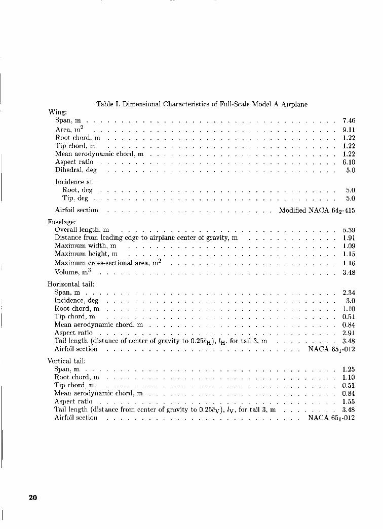
Table I . Dimensional Characteristics of Full-scale Model A Airplane Wing:
Span. m . . . . . . . . . . . . . . . . . . . . . . . . . . . . . . . . . . . . 7.46 Area. m2 . . . . . . . . . . . . . . . . . . . . . . . . . . . . . . . . . . . 9.11 Root chord. m . . . . . . . . . . . . . . . . . . . . . . . . . . . . . . . . . 1.22 Tip chord. m . . . . . . . . . . . . . . . . . . . . . . . . . . . . . . . . . 1.22 Mean aerodynamic chord. m . . . . . . . . . . . . . . . . . . . . . . . . . . . 1.22 Aspect ratio . . . . . . . . . . . . . . . . . . . . . . . . . . . . . . . . . . 6.10 Dihedral. deg . . . . . . . . . . . . . . . . . . . . . . . . . . . . . . . . . 5.0
Incidence at- Root. deg . . . . . . . . . . . . . . . . . . . . . . . . . . . . . . . . . . 5.0 Tip. deg . . . . . . . . . . . . . . . . . . . . . . . . . . . . . . . . . . . 5.0
Airfoil section . . . . . . . . . . . . . . . . . . . . . . . . Modified NACA 642-415
Overall length. m . . . . . . . . . . . . . . . . . . . . . . . . . . . . . . . 5.39 Distance from leading edge to airplane center of gravity. m . . . . . . . . . . . . . 1.91 Maximum width. m . . . . . . . . . . . . . . . . . . . . . . . . . . . . . . 1.09 Maximum height. m . . . . . . . . . . . . . . . . . . . . . . . . . . . . . . 1.15 Maximum cross-sectional area. m2 . . . . . . . . . . . . . . . . . . . . . . . . 1.16 Volume. m3 . . . . . . . . . . . . . . . . . . . . . . . . . . . . . . . . . . 3.48
Span. m . . . . . . . . . . . . . . . . . . . . . . . . . . . . . . . . . . . . 2.34 Incidence. deg . . . . . . . . . . . . . . . . . . . . . . . . . . . . . . . . . 3.0 Root chord. m . . . . . . . . . . . . . . . . . . . . . . . . . . . . . . . . . 1.10 Tip chord. m . . . . . . . . . . . . . . . . . . . . . . . . . . . . . . . . . 0.51 Mean aerodynamic chord. m . . . . . . . . . . . . . . . . . . . . . . . . . . . 0.84 Aspect ratio . . . . . . . . . . . . . . . . . . . . . . . . . . . . . . . . . . 2.91 Tail length (distance of center of gravity to 0.25C~) , 1 ~ . for tail 3. m . . . . . . . . . 3.48 Airfoil section . . . . . . . . . . . . . . . . . . . . . . . . . . . . NACA 651-012
Span. m . . . . . . . . . . . . . . . . . . . . . . . . . . . . . . . . . . . . 1.25 Root chord. m . . . . . . . . . . . . . . . . . . . . . . . . . . . . . . . . . 1.10 Tip chord. m . . . . . . . . . . . . . . . . . . . . . . . . . . . . . . . . . 0.51 Mean aerodynamic chord. m . . . . . . . . . . . . . . . . . . . . . . . . . . . 0.84 Aspect ratio . . . . . . . . . . . . . . . . . . . . . . . . . . . . . . . . . . 1.55
. . . . . . . . 3.48 Airfoil section . . . . . . . . . . . . . . . . . . . . . . . . . . . . NACA 651-012
Fuselage:
Horizontal tail:
Vertical tail:
Tail length (distance from center of gravity to 0.25Cv), lv. for tail 3. m
20
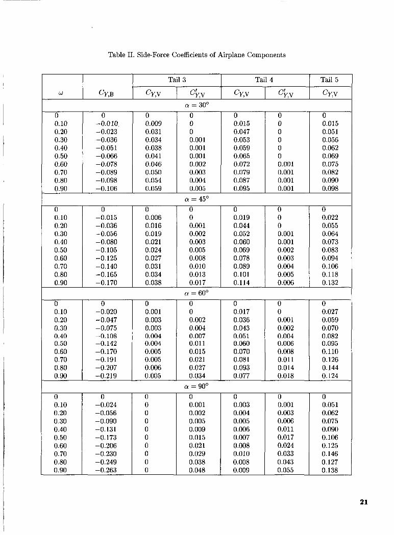
Table 11. Side-Force Coefficients of Airplane Components
Tail 3 Tail 4 I Tail 5 I I
0 0.019 0.044 0.052 0.060 0.069 0.078 0.089 0.101 0.114
0 0.10 0.20 0.30 0.40 0.50 0.60 0.70 0.80 0.90
0 0 0 0.001 0.001 0.002 0.003 0.004 0.005 0.006
0 0.10 0.20 0.30 0.40 0.50 0.60 0.70 0.80 0.90
0 0.10 0.20 0.30 0.40 0.50 0.60 0.70 0.80 0.90
0 -0.010, -0.023 -0.036 -0.051 -0.066 -0.078 -0.089 -0.098 -0.106
0 0 0 0 0 0 -0.020 0.001 0 0.017 0 0.027 -0.047 0.003 0.002 0.036 0.001 0.059 -0.075 0.003 0.004 0.043 0.002 0.070 -0.108 0.004 0.007 0.051 0.004 0.082 -0.142 0.004 0.01 1 0.060 0.006 0.095 -0.170 0.005 0.015 0.070 0.008 0.110 -0.191 0.005 0.021 0.081 0.011 0.126 -0.207 0.006 0.027 0.093 0.014 0.144 -0.219 0.005 0.034 0.077 0.018 0.124
0 -0.015 -0.036 -0.056 -0.080 -0.105 -0.125 -0.140 -0.165 -0.170
0 0.10 0.20 0.30 0.40 0.50 0.60 0.70 0.80 0.90
0 0.009 0.031 0.034 0.038 0.041 0.046 0.050 0.054 0.059
0 0 0 0 0 0 -0.024 0 0.001 0.003 0.001 0.051 -0.056 0 0.002 0.004 0.003 0.062 -0.090 0 0.005 0.005 0.006 0.075 -0.131 0 0.009 0.006 0.01 1 0.090 -0.173 0 0.015 0.007 0.017 0.106 -0.206 0 0.021 0.008 0.024 0.125 -0.230 0 0.029 0.010 0.033 0.146 -0.249 0 0.038 0.008 0.043 0.127 -0.263 0 0.048 0.009 0.055 0.138
0 0.006 0.016 0.019 0.021 0.024 0.027 0.031 0.034 0.038
CY = 30' 0 0 0 0.001 0.001 0.001 0.002 0.003 0.004 0.005
CY = 45' 0 0 0.001 0.002 0.003 0.005 0.008 0.010 0.013 0.017
CY = 60'
0 0.015 0.047 0.053 0.059 0.065 0.072 0.079 0.087 0.095
0 0 0 0 0 0 0.001 0.001 0.001 0.001
0 0.015 0.051 0.056 0.062 0.069 0.075 0.082 0.090 0.098
0 0.022 0.055 0.064 0.073 0.083 0.094 0.106 0.118 0.132
21
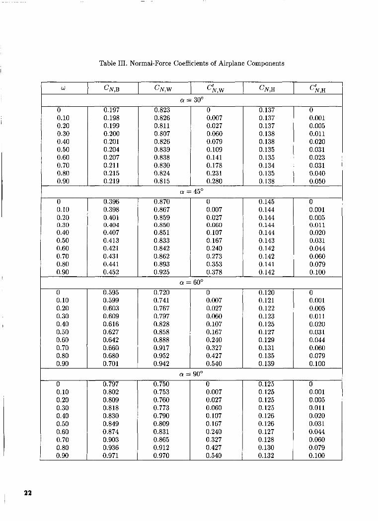
Table 111. Norma
0 0.197 0.823 0.10 0.198 0.826 0.20 0.199 0.811 0.30 0.200 0.807 0.40 0.201 0.826 0.50 0.204 0.839 0.60 0.207 0.838 0.70 0.211 0.830 0.80 0.215 0.824 0.90 0.219 0.815
Force Coefficients of Airplane Components
0 0.137 0 0.007 0.137 0.001 0.027 0.137 0.005 0.060 0.138 0.01 1 0.079 0.138 0.020 0.109 0.135 0.031 0.141 0.135 0.023 0.178 0.134 0.031 0.231 0.135 0.040 0.280 0.138 0.050
0 0.396 0.870 0.10 0.398 0.867 0.20 0.401 0.859 0.30 0.404 0.850 0.40 0.407 0.851 0.50 0.413 0.833 0.60 0.421 0.842 0.70 0.431 0.862 0.80 0.441 0.893 0.90 0.452 0.925
0 0.10 0.20 0.30 0.40 0.50 0.60 0.70 0.80 0.90
0 0.145 0 0.007 0.144 0.001 0.027 0.144 0.005 0.060 0.144 0.011 0.107 0.144 0.020 0.167 0.143 0.031 0.240 0.142 0.044 0.273 0.142 0.060 0.353 0.141 0.079 0.378 0.142 0.100
0 0.10 0.20 0.30 0.40 0.50 0.60 0.70 0.80 0.90
0 0.007 0.027 0.060 0.107 0.167 0.240 0.327 0.427 0.540
0.595 0.599 0.603 0.609 0.616 0.627 0.642 0.660 0.680 0.701
0.125 0 0.125 0.001 0.125 0.005 0.125 0.011 0.126 0.020 0.126 0.031 0.127 0.044 0.128 0.060 0.130 0.079 0.132 0.100
0.797 0.802 0.809 0.818 0.830 0.849 0.874 0.903 0.936 0.971
0.720 0.741 0.767 0.797 0.828 0.858 0.888 0.917 0.952 0.942
0 0.007 0.027 0.060 0.107 0.167 0.240 0.327 0.427 0.540
0.121 0.122 0.123 0.125 0.127 0.129 0.131 0.135 0.139
0 0.001 0.005 0.011 0.020 0.031 0.044 0.060 0.079 0.100
Q = goo 0.750 0.753 0.760 0.773 0.790 0.809 0.831 0.865 0.912 0.970
22
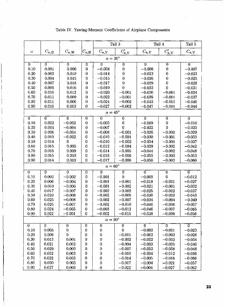
Table IV. Yawing-Moment Coefficients of Airplane Components
Tail 3 Tail 4 Tail 5
I Q = 30' 1 0 0.10 0.20 0.30 0.40 0.50 0.60 0.70 0.80 0.90
0 0 0 0.001 0.006 0 0.003 0.010 0 0.004 0.015 0 0.007 0.018 0 0.009 0.016 0 0.010 0.012 0 0.011 0.009 0 0.011 0.006 0 0.010 0.003 0
0 -0.004 -0.014 -0.015 -0.017 -0.019 -0.020 -0.022 -0.024 -0.027
0 0.10 0.20 0.30 0.40 0.50 0.60 0.70 0.80 0.90
-0.001 -0.001 -0.002 r -0.002
0 0 0 0 0 0 0 0 0.002 -0.002 0 -0.003 0 -0.009 0 -0.010 0.004 -0.004 0 -0.007 0 -0.022 0 -0.025 0.006 -0.004 0 -0.008 -0.001 -0.026 -0.001 -0.029 0.010 -0.002 0 -0.010 -0.001 -0.030 -0.001 -0.033 0.014 0 0 -0.010 -0.002 -0.034 -0.001 -0.037 0.015 0.005 0 -0.012 -0.004 -0.039 -0.002 -0.042 0.016 0.009 0 -0.014 -0.005 -0.044 -0.002 -0.048 0.015 0.010 0 -0.015 -0.006 -0.055 -0.003 -0.053 0.014 0.010 0 -0.017 -0.008 -0.056 -0.003 -0.060
-0.008 -0.023 -0.026 -0.029 -0.032 -0.036 -0.039 -0.043 ! -0.047
0 0 0 0 0.10 0.002 -0.002 0 0.20 0.006 -0.004 0 0.30 0.010 -0.006 0 0.40 0.017 -0.007 0 0.50 0.023 -0.008 0 0.60 0.025 -0.008 0 0.70 0.025 -0.007 0 0.80 0.024 -0.005 0 0.90 0.022 -0.001 0
0 0 0 0 0 0
-0.001 -0.001 -0.001 -0.001
0 0 0 0 0 -0.001 0 -0.009 0 -0.012 -0.001 -0.001 -0.018 -0.001 -0.027 -0.001 -0.002 -0.021 -0.001 -0.032 -0.002 -0.003 -0.025 -0.002 -0.037 -0.002 -0.005 -0.030 -0.003 -0.043 -0.002 -0.007 -0.034 -0.004 -0.049 -0.002 -0.010 -0.040 -0.006 -0.057 -0.003 -0.012 -0.046 -0.007 -0.065 -0.002 -0.015 -0.038 -0.009 -0.056
-0.007 -0.023 -0.025 -0.028 -0.031 -0.034 -0.037 -0.040 -0.044
0 0 0 0.10 0.003 0 0.20 0.008 0 0.30 0.013 0.001 0.40 0.021 0.002 0.50 0.029 0.003 0.60 0.032 0.003 0.70 0.032 0.003 0.80 0.030 0.003 0.90 0.027 0.003
0 0 0 0 0 0 0 0 0 -0.002 -0.001 -0.023 0 0 -0.001 -0.002 -0.002 -0.028 0 0 -0.002 -0.002 -0.003 -0.034 0 0 -0.004 -0.003 -0.005 -0.040 0 0 -0.007 -0.003 -0.008 -0.048 0 0 -0.010 -0.004 -0.012 -0.056 0 0 -0.014 -0.005 -0.016 -0.066 0 0 -0.017 -0.004 -0.021 -0.057 0 0 -0.022 -0.004 -0.027 -0.062
23
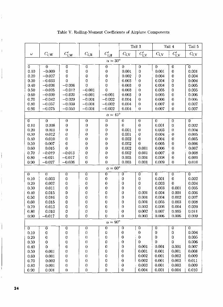
Table V. Rolling-Moment Coefficients of Airplane Components
Tail 3 Tail 4 1 Tail 5
0 0 0 0 0 0 0 0 0 0 0 0 0 0 0 0 0 0 0 0
0 0 0 0 0 0 0 0 0 0.001 0 0.001 0 0.002 0 0.002 0 0.003 0 0.004
CY = 30' 0 0.10 0.20 0.30 0.40 0.50 0.60 0.70 0.80 0.90
0 -0.009 -0.027 -0.033 -0.026 -0.025 -0.030 -0.042 -0.057 -0.075
0 0 0 0
-0.006 -0.012 -0.020 -0.029 -0.039 -0.050
0 0 0 0 0
-0.001 -0.001 -0.001 -0.001 -0.001
0 0.001 0.002 0.003 0.003 0.003 0.003 0.004 0.004 0.004
0 0.001 0.004 0.004 0.004 0.005 0.005 0.006 0.007 0.007
0 0.001 0.004 0.004 0.005 0.005 0.006 0.006 0.007 0.007
0 0 0 0 0 0
-0.001 -0.002 -0.002 -0.002
0 0 0 0 0 0 0 0 0 0
0 0 0 0 0 0 0 0 0 0
CY = 45' 0 0.008 0.011 0.012 0.010
-0.007 -0.015 -0.019 -0.021 -0.027
0 0 0 0 0 0 0
-0.013 -0.017 -0.036
0 0 0 0 0 0 0 0 0 0
0 0 0 0 0 0 0 0 0 0
0 0 0.001 0.001 0.002 0.002 0.002 0.002 0.003 0.003
0 0 0 0 0 0 0.001 0.001 0.001 0.001
0 0.001 0.003 0.004 0.004 0.005 0.006 0.007 0.008 0.009
0 0 0 0 0 0 0 0 0 0
0 0.10 0.20 0.30 0.40 0.50 0.60 0.70 0.80 0.90
0 0.002 0.004 0.005 0.005 0.006 0.007 0.008 0.009 0.010
CY = 60' 0 0.10 0.20 0.30 0.40 0.50 0.60 0.70 0.80 0.90
0 0.003 0.007 0.01 1 0.015 0.016 0.015 0.013 0.010
-0.017
0 0 0 0 0 0 0 0 0 0
0 0 0 0 0 0 0 0 0 0
0 0 0 0 0 0 0 0 0 0 ff = 90'
0 0 0 0 0 0 0 0 0 0
0 0 0 0 0.001 0.001 0.001 0.002 0.002 0.003
0 0.001 0.003 0.003 0.004 0.004 0.005 0.006 0.007 0.006
0 0 0 0.001 0.001 0.002 0.003 0.004 0.005 0.006
0 0.002 0.004 0.005 0.006 0.007 0.008 0.009 0.01 1 0.009
0 0.004 0.005 0.006 0.007 0.008 0.009 0.011 0.009 0.010
0 0 0 0 0.001 0.001 0.002 0.003 0.003 0.004
0 0 0 0 0.001 0.001 0.001 0.001 0.001 0.001
0 0 0 0 0 0 0 0 0 0
0 0.10 0.20 0.30 0.40 0.50 0.60 0.70 0.80 0.90
0 0 0 0 0 0.001 0.001 0.002 0.001 0.001
24
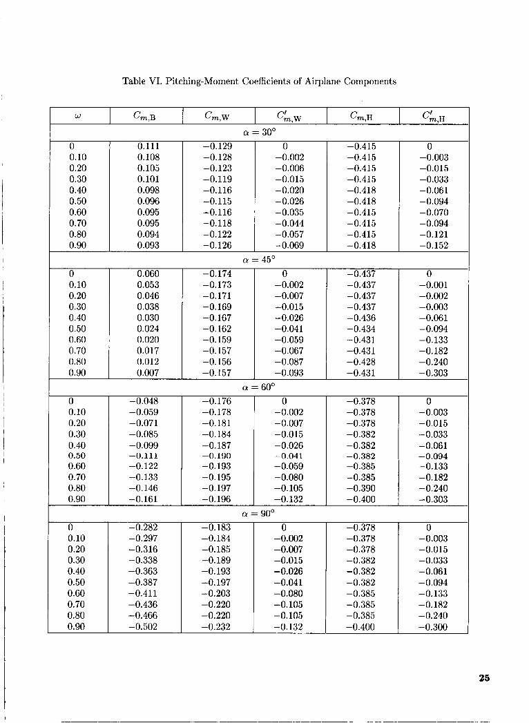
Table VI. Pitching-Moment Coefficients of Airplane Components
0 0.10 0.20 0.30 0.40 0.50 0.60 0.70 0.80 0.90
a = 30'
0.060 0.053 0.046 0.038 0.030 0.024 0.020 0.017 0.012 0.007
0 0.10 0.20 0.30 0.40 0.50 0.60 0.70 0.80 0.90
-0.048 -0.059 -0.071 -0.085 -0.099 -0.111 -0.122 -0.133 -0.146 -0.161
0.111 0.108 0.105 0.101 0.098 0.096 0.095 0.095 0.094 0.093
-0.176 0 -0.378 0 -0.178 -0.002 -0.378 -0.003 -0.181 -0.007 -0.378 -0.015 -0.184 -0.015 -0.382 -0.033 -0.187 -0.026 -0.382 -0.061 -0.190 -0.041 -0.382 -0.094 -0.193 -0.059 -0.385 -0.133 -0.195 -0.080 -0.385 -0.182 -0.197 -0.105 -0.390 -0.240 -0.196 -0.132 -0.400 -0.303
-0.129 -0.128 -0.123 -0.119 -0.116 -0.115 -0.116 -0.118 -0.122 -0.126
0 -0.002 -0.006 -0.015 -0.020 -0.026 -0.035 -0.044 -0.057 -0.069
Q = 45O -0.174 -0.173 -0.171 -0.169 -0.167 -0.162 -0.159 -0.157 -0.156 -0.157
0 -0.002 -0.007 -0.015 -0.026 -0.041 -0.059 -0.067 -0.087 -0.093
0 0.10 0.20 0.30 0.40 0.50 0.60 0.70 0.80 0.90
0 0.10 0.20 0.30 0.40 0.50 0.60 0.70 0.80 0.90
-0.415 -0.415 -0.415 -0.415 -0.418 -0.418 -0.415 -0.415 -0.415 -0.418
-0.437 -0.437 -0.437 -0.437 -0.436 -0.434 -0.431 -0.431 -0.428 -0.431
0 -0.003 -0.015 -0.033 -0.061 -0.094 -0.070 -0.094 -0.121 -0.152
0 -0.001 -0.002 -0.003 -0.061 -0.094 -0.133 -0.182 -0.240 -0.303
-0.282 -0.297 -0.316 -0.338 -0.363 -0.387 -0.411 -0.436 -0.466 -0.502
-0.183 -0.184 -0.185 -0.189 -0.193 -0.197 -0.203 -0.220 -0.220 -0.232
0 -0.002 -0.007 -0.015 -0.026 -0.041 -0.080 -0.105 -0.105 -0.132
-0.378 -0.378 -0.378 -0.382 -0.382 -0.382 -0.385 -0.385 -0.385 -0.400
0 -0.003 -0.015 -0.033 -0.061 -0.094 -0.133 -0.182 -0.240 -0.300
25
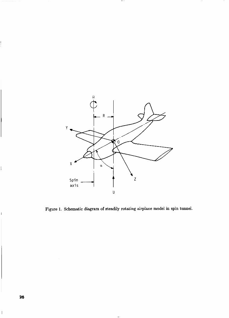
n
4 Spin 1 1 z a x i s
U
Figure 1. Schematic diagram of steadily rotating airplane model in spin tunnel.
26
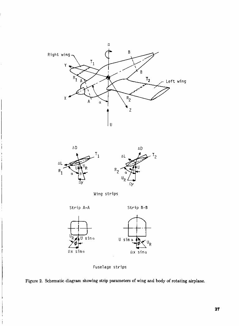
A D
Z
i, A D
fly
Wing s t r i p s
S t r i p A-A
U
S t r i p B-B
R x s i n a R X s i n a
Fuselage s t r i p s
Figure 2. Schematic diagram showing strip parameters of wing and body of rotating airplane.
27
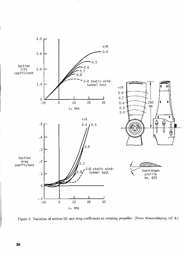
4.0
3.0 1 Sect ion
1 i f t c o e f f i c i e n t
r / R 0.4
2-D s t a t i c wind- tunne l t e s t
- 10 0 10 20 30
a, deg
r / R
Sec t ion drag
coef f i c i en t
-.l -10 0 10 20 30
a , deg
a Goet t ingen \ p r o f i l e
No. 625
Figure 3. Variation of section lift and drag coefficients on rotating propeller. (From Himmelskamp, ref. 9.)
28
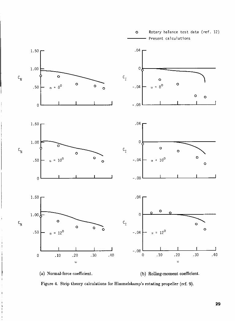
1.00
0 - -
1.50 r
cN 0
.50 a = l oo 0 -
0 2
1.50 -
cN
0 .10 .20 .30 .4@ w
(a) Normal-force coefficient.
o Rotary balance t e s t data ( r e f . 1 2 ) Present ca lcu la t ions
04
0 -.04 1 a = 8’
I 0 0
- .08 = .04
0
-.04
- .08
0
0 - a = l O 0
0
m o 4 r 0
-.04
0
0 a = 12 0
- .OB 3 0 .10 .20 .30 .40
0
(b) Rolling-moment coefficient.
Figure 4. Strip theory calculations for Himmelskamp’s rotating propeller (ref. 9).
29
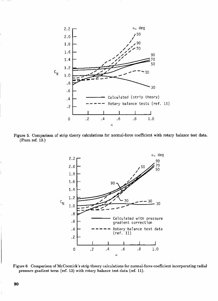
2 . 2 2.0 Ir
.6
.4
.2
a, deg
I 5 0 /
Calculated with pressure
----- Rotary balance t e s t data - gradient correction -
( r e f . 11)
I I I I 1 -
c N
1.8
1.6
1.4
1.2
1.0
.8
Calculated ( s t r i p theory) ----- Rotary balance t e s t s ( r e f . 11)
0 .2 .4 .6 .8 1.0 w
Figure 5. Comparison of strip theory calculations for normal-force coefficient with rotary balance test data. (nom ref. 13.)
cN
2.2
2.0
1.8
1.6
1.4
1.2
1.0
.8
90 70 50
30
Figure 6. Comparison of McCormick’s strip theory calculations for normal-force coefficient incorporating radial pressure gradient term (ref. 13) with rotary balance test data (ref. 11).
30
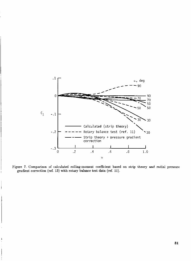
.1
0
cz -.l
-.2
- . 3
'\ Calculated ( s t r i p theory) - ----- Rotary balance tes t ( r e f . 11) '30
--- S t r i p theory + pressure gradient correction
0 . 2 .4 .6 .c 1.0 w
Figure 7. Comparison of calculated rolling-moment coefficient based on strip theory and radial pressure gradient correction (ref. 13) with rotary balance test data (ref. 11).
31
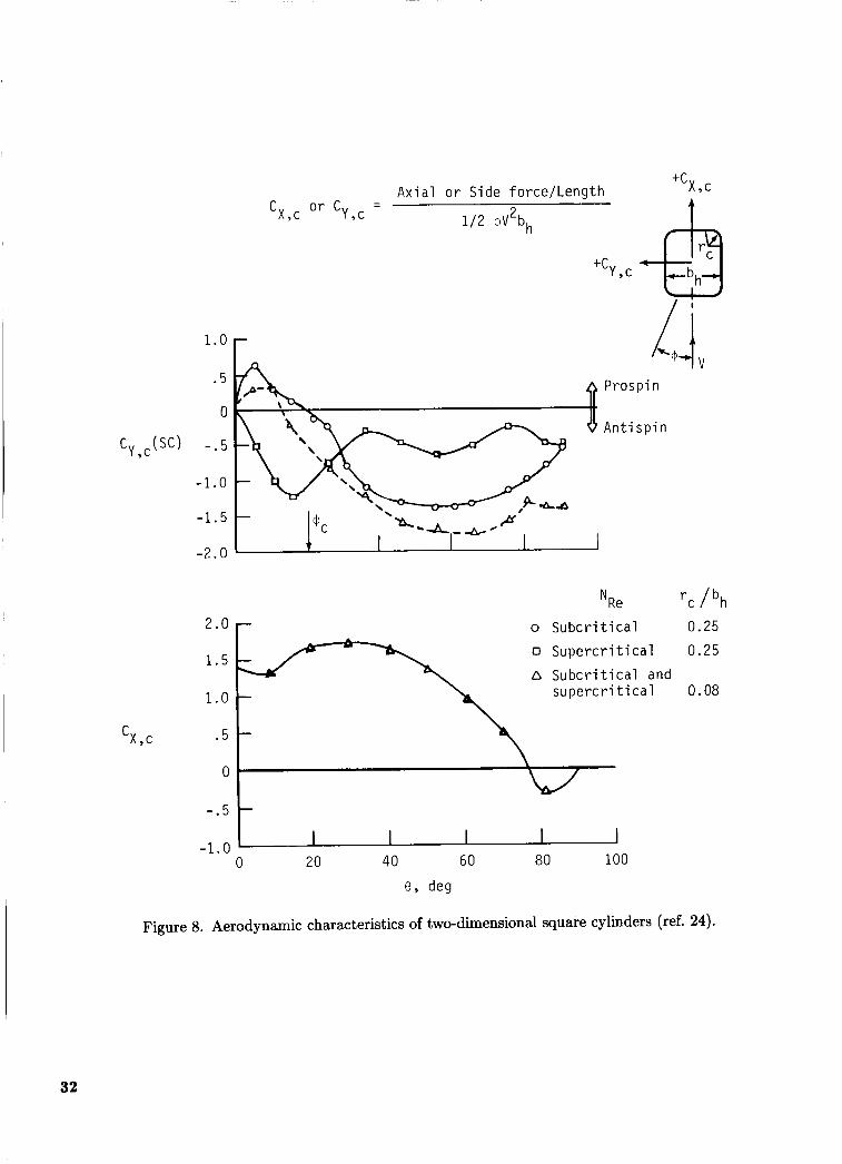
1.0
.5
0
cy ,c ( sc ) - .5
-1.0
-1.5
- 2 . 0
Re rc / b h 2 . 0 o S u b c r i t i c a l 0.25
o S u p e r c r i t i c a l 0.25 D S u b c r i t i c a l and
s u p e r c r i t i c a l 0.08
- .
1.0
.5
- - cx,c
- .5
-1 .0
-
I I I I 0 20 40 60 80 100
0 , deg
Figure 8. Aerodynamic characteristics of two-dimensional square cylinders (ref. 24).
I 32
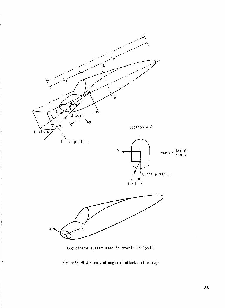
U cos B s i n CI
Sect ion A-A
y--ps U s i n B
t a n 4 =
B s i n a
t a n B s i n a
Coordinate system used i n s t a t i c a n a l y s i s
Figure 9. Static body at angles of attack and sideslip.
33
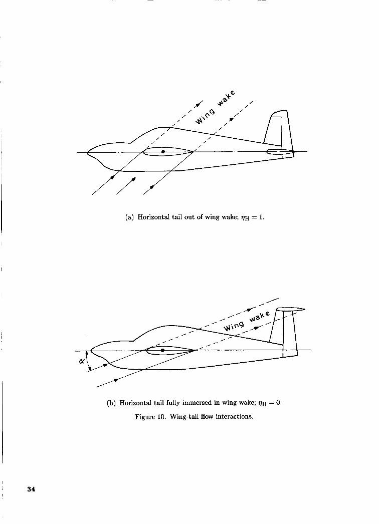
(a) Horizontal tail out of wing wake; T,IH = 1.
(b) Horizontal tail fully immersed in wing wake; 7~ = 0.
Figure 10. Wing-tail flow interactions.
34
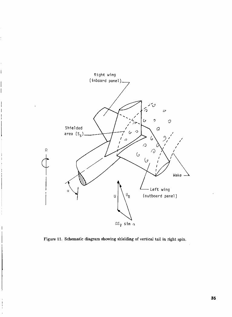
R i g h t wing ( i nboard panel ) 7
R
Figure 11. Schematic diagram showing shielding of vertical tail in right spin.
35
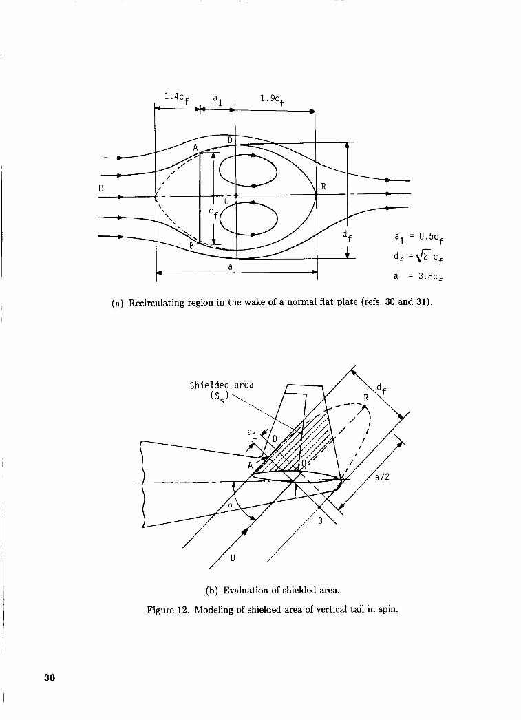
L
0. 5cf
@- C f
3 . 8 ~ ~
(a) Recirculating region in the wake of a normal flat plate (refs. 30 and 31).
/" / (b) Evaluation of shielded area.
Figure 12. Modeling of shielded area of vertical tail in spin.
36
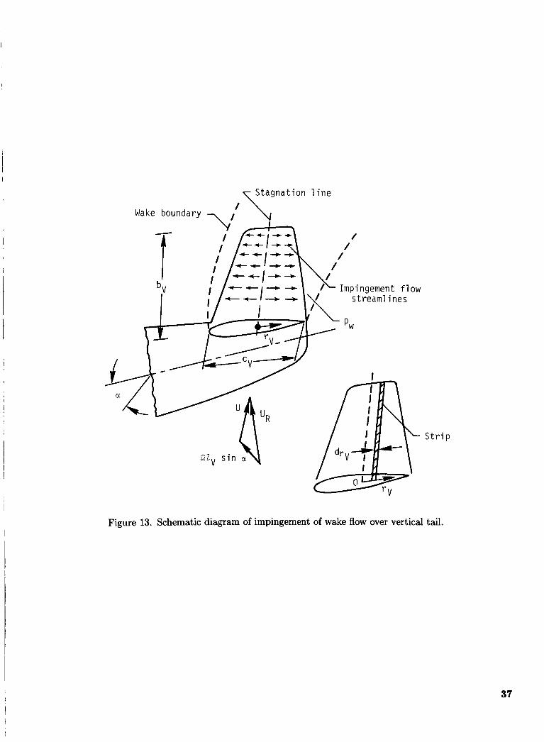
7 Stagnation 1 ine
Strip
Figure 13. Schematic diagram of impingement of wake flow over vertical tail.
37
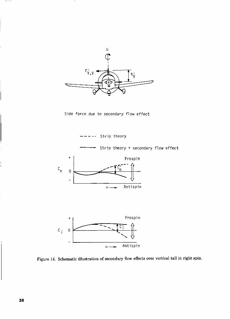
h
Side f o r c e due t o secondary f low e f f e c t
- - -__ S t r i p theory
- S t r i p t h e o r y + secondary f l o w e f f e c t
+ I Prospin
W- A n t i s p i n
Prosp in + I
W- A n t i s p i n
Figure 14. Schematic illustration of secondary flow effects over vertical tail in right spin.
30
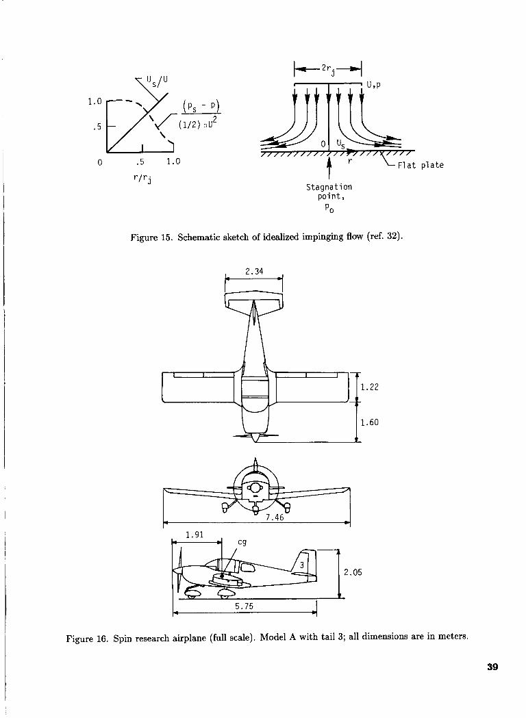
F l a t p l a t e t r S t a g n a t i o n
p o i n t , Po
Figure 15. Schematic sketch of idealized impinging flow (ref. 32).
1.22
1 .60
1.91 4 cq
5.75
Figure 16. Spin research airplane (full scale). Model A with tail 3; all dimensions are in meters.
39
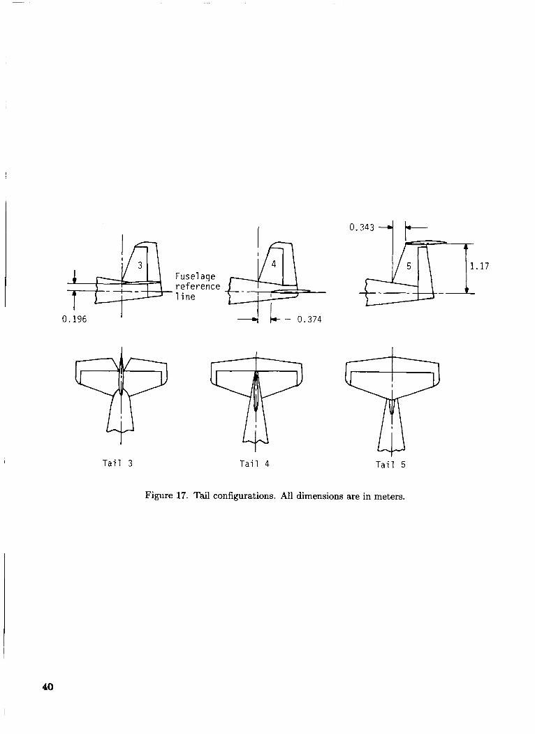
I
I
T a i l 3 T a i l 4
0.343 4
T a i l 5
. 17
Figure 17. Tail configurations. All dimensions are in meters.
40
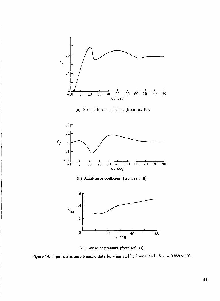
(a) Normal-force coefficient (from ref. 10).
-.21 1 1 1 I 1 I I I 1 1
-10 0 10 20 30 40 50 60 70 80 90 a, deg
(b) Axial-force coefficient (from ref. 10).
I I I 1 I 1 1 0 20 40 60
a, deg
( c ) Center of pressure (from ref. 33).
Figure 18. Input static aerodynamic data for wing and horizontal tail. N R ~ = 0.288 x lo6
41
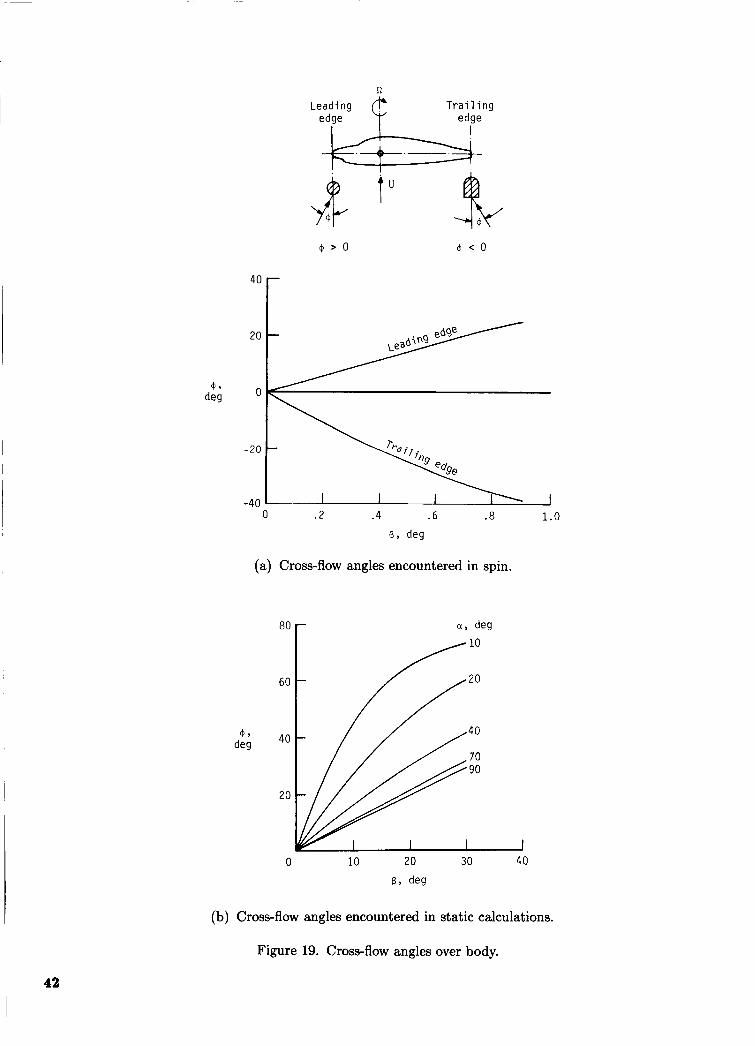
Trailing edge
Leading edge
0 .2 .4 .6 .8 1.0 B, deg
(a) Cross-flow angles encountered in spin.
60
40
20
0 10 20 30 40 B, deg
(b) Cross-flow angles encountered in static calculations.
Figure 19. Cross-flow angles over body.
42
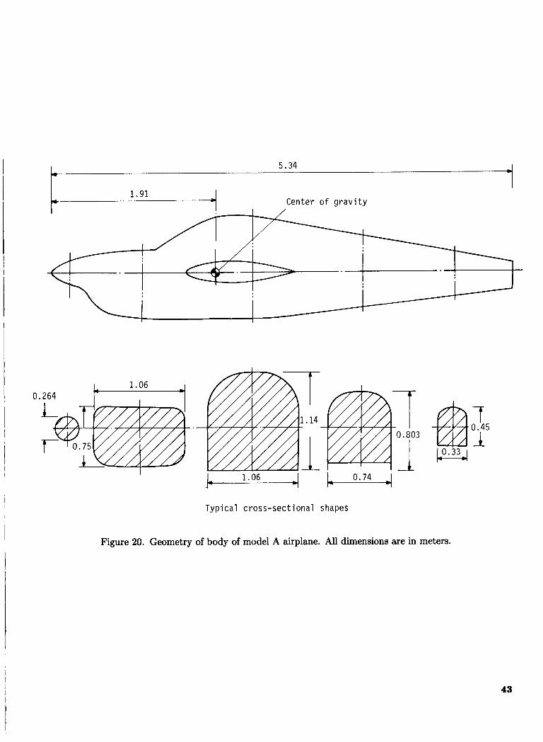
5.34 c
1.91 Center o f gravity
I
/
I
0.264 t 1.06
3
Typical cross-sectional shapes
Figure 20. Geometry of body of model A airplane. All dimensions are in meters.
43
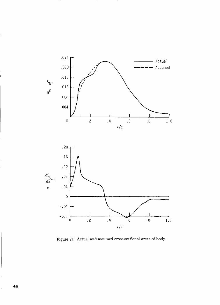
.024
.020
.016
.012 s B
2 m .008
.004
0
.20
.16
.12
dSB .08 - 
dx m .04
0
-.04
-.08
Actual Assumed
.2 . 4 .6 X I 2
. 8 1.0
0 .2 . 4 .6
x11 .8 1.0
Figure 21. Actual and assumed cross-sectional areas of body.
44
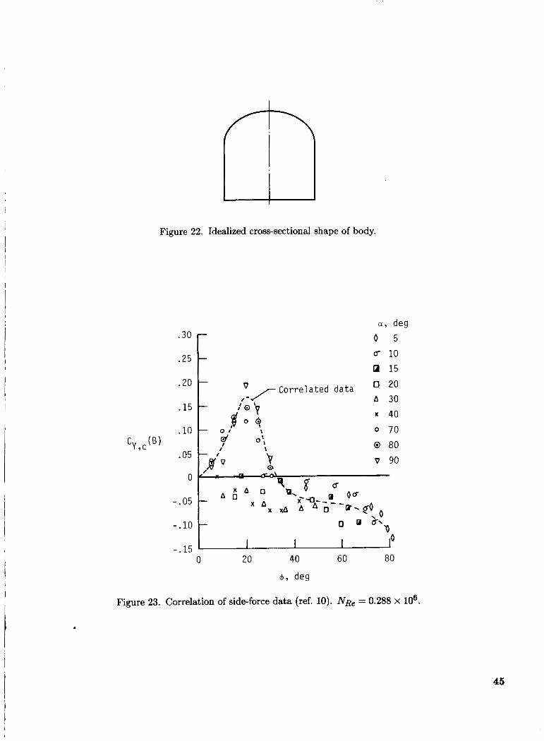
Figure 22. Idealized cross-sectional shape of body.
.30
.25
0 20 A 30
x 40
0 70
.20
.15 1 jb+ '-
.10 0 1
v~ C o r r e l a t e d d a t a
/ o ' v
-.15 0 20 40 60 80
( $ 3 deg
Figure 23. Correlation of side-force data (ref. 10). N R ~ = 0.288 x lo6.
45
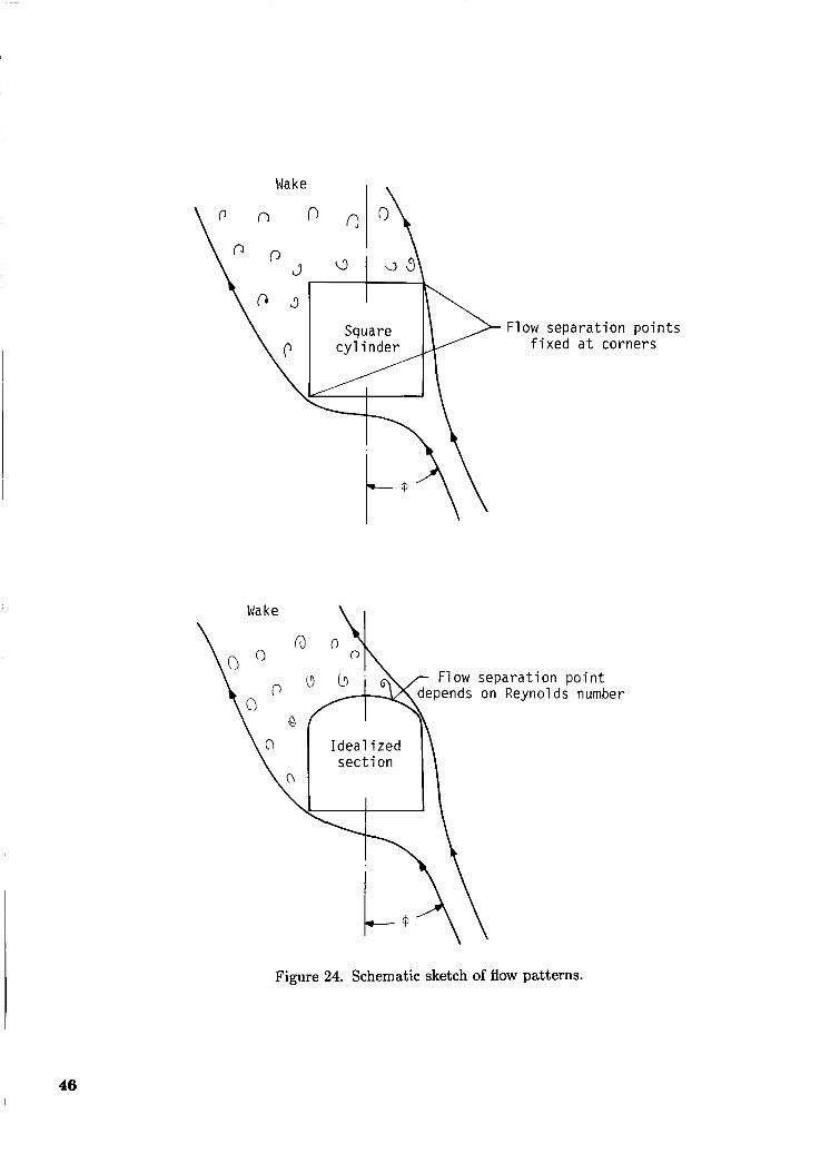
F l o w separa t ion p o i n t s f i x e d a t corners
Figure 24. Schematic sketch of flow patterns.
46
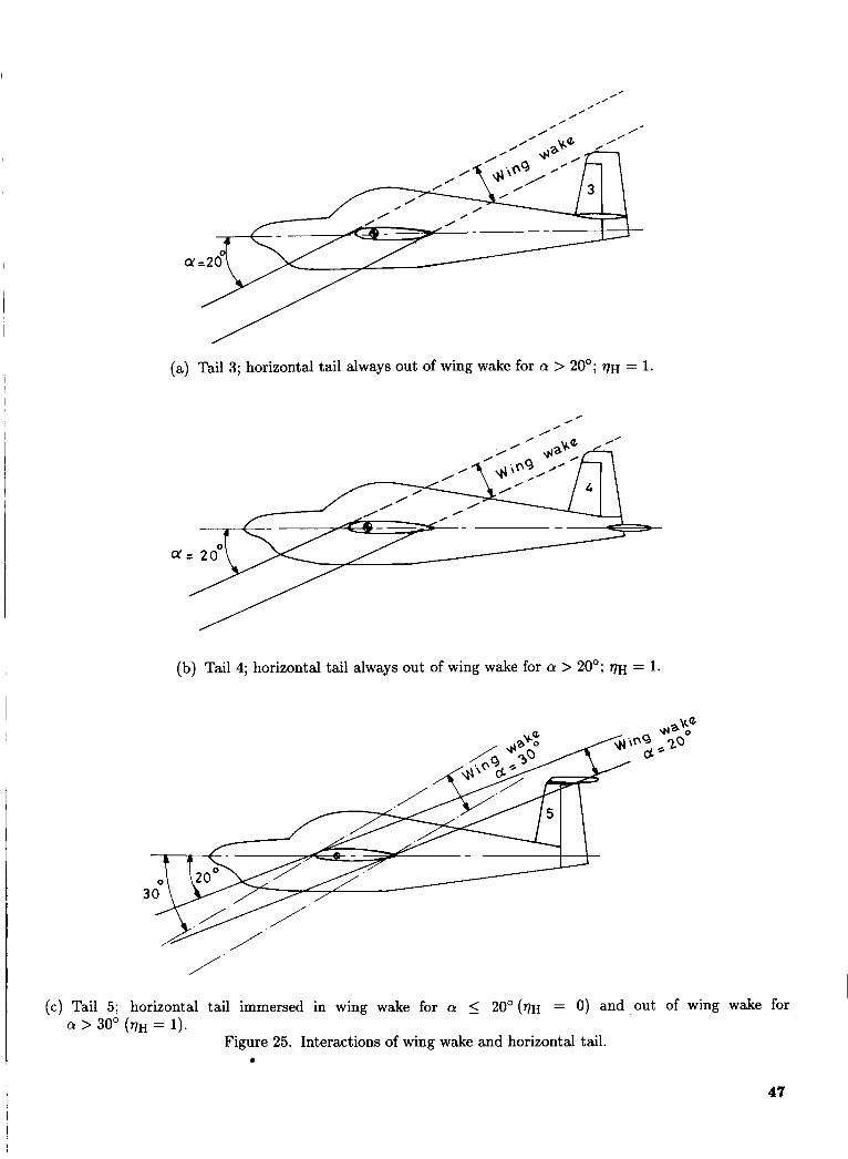
(a) Tail 3; horizontal tail always out of wing wake for (Y > 20°; VH = 1.
, , 0'
(b) Tail 4; horizontal tail always out of wing wake for (Y > 20'; VH = 1.
(c) Tail 5; horizontal tail immersed in wing wake for (Y 5 20° ( q ~ = 0) and ,out of wing wake for (Y > 30' (VH = 1).
Figure 25. Interactions of wing wake and horizontal tail.
47
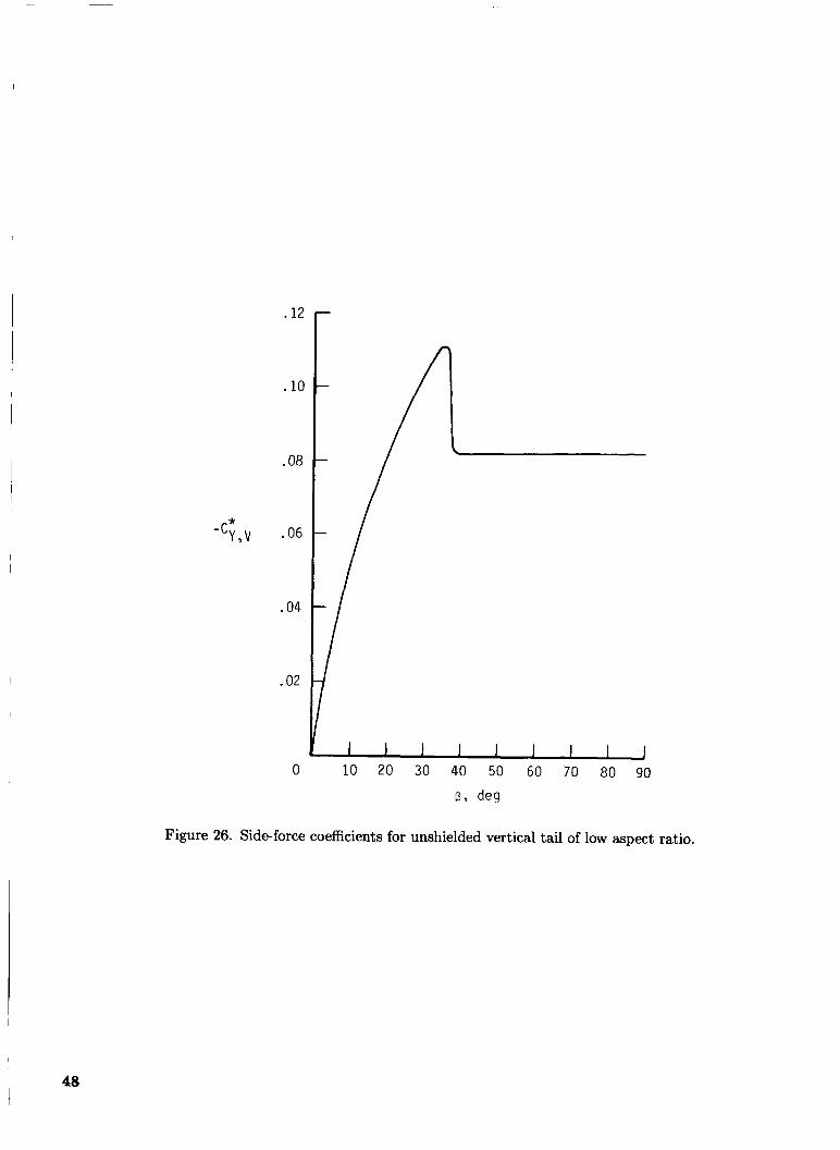
.12
.10
.08
-c;,v .06
.04
.02
0 1 1 1 J 1 1 1 1 J
10 20 30 40 50 60 70 80 90
B, des
Figure 26. Side-force coefficients for unshielded vertical tail of low aspect ratio.
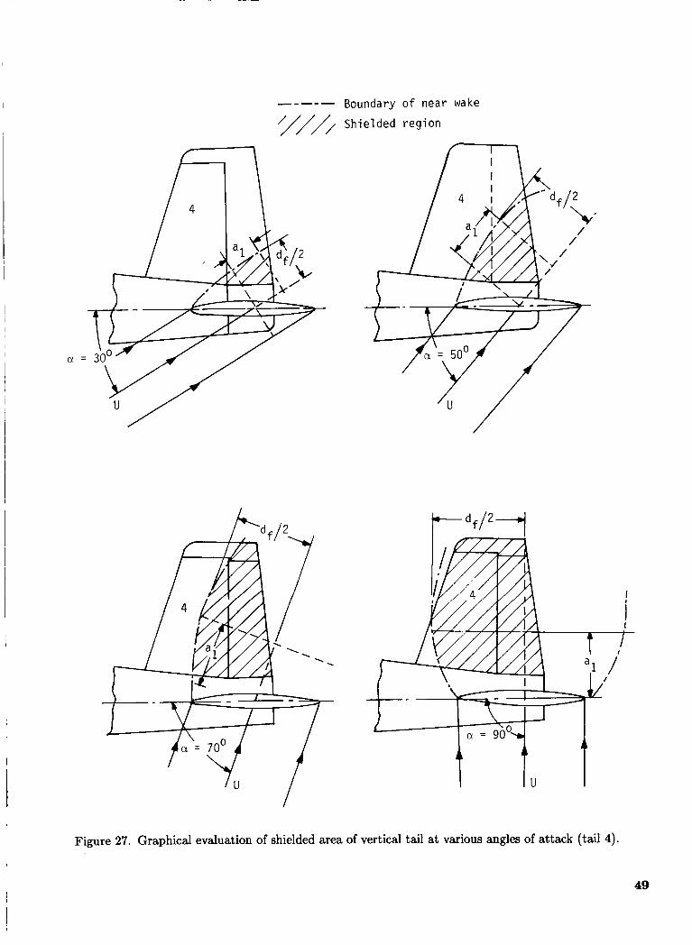
----A Boundary of near wake
'///, Shielded region
'" I Figure 27. Graphical evaluation of shielded area of vertical tail at various angles of attack (tail 4).
49
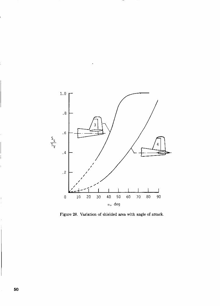
1.0
.8
.6
ss s V -
.4
.2
0
/ /
/ /
/ /
/
/ /
/ / /
/
Figure 28. Variation of shielded area with angle of attack.
50
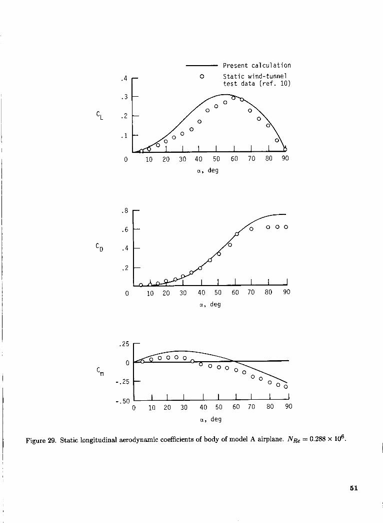
Present calculation
s 4 r 0 Sta t i c wind-tunnel t e s t d a t a ( r e f . 10)
. 3 -
cL
0 10 2 0 30 40 50 60 70 80 90
a, deg
c D
.8
.6
.4
.2
I
L 0 10 2 0 30 40 50 60 70 80 90
a, deg
-.50 0 10 20 30 40 50 60 70 80 90
a, deg
Figure 29. Static longitudinal aerodynamic coefficients of body of model A airplane. N R ~ = 0.288 x lo6. I
5 1
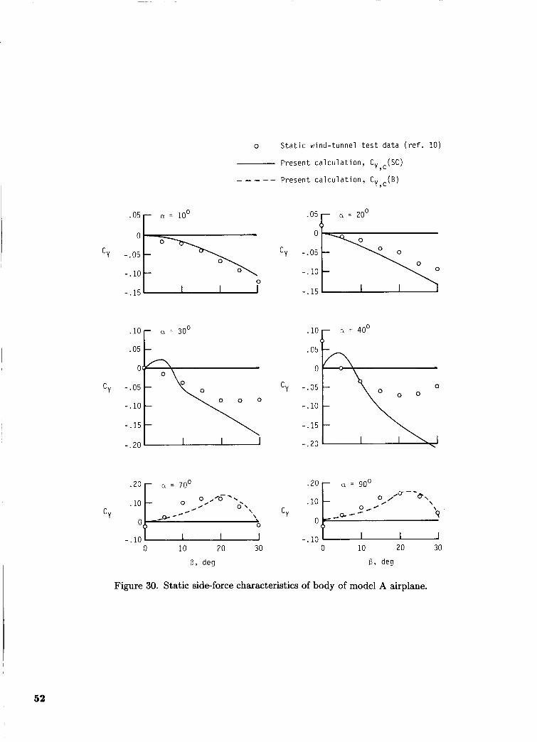
o S t a t i c wind-tunnel t e s t data ( r e f . 10)
Present ca lcu la t ion , C (SC) Y,c _ _ - - - Present ca lcu la t ion , C y , c ( B )
0
a = lo
-.15 u
0
‘”“b = 2o
-.05 0
-. 10
-. 15
.10
.05
0
Cy -.05
- . l o
-.15
- .20
- a = 30’
o \
C Y
0
’”b = 40 .05
0
- .05
- . l o
-.15
- . 20
L
- .10 0 10 20 30
B, deg
-. 10 , 0 10 20 30
8, de?
Figure 30. Static side-force characteristics of body of model A airplane.
52
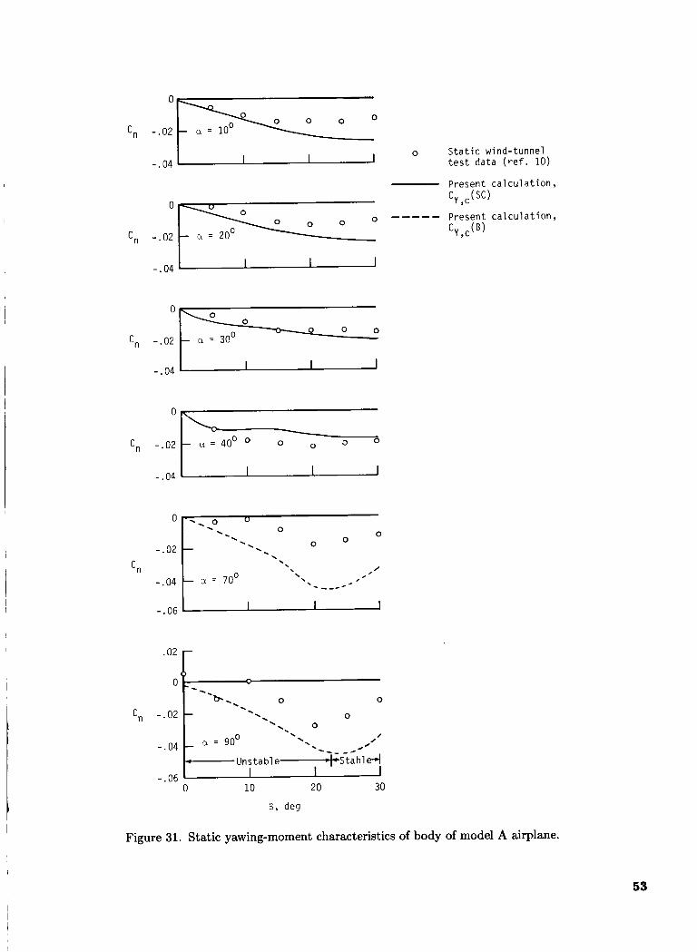
‘n
‘n
‘n
‘n
‘n
‘n
-.02 oc a = 10
-.04 3
-.02 ol a = 20
- .04 i
-.02 O l 0 a = 30
- .04 1
-.02 a = 40’
- .04
- .02
/ \ , . . ‘-----.
-.06 2 .02 r
n b
8 , deg
0 S t a t i c w ind- tunne l t e s t da ta ( r e f . 10)
Present c a l c u l a t i o n , cy ,c (sc)
C Y ,c(B)
----- Present c a l c u l a t i o n ,
Figure 31. Static yawing-moment characteristics of body of model A airplane.
53
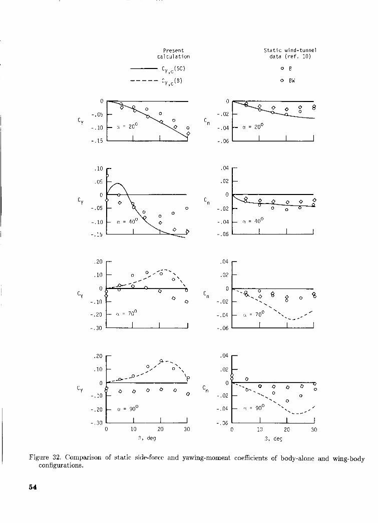
Present c a l c u l a t i o n
c y p c )
C Y , c @ ) -----
S t a t i c wind-tunnel d a t a ( r e f . 10)
O B
0 BW
- .05 -.02
-.IO c1 = 20 0 0 C Y
-.15 - .06
C Y
.10
.05
0
- .05
- . l o
- . 15
'n - .02 0
-.06 u
u 0 .02
cn o k
- . l o O O - .02 I I
/ \ . . / c _ *
-.20 1 CY = 70' -.04 1 CY = 70' '\
- .30 ' -.06 L
.20
.10
0 C"
- . l o
- .20
- .30 0 10 20 30
6. deg 0 10 20 30
B, deg
Figure 32. Comparison of static side-force and yawing-moment coefficients of body-alone and wing-body configurations.
54
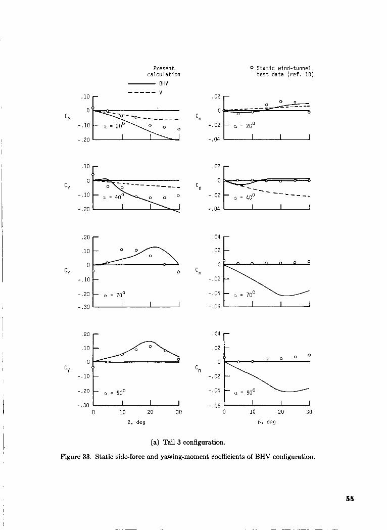
Present cal cul a t i on
- . l o
-.20
- .30
0 S t a t i c wind-tunnel t e s t data ( r e f . 10)
- 0 - = 70
1 I I -.06 I I 1
.04 2o r
.02
C Y - .02 :::: 1 a = go; , , -.04
-.30 - .06 0 10 20 30
R, deg
D 10 20 30
13, deo
(a) Tail 3 configuration.
Figure 33. Static side-force and yawing-moment coefficients of BHV configuration.
55
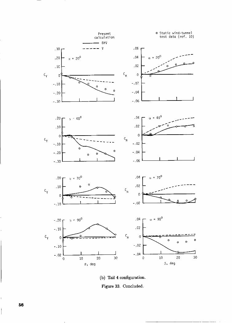
.30
.20
.10
CY
- ----- - _----
/ - a = 200 .04 - a = 20' , / /
-
0 -20r a = 40
- .O?
-.20 - - .04
- - - - -_____
'n
- -
-.02
- .04
.04 r = 700 0 .20 r ~1 = 70
- -
. l o p y cn .I LLOA --------- -----____ 0 s----
- . l o - .02
0 .04 r cx = 90
(b) Tail 4 configuration.
Figure 33. Concluded.
56 I
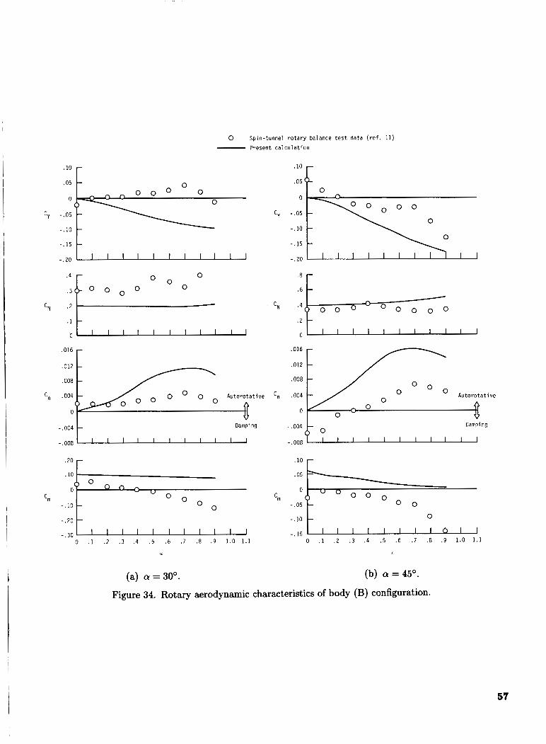
0 Spin-tunnel rotary balance test data (ref. 11) Present calculation
-.004 Damping () 0
- Damping -.004 - 1 1 1 1 1 1 1 1 1 1 1
.20
.10
0
-.IO
-.20
-.30
C",
w
- . l o - .05 \
() 0 o n
U " 0 (
U Q
0 0 O O 'm 0 0 0
-.05 - O O -
- . l o - 0 -
1 1 1 1 1 1 1 1 1 1 l - . I 5 1 1 1 1 1 1 1 1 0 1 1
(a) a = 30'. (b) (Y =45'.
Figure 34. Rotary aerodynamic characteristics of body (B) configuration.
57
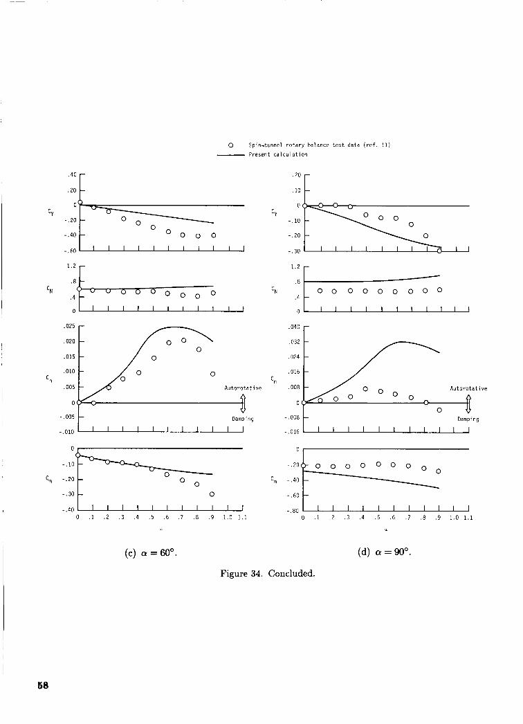
0 Spin- tunne l r o t a r y b a l a n c e t e s t d a t a ( r e f . 11)
- Present c a l c u l a t i o n
.40
.20
0
-.20
-.40
-.60
C Y
.20 - - - . l o -
C Y - O O O O -.20 -
- -
I l l l l l l l l l ~ - .30 I I I I I I I I
.008 Damping
,016 1 l 1 1 1 1 1 1 1 1 1
c, -.20 - .40
-.30 0 -.60 - -.40 I I I I I I I I I I I - .80 1 1 1 1 1 1 1 1 1 1 1
0 .1 .2 . 3 . 4 . 5 . 6 . 7 .8 . 9 1.0 1.1 0 .1 .2 . 3 . 4 . 5 .6 .7 .8 .9 1.0 1.1
w
(c) (Y =60°. (d) (Y =90°.
Figure 34. Concluded.
58
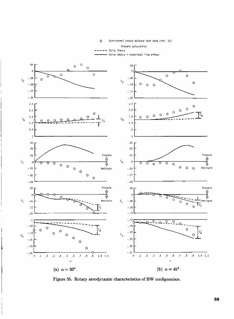
0 Spin-tunnel rotary balance test data (ref. 11)
Present calculation ----- Strip theory Strip theory + rotational f l o w effect
.03 - .03
.02
.01
‘n o
-.01 - 0 Antis pin -.01 0
-.02 - 0 -.02
-.03 -.03 0
CY
r
-
- Prospin
,
- 0 0 0 Antispin O O O O 0 0
-
0 -.04
-.08
.05 r v
0 0
-.16 I -.20 1
-.20
-.25 cnl
0 -.15
-.20 t 0 -.30 t h -.25 ’ ” -.35 ’
0 . I . 2 .3 .4 , .5 .6 .7 .E .9 1.0 1.1 0 .1 . 2 . 3 . 4 .5 .6 .7 .E .9 1.0 1.1
w w
(a) a = 30’. (b) a = 45O.
Figure 35. Rotary aerodynamic characteristics of BW configuration.
59
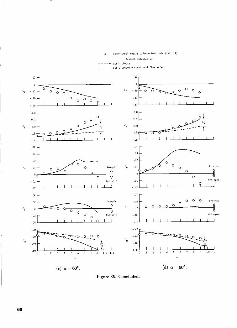
0 S p i n - t u n n e l r o t a r y ba lance t e s t d a t a ( r e f . 11)
Present c a l c u l a t i o n
----- S t r i p t h e o r y - S t r i p t h e o r y + r o t a t i o n a l f l o w e f f e c t
.lo r .10 r
c y - . l o 0 0 0 0
cy -.20 -.l:; o o r\
-.20 0
3.0 r 3.0 r
.04
.03
P r o s p i n
0 -.01 A n t i s p i n
-.02 I I I I I I I I I I I
.04 r .o: 1 ~ ob. P r T i n
A n t i s p i n
C l
0 - .02
::.I;;l --_ , -.40
-.50
cnl
i 0 .1 .2 ,3 .4 .5 .6 .7 .8 .9 1.0 1.1
( c ) Q = 60'.
'n
1.0 1 1 1 1 1 1 1 1 1 I I
.04 r
P r o s p i n
0
.05
c - 0
-.05 A n t i s p i n
cm
T -1.00
0 .1 .2 . 3 .4 .5 .6 .7 .E .9 1.0 1.1
w
(d) a=90° .
Figure 35. Concluded.
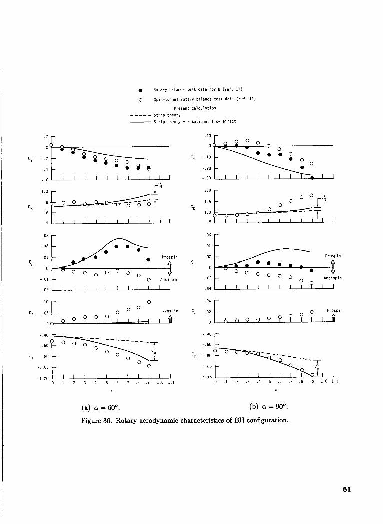
0
Rotary balance t e s t data f o r B ( r e f . 11)
Spin- tunnel r o t a r y balance t e s t data ( r e f . 11)
Present c a l c u l a t i o n
----- S t r i p theo ry - S t r i p theo ry t r o t a t i o n a l f l o w e f fec t
.04
c1 .02
0
cy - .2 -.4 O p 3 T - F 0 8 8
- Prospin - ? O O
h b o o O ?
- . 6 I I I I I I I I I I I rci
i n , - 1
'n
.03 -
.02 -
-.01 - 0 A n t i s p i n
.03 -
.02 -
.01 - 0
-.01 - 0 A n t i s p i n
.10 r 0
0 0 0 Prosp in
1 ! 1 I
-.40
- .60 -----_
cm -.a0
-1.ou
-1.20 1 1 1 1 1 1 I I 1 I l 0 .1 .2 . 3 . 4 .5 .6 .7 . 8 .9 1.0 1 . 1
w
(a) a = 60'
. l o I-
C" - . l o
-.20
- .30
2.0 r
.06 r Prospin
A n t i s p i n I V h
-.60 - . 4 0 L- -1.00
-1.20 0 . 1 . 2 .3 .4 .5 .6 .7 .8 .9 1.0 1.1
w
(b) a =90°.
Figure 36. Rotary aerodynamic characteristics of BH configuration.
61
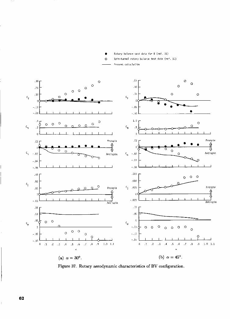
0 Rotary balance t e s t data f o r @ ( r e f . 11)
0 Spin- tunnel r o t a r y balance t e s t data ( r e f . 11)
- Present c a l c u l a t i o n
0 . l o .20 - 0
.10 - 0 .05 0 0
0 - 0
0 0 -
1.0 0 .4 0
0 0 1 1 1 1 1 1 1 1 1 1 1
O O O O CN . 5 o o o o
CN .2
I l l l l l l l l l j - - v u - "
- . l o
- .20
- .02 '03 1
- .05
- . l o ,
- -
1 1 1 1 1 1 1 1 1 1 ~ 0
LZ .01 0 o o O Prospin
- OQ
u CI
-.05
-.01 A n t i s p i n
- o o o 0 0
1 1 1 1 1 1 1 1 A 1 1
.15 r
0 .'l .2 .3 . 4 .5 .6 .7 .8 . 9 1 . 0 1 . 1
w
.015 r 0 0 0
-. 005 A n t i sp in
. l o r
- . l o
-.15 l l I 1 1 1 1 ~ ~ ~ 1 0
0 , I .2 . 3 . 4 .5 . 6 .7 . 8 . 9 1.0 1.1
w
(a) a =30°.
Figure 37. Rotary aerodynamic characteristics of BV configuration.
(b) a = 45'.
62
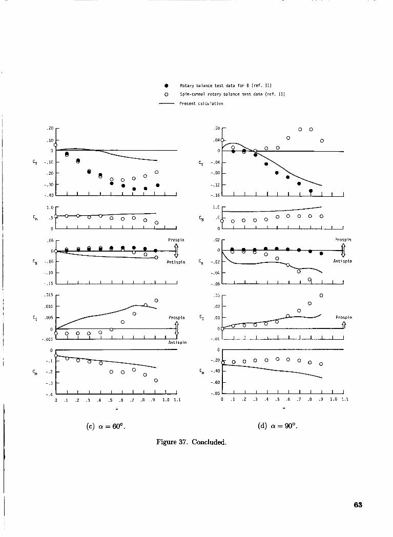
.IO '"6 O -
cy - . l o
0 Rotary balance t e s t data f o r B ( r e f . 11)
0 Spin-tunnel r o t a r y balance t e s t data ( r e f . 11)
- Present c a l c u l a t i o n
8 - 8
CN . 5
Prospin
- . 1 5
( 7 0 0 0 o 0 O O 0 0
,015
,010
CI ,005
0
-. 005
r 0
Prospin
Antispin
0 1
-.3 t 0
-.41 I I I I ' ' I I I J
0 .1 .2 .3 . 4 .5 .6 .7 .8 .9 1.0 1.1
W
(c) 0 = 6oo.
0 0 .08 r
CY
- . 1 6 c
.02 t 0 0
Ct .01 - Prospin
0 D
-.80 -.60 t L - L u L u 0 .1 .2 .3 . 4 .5 .6 .7 .8 .9 1.0 1.1
W
(d) a=9O0.
Figure 37. Concluded.
63
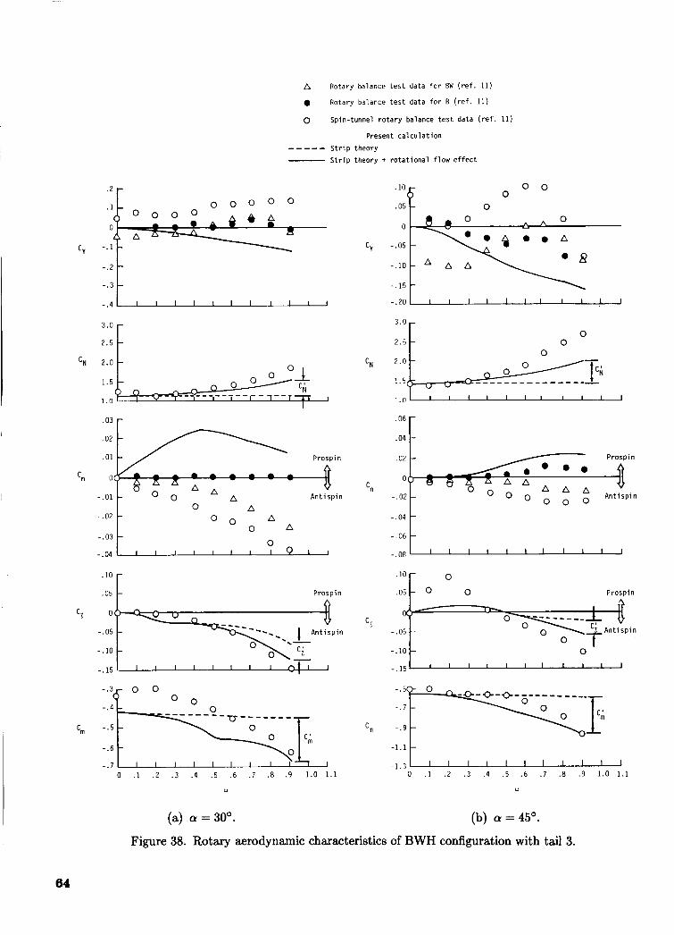
A
0
.02
O()
-.02
- . 3 -.* 1
- Prospin
g -
.03 r
Rotary balance t e s t data f o r Bk' ( r e f . 11)
Rotary balance t e s t data f o r B ( r e f . 11)
Spin-tunnel r o t a r y balance t e s t data ( r e f . 11)
Present c a l c u l a t i o n
S t r i p theory S t r i p theory + r o t a t i o n a l f l o w ef fect
L
A A A -.01
O O A n t i spin
0 A 0 0 A
0 A ,. -.03 U
-.04 I I I I I l l 1 0 1 1
.05 'lo c Prospin
CZ
-. 15 l l c w
0 .1 . 2 .3 .4 .5 .6 .7 .8 .9 1.0 1.1
w
(a) a = 3 0 ° .
.10 0 0
.05 0 - 0
-.lo - A A A
-.15 -
2.5 3'0 1 0 0
.06
.04
-.04 t -.OB -.06 5
0 :x 0 0 Prospin
-.05
-1.1 1 -1.31 I I I I ' I 1 I I I J
0 . 1 .2 .3 .4 .5 .6 .7 .8 .9 1.0 1.1
w
(b) a = 45'.
Figure 38. Rotary aerodynamic characteristics of BWH configuration with tail 3.
64
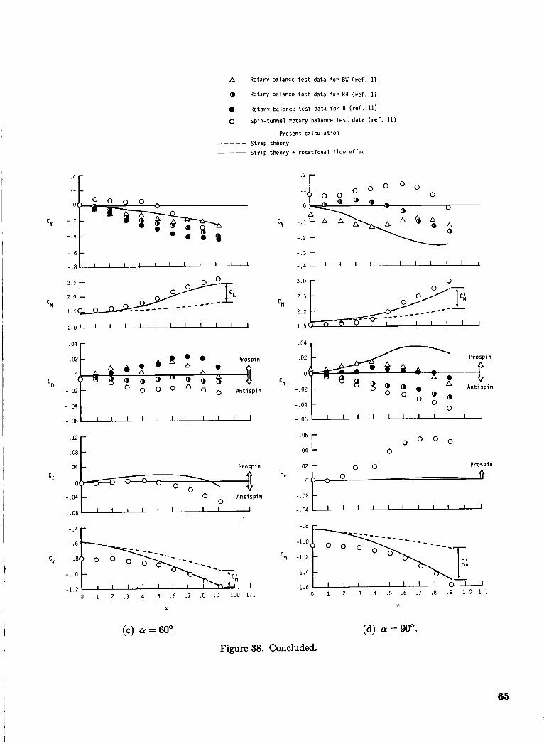
.2 . 4 [I
A Rotary balance t e s t data f o r BW ( r e f . 11)
0 Rotary balance t e s t data f o r BH ( r e f . 11)
0
Rotary balance t e s t data f o r B ( r e f . 11)
Spin-tunnel r o t a r y balance t e s t d a t a ( r e f . 11)
Present c a l c u l a t i o n
----- S t r i p theory - S t r i p t h e o r y + r o t a t i o n a l flow e f f e c t
2.0
1.5
.04 r .02 -
-.02 -
-.04
-.06 1 1 1 1 1 1 1 1 ~ ~ 1
.12
.04 Prospin
-.04
- .08
0 .1 .2 . 3 .4 .5 .6 . 7 .8 .9 1.0 1.1
w
-.2 - -.3
- . 4 I I I I I 1 1 1 ~ ~ L
3.0 r 0
.04 -
.02 - Prospin
0
-.02 - -.04 0
-
::: Prospin
-.02
-.04
-1.0
-1.4
J
w
(dl a =90°. (c) a = 6oo.
Figure 38. Concluded.
65
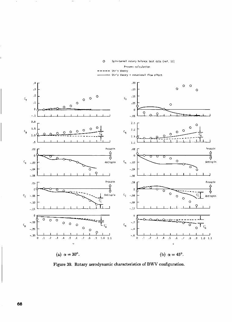
0 Spin- tunnel r o t a r y balance t e s t data ( r e f . 11)
Present c a l c u l a t i o n ----- S t r i p theo ry
S t r i p theory + r o t a t i o n a l f l o w e f f e c t
.4 - .zn
. 3 - .15
0 .10 .2 -
* I - 0 .05 0 0 C Y CY
0 0 (,-$U
-.l I I I I I I I I I I I -.05
- 0 0
0 - 0
-
0 0 -
o y 0 o l h i ! I I A
Prospin
- - - -_ -._ 1 A n t i s p i n -.05
-.lo
-.15 T
-.2
C Z
- n - c, O 0 T c ; ,
1 1 1 1 1 1 1 1 1 1 J
.04 r Prospin
-.OR 0
-.12 I I I I l l I l P l I
w w
(a) a =30°. (b) a=45'.
Figure 39. Rotary aerodynamic characteristics of BWV configuration.
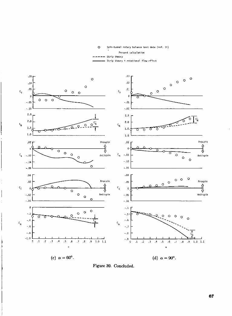
0 Spin-tunnel r o t a r y balance test data ( r e f . 11)
Present ca l cu la t ion ----- S t r i p theory - Strip theory + ro t a t iona l flow e f f e c t
0 .10 .I5 [:
-.05
- . lo ' . 2.5 I
1.0 I
.02 r Prospin
0 -.06
.04 - Prospin
0 Antispin 0
-.02
-.04
- 0
- . 4
- . 6
-1.0 ! 0 .1 .2 . 3 .4 .5 .6 . 7 .8 .9 1.0 1.1
.03
.02 0 o o
0
-.01
-.02 L
1.0 I
Prospin
-.05
0
-.15
.io r Prospin
-.05 1 - A n t i spin
- . lo ' -.4 r
w
(c ) cr = 6oo.
Figure 39. Concluded.
w
(d) cr = 90°.
67
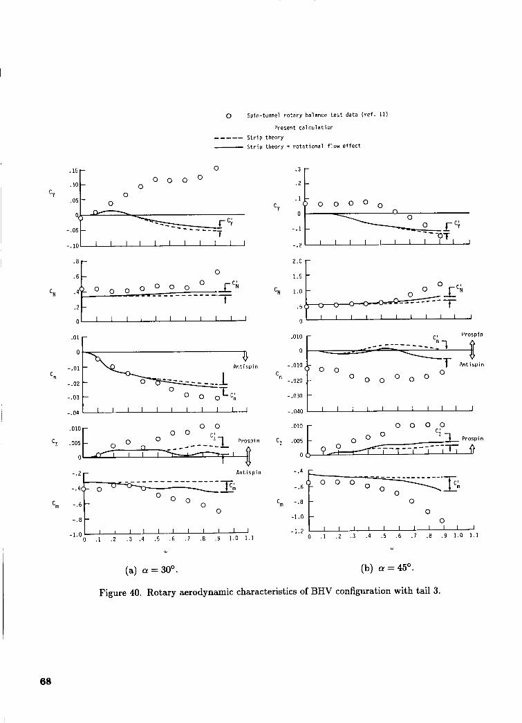
0 Spin-tunnel r o t a r y balance test data ( r e f . 11)
Present ca l cu la t ion ----- S t r i p theory - S t r i p theory t ro t a t iona l flow e f f e c t
cz .005
0 .15 0 0 0 0
0 0
0 .05 CY
0 0 0 -
O( -
-.05 -
.8 .6 c 0
.ol r A n t i sp in
‘n -.02
-.03
-.04
.010 - 0 0
0 c~ .005 0 0 0
-
- . 4 - . * ~ ~ - ~ ~ - ~ ~ ~ ~ - ~ - ~ ~ ~ t i , p i n
cm -.6
- .8
-1.0 0 .1 . 2 . 3 . 4 . 5 .6 . 7 .8 .9 1.0 1.1
w
(a) a =30°.
. 3
. 2 F 0
-.l
-.2
CY
-.n3n
- .040 I l l l l l l l l l l
.010 r 0 0 0 - 0
cm -1.2 -1 .o 3 0 .1 .2 . 3 . 4 . 5 .6 . 7 .8 .9 1.0 1.1
w
(b) a = 4 5 O .
Figure 40. Rotary aerodynamic characteristics of BHV configuration with tail 3.
68
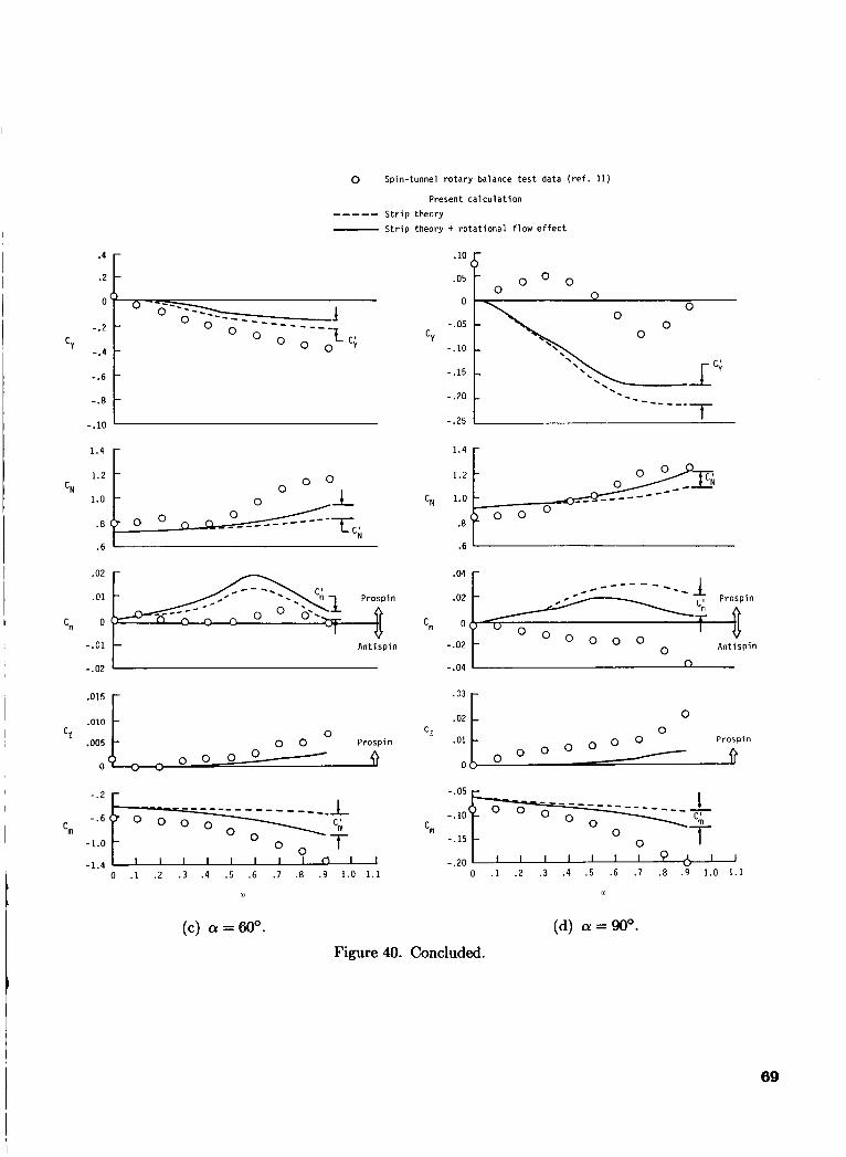
0 Spin-tunnel rotary balance tes t data (ref . 1 1 )
Present calculation ----- Strip theory - Strip theory + rotational flow ef fect
.4
.2
O Q
-.2
-.4
-.6
-.a
- . lo
CY
- -
1 0 0 0
0 - -- 0-
O 0 - - - - - 0 0 - - - - - _ _ _
-t c; - -
- -
*lo 6 .05
0
-.05
- . l o
-.15
-.20
-.25
CY
1.4
1.2
1.0 CN __-- _____- - - - 1.0
0 _ _ _ _ _ _ _ - -----
_ _ - - - - .02 -
Antispin 0 0 0 0 - .01 - Anti s p i n -.02
-.02 -.04
w w
(c) a = 6oo. (d) a =90°.
Figure 40. Concluded.
69
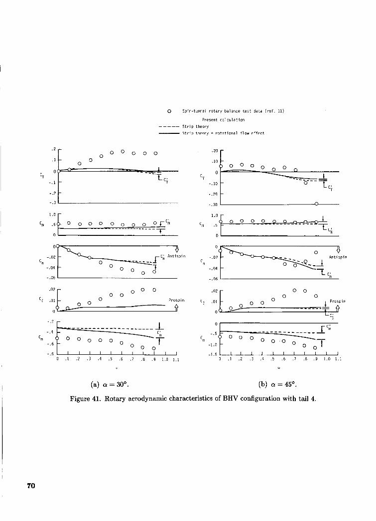
0 Spin-tunnel r o t a r y balance t e s t data ( r e f . 11)
Present c a l c u l a t i o n
----- S t r i p theory
- S t r i p theory + r o t a t i o n a l f l o w e f f e c t
-.3 -.2 * c; A n t i s p i n A n t i s p i n
'n -.04 -.04 0 0 -.06
.o* r 0 0 0 0
.02 f- - 0 0 0 0 "
D IPrT in 0 C L .01 0 0
0 Prospin e ----- cz .01
0 0 c;
- . 2
'rn - . 4 f = = ? ? + , , cm-;:::
-.6
-.8 -1.5 0
0 .1 .2 . 3 .4 .5 .6 . 7 .8 . 9 1.0 1.1 0 .1 .2 . 3 .4 .5 .6 . 7 .8 .9 1.0 1.1
w 0
(a) a =30°. (b) a = 4 5 O .
Figure 41. Rotary aerodynamic characteristics of BHV configuration with tail 4.
70
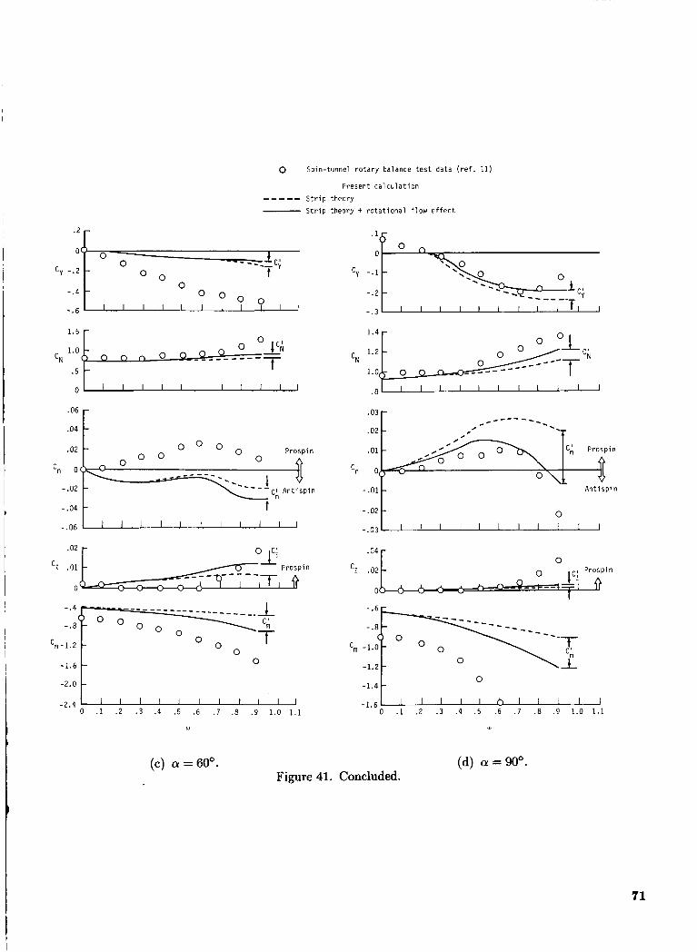
Q Spin-tunnel r o t a r y balance t e s t data ( r e f . 11)
Present c a l c u l a t i o n
----- S t r i p theory - S t r i p theory + r o t a t i o n a l f low e f fec t
.06
.04
.02
'n
-.02
-.04
.1
O n
c -_ _-- - - - - .03 c , - .02 - -.
- Prospin C,', Prospin
, . 0 0 0 0
ci A n t i s p i n -.01 - A n t i s p i n o(<
-
0 - .02 - -
1 1 1 1 l 1 1 1 1 1 1
-.6 ' I l l l 1 1 1 7 1 1 I I I I I I I T 1 1 '
-.06 -.03 I I l l l l l l l l l
-1.4
w w
0 -
(c) a = 60'. (d) a = 90'. Figure 41. Concluded.
71
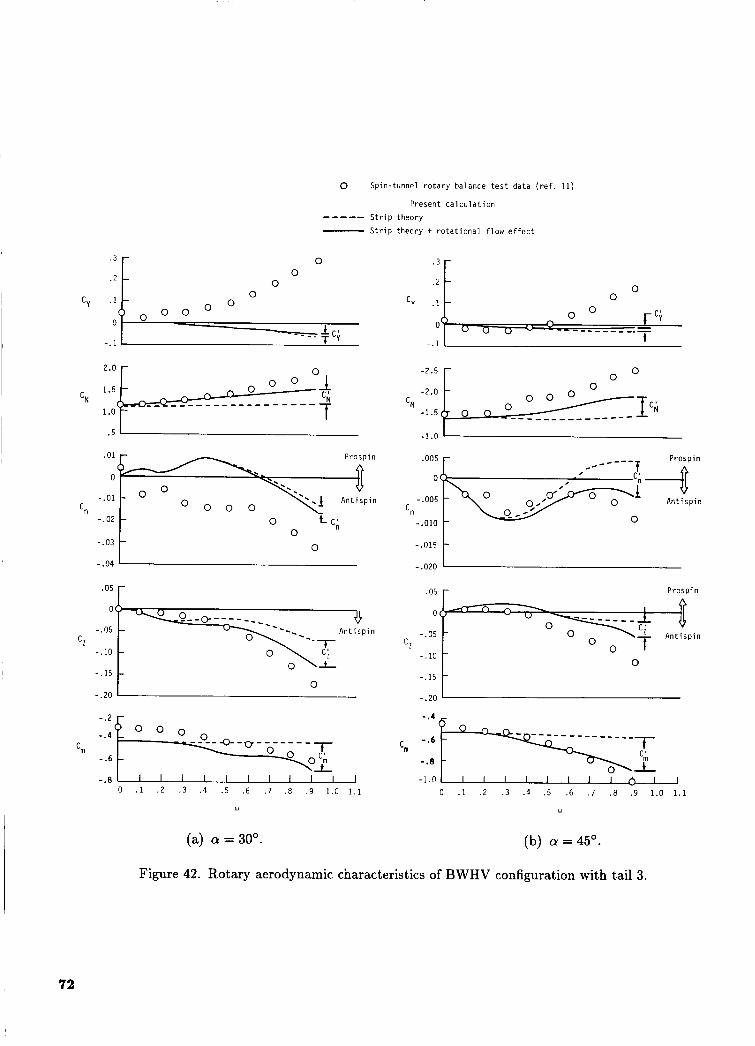
0 Spin-tunnel r o t a r y balance t e s t data ( r e f . 11)
Present c a l c u l a t i o n
----- S t r i p theory
S t r i p theory + r o t a t i o n a l f l o w e f f e c t
Prospin .005
-.005 0 'n 'n
-.010
-.015
-.02 - -.03 -
0
-.04 -.020
0 0
0
- Prospin
3 3 - 0 0,. 23' O O I Ant i sp in
0 Q - 0 - -
0
cy -. . l ~ 1
.05
0
-.05
-.IO
- . 15
-.20
CZ
U J
- .05 - Prospin
I
,$ - - - - - _ _ _ 0 0c-n 2 > - A n t i s p i n -.05 - 0 >+ 0 , n i p i n
C l 0 - . l o - - . I 5 - -.20 .
- 0 -
0
. 5 I
3r
- . I I
o o -2.5 r
-1.0 I
(a) Q =30°. (b) Q = 4 5 O .
Figure 42. Rotary aerodynamic characteristics of BWHV configuration with tail 3.
72
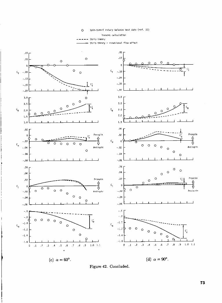
0 Spin-tunnel r o t a r y balance t e s t data ( r e f . 11)
Present c a l c u l a t i o n
----- S t r i p theory - S t r i p theo ry + r o t a t i o n a l f low e f fec t
.02
cn 0''
0 0
_.---- ------i c;I Prospin -
0 77
I I I I I I I I - - L I I - _ - . lo - -.15 - -.20
-.04
3.0 r 0
A n t i s p i n
- l 1 1 1 1 I I I I
1.5
-.04
Prospin
-.02 C"
- 0 0 0
A n t i s p i n
Prospi n
0 0 CZ
-.02 A n t i s p i n
-1.0
-1.2 'rn
0 -1.4 L 0
0 -1.6 1 1 1 1 1 1 ~ ~ ~ ~ J
0 .1 .2 . 3 . 4 . .5 .6 . 7 .8 .9 1.0 1.1
(c) Q = 60'.
3.5 r CN 2.5
2.0
1.5
.04 r I
" o o o o Ant i sp in -.02 1 0
-.04 1 0 0
-.06 1 1 1 1 1 1 1 1 1 1 1
0 O O 0
'rn
0 - -1.4
-1.6
0 .1 .2 . 3 .4 .5 .6 . 7 .8 . 9 1.0 1.1
w
(d) Q = 90'. Figure 42. Concluded.
73

0 Spin- tunnel r o t a r y balance t e s t data ( r e f . 11)
Present c a l c u l a t i o n
----- S t r i p theory - S t r i p theory + r o t a t i o n a l f low e f fec t
C Y
CN
'n
CZ
'rn
0 0
0
0
- .I t
0
0
0 0
0
2.5 3.0 [I 0 0
1.0 I
"
-.IO -
-.20 t -.301
O 1 - . 2 t
----- - - _ _ _ _ _ -.E
- .E 0 . I . 2 .3 .4 .5 .6 .7 .E .9 1.0 1.1
w
(a) Q =30°.
.05 r Prospin
- . l o 0
-.I5 0
- . 4 r
0 -1.0
-1.2 I l l I l l I I b l 1 0 . 1 . 2 . 3 .4 . 5 .6 . 7 .E .9 1.0 1.1
(b) a = 4 5 O .
Figure 43. Rotary aerodynamic characteristics of BWHV configuration with tail 4.
74
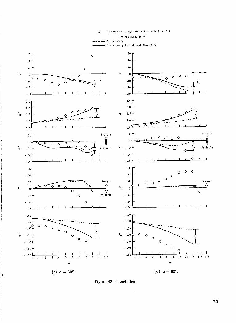
0 Spin-tunnel r o t a r y balance t e s t data ( r e f . 11)
Present c a l c u l a t i o n
----- S t r i p theo ry - S t r i p theo ry + r o t a t i o n a l f l o w e f fec t
.06 - .M
.04 - .04
Prospin .02
.10 I 0 :: f 0 .l
- - 0 0 0 0
Prospin 0 -
0 Ant i sp in -.02 -.02
-.04 - 0 -.04
-
-.60 - - . 5 0 -
-.EO -
T -1.00 -
cm -1.20 0 0 0
-1.40 P - cm -1.10 -
-1.30
-1.50
-
- 0
-1.60 - I l l l l l l l l l l I I l l I 1 1 0 1 I I
-1.70 -1.80 0 , 1 .2 .3 . 4 .5 .6 .7 .8 . 9 1.0 1.1 0 .1 . 2 . 3 .4 . 5 .6 .7 .8 .9 1.0 1.1
w w
c; - -
(c) a = 6oo. (d) a = 90°.
Figure 43. Concluded.
75
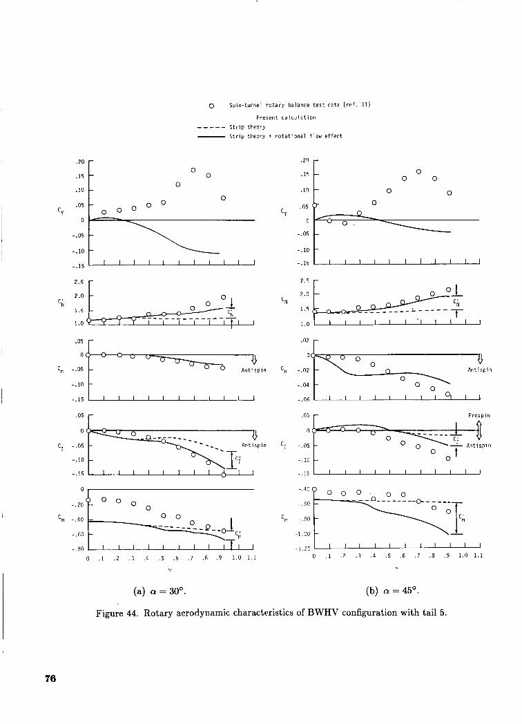
0 Spin-tunnel r o t a r y balance t e s t data ( r e f . 11)
Present c a l c u l a t i o n
----- S t r i p theory - S t r i p theory + r o t a t i o n a l f low e f fec t
0 0
0
0 .05 0 0
CY o o o C V
0 0 0
0 0
0
-.05
- . lo
-.15 I I I I I I I I I I J
2 - 5 [ ~ ~ ~ ~ I cN :::I: ~l I c o t l , 2.0
1.5 T 0 _ _ _ _ _ _ _ _ - - - - - - - - - 0 1.5
1 .o 1.0
c i CE. - - - - - _ _ _ _ _ _ _ - --
.02 - oc
0 u A n t i s p i n cn -.02 - 0 Ant i sp in
0
I I I I I I I 1 0 1 I I -.04 - 2
-.15 -.06
.05 .05 - Prospin
1 C!
A n t i s p i n c; - .05 - A n t i s p i n
- . l o - 0
Cz -.05
-.15 - . l f i - ' I I I I I I I I I I
-.20
-.40 0 0 - , RO
- .60 -1 .00
-1.20 -.80 0 .1 . 2 . 3 . 4 . 5 .6 .7 .8 .9 1.0 1.1 0 . 1 . 2 . 3 . 4 , 5 .6 .7 .8 .9 1.0 1.1
I(
(a) a = 30'. (b) a=45' .
Figure 44. Rotary aerodynamic characteristics of BWHV configuration with tail 5.
76
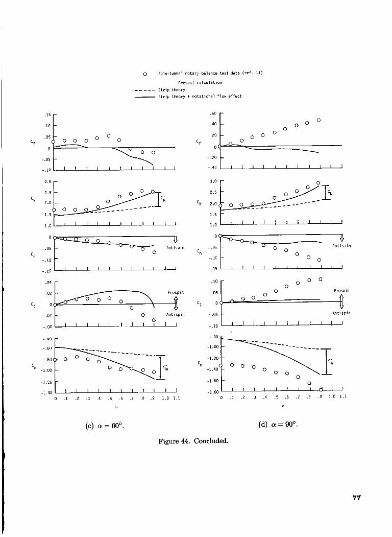
0 Spin-tunnel r o t a r y balance t e s t data ( r e f . 11)
Present c a l c u l a t i o n
----- S t r i p theory - S t r i p theory t r o t a t i o n a l f low e f f e c t
-.05 C"
.10
.15 F
U - Ant ispin -0
0 0 -.05
CY
-.05
-.in I I I I I I I I I 1 1
- Ant is p i n
3.0 r
.60 r
.20 0
CY . 4 0 ~ 0
- ' 20 -.40 5 2.5
'N 2.0 __-- 1.5
-.lo
-.15 I I I I I I I I I I I
.04 r Prospin
0 \
- .40
- .6O
- .80
0 cm -1.00
-1.20
-1.40 1 1 1 1 1 1 1 1 ~ ~ ~ 0 .1 .2 . 3 .4 .5 .6 .7 .8 .9 1.0 1.1
w
A n t i spin
'n
Prospin .05
-1.80 I I I I I 1 1 1 . 3 1 1
0 .1 . 2 . 3 .4 . 5 .6 .7 .8 .9 1.0 1.1 w
(c) a = 60°.
Figure 44. Concluded.
(d) a = W 0
77
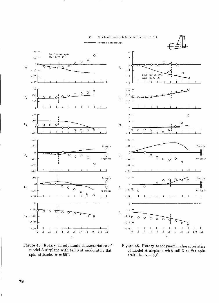
Present c a l c u l a t i o n
.20
.IO
0
- . lo
-.20
-.30
CY
, 0 Spin- tunnel r o t a r y ba lance t e s t data ( r e f . 11)
I-
E q u i l i b r i u m s p i n O mode ( r e f . 14) I 0
- 0 + - -
I l l l l l l l l l )
-.02
.lo r I
I 0 -
.01 1 P r o s p i n
A n t i s p i n 'n
-.01
1
A n t i s p i n Cl
-.05 -
0 I
c, -1.00 -.50 pq-Eaa%o -1.50
-2.00 0 . I .2 . 3 . 4 .5 .6 .7 .8 .9 1.0 1.1
Figure 45. Rotary aerodynamic characteristics of model A airplane with tail 3 at moderately flat spin attitude. (Y = 50'.
'2 . I c - . l
- .2 mode ( r e f . 14)
t .2 r 0
.1 c .n2 r
-.02
-.03 I I I I I 1 I I O I 1
. O : p 0 ; O P r o f i n
-.02 A n t i s p i n
0
-.5 1
0 . I .2 . 3 .4 .5 .6 .7 .8 .9 1.0 1 .1
w
Figure 46. Rotary aerodynamic characteristics of model A airplane with tail 3 ai flat spin attitude. (Y = 80'.
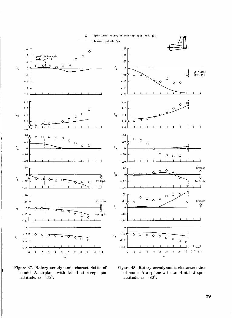
0 Spin-tunnel r o t a r y balance t e s t data ( r e f . 11)
Present c a l c u l a t i o n
"
. 1
CY
CN
C A
'n
C 1
'm
0
- E q u i l i b r i u m spin 0 mode ( r e f . 14) 0
- I
-.l
- . 2
- .3
- . 4
1:: 1 2.0
-
- -
1 1 1 1 1 1 1 1 1 1 l
0 0
0
-.ln t - . 2 0 1 I I l l I I I I I I I
.02 r 0 u
-.02 o u 0 0 A n t i s p i n
.10 II Prospin
- . l o A n t i s p i n
-.20 0
0 I I
0 , 1 . 2 . 3 .4 . 5 .6 .7 .8 .9 1 . 0 1 . 1
w
Figure 47. Rotary aerodynamic characteristics of model A airplane with tail 4 at steep spin attitude. Q = 35'.
CY
.05
-.05
-. 111 0 0 0
-.15 -
-.zn I l l I I I I I 1
.20 r
. l o b 0 0
- . l o t
'm
0 0 -2.0
- 3 . O L l 1 1 I I I I 1 1 0 .1 . 2 . 3 . 4 . 5 . 6 .7 .8 .9 1 . 0 1 . 1
w
Figure 48. Rotary aerodynamic characteristics of model A airplane with tail 4 at flat spin attitude. Q = 80'.
79
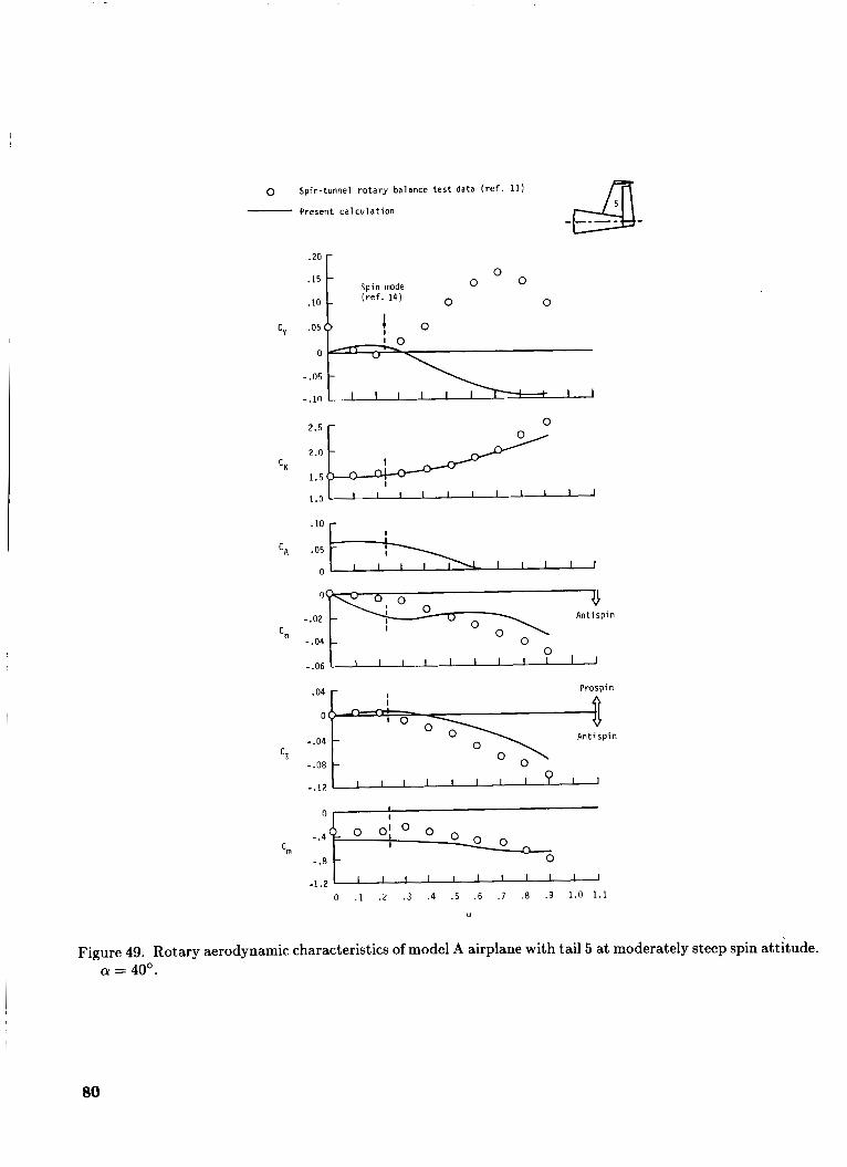
0 Spin-tunnel rotary balance test data (ref. 11)
- Present calculation
.I5
. l 0
Cy . 0 5 0
.20 r 0
0 0
- 0 0 Spin mode (ref. 14) -
t o
.10
c~ .05
0
- I ’
I I I I I
Anti s p i n -.02 0
-.04 O n ‘n
Cl
Prospin
-.04
-.08
-.1?
n , I
-1.2 0 . I . 2 .3 .4 . 5 .6 .7 .8 .9 1.0 1.1
Figure 49. Rotary aerodynamic characteristics of model A airplane with tail 5 at moderately steep spin attitude. a = 40’.
80
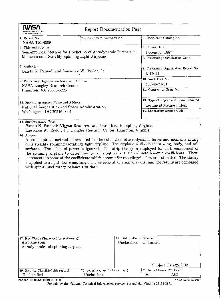
Nalinnal Aeronautcs and
L. Report No. 2. Government Accession No. NASA TM-4009
Report Documentation Page
3. Recipient’s Catalog No.
3. Performing Organization Name and Address NASA Langley Research Center Hampton, VA 23665-5225
L2. Sponsoring Agency Name and Address National Aeronautics and Space Administration Washington, DC 20546-0001
5. Report Date Semiempirical Method for Prediction of Aerodynamic Forces and Moments on a Steadily Spinning Light Airplane
December 1987 I------ 6. Performing Organization Code
&. Title and Subtitle
10. Work Unit No.
506-46-21-01 11. Contract or Grant No.
13. Type of Report and Period Covered
Technical Memorandum 14. Sponsoring Agency Code
7. Author(s) Bandu N. Pamadi and Lawrence W. Taylor, Jr.
.9. Security Classif.(of this report) 20. Security Classif.(of this page) 21. No. of Pages Unclassified Unclassified 86
8. Performing Organization Report No.
L-15654
22. Price A05
Lawrence W. Taylor, Jr.: Langley Research Center, Hampton, Virginia. L6. Abstract
A semiempirical method is presented for the estimation of aerodynamic forces and moments acting on a steadily spinning (rotating) light airplane. The airplane is divided into wing, body, and tail surfaces. The strip theory is employed for each component of the spinning airplane to determine its contribution to the total aerodynamic coefficients. Then, increments to some of the coefficients which account for centrifugal effect are estimated. The theory is applied to a light, low-wing, single-engine general aviation airplane, and the results are compared with spin-tunnel rotary balance test data.
The effect of power is ignored.
Airplane spin Unc1assific.d-Unlimited Aerodynamics of spinning airplane