SEMIDEFINITE PROGRAMMING RELAXATIONS FORTHE QUADRATIC ASSIGNMENT PROBLEM�Qing Zhaox Stefan E. Karischy, Franz Rendlz, Henry Wolkowiczx,March 1997University of Waterloo University of CopenhagenCORR Report 95-27 DIKU TR-96/32AbstractSemide�nite programming (SDP) relaxations for the quadratic assignment problem (QAP)are derived using the dual of the (homogenized) Lagrangian dual of appropriate equivalentrepresentations of QAP. These relaxations result in the interesting, special, case where onlythe dual problem of the SDP relaxation has strict interior, i.e. the Slater constraint quali�-cation always fails for the primal problem. Although there is no duality gap in theory, thisindicates that the relaxation cannot be solved in a numerically stable way. By exploring thegeometrical structure of the relaxation, we are able to �nd projected SDP relaxations. Thesenew relaxations, and their duals, satisfy the Slater constraint quali�cation, and so can besolved numerically using primal-dual interior-point methods.For one of our models, a preconditioned conjugate gradient method is used for solving thelarge linear systems which arise when �nding the Newton direction. The preconditioner isfound by exploiting the special structure of the relaxation. See e.g. [41] for a similar approachfor solving SDP problems arised from the control applications.Numerical results are presented which indicate that the described methods yield at leastcompetitive lower bounds.Contents1 INTRODUCTION 21.1 The Quadratic Assignment Problem . . . . . . . . . . . . . . . . . . . . . . . . . 21.2 Semide�nite Programming . . . . . . . . . . . . . . . . . . . . . . . . . . . . . . . 31.3 Goals . . . . . . . . . . . . . . . . . . . . . . . . . . . . . . . . . . . . . . . . . . 31.4 Main Results . . . . . . . . . . . . . . . . . . . . . . . . . . . . . . . . . . . . . . 41.5 Outline . . . . . . . . . . . . . . . . . . . . . . . . . . . . . . . . . . . . . . . . . 41.6 Preliminaries . . . . . . . . . . . . . . . . . . . . . . . . . . . . . . . . . . . . . . 4�Revised version. To appear in Journal of Combinatorial Optimization. This report is available by anonymousftp or over WWW at ftp://orion.uwaterloo.ca/pub/henry/reports/ABSTRACTS.htmlyUniversity of Copenhagen, Department of Computer Science, Universitetsparken 1, DK-2100 Copenhagen,DenmarkzGraz University of Technology, Department of Mathematics, Steyrergasse 30, A-8010 Graz, AustriaxUniversity of Waterloo, Department of Combinatorics and Optimization, Faculty of Mathematics, Waterloo,Ontario, N2L 3G1 Canada

2 SDP and LAGRANGIAN RELAXATION 52.1 The Direct Approach to SDP Relaxation . . . . . . . . . . . . . . . . . . . . . . . 62.2 Lagrangian Relaxation . . . . . . . . . . . . . . . . . . . . . . . . . . . . . . . . . 73 GEOMETRY of the RELAXATION 103.1 The Minimal Face . . . . . . . . . . . . . . . . . . . . . . . . . . . . . . . . . . . 113.2 The Projected SDP Relaxation . . . . . . . . . . . . . . . . . . . . . . . . . . . . 154 TIGHTENING THE RELAXATION 164.1 The Gangster Operator . . . . . . . . . . . . . . . . . . . . . . . . . . . . . . . . 164.2 The Gangster Operator and Redundant Constraints . . . . . . . . . . . . . . . . 184.3 Inequality Constraints . . . . . . . . . . . . . . . . . . . . . . . . . . . . . . . . . 214.4 A Comparison with Linear Relaxations . . . . . . . . . . . . . . . . . . . . . . . . 215 PRIMAL-DUAL INTERIOR-POINT ALGORITHM 225.1 Generic SDP Model . . . . . . . . . . . . . . . . . . . . . . . . . . . . . . . . . . 225.2 Application to the Gangster Model . . . . . . . . . . . . . . . . . . . . . . . . . . 245.2.1 The Preconditioned Conjugate Gradient Method . . . . . . . . . . . . . . 245.2.2 Stopping Criterion for the Interior-Point Method . . . . . . . . . . . . . . 255.3 Application to the Block Model . . . . . . . . . . . . . . . . . . . . . . . . . . . . 265.3.1 Predictor Corrector Approach . . . . . . . . . . . . . . . . . . . . . . . . . 275.3.2 A Cutting Plane Approach . . . . . . . . . . . . . . . . . . . . . . . . . . 275.4 Strictly Feasible Points for Both Models . . . . . . . . . . . . . . . . . . . . . . . 286 NUMERICAL RESULTS 29A Notation 351 INTRODUCTIONSemide�nite programming (SDP) has proven to be very successful in providing tight relaxationsfor hard combinatorial problems, such as the max-cut problem. The quadratic assignment prob-lem (QAP) is a well known NP -hard combinatorial problem where problems of dimension n = 16can be considered large. We study SDP relaxations for QAP. In the process we handle severalinteresting complications that arise, e.g. no constraint quali�cation for the SDP relaxation andloss of sparsity when solving for the search direction.1.1 The Quadratic Assignment ProblemThe QAP in the trace formulation is(QAP ) �� := minX2� traceAXBXT � 2CXT ;where A;B are real symmetric n� n matrices, C is a real n� n matrix, and � denotes the setof permutation matrices. (We assume n � 4 to avoid trivialities.) QAP is used to model the2

problem of allocating a set of n facilities to a set of n locations while minimizing the quadraticobjective arising from the distance between the locations in combination with the ow betweenthe facilities. The QAP is well known to be NP -hard [39] and, in practice, problems of moderatesizes, such as n = 16, are still considered very hard. For recent surveys on QAP, see thearticles Burkard [6], and Rendl, Pardalos, Wolkowicz [30]. An annotated bibliography is givenby Burkard and C�ela [7].The QAP is a classic problem that still de�es all approaches for its solution and whereproblems of dimension n � 16 can be considered large scale. A \Nugent type" test problem ofdimension n = 22 (based on the problems introduced in [29] and obtainable from QAPLIB [8])has only recently been solved to optimality by Br�ungger et al. [1] using high power computingfacilities and the classical Gilmore-Lalwer bound (GLB) [13, 26]. The failure to solve largerproblems using branch and bound techniques is due mainly to the lack of bounds which aretight and at the same time cheap to compute. Even though GLB is cheap to compute, it is ingeneral not very tight. For solving the Nugent type problem of dimension n = 22; more than 48billion (!) subproblems had to be solved (see [1]).Stronger bounds based on linear programming relaxations are used by Adams and Johnson[2], and by Resende, Ramakrishnan and Drezner [37]. These are quite expensive to compute andcan only be applied to problems of dimension n � 30. The latter bounds have been applied inbranch and bound for instances of dimension n � 15, see Ramakrishnan, Resende and Pardalos[34]. More recently, Rijal [38], and J�unger and Kaibel [21] studied the QAP polytope and foundtighter linear relaxations of QAP.Another class of lower bounds is the class of eigenvalue bounds which are based on orthogonalrelaxations, see e.g. [12, 16, 36, 23]. Even though they are stronger for many (symmetric)problems of dimension n � 20 and are of reasonable computational cost for all instances inQAPLIB, they are not very well suited for application in branch and bound methods, sincetheir quality deteriorates in lower levels of the branching tree, see Clausen et al. [10].1.2 Semide�nite ProgrammingSemide�nite programming is an extension of linear programming where the nonnegativity con-straints are replaced by positive semide�niteness constraints on matrix variables. SDP has beenshown to be a very powerful tool in several di�erent areas, e.g. positive de�nite completionproblems, maximum entropy estimation, and bounds for hard combinatorial problems, see e.g.the survey of Vandenberghe and Boyd [42].Though SDP has been studied in the past, as part of the more general cone programmingproblem, see e.g. [11, 43], there has been a renewed interest due to the successful applicationsto discrete optimization [27, 14] and to systems theory [5]. In addition, the relaxations areequivalent to the reformulation and linearization technique, see e.g. the survey discussion in[40], which provides further evidence of successful applications.1.3 GoalsIn this paper we test the e�cacy of using semide�nite programming to provide strong relaxationsfor QAP. We try to address the following questions:3

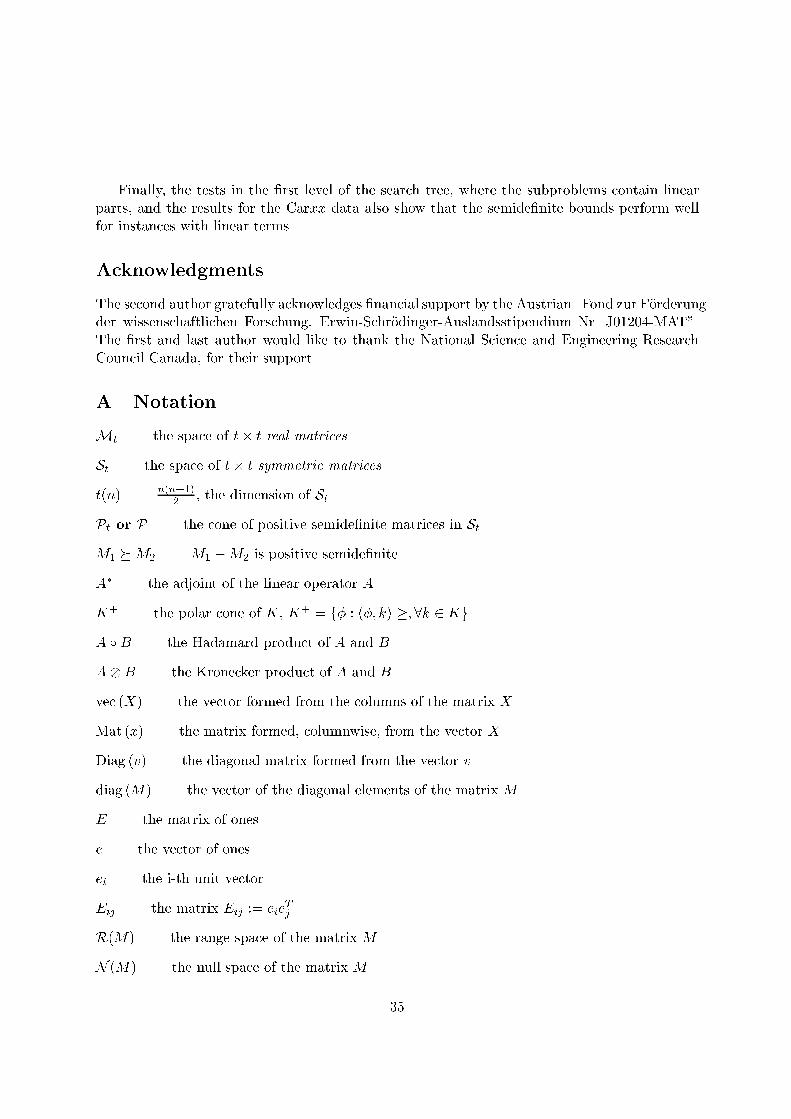
1. How to overcome many interesting numerical and theoretical di�culties, e.g. loss of con-straint quali�cation and loss of sparsity in the optimality conditions?2. Can the new bound compete with other bounding techniques in speed and quality?3. Can we improve the bounds or solve existing tough instances of QAP, e.g. the Nugent testproblems?4. Can we improve the bound further by adding new facet inequalities?1.4 Main ResultsMotivated by the numerical and theoretical success of SDP for e.g. the max-cut problem [17,19, 14, 15], we study SDP relaxations for QAP. These relaxations also prove to be numericallysuccessful. In addition, the relaxation of the linear equality constraints, corresponding to thedoubly stochastic property of permutation matrices, implies that the SDP relaxation does notsatisfy the Slater constraint quali�cation. Although there is no duality gap in theory, sincethe dual does satisfy Slater's constraint quali�cation, this leads to an unbounded dual optimalsolution set. Numerical di�culties can arise when trying to implement interior-point methods,see Example 3.1 below. However, the minimal face of the semide�nite cone can be found usingthe structure of the barycenter of the convex hull of the permutation matrices. In fact, theminimal face is completely de�ned by the row and column sum property of permutation matrices.Surprisingly, the 0,1 property does not change the minimal face. Then, the primal problem canbe projected onto the minimal face. This yields a regularized SDP of smaller dimension.The special structure of the minimal face can be exploited to �nd an inexpensive precon-ditioner. This enables us to solve the large linear system arising from the Newton equation ininterior-point methods.We also present numerical results which indicate that this new approach yields at leastcompetitive bounds.1.5 OutlineWe complete this section with basic notation and some preliminary results. (We include anappendix with a list of notation at the end of the paper.) In Section 2 we derive the SDPrelaxations. We initially use the dual of the homogenized Lagrangian dual to get a preliminaryrelaxation. In Section 3 we study the geometry of the semide�nite relaxation and show howto project onto the minimal face of the relaxation. This guarantees that Slater's constraintquali�cation holds. This yields a basic semide�nite relaxation which is then tightened by addingadditional constraints (in Section 4). We describe practical aspects of applying a primal-dualinterior-point method in Section 5. We conclude with our numerical results in Section 6.1.6 PreliminariesWe work with the space of t � t real matrices denoted Mt, and the space of t � t symmetricmatrices denoted St. Diag (v) denotes the diagonal matrix formed from the vector v and con-versely, (the adjoint of Diag (v)) diag (M) is the vector of the diagonal elements of the matrix4

M ; R(M), N (M) denote the range space and null space, respectively; e is the vector of onesand ei is the i-th unit vector; E denotes the matrix of ones and Eij := eieTj ; M:;t:j refers tothe columns t to j of M and Mi:s;: refers to the rows i to s of M: The set of matrices withrow and column sums one, is denoted by E := fX : Xe = XT e = eg and is called the set ofassignment constraints; the set of (0,1)-matrices is denoted by Z := fX : Xij 2 f0; 1gg; the setof nonnegative matrices is denoted by N := fX : Xij � 0g; while the set of orthogonal matricesis denoted by O := fX : XXT = XTX = Ig; where I is the identity matrix.For symmetric matrices M1 � M2 (M1 � M2) refers to the L�owner partial order, i.e. thatM1 �M2 is negative semide�nite (negative de�nite, respectively); similar de�nitions hold forpositive semide�nite and positive de�nite; V � W; (V < W ) refers to elementwise orderingof the matrices. The space of symmetric matrices is considered with the trace inner product< M;N >= traceMN:We use the Kronecker product, or tensor product, of two matrices, A B, when discussingthe quadratic assignment problem QAP; vec (X) denotes the vector formed from the columns ofthe matrix X, while Mat (x) denotes the matrix formed from the vector x. Note that, see e.g.[20],1. (AB)(U V ) = AU BV:2. vec (AY B) = (BT A)vec (Y ):3. (AB)T = AT BT :The Hadamard product or elementwise product of two matrices A and B is denoted A � B:We partition a symmetric matrix Y 2 Sn2+1 into blocks as follows.Y = " y00 Y T0Y0 Z # = 266664 y00 Y 01 : : : Y 0nY 10 Y 11 : : : Y 1n... ... . . . ...Y n0 Y n1 : : : Y nn 377775 ; (1.1)where we use the index 0 for the �rst row and column. Hence Y0 2 <n2 , Z 2 Sn2 , Y p0 2 <n, andY pq 2 Mn. When referring to entry r; s 2 f1; 2; : : : ; n2g of Z, we also use the pairs (i; j); (k; l)with i; j; k; l 2 f1; 2; : : : ; ng. This identi�es the element in row r = (i � 1)n + j and columns = (k � 1)n + l by Y(i;j);(k;l). This notation is going to simplify both the modeling and thepresentation of properties of the relaxations. If we consider Z as a matrix consisting of n � nblocks Y ik, then Y(i;j);(k;l) is just element (j; l) of block (i; k).2 SDP and LAGRANGIAN RELAXATIONIn this section we present a \�rst" SDP relaxation for QAP. This comes from \lifting" theproblem into a higher dimensional space of symmetric matrices. The QAP is a quadratic (0; 1)-problem with additional constraints prescribed by the permuation matrices X 2 �, which canalso be represented by binary vectors vec (X). The embedding in Sn2+1 is obtained by 1vec (X) ! (1; vec (X)T );5

which is due to its construction as diadic product a symmetric and positive semide�nite matrix.However, it is interesting and useful to know that the relaxation comes from the dual of the(homogenized) Lagrangian dual. Thus SDP relaxation is equivalent to Lagrangian relaxationfor an appropriately constrained problem. (See also [32].) In the process we see several of theinteresting operators that arise in the relaxation. The structure of this SDP relaxation is thenused to �nd the projected relaxation which is the actual one we use for our bounds. As in [32],we see that adding, possibly redundant, quadratic constraints often tightens the SDP relaxationobtained through the Lagrangian dual.It is well known that the set of permutation matrices � can be characterized as the inter-section of (0,1)-matrices with E and O, i.e.� = E \ Z = O \ Z; (2.1)see e.g. [16]. Therefore, we can rewrite QAP as(QAPE ) �� := min traceAXBXT � 2CXTs.t. XXT = XTX = IXe = XT e = eX2ij �Xij = 0; 8i; j:We can see that there are a lot of redundant constraints in (QAPE ). However, as we show below,they are not necessarily redundant in the SDP relaxations.Additional redundant (but useful in the relaxation) constraints will be added below, e.g. wecan use the fact that the rank-one matrices formed from the columns of X, i.e. X:iXT:j ; arediagonal matrices if i = j; while their diagonals are 0 if i 6= j:2.1 The Direct Approach to SDP RelaxationWe �rst show how the SDP relaxation can be obtained directly from QAP. This involves liftingthe vector x = vec (X) into the matrix space Sn2+1:We now outline this for the quadratic constraints that arise from the fact that X is a (0; 1),orthogonal matrix . Let X 2 �n be a permutation matrix and, again, let x = vec (X) andc = vec (C): Then the objective function for QAP isq(X) = traceAXBXT � 2CXT= xT (B A)x� 2cTx= trace xxT (B A)� 2cTx= traceLQYX ;where we de�ne the (n2 + 1)� (n2 + 1) matricesLQ := " 0 �vec (C)T�vec (C) B A # ; (2.2)and YX := " x0 xTx xxT # : (2.3)6

This shows how the objective function of QAP is transformed into a linear function in the SDPrelaxation; where we have added the constraint (YX)00 = 1: Note that if we denote Y = YX ,then the element Y(i;j);(k;l) corresponds to xijxkl.We already have three constraints on the matrix Y , i.e. it is positive semide�nite, the top-leftcomponent y00 = 1, and it is rank-one. The �rst two constraints are tractable constraints; whilethe rank-one constraint is too hard to satisfy and is discarded in the SDP relaxation.In order to guarantee that the matrix Y , in the case that it is rank one, arises from apermutation matrixX, we need to add additional constraints. For example, the (0,1)-constraintsX2ij � x0Xij = 0 are equivalent to the restriction that the diagonal of Y is equal to its �rst row(or column). This results in the arrow constraint, see (2.15) below. Similarly, the orthogonalityconstraint, XXT = I can be written asXXT = nXk=1X:kXT:k = I:Each rank-one matrix in the sum is a diagonal n� n block of Y , i.e. we get the block diagonalconstraint, see (2.16). Similarly, the orthogonality constraint written as XTX = I results in theblock o� diagonal constraints, see (2.17). The SDP relaxation with these constraints, as well asthe ones arising from the row and column sums equal 1, is given below in (2.14). Also, we willsee below that the SDP relaxation is exact if we do not relax the rank-one constraint on Y . (SeeTheorem 2.1.)2.2 Lagrangian RelaxationIn this section we will investigate the relaxation of the constraints in (QAPE ) via Lagrangianduality. We show that the dual of the Lagrangian dual results in an SDP relaxation. Also, thereis no duality gap between the Lagrangian relaxation and its dual, so solving the SDP relaxationis equivalent to solving the Lagrangian relaxation. Though SDP relaxations can be obtainedmore simply in a direct fashion, once the form of the relaxation is known, it is important to knowwhere the relaxation comes from in order to recover good approximate feasible solutions. Moreprecisely, we can use the optimal solution of the dual of the SDP in the Lagrangian relaxation of(QAPE ) and then �nd the optimal matrix X where this Lagrangian attains its minimum. ThisX is then a good approximation for the original QAP, see [25].After changing the row and column sum constraints into kXe � ek2 + kXT e � ek2 = 0 weconsider the following equivalent problem to QAP.(QAPO) �O := min traceAXBXT � 2CXTs.t. XXT = IXTX = IkXe� ek2 + kXT e� ek2 = 0X2ij �Xij = 0; 8i; j:We �rst add the (0,1) and row-column sum constraints to the objective function using Lagrangemultipliers Wij and u0 respectively.�O = minXXT=XTX=ImaxW;u0 ftraceAXBXT � 2CXT +PijWij(X2ij �Xij)+ u0(kXe� ek2 + kXT e� ek2)g: (2.4)7

Interchanging min and max yields�O � �L := maxW;u0 minXXT=XTX=I ftraceAXBXT � 2CXT +PijWij(X2ij �Xij)+ u0(kXe � ek2 + kXT e� ek2)g: (2.5)We now continue with the relaxation and homogenize the objective function by multiplying bya constrained scalar x0 and increasing the dimension of the problem by 1. We homogenize theproblem since that simpli�es the transition to a semide�nite programming problem.�O � �L = maxW minXXT=XTX=I;x20=1 ftrace [AXBXT +W (X �X)T+ u0(kXek2 + kXT ek2)� x0(2C +W )XT ]� 2x0u0eT (X +XT )e+ 2nu0g: (2.6)Introducing a Lagrange multiplier w0 for the constraint on x0 and Lagrange multipliers Sb forXXT = I and So for XTX = I we get the lower bound �R�O � �L � �R := maxW;Sb;So;u0;w0 minX; x0 ftrace [AXBXT + u0(kXek2 + kXT ek2)+W (X �X)T + w0x20 + SbXXT + SoXTX]� trace x0(2C +W )XT � 2x0u0eT (X +XT )e� w0 � trace Sb � traceSo + 2nu0g: (2.7)Both inequalities can be strict, i.e. there can be duality gaps in each of the Lagrangian relax-ations. Following is an example of a duality gap that arises from the Lagrangian relaxation ofthe orthogonality constraint.Example 2.1 Consider the the pure quadratic, orthogonally constrained problem�� := min traceAXBXTs.t. XXT = I; (2.8)with 2� 2 matrices A = 1 00 2 ! ; B = 3 00 4 ! :The dual problem is �D := max �traceSs.t. (B A+ I S) � 0S = ST : (2.9)Then �� = 10: But is the dual optimal value �D also 10? We haveB A = 0BBB@ 3 0 0 00 6 0 00 0 4 00 0 0 8 1CCCA :Then in order to satisfy dual feasibility, we must have S11 � �3 and S22 � �6. In order tomaximize the dual, equality must hold. Therefore �traceS = 9 in the optimum. Thus we haveduality gap for this simple example. 8

In (2.7), we grouped the quadratic, linear, and constant terms together. We now de�ne x :=vec (X), yT := (x0; xT ) and wT := (w0; vec (W )T ) and get�R = maxw;Sb;So;u0 miny fyT �LQ +Arrow (w) + B0Diag (Sb) + O0Diag (So) + u0D� y� w0 � trace Sb � traceSog; (2.10)where LQ is as above and the linear operatorsArrow (w) := " w0 �12wT1:n2�12w1:n2 Diag (w1:n2) # ; (2.11)B0Diag (S) := " 0 00 I Sb # ; (2.12)O0Diag (S) := " 0 00 So I # ; (2.13)and D := " n �eT eT�e e I E #+ " n �eT eT�e e E I # :There is a hidden semide�nite constraint in (2.10), i.e. the inner minimization problem isbounded below only if the Hessian of the quadratic form is positive semide�nite. In this casethe quadratic form has minimum value 0. This yields the following SDP.(DO) max �w0 � trace Sb � traceSos.t. LQ +Arrow (w) + B0Diag (Sb) + O0Diag (So) + u0D � 0:We now obtain our desired SDP relaxation of (QAPO) as the Lagrangian dual of (DO): Weintroduce the (n2 + 1) � (n2 + 1) dual matrix variable Y � 0 and derive the dual program tothe SDP (DO): (SDPO) min traceLQYs.t. b0diag (Y ) = I; o0diag (Y ) = Iarrow (Y ) = e0; traceDY = 0Y � 0; (2.14)where the arrow operator, acting on the (n2+1)� (n2+1) matrix Y , is the adjoint operator toArrow (�) and is de�ned by arrow (Y ) := diag (Y )� (0; (Y0;1:n2)T ; (2.15)i.e. the arrow constraint guarantees that the diagonal and 0-th row (or column) are identical.The block-0-diagonal operator and o�-0-diagonal operator acting on Y are de�ned byb0diag (Y ) := nXk=1Y(k;�);(k;�) (2.16)9

and o0diag (Y ) := nXk=1Y(�;k);(�;k): (2.17)These are the adjoint operators of B0Diag (�) and O0Diag (�), respectively. The block-0-diagonaloperator guarantees that the sum of the diagonal blocks equals the identity. The o�-0-diagonaloperator guarantees that the trace of each diagonal block is 1, while the trace of the o�-diagonalblocks is 0. These constraints come from the orthogonality constraints, XXT = I andXTX = I;respectively.We have expressed the orthogonality constraints with both XXT = I and XTX = I. It isinteresting to note that this redundancy adds extra constraints into the relaxation which arenot redundant. These constraints reduce the size of the feasible set and so tighten the bounds.Proposition 2.1 Suppose that Y is feasible for the SDP relaxation (2.14). Then Y is singular.Proof. Note that D 6= 0 is positive semide�nite. Therefore Y has to be singular in order tosatisfy the constraint traceDY = 0. 2This means that the feasible set of the primal problem (SDPO) has no interior. It is notdi�cult to �nd an interior-point for the dual (DO), which means that Slater's constraint quali-�cation (strict feasibility) holds for (DO). Therefore (SDPO) is attained and there is no dualitygap in theory, for the usual primal-dual pair. However, if Slater's constraint quali�cation fails,then this is not the proper dual, since perturbations in the right-hand-side will not result in thedual value. This is because we cannot stay exactly feasible in the dual, � 0, since the interior isempty, see [35]. In fact we may never attain the supremum of (DO), which may cause instabilitywhen implementing any kind of interior-point method. Since Slater's constraint quali�cationfails for the primal, the set of optimal solutions of the dual is an unbounded set, and an interior-point method may never converge. Therefore we have to express the feasible set of (SDPO) insome lower dimensional space. We study this below when we project the problem onto a face ofthe semide�nite cone.However, if we add the rank-one condition, then the relaxation is exact.Theorem 2.1 Suppose that Y is restricted to be rank-one in (SDPO), i.e. Y = 1x ! (1 xT ),for some x 2 <n2 . Then the optimal solution of (SDPO) provides the permutation matrixX = Mat (x) that solves the QAP.Proof. The arrow-constraint in (SDPO) guarantees that the diagonal of Y is 0 or 1. The0-diagonal and assignment constraint now guarantee that Mat (x) is a permutation matrix.Therefore the optimization is over the permutation matrices and so the optimum of QAP isobtained. 23 GEOMETRY of the RELAXATIONWe de�ne FO to be the feasible set of the semide�nite relaxation (SDPO). There are twodi�culties regarding our feasible set FO. It is easy to see that there are redundant constraints10

in (SDPO). The other di�culty is that FO has no positive de�nite feasible point. Hence, theoptimal set of the dual is unbounded and we cannot apply an (feasible or infeasible) interior-pointmethod directly. In fact, the dual can be unattained.Example 3.1 Consider the SDP pair(P ) min 2X12s.t. diag (X) = 01 !X � 0 (D) max y2s.t. " y1 00 y2 # � " 0 11 0 #Slater's condition holds for the dual but not for the primal. The optimal value for both is 0. Theprimal is attained, but the dual is not.3.1 The Minimal FaceIn order to overcome the above di�culties, we need to explore the geometrical structure of FO.It is easy to see that YX := 1vec (X) ! (1 vec (X)T ); X 2 �are feasible points of FO. Moreover, these points are rank-one matrices and are, therefore,contained in the set of extreme points of FO, see e.g. Pataki [31]. We need only consider faces ofFO which contain all of these extreme points. Therefore we are only interested in the minimalface, which is the intersection of all these faces.We need to take a closer look at the assignment (row and column sums) constraints de�nedby E .Surprisingly, it is only these constraints that are needed to de�ne the minimal face. (This isnot true in general, see Example 3.2 below.) Alternatively, we can describe these constraints asfollows. With x = vec (X), the constraints areXT e = e() 26664 eT 0 � � � � � � 00 eT 0 � � � 0� � � � � � � � � � � � � � �0 � � � � � � 0 eT 37775 x = eand Xe = e() h I I � � � � � � I ix = e:Thus, the assignment constraints are equivalent toTx = e;where T := " I eTeT I # : (3.1)11

We now multiply with xT from the right and use the fact that x is a binary vector. We getTxxT = e(diag (xxT ))T ;and also Tdiag (xxT ) = e:These two conditions are equivalent to T YX = 0; (3.2)where T := [�ejT ]; and (3.2) now corresponds to the embedding of the assignment constraintsinto Sn2+1.Before we characterize the minimal face of FO we de�ne the following (n2+1)�((n�1)2+1)matrix. V := " 1 01n(e e) V V # ; (3.3)where V is an n � (n � 1) matrix containing a basis of the orthogonal complement of e, i.e.V T e = 0. Our choice for V is V := " In�1�eTn�1 # :In fact, V is a basis of the null space of T , i.e. T V = 0.The following theorem characterizes the minimal face by �nding the barycenter of the convexhull of the permutation matrices. The barycenter has a very simple and elegant structure.Theorem 3.1 De�ne the barycenter Y := 1n! XX2�n YX : (3.4)Then:1. Y has a 1 in the (0,0) position and n diagonal n � n blocks with diagonal elements 1=n:The �rst row and column equal the diagonal. The rest of the matrix is made up of n� nblocks with all elements equal to 1=(n(n � 1)) except for the diagonal elements which are0. Y = 264 1 1neT1ne h 1n2E Ei+ h 1n2(n�1) (nI �E) (nI �E)i 375 :2. The rank of Y is given by rank (Y ) = (n� 1)2 + 1:3. The n2 + 1 eigenvalues of Y are given in the vector(2; 1n� 1eT(n�1)2 ; 0eT2n�1)T :12

4. The null space and range space areN (Y ) = R(T T ) and R(Y ) = R(V ) (so that N (T ) = R(V ) ):Proof. Fix X 2 � and letY = YX = 1vec (X) ! (1 vec (X)T ):We now proceed to �nd the structure of Y : Consider the entries of the 0th row of Y . SinceY0;(i�1)n+j = 1 means i is assigned to j; there are (n� 1)! such permutations. We conclude thatthe components of the 0 row (and column) of Y are given byY0;(i�1)n+j = 1n! (n� 1)! = 1n:Now consider the entries of Y in the other rows, denoted Y(p;q);(i;j).i) If p = i and q = j, then Y(p;q);(i;j) = 1 means that i is assigned to j and there are (n� 1)!such permutations. Therefore the diagonal elements areY(i;j);(i;j) = 1n! (n� 1)! = 1n:ii) Now suppose that p 6= i and q 6= j, i.e. the element is an o�-diagonal element in ano�-diagonal block. Then Y(p;q);(i;j) = 1 means that i is assigned to j and p is assigned toq: Since there are (n� 2)! such permutations, we get thatY(p;q);(i;j) = 1n! (n� 2)! = 1n(n� 1) :iii) Otherwise, suppose that p = i or q = j, but not both, i.e. we consider the o�-diagonalelements of the diagonal blocks and the diagonal elements of the o�-diagonal blocks. By theproperty of permutation matrices, these elements must all be 0, i.e. they correspond to theo�-diagonal elements of X:j �XT:j and the diagonal elements of elements of X:q �XT:j ; q 6= j.This proves the representation of Y in 1.Let us �nd the rank and eigenvalues of Y . We partitionY = " 1 1neT1ne Z # ;thus de�ning the block Z. We have" 1 01ne I # Y " 1 1neT0 I # = " 1 00 S # ; (3.5)13

where S = Z � 1n2E. As a result, we haverank (Y ) = 1 + rank (S):From the structure of Y , we see thatS = 1n2(n� 1)(nIn�1 �E) (nIn�1 �E):The eigenvalues of nIn�1 � E are n (with multiplicity n � 1) and 0. By the fact that theeigenvalues of a Kronecker product are found from the Kronecker product of eigenvalues, wehave that the eigenvalues of S are 1=(n� 1) (with multiplicity (n� 1)2) and 0 (with multiplicity2n� 1). Therefore, we haverank (Y ) = 1 + rank (S) = (n� 1)2 + 1:This proves 2.By (3.5) and the rank, we see that the eigenvalues of Y are 1=(n � 1) (with multiplicity(n� 1)2) and 2 and 0 (with multiplicity 2n� 1). This proves 3.Note that u 2 N (S), � 1neTuu ! 2 N (Y ): (3.6)It is well known that rank (T ) = 2n� 1 and we can verify that ST T = 0. So we haveN (Y ) = ( � 1neTuu ! : u 2 R(T T )) :In addition, we can now verify thatV T � 1neTuu ! = 0 for u 2 R(T T ):This proves 4. 2With the above characterization of the barycenter, we can �nd the minimal face of P thatcontains the feasible set of the relaxation SDP. We let t(n) := n(n+1)2 .Corollary 3.1 The dimension of the minimal face is t((n � 1)2 + 1). Moreover, the minimalface can be expressed as V S(n�1)2+1V T .The above characterization of the barycenter yields a characterization of the minimal face.At �rst glance it appears that there would be a simpler proof for this characterization, the proofwould use only the row and column sums constraints. Finding the barycenter is the key inexploiting the geometrical structure of a given problem with an assignment structure. However,it is not always true that the other constraints in the relaxation are redundant, as the followingshows. 14

Example 3.2 Consider the constraintsx1 = 1x1 +x2 +x3 +x4 = 1x1; x2; x3; x4 � 0The only solution is (1; 0; 0; 0). Hence the barycenter of the relaxation is the set with only arank one matrix in it. However, the null space of the above system has dimension 3. Thus theprojection using the null space yields a minimal face with matrices of dimension greater than 1.3.2 The Projected SDP RelaxationIn Theorem 3.1, we presented explicit expressions for the range and null space of the barycenter,denoted Y : It is well known, see e.g. [4], that the faces of the positive semide�nite cone arecharacterized by the nullspace of points in their relative interior, i.e. K is a face ifK = fX � 0 : N (X) � Sg = fX � 0 : R(X) � S?g;and relintK = fX � 0 : N (X) = Sg = fX � 0 : R(X) = S?g;where S is a given subspace. In particular, if X 2 relintK; the matrix V is n� k, and R(V ) =R(X), then K = V PkV T :Therefore, using V in Theorem 3.1, we can project the SDP relaxation (SDPO) onto the minimalface. The projected problem is(QAPR1) �R1 := min trace (V TLQV )Rs.t. b0diag (V RV T ) = I; o0diag (V RV T ) = Iarrow (V RV T ) = e0; R � 0 (3.7)Note that the constraint trace (V TDV )R = 0 can be dropped since it is always satis�ed, i.e.DV = 0. We are going to refer to (QAPR1) as the basic relaxation of QAP.By construction, this program satis�es the generalized Slater constraint quali�cation for bothprimal and dual. Therefore there will be no duality gap, the optimal solutions are attained forboth primal and dual, and both the primal and dual optimal solution sets are bounded.Using the fact that T V = 0, we get the following lemma which gives some interestingproperties of matrices of the form V RV T ; i.e. of matrices in the span of the minimal face.These properties are closely related to the row and column sums equal 1 constraints. We willsee below that these properties cause some of the other constraints to be redundant in the SDPrelaxation.Lemma 3.1 Let R 2 S(n�1)2+1 be arbitrary and letY = V RV T ;where V is given in (3.3). Then, using the block notation of (1.1), we have15

a) y00 = r00, Y 0je = r00, and nPj=1Y 0j = r00eT :b) Y 0j = eTY ij; for i; j = 1; : : : ; n:c) nPi=1 Y ij = eY 0j and nPi=1diag (Y ij) = Y j0; for j = 1; : : : ; n:Proof. We can verify that y00 = r00 from the de�nitions. Using the fact that T V =h �e T i V = 0; we have T Y = T V RV T = 0:The rest of the proof follows from expanding T Y = 0: 2The projection eliminates the constraints T Y = 0. After the projection, one problem re-mains. There are still redundant constraints in the relaxation. This creates unnecessary com-plications when applying interior-point methods, i.e. the linear systems do not necessarily haveunique solutions. But, using Lemma 3.1, we can observe that in the basic relaxation (QAPR1)parts of the block-0-diag and o�-0-diag operators are redundant. This is because the implicitpresence of the assignment constraints in combination with the arrow operator forces y00 = 1.The main diagonal elements of the images of both operators are equal to one automatically.Part b) of Lemma 3.1 relates the row sums of the diagonal blocks to the corresponding parts ofthe 0 column of Y . Therefore the sum of the diagonal blocks has row sums equal to one, whichmakes one additional element per row dependent. The same can be observed for the o�-0-diagoperator. The dimension of the image space of both operators now reduces to (n2 � 3n)=2. Weassume from now on that the operators are de�ned such that they cover only a set of (n2�3n)=2linearly independent equalities.4 TIGHTENING THE RELAXATION4.1 The Gangster OperatorThe feasible set of the SDP relaxation is convex but not polyhedral. It contains the set ofmatrices of the form YX corresponding to the permutation matrices X 2 �: But the SDPrelaxations, discussed above, can contain many points that are not in the a�ne hull of theseYX : In particular, it can contain matrices with nonzeros in positions that are zero in the a�nehull of the YX : We can therefore strengthen the relaxation by adding constraints correspondingto these zeros.Note that the barycenter Y is in the relative interior of the feasible set. Therefore thenull space of Y determines the dimension of the minimal face which contains the feasible set.However, the dimension of the feasible set can be (and is) smaller. We now take a closer lookat the structure of Y to determine the 0 entries. The relaxation is obtained fromYX = 1vec (X) ! (1 vec (X)T )16

= 0BBBBBB@ 1X:1X:2...X:n1CCCCCCA (1 XT:1 XT:2 ... XT:n)which contains the n2 blocks (X:iXT:j ):We then have diag (X:iXT:j ) = X:i �X:j = 0; if i 6= j;and Xi: �Xj: = 0; if i 6= j;i.e. the diagonal of the o�-diagonal blocks are identically zero and the o�-diagonal of the diagonalblocks are identically zero. These are exactly the zeros of the barycenter Y :The above description de�nes the so-called gangster operator. Let J � f(i; j) : 1 � i; j �n2 + 1g. The operator GJ : Sn2+1 ! Sn2+1 is called the Gangster operator. For matrix Y , andi; j = 1; : : : ; n2 + 1; the ij component of the image of the gangster operator is de�ned as(GJ(Y ))ij := ( Yij if (i; j) 2 J0 otherwise. (4.1)The subspace of (n2+1)� (n2+1) symmetric matrices with nonzero index set J is denoted SJ ,i.e., SJ := fX 2 Sn2+1 : Xij = 0 if (i; j) 62 Jg:From the de�nition of the gangster operator, we can easily see the following.R(SJ ) = SJand N (S�J ) = S�J ;where �J is denoted as the complementary set of J . Therefore, let J = f(i; j) : Yij = 0g, be thezeros found above using the Hadamard product, we haveGJ(Y ) = 0: (4.2)Thus the gangster operator, acting on a matrix Y , shoots holes (zeros) through the matrix Y inthe positions where Y is not zero. For any permutation matrix X 2 �, the matrix YX has allits entries either 0 or 1; and Y is just a convex combination of all these matrices YX for X 2 �.Hence, from (4.2), we have GJ(YX) = 0; for all X 2 �:Therefore, we can further tighten our relaxation by adding the constraintGJ(Y ) = 0: (4.3)17

Note that the adjoint equationtrace (G�J(Z)Y ) = trace (ZGJ(Y ));implies that the gangster operator is self-adjoint, i.e.G�J = GJ :4.2 The Gangster Operator and Redundant ConstraintsThe addition of the gangster operator provides a tighter SDP relaxation. Moreover, it makesmany of the existing constraints redundant. We now add the gangster operator and remove allredundant constraints. We maintain the notation from Theorem 3.1.Suppose that we have added the gangster operator constraint to the projected problem(QAPR1), i.e. G(V RV T ) = 0: From Lemma 3.1, if Y = V RV T , then we haveY 0j = eTY jj for j = 1; : : : ; n:Note that the o�-diagonal entries for each Y jj are zero. Therefore it follows that the arrowoperator is redundant. Furthermore, by part a) of Lemma 3.1, we can see that the block-diagoperator is redundant. Similarly, the o�-block-diag operator is redundant.We now de�ne a subset J of J , of indices of Y , (a union of two sets)J := f(i; j) : i = (p� 1)n+ q; j = (p� 1)n+ r; q 6= rg [f(i; j) : i = (p� 1)n+ q; j = (r � 1)n+ q; p 6= r; (p; r 6= n);((r; p); (p; r) 6= (n� 2; n� 1); (n� 1; n� 2))g:These are the indices for the 0 elements of the barycenter, i.e. (up to symmetry) the o�-diagonalelements of the diagonal blocks and the diagonal elements of the o�-diagonal blocks. We do notinclude (up to symmetry) the o�-diagonal block (n� 2; n� 1) or the last column of o�-diagonalblocks.With this new index set J we are able to remove all redundant constraints while maintainingthe SDP relaxation. First we have the following lemma.Lemma 4.1 Let Y 2 Sn2+1: ThenV TG�J(Y )V = 0 =) G�J(Y ) = 0:Proof. First, recall that the gangster operator is self-adjoint. Let Z = G�J(Y ). The matrix Zcan be written as the block matrixZ = 266664 0 0 : : : 00 Z11 : : : Z1n... ... . . . ...0 Zn1 : : : Znn 377775 :18

We let Z = (V V )t 264 Z11 : : : Z1n... . . . ...Zn1 : : : Znn 375 (V V ):Then, for i; j 2 f1; : : : ; n� 1g, the (n� 1)2 blocks of Z := V TZV areZij = V T (Zij � Zi;n � Zn;j + Zn;n)V = 0: (4.4)Note that the de�nition of J implies Zni = Zin = 0; for i = 1; : : : n � 1; and Z(n�2);(n�1) =Z(n�1);(n�2) = 0. Therefore, with i = n� 1; j = n� 2, (4.4) implies thatZ(n�1);(n�2) = V T (Zn;n)V = 0:As a result, we have Zij = V TZijV;for i; j 2 f1; : : : ; n� 1g.Since Zij can be either a diagonal matrix or a matrix with diagonal equal to zeros, we havethe following two cases.Case 1: Zij is a diagonal matrix.Let Zij = 264 a1 : : : 0... . . . ...0 : : : an 375 :Then Zij = 264 a1 : : : 0... . . . ...0 : : : an�1 375+ anE = 0;which implies that Zij = 0.Case 2: Zij is a matrix with diagonal equal to zeros.Let Zij = " A bbt 0 # ;where A is a n� 1 by n� 1 matrix with diagonal equal to zeros. Thus, we haveZij = A� ebt � bet = 0;which implies that b = 0 and A = 0, i.e., Zij = 0. Therefore, We have Z = 0.2Note the adjoint relationship V TG�J(�)V = (GJ (V � V T ))�:The above Lemma 4.1 states thatN �V TG�J(�)V � = N �G�J(�)� :Therefore, the adjoint operator satis�es the following.19

Corollary 4.1 R �GJ(V � V T )� = R �GJ(�)� = SJ : (4.5)We can now get rid of all of the redundant constraints that arise from adding the gangsteroperator GJ ; i.e. we can have an SDP relaxation where the constraint operator is onto. Thisrequires the following.Theorem 4.1 Let Y = V RV T be written in block matrix form (1.1). Then1. GJ(Y ) = 0 implies that diag (Y 1n) = 0; : : : ;diag (Y 1;(n�1)) = 0, and diag (Y (n�2);(n�1)) =0.2. Let �J = J [ (0; 0). Then G �J(V � V T ) has range space equal to S �J .Proof. Suppose that GJ(Y ) = 0, i.e. Y has zeros in positions corresponding to the set J :From Lemma 3.1, we have, for each i = 1; : : : ; n;nXj=1diag (Y ij) = Y i0and diag (Y ii) = Y i0:Using the zeros of the diagonals of the of-diagonal block, we get that diag (Y in) = 0; for i =1; : : : n� 3: Therefore 8><>: diag (Y (n�2);(n�1)) + diag (Y (n�2);n) = 0diag (Y (n�2);(n�1)) + diag (Y (n�1);n) = 0diag (Y (n�2);n) + diag (Y (n�1);n) = 0:Therefore 8><>: diag (Y (n�2);(n�1)) = 0diag (Y (n�2);n) = 0diag (Y (n�1);n) = 0:This completes the proof for 1.Since Y00 = 1 is de�nitely a feasible constraint, and the (0,0) index is not involved in the setJ , part 2 follows from Lemma 4.1 and the observation (4.5). 2Theorem 4.1 shows that we have eliminated the redundant constraints and obtained a fullrank constraint. We can now get a very simple projected relaxation.(QAPR2) �R2 := min trace (V TLQV )Rs.t. G �J(V RV T ) = E00R � 0: (4.6)The dimension of the range space is determined by the cardinality of the set �J; i.e. there aren3 � 2n2 + 1 constraints. 20

The dual problem is �R2 := max �Y00s.t. V T (LQ + G��J(Y ))V � 0:Note R(G��J) = R(G �J) = SbarJ . The dual problem can be expressed as follows�R2 := max �Y00s.t. V T (LQ + Y )V � 0Y 2 S �J :4.3 Inequality ConstraintsWe now consider generic inequality constraints to further tighten the derived relaxations. Theseconstraints come from the relaxation of the (0,1)-constraints of the original problem. For Y =YX ; with X 2 �; the simplest inequalities are of the typeY(i;j);(k;l) � 0; since xijxkl � 0:Helmberg et al. [18] show that the so called triangle inequalities of the general integer quadraticprogramming problem in the (-1,+1)-model are also generic inequalities for the (0,1)-formulation.Nevertheless, we are going to restrict ourselves to the simplest type of inequalities, which arefacet de�ning for the QAP polytope, as shown in [21, 38]. Beside the nonnegativity constraintsone can also impose nonpositivity constraints on the zero elements of Y . Together with thegangster operator, these inequalities and the corresponding nonnegativity constraints are clearlyredundant. But for the basic relaxation (QAPR1) we can use both nonnegativity and nonposi-tivity constraints to approximate the gangster operator. This leads to the following semide�niterelaxation of QAP.(QAPR3) �R3 := min trace (V TLQV )Rs.t. b0diag (V RV T ) = I; o0diag (V RV T ) = Iarrow (V RV T ) = e0; V RV T � 0G(V RV ) � 0; R � 0 (4.7)Note that this relaxation is stronger than (QAPR2) because nonnegativity constraints are alsoimposed on elements which are not covered by the gangster operator. The advantage of thisformulation is that the number of inequalities can be adapted so that the model is not too large.The larger the model is the better it approximates the original gangster operator.4.4 A Comparison with Linear RelaxationsWe now look at how our relaxations of QAP compare to relaxations based on linear programming.Adams and Johnson [2] derive a linear relaxation providing bounds which are at least as goodas other lower bounds based on linear relaxations or reformulations of QAP. Using our notation,their continuous linear program can be written as(QAPCLP ) �CLP := minftraceLZ : Z 2 FCLP g (4.8)21

where the feasible set isFCLP := f Z 2 N ; Z(i;j);(k;l) = Z(k;l);(i;j); 1 � i; j; k; l � n; i < k; j 6= l;Xk Z(k;l);(k;l) =Xl Z(k;l);(k;l) = 1;Xi6=kZ(i;j);(k;l) = Z(k;l);(k;l); 1 � j; k; l � n; j 6= l;Xj 6=l Z(i;j);(k;l) = Z(k;l);(k;l); 1 � i; k; l � n; i 6= k g:We now compare the feasible sets of relaxations (QAPR3) and (QAPCLP ). It is easy to seethat the elements of Z which are not considered in FCLP are just the elements covered by thegangster operator, i.e. for which G(Y ) = 0. In (QAPR3) the gangster operator is replaced bynonnegative and nonpositive constraints. The linear constraints in FCLP are just the liftedassignment constraints, but they are taken care of by the projection and the arrow operatorin (QAPR3). The nonnegativity of the elements is enforced in both feasible sets. Hence theonly di�erence is that we impose the additional constraint Y 2 P. We can summarize theseobservations in the following theorem.Theorem 4.2 Let �R3 be the bound obtained by the semide�nite relaxation (QAPR3) de�ned in(4.7), and let �CLP be the bound obtained by (QAPCLP ), the linear relaxation of QAP de�nedin (4.8). Then �R3 � �CLP : 25 PRIMAL-DUAL INTERIOR-POINT ALGORITHMWe now outline how to apply the primal-dual interior-point method of Helmberg et al. [17, 19] toour semide�nite relaxations. First, we consider a generic SDP model. In Section 5.2 we discussits application to (QAPR2), which we also call the gangster model; and in Section 5.3 we applyit to (QAPR3), which we call the block model. We also address practical and computationalaspects for their solution.5.1 Generic SDP ModelLet A(�) and B(�) be (symmetric) linear operators de�ned on Sn2+1, a 2 <na and b 2 <nb ,where na and nb are of appropriate size. Then, by identifying the equality constraints of therelaxations by A(�) and a; and the inequality constraints by B(�) and b, we get the followinggeneral (primal) semide�nite programming problem in the variable R 2 Sn2+1(P ) �� := min traceLRs.t. A(R) + a = 0B(R) + b � 0R � 0:22

The dual problem is (D) �� := max wT a� tT bs.t. L+A�(w) � B�(t)� Z = 0t � 0Z � 0;where A� and B� denote the adjoint operators to A and B, respectively, and w 2 <na andt 2 <nb . Since, as we will prove in Section 5.4 the Slater constraint quali�cation holds for ourprimal (and dual) projected SDP relaxations, there is no duality gap, i.e. �� = ��:The Karush-Kuhn-Tucker optimality conditions for the primal-dual pair are(KKT ) FP := A(R) + a = 0FD := L+A�(w) � B�(t)� Z = 0FtR := �t � [B(R) + b] + �e = 0FZR := ZR� �I = 0:The �rst and second equation are the primal and dual feasibility equations. The remainingequations take care of complementary slackness for the pairs (t; [B(R) + b]), and (Z;R), respec-tively.We solve this system of equations with a Newton type method, which means we have tosolve the following linearization for a search direction.(�KKT ) A(�R) = �FPA�(�w) � B�(�t)� �Z = �FD�(�t) � [B(R) + b]� t � B(�R) = �FtR(�Z)R + Z(�R) = �FZR:We �rst solve for �Z and eliminate the second equation of (�KKT )�Z = A�(�w) � B�(�t) + FD:By de�ning tinv as the vector having elements (tinv)i = 1ti we getA(�R) = �FP�tinv � (�t) � [B(R) + b]� B(�R) = �tinv � FtRA�(�w)R � B�(�t)R + Z(�R) = �FZR � FDR (5.1)Now solve for �R and eliminate the third equation of (5.1), i.e.�R = �Z�1A�(�w)R + Z�1B�(�t)R � Z�1FZR � Z�1FDR:The system becomes�A(Z�1A�(�w)R) +A(Z�1B�(�t)R) = A(Z�1FZR + Z�1FDR)� FP+B(Z�1A�(�w)R) � B(Z�1B�(�t)R) � tinv � (�t) � [B(R) + b] == �B(Z�1FZR + Z�1FDR)� tinv � FtR: (5.2)23

We can observe that the �nal system (5.2) is of size (m+mb), where mb denotes by de�nitionthe number of inequality constraints. This �nal system is solved with respect to �w and �t andback substitution yields �R and �Z. Note that since �R cannot be assumed to be symmetricit is symmetrized; but, as shown in [24], this still yields polynomial time convergence of theinterior-point method.We point out that solving the �nal system is the most expensive part of the primal-dualalgorithm. We are using two approaches for this purpose: a preconditioned conjugate gradientmethod for the gangster model; and a Cholesky factorization for the block model.5.2 Application to the Gangster ModelNow we apply the above generic model to the SDP relaxation (QAPR2). The primal-dual pairis (P ) min trace (V TLQV )Rs.t. G �J(V RV T ) = E00R � 0and (D) max �Y00s.t. V T (LQ + Y )V � Z = 0Z � 0Y 2 S �J :The Karush-Kuhn-Tucker conditions of the dual log-barrier problem areFP := G �J(V RV T )�E00 = 0FD := V T (LQ + Y )V � Z = 0FZR := ZR� �I = 0; (5.3)where R � 0; Z � 0 and Y 2 S �J . The �rst equation is primal feasibility conditions, while thesecond is the dual feasibility conditions and the third takes care of complementary slackness forR and Z. After substituting for �Z and �R we obtain the following �nal system.G �J(V Z�1V T �Y V RV T ) = FP � G �J(V (Z�1FDR+ Z�1FZR)V T ): (5.4)The size of the above problem is m = n3 � 2n2 + 1. Therefore, to solve such a huge system ofequations we have to use a conjugate gradient method. It is worthwhile to note that even if theabove system of equations can be solved directly, it is very time consuming to create an explicitmatrix representation.5.2.1 The Preconditioned Conjugate Gradient MethodWe use K(�y) = b to denote the above system (5.4). We solve the system inexactly by theconjugate gradient method. We use the square root of the size of the above linear system asa limit on the number of iterations of the conjugate gradient method. We choose the diagonal24

of the matrix representation as the preconditioner. We approximate the angle � between K(�y)and b by cos � � jbT (b� r)jkbk � kb� rk ;where r is the estimate of the residual of the linear system. We then choose � = 0:001 andterminate the conjugate gradient algorithm when1� cos � � �:(See e.g. [33].)The special structure of the gangster operator makes it relatively cheap to construct a pre-conditioner. Let ~R = V RV T and ~Z = V Z�1V T . Then the linear operator system (5.4) becomesG �J( ~Z�Y ~R) = F 1P � G �J(V (Z�1FDR+ Z�1FZR)V T ):For 1 � k; l � m, let us try to calculate Kkl, the (k; l) entry of K. Note that we can alwaysorder the index set �J . Let (ki; kj) and (li; lj) be the index pairs from �J corresponding to k andl, respectively. The lth column of K is K(el), i.e.�G �J( ~Z(0:5elieTlj + 0:5elj eTli ) ~R)� :Therefore, Kkl = ( ~Zkilj ~Rlikj + ~Zkili ~Rljkj + ~Zkj li ~Rljki + ~Zkj lj ~Rliki)=2:The above formula allows for e�cient calculation of the diagonal elements.5.2.2 Stopping Criterion for the Interior-Point MethodBecause of the primal infeasibility, we use the increasing rate of the dual objective value for thestopping criteria (instead of using the duality gap). The rate is de�ned as follows.�tk := tk+1 � tktk+1 ;where tk is the dual objective value at the iteration k. At each iteration the dual objective valuegives a lower-bound and the lower-bound increases as k increases. We terminate the algorithmwhen �tk < �;where � := 0:001: In other words, when the gain for increasing the lower-bound is not worththe computation expense, we stop the algorithm. Since our goal is to �nd a lower-bound thisstopping criterion is quite reasonable.25

5.3 Application to the Block ModelIn the case of the block model, i.e. (QAPR3) and its special case (QAPR1), we apply the followingprimal-dual interior-point approach.The linear operator B(�) acting on (n2+1)� (n2+1) matrices is used to model the nonneg-ativity and nonpositivity constraints. Since the constraints used to approximate the gangsteroperator do not allow for a primal interior-point to exist, they are relaxed to yij + " � 0 and�yij+ " � 0 with " > 0. For these relaxed constraints the barycenter as given in Theorem 3.1 isstrictly feasible. Now set b = "e and obtain as (relaxed) inequality constraints B(V RV T )+b � 0in (QAPR3). In practice we set " = 10�3. Due to practicality, all nonnegativity constraints arerelaxed as well. The primal program of the primal-dual pair for (QAPR3) is now(P ) min traceLRs.t. arrow (V RV T )� e0 = 0b0diag (V RV T )� I = 0o0diag (V RV T )� I = 0B(V RV T ) + b � 0R � 0:and the dual program is(D) max �w0 � bT ts.t. L+ V T (Arrow (w) + B0Diag (Sb) + O0Diag (So)� B�(t))V � Z = 0Z � 0; t � 0:Note that the dual variables Sb and So do not get into the objective function of (D), since themain diagonal elements are not covered by the block-0-diag and o�-0-diag operators. This followsfrom the considerations about the redundancies of certain parts of the operators in Section 3.2.The left hand side of the �nal system corresponding to the solution of (KKT ) is now a 4�4block. The remaining variables are �w, �Sb, �So, and �t and the left hand side isK(�) := " �A( ~ZA�(�) ~R) A( ~ZB�(�) ~R)B( ~ZA�(�) ~R) �B( ~ZB�(�) ~R)� tinv � (�) � [B(R) + b] # ; (5.5)where we have ~Z := V Z�1V T and ~R := V RV T , and the operator A(�) covers the equalityconstraints. Thus A(�) = 0B@ arrow (�)b0diag (�)o0diag (�) 1CAmakes up a 3 � 3 block in the left upper corner of K(�). This block is of size ma �ma; wherema = 2n2� 3n+1. Recall that the dimension of the image space of the arrow operator is n2+1while the block-0-diag and o�-0-diag operators both contain (n2 � 3n)=2 linearly independentequalities.In the block model we assume primal and dual feasibility from the beginning, and hence theright hand side of the �nal system is just" A(R� �Z�1)b+ �(Z�1 � tinv) # : (5.5)26

For solving the �nal system we construct an (ma+mb)�(ma+mb) matrix which correspondsto K(�). A way for doing this is described in [22]. Building this matrix for the basic relaxation(QAPR1) requires O(n6) operations and its factorization is of the same complexity. Note thata conjugate gradient approach to solve the �nal system of the block model would require thesame order of work in each iteration. Hence, solving (QAPR1) employing a conjugate gradientmethod would be of similar expense as for solving (QAPR2).It should also be pointed out that the projections V TY V and V RV T can be performed inorder O(n4) operations instead of O(n6) steps if the special structure of V is exploited, see [22].5.3.1 Predictor Corrector ApproachWe are now going to look at the change in the right hand side of the �nal system when we applya predictor-corrector approach to the block model.Predictor-corrector approaches prove to be very successful for linear programming, see e.g.[28, 9], and the concept can also be applied to semide�nite programming, see [3] and [17]. Asshown in [17] the application of a predictor-corrector approach only changes the right hand sideof the �nal system (5.2).The main observation is that splitting up the search direction �s = �sp + �sc yields animproved solution since it better solves the nonlinear complementarity conditions. Here wedenote by �s the vector containing our search direction (�w; �t; �R; �Z).The predictor step �sp is also called the a�ne scaling step (� = 0). It is just the solution ofthe �nal system (5.2) with right hand side" A(R)b # : (5.6)The result is the predictor step �sp = (�wp; �tp; �Rp; �Zp). In the corrector step �sc we solve forthe correction to the central path. This results in the same �nal system (5.2) where the righthand side is now" A[Z�1(�Zp)(�Rp)]� �A[Z�1]�B[Z�1(�Zp)(�Rp)] + tinv � (�tp) � B(�Rp) + �B[Z�1 � tinv] # : (5.7)We now solve for �sc = (�wc; �tc; �Rc; �Zc) and �nally obtain �s = �sp + �sc.5.3.2 A Cutting Plane ApproachThe number of possibly violated inequalities can be of order O(n4). In order to �nd a goodapproximation of the QAP with relatively few inequalities in the model we use a cutting planeapproach.We �rst solve the basic relaxation (QAPR1) to optimality. Then we add them = minfn2; 200gmost violated inequalities to the model and solve the new relaxation (QAPR3). Before addingadditional violated inequalities we check whether all inequality constraints are tight and removethose that have positive slack whose dual costs are close to zero. Here, we remove an inequalityif its dual cost is smaller than 5 � 10�5 � tmax where tmax is the largest dual variable. We repeat27

this process of removing and adding inequalities until one of the following stopping criterionsfor the cutting plane approach is met: we can prove optimality for the given instance, i.e. thelower bound is tight; there are no more violated inequalities; or a given upper bound for thenumber of inequalities that can be used, here mb � 2000, is reached.5.4 Strictly Feasible Points for Both ModelsWe still have to address the existence of strictly feasible points for our relaxations in order tosatisfy Slater's constraint quali�cation. The following lemma gives interior points for the primalproblems.Lemma 5.1 De�ne the ((n� 1)2 + 1)� ((n� 1)2 + 1) matrixR := 264 1 00 1n2(n�1)(nIn�1 �En�1) (nIn�1 �En�1) 375Then R is positive de�nite and feasible for (QAPR1), (QAPR2), and (QAPR3).Proof. First it is easy to check that R is strictly positive de�nite since nIn�1�En�1 is strictlypositive de�nite.We complete the proof by showing thatV RV T = Y ;where Y is the barycenter.V T RV = " 1 01ne e V V # " 1 00 1n�1(nI �E) (nI �E) # " 1 1neT eT0 V T V T #= " 1 01ne e V V # " 1 1neT eT0 1n�1(nI �E) (nI �E)(V T V T ) #= " 1 1neT eT1ne e 1n2E E + 1n2(n�1) (nV V T � V EV T ) (nV V T � V EV T ) # :Now it remains to show that nV V T � V En�1V T = nIn �En.. We havenV V T � V EV T = " nIn�1 �neTn�1�nen�1 n(n� 1) #� " En�1 �(n� 1)eTn�1�(n� 1)en�1 (n� 1)2 #= " nIn�1 �En�1 �eTn�1�en�1 n� 1 #= nIn �En: 2The next lemma provides strictly dual-feasible points.28

Lemma 5.2 1. Let Y =M " n 00 In (In �En) # :Then for M large enough, Y � 0 and it is in the feasible set of the dual of (QAPR2).2. Let w = �(n2=4 + "; en2)T with " > 0 and � large enough, So = 0, Sb = 0, and let t bearbitrary. Then the quartuple (w; So; Sb; t) is strictly feasible for the duals of (QAPR3),and of (QAPR1) if t � 0.Proof.1. It is obvious that we only need to show that V (G�J(Y ) + Y00e0eT0 )V is positive de�nite.V (G�J(Y ) + Y00e0eT0 )V = " 1 00 (V V )T (In (In �En))V V #= " 1 00 (V T InV ) (V T (In �En)V ) #= " 1 00 V TV V TV #= " 1 00 (In�1 +En�1) (In�1 +En�1) # :Since In�1 +En�1 is positive de�nite, we have that" 1 00 (In�1 +En�1) (In�1 +En�1) #is positive de�nite.2. Fixing So, Sb and t, we only need to show that Arrow (w=�) � 0. Using Schur complementsthis is equivalent to showing that (n2 + ")=4 > 0 and In2 � �12en2( 4n2+")12eTn2 = 1n2+"E2n.The �rst inequality is obvious and for the second we only need to observe that the largesteigenvalue of the right hand side is smaller than 1. Making � large enough provides aninterior point for the dual of (QAPR3) and also for (QAPR1) for which t � 0.26 NUMERICAL RESULTSIn this Section we present the results of our numerical experiments. The experiments are dividedinto two parts. First we investigate the quality of the new bounds compared to bounds from theliterature. Then, we also look at their quality and growth rate in the �rst level of the branchingtree, see Table 5. 29

The results of the comparisons are summarized in the following tables. Tables 1 and 2 containinstances from the current version of QAPLIB [8] while Table 3 consists of data of a previousversion of the library. Note that all considered instances are pure quadratic, i.e. have no linearterm, except the problems Carxx. The tables read as follows. The �rst column indicates theproblem instance and its size, e.g. Nugxx refers to the Nugent example of size xx. For referencesof the problem instances we refer to QAPLIB [8]. The following columns contain the best knownfeasible solution (which is optimal for all n � 24); the Gilmore-Lawler bound GLB [13, 26]; theprojection or elimination bound ELI of [16]; the linear programming bound RRD obtained in[37]; and an improved eigenvalue bound EVB3 from [36]. For EVB3 we performed 100 iterationsof the underlying bundle trust code. The last three columns contain the bounds obtained in thispaper, �R1, �R2 and �R3. An `n.a.' means that the value of the bound is not available.The implementation of our bounds was done in MATLAB using CMEX interfaces. Eventhough there is still room for improvement with respect to implementational aspects, our runningtimes are comparable to the ones for RRD [37]. For the Nug20 problem instance, Resende etal. needed 60.19 minutes of CPU-time to obtain their bound on a Silicon Graphics Challengecomputer (150-MHz with 1.5 Gbytes of RAM). The implementation of their bounding techniquewas done in FORTRAN and C. The calculation of �R1 and �R2 on DEC 3000-900 Alpha AXPcomputers (275-MHz with 256 Mbytes and 64 Mbytes of RAM) took 19.93 and 316.17 minutesof CPU-time, respectively.We do not report �R2 and �R3 for instances larger than n = 22 (except for one instanceof size n = 30 where �R2 is given). The reasons therefore are the large running times for thegangster model (QAPR2) and the restriction on the number of inequalities in the cutting planeapproach to mb � 2000 for (QAPR3). Furthermore, this work is primarily concerned with thetheoretical aspects of the application of semide�nite relaxations to the QAP. The issue of betterand more e�cient implementations will be part of subsequent work. Regarding (QAPR3), onecan observe that the restriction on the size of the model does not allow for large improvementswithin the cutting plane approach for instances of size n � 15. In this case the gangster model(QAPR2) provides stronger bounds than (QAPR3). But the block model provides at least aprimal feasible approach from the beginning and the less expensive basic relaxation (QAPR1) iscompetitive with respect to RRD for the Nugxx instances of dimension n � 20.The comparison with bounds from the literature shows that our bounds compare favorableon instances Hadxx, Nugxx, Rouxx, and Taixx. These instances have in common that theirmatrices are rather dense. On the other hand, for sparse instances as most of Escxx and Scrxxare, RRD dominates the bounds based on semide�nite relaxation. ELI seems to be a goodindicator of when to expect the semide�nite bounds to be stronger than the ones based on linearrelaxation. It seems as if the nonnegativity constraints are more important than the semide�niteones on sparse instances. On these instances ELI, �R1 and �R2 become even negative. Notethat on the Esc16x problems ELI and �R1 coincide.Table 4 contains instances whose inherent symmetry was destroyed by introducing a linearterm. For instance, the distance matrices of the Nugxx problems contain the distances of30

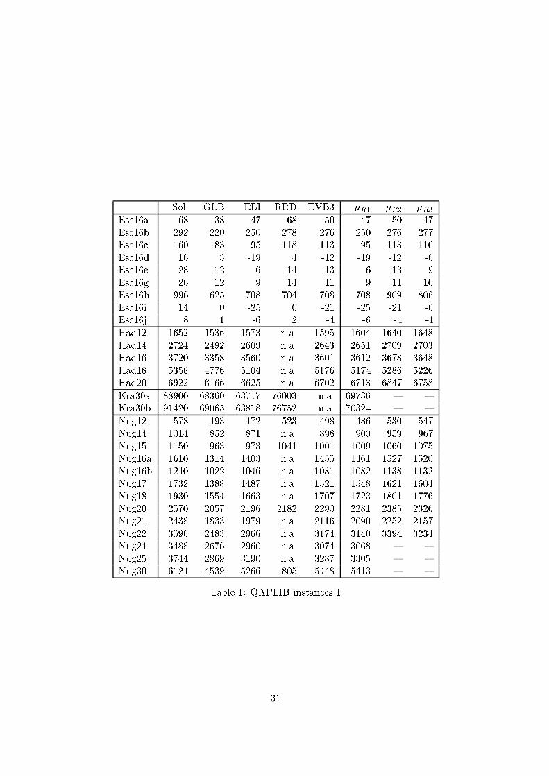
Sol. GLB ELI RRD EVB3 �R1 �R2 �R3Esc16a 68 38 47 68 50 47 50 47Esc16b 292 220 250 278 276 250 276 277Esc16c 160 83 95 118 113 95 113 110Esc16d 16 3 -19 4 -12 -19 -12 -6Esc16e 28 12 6 14 13 6 13 9Esc16g 26 12 9 14 11 9 11 10Esc16h 996 625 708 704 708 708 909 806Esc16i 14 0 -25 0 -21 -25 -21 -6Esc16j 8 1 -6 2 -4 -6 -4 -4Had12 1652 1536 1573 n.a. 1595 1604 1640 1648Had14 2724 2492 2609 n.a. 2643 2651 2709 2703Had16 3720 3358 3560 n.a. 3601 3612 3678 3648Had18 5358 4776 5104 n.a. 5176 5174 5286 5226Had20 6922 6166 6625 n.a. 6702 6713 6847 6758Kra30a 88900 68360 63717 76003 n.a. 69736 { {Kra30b 91420 69065 63818 76752 n.a. 70324 { {Nug12 578 493 472 523 498 486 530 547Nug14 1014 852 871 n.a. 898 903 959 967Nug15 1150 963 973 1041 1001 1009 1060 1075Nug16a 1610 1314 1403 n.a. 1455 1461 1527 1520Nug16b 1240 1022 1046 n.a. 1081 1082 1138 1132Nug17 1732 1388 1487 n.a. 1521 1548 1621 1604Nug18 1930 1554 1663 n.a. 1707 1723 1801 1776Nug20 2570 2057 2196 2182 2290 2281 2385 2326Nug21 2438 1833 1979 n.a. 2116 2090 2252 2157Nug22 3596 2483 2966 n.a. 3174 3140 3394 3234Nug24 3488 2676 2960 n.a. 3074 3068 { {Nug25 3744 2869 3190 n.a. 3287 3305 { {Nug30 6124 4539 5266 4805 5448 5413 { {Table 1: QAPLIB instances 131

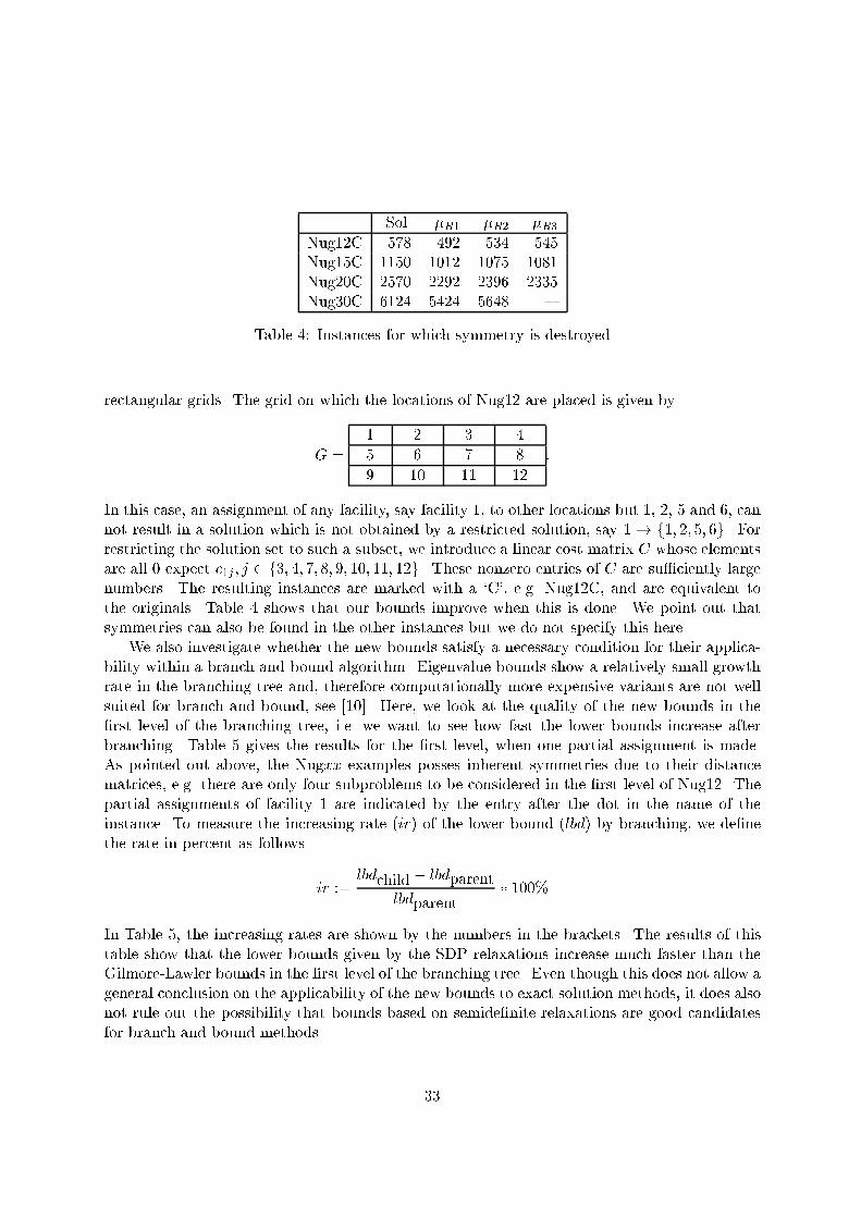
Sol. GLB ELI RRD EVB3 �R1 �R2 �R3Rou12 235528 202272 200024 224278 201337 208685 220991 227986Rou15 354210 298548 296705 324869 297958 306833 323141 324900Rou20 725522 599948 597045 643346 n.a. 615549 642448 631680Scr12 31410 27858 4727 29872 n.a. 11117 24230 27183Scr15 51140 44737 10355 49264 n.a. 17046 42094 40821Scr20 110030 86766 16113 95113 n.a. 28535 83026 59780Tai12a 224416 195918 193124 n.a. 195673 203595 215377 220938Tai15a 388214 327501 325019 n.a. 327289 333437 349476 347908Tai17a 491812 412722 408910 n.a. 410076 419619 441238 435675Tai20a 703482 580674 575831 n.a. n.a. 591994 618720 606228Tai25a 1167256 962417 956657 n.a. n.a. 974004 { {Tai30a 1818146 1504688 1500407 n.a. n.a. 1529135 { {Tho30 149936 90578 119254 100784 n.a. 125972 { {Table 2: QAPLIB instances 2Sol. GLB ELI RRD EVB3 �R1 �R2 �R3Car10ga 4954 3586 4079 n.a. 4541 4435 4853 4919Car10gb 8082 6139 7211 n.a. 7617 7600 7960 8035Car10gc 8649 7030 7837 n.a. 8233 8208 8561 8612Car10gd 8843 6840 8006 n.a. 8364 8319 8666 8780Car10ge 9571 7627 8672 n.a. 8987 8910 9349 9473Car10pa 32835 28722 -4813 n.a. n.a. 1583 12492 30359Car10pb 14282 12546 -14944 n.a. n.a. -5782 9934 13361Car10pc 14919 12296 -17140 n.a. n.a. -8040 2473 13655Esc08a 2 0 -2 0 n.a. -2 0 2Esc08b 8 1 -2 2 n.a. -2 3 6Esc08c 32 13 8 22 n.a. 9 18 30Esc08d 6 2 -2 2 n.a. -2 2 6Esc08e 2 0 -6 0 n.a. -6 -4 1Esc08f 18 9 8 18 n.a. 9 13 18Nug05 50 50 47 50 50 49 50 50Nug06 86 84 69 86 70 74 85 86Nug07 148 137 125 148 130 132 144 148Nug08 214 186 167 204 174 179 197 210Table 3: Numerical Results for old instances32

Sol. �R1 �R2 �R3Nug12C 578 492 534 545Nug15C 1150 1012 1075 1081Nug20C 2570 2292 2396 2335Nug30C 6124 5424 5648 {Table 4: Instances for which symmetry is destroyedrectangular grids. The grid on which the locations of Nug12 are placed is given byG = 1 2 3 45 6 7 89 10 11 12 :In this case, an assignment of any facility, say facility 1, to other locations but 1, 2, 5 and 6, cannot result in a solution which is not obtained by a restricted solution, say 1 ! f1; 2; 5; 6g. Forrestricting the solution set to such a subset, we introduce a linear cost matrix C whose elementsare all 0 expect c1j ; j 2 f3; 4; 7; 8; 9; 10; 11; 12g. These nonzero entries of C are su�ciently largenumbers. The resulting instances are marked with a `C', e.g. Nug12C, and are equivalent tothe originals. Table 4 shows that our bounds improve when this is done. We point out thatsymmetries can also be found in the other instances but we do not specify this here.We also investigate whether the new bounds satisfy a necessary condition for their applica-bility within a branch and bound algorithm. Eigenvalue bounds show a relatively small growthrate in the branching tree and, therefore computationally more expensive variants are not wellsuited for branch and bound, see [10]. Here, we look at the quality of the new bounds in the�rst level of the branching tree, i.e. we want to see how fast the lower bounds increase afterbranching. Table 5 gives the results for the �rst level, when one partial assignment is made.As pointed out above, the Nugxx examples posses inherent symmetries due to their distancematrices, e.g. there are only four subproblems to be considered in the �rst level of Nug12. Thepartial assignments of facility 1 are indicated by the entry after the dot in the name of theinstance. To measure the increasing rate (ir) of the lower bound (lbd) by branching, we de�nethe rate in percent as follows. ir := lbdchild � lbdparentlbdparent � 100%In Table 5, the increasing rates are shown by the numbers in the brackets. The results of thistable show that the lower bounds given by the SDP relaxations increase much faster than theGilmore-Lawler bounds in the �rst level of the branching tree. Even though this does not allow ageneral conclusion on the applicability of the new bounds to exact solution methods, it does alsonot rule out the possibility that bounds based on semide�nite relaxations are good candidatesfor branch and bound methods. 33

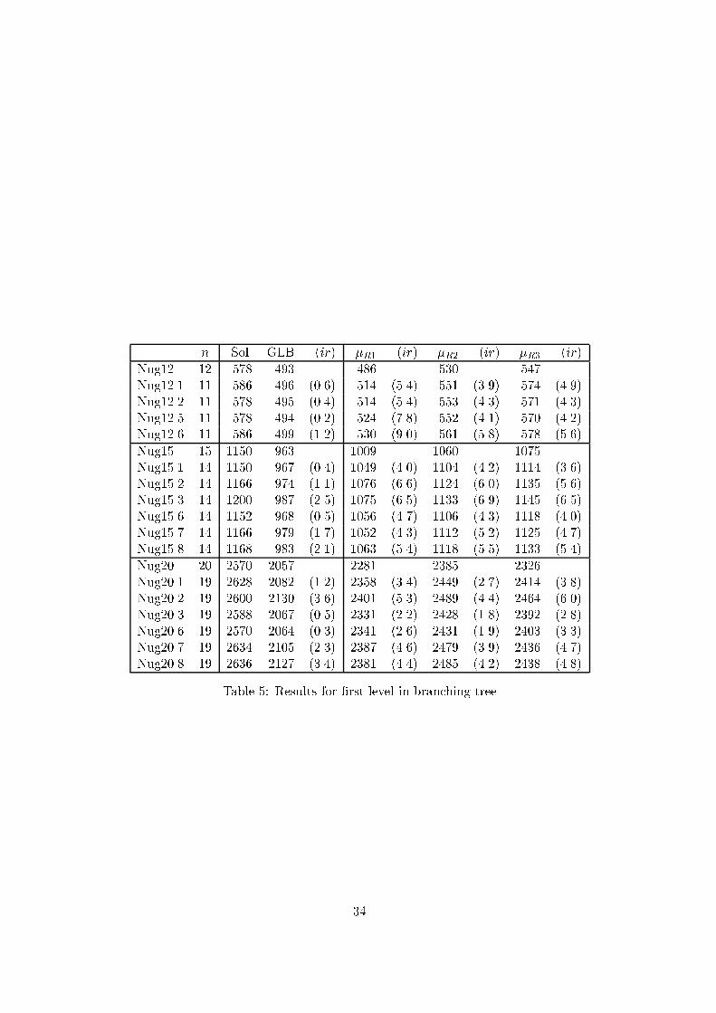
n Sol. GLB (ir) �R1 (ir) �R2 (ir) �R3 (ir)Nug12 12 578 493 486 530 547Nug12.1 11 586 496 (0.6) 514 (5.4) 551 (3.9) 574 (4.9)Nug12.2 11 578 495 (0.4) 514 (5.4) 553 (4.3) 571 (4.3)Nug12.5 11 578 494 (0.2) 524 (7.8) 552 (4.1) 570 (4.2)Nug12.6 11 586 499 (1.2) 530 (9.0) 561 (5.8) 578 (5.6)Nug15 15 1150 963 1009 1060 1075Nug15.1 14 1150 967 (0.4) 1049 (4.0) 1104 (4.2) 1114 (3.6)Nug15.2 14 1166 974 (1.1) 1076 (6.6) 1124 (6.0) 1135 (5.6)Nug15.3 14 1200 987 (2.5) 1075 (6.5) 1133 (6.9) 1145 (6.5)Nug15.6 14 1152 968 (0.5) 1056 (4.7) 1106 (4.3) 1118 (4.0)Nug15.7 14 1166 979 (1.7) 1052 (4.3) 1112 (5.2) 1125 (4.7)Nug15.8 14 1168 983 (2.1) 1063 (5.4) 1118 (5.5) 1133 (5.4)Nug20 20 2570 2057 2281 2385 2326Nug20.1 19 2628 2082 (1.2) 2358 (3.4) 2449 (2.7) 2414 (3.8)Nug20.2 19 2600 2130 (3.6) 2401 (5.3) 2489 (4.4) 2464 (6.0)Nug20.3 19 2588 2067 (0.5) 2331 (2.2) 2428 (1.8) 2392 (2.8)Nug20.6 19 2570 2064 (0.3) 2341 (2.6) 2431 (1.9) 2403 (3.3)Nug20.7 19 2634 2105 (2.3) 2387 (4.6) 2479 (3.9) 2436 (4.7)Nug20.8 19 2636 2127 (3.4) 2381 (4.4) 2485 (4.2) 2438 (4.8)Table 5: Results for �rst level in branching tree

34

Finally, the tests in the �rst level of the search tree, where the subproblems contain linearparts, and the results for the Carxx data also show that the semide�nite bounds perform wellfor instances with linear terms.AcknowledgmentsThe second author gratefully acknowledges �nancial support by the Austrian \Fond zur F�orderungder wissenschaftlichen Forschung, Erwin-Schr�odinger-Auslandsstipendium Nr. J01204-MAT".The �rst and last author would like to thank the National Science and Engineering ResearchCouncil Canada, for their support.A NotationMt the space of t� t real matricesSt the space of t� t symmetric matricest(n) n(n+1)2 , the dimension of StPt or P the cone of positive semide�nite matrices in StM1 �M2 M1 �M2 is positive semide�niteA� the adjoint of the linear operator AK+ the polar cone of K, K+ = f� : (�; k) �;8k 2 KgA � B the Hadamard product of A and BAB the Kronecker product of A and Bvec (X) the vector formed from the columns of the matrix XMat (x) the matrix formed, columnwise, from the vector XDiag (v) the diagonal matrix formed from the vector vdiag (M) the vector of the diagonal elements of the matrix ME the matrix of onese the vector of onesei the i-th unit vectorEij the matrix Eij := eieTjR(M) the range space of the matrix MN (M) the null space of the matrix M 35

E the set of matrices with row and column sums one, E := fX : Xe = XT e = egZ the set of (0,1)-matrices, Z := fX : Xij 2 f0; 1ggN the set of nonnegative matrices, N := fX : Xij � 0gO the set of orthogonal matrices, O := fX : XXT = XTX = IgYX the lifting of the matrix X, with x = vec (X);YX := " 1 xTx xxT #GJ(Y ) Gangster operator, an operator that \shoots" holes or zeros in the matrix Y , (4.1)PG(Y ) Gangster operator projected onto its range space, (4.6)Arrow (�) the Arrow operator, (2.11)B0Diag (�) the Block Diag operator, (2.12)O0Diag (�) the O� Diag operator, (2.13)arrow (�) the arrow operator, (2.15)b0diag (�) the block diag operator, (2.16)o0diag (�) the o� diag operator, (2.17)QAPE an equivalent formulation of QAP, Section 2QAPO an equivalent formulation of QAP, Section 2.2References[1] J. CLAUSEN A. BRUENGGER, M. PERREGARD, and A. MARZATTA. Joining forcesin problem solving: combining problem-speci�c knowledge and high-performance hardwareby a parallel search library to solve large-scale quadratic assignment problems. Technicalreport, University of Copenhagen, 1996.[2] W.P. ADAMS and T.A. JOHNSON. Improved linear programming-based lower bounds forthe quadratic assignment problem. In Proceedings of the DIMACS Workshop on QuadraticAssignment Problems, volume 16 of DIMACS Series in Discrete Mathematics and Theoret-ical Computer Science, pages 43{75. American Mathematical Society, 1994.[3] F. ALIZADEH, J-P.A. HAEBERLY, and M.L. OVERTON. A new primal-dual interior-point method for semide�nite programming. Technical report, Courant Institute of Mathe-matical Sciences, 1994. To appear in Proceedings of the Fifth SIAM Conference on AppliedLinear Algebra, Snowbird, Utah, June, 1994.36

[4] G.P. BARKER and D. CARLSON. Cones of diagonally dominant matrices. Paci�c J. ofMath., 57:15{32, 1975.[5] S. BOYD, L. El GHAOUI, E. FERON, and V. BALAKRISHNAN. Linear Matrix Inequal-ities in System and Control Theory, volume 15 of Studies in Applied Mathematics. SIAM,Philadelphia, PA, June 1994.[6] R.E. BURKARD. Locations with spatial interactions: the quadratic assignment problem.In P.B. Mirchandani and R.L. Francis, editors, Discrete Location Theory. John Wiley, 1991.[7] R.E. BURKARD and E. C�ELA. Quadratic and three-dimensional assignment problems.Technical Report SFB Report63, Institute of Mathematics, University of Technology Graz,1996.[8] R.E. BURKARD, S. KARISCH, and F. RENDL. A quadratic assignment problem li-brary. European Journal of Operations Research, 55:151{119, 1991. http://fmatbhp1.tu-graz.ac.at/ karisch/rep287.ps for updates.[9] T.J. CARPENTER, I. J. LUSTIG, R. E. MARSTEN, and D. F. SHANNO. Higher-orderpredictor-corrector interior point methods with application to quadratic objectives. SIAMJournal on Optimization, 3(4):696{725, 1993.[10] J. CLAUSEN, S.E. KARISCH, M. PERREGARD, and F. RENDL. On the applicabilityof lower bounds for solvin rectilinear quadratic assignment problems in parallel. Technicalreport, Institute of Mathematics, University of Technology Graz, 1996.[11] R.J. DUFFIN. In�nite programs. In A.W. Tucker, editor, Linear Equalities and RelatedSystems, pages 157{170. Princeton University Press, Princeton, NJ, 1956.[12] G. FINKE, R.E. BURKARD, and F. RENDL. Quadratic assignment problems. Annals ofDiscrete Mathematics, 31:61{82, 1987.[13] P.C. GILMORE. Optimal and suboptimal algorithms for the quadratic assignment problem.SIAM Journal on Applied Mathematics, 10:305{313, 1962.[14] M.X. GOEMANS and D.P. WILLIAMSON. .878-approximation algorithms for MAX CUTand MAX 2SAT. In ACM Symposium on Theory of Computing (STOC), 1994.[15] M.X. GOEMANS and D.P. WILLIAMSON. Improved approximation algorithms for maxi-mum cut and satis�ability problems using semide�nite programming. Journal of Associationfor Computing Machinery, 42(6):1115{1145, 1995.[16] S.W. HADLEY, F. RENDL, and H. WOLKOWICZ. A new lower bound via projection forthe quadratic assignment problem. Mathematics of Operations Research, 17:727{739, 1992.[17] C. HELMBERG. An interior point method for semide�nite programming and max-cutbounds. PhD thesis, Graz University of Technology, Austria, 1994.37

[18] C. HELMBERG, S. POLJAK, F. RENDL, and H. WOLKOWICZ. Combining semidef-inite and polyhedral relaxations to integer programs. In Proceedings of the 4th Interna-tional IPCO Conference, volume 920 of Lecture Notes in Computer Science, pages 124{134.Springer, 1995.[19] C. HELMBERG, F. RENDL, R. J. VANDERBEI, and H. WOLKOWICZ. An interiorpoint method for semide�nite programming. SIAM Journal on Optimization, pages 342{361, 1996. URL: ftp://orion.uwaterloo.ca/pub/henry/reports/sdp.ps.gz.[20] R. HORN and C. JOHNSON. Matrix Analysis. Cambridge University Press, New York,1985.[21] M. J�UNGER and V. KAIBEL. A basic study of the qap-polytope. Technical ReportTechnical Report No. 96.215, Institut f�ur Informatik, Universit�at zu K�oln, Germany, 1995.[22] S. KARISCH. Nonlinear Approaches for Quadratic Assignment and Graph Partition Prob-lems. PhD thesis, University of Graz, Graz, Austria, 1995.[23] S.E. KARISCH and F. RENDL. Lower bounds for the quadratic assignment problem viatriangle decompositions. Mathematical Programming, 71(2):137{152, 1995.[24] M. KOJIMA, S. SHINDOH, and S. HARA. Interior-point methods for the monotone linearcomplementarity problem in symmetric matrices. Technical report, Dept. of InformationSciences, Tokyo Institute of Technology, Tokyo, Japan, 1994.[25] S. KRUK and H. WOLKOWICZ. SQ2P, sequential quadratic constrained quadratic pro-gramming. Research report, University of Waterloo, Waterloo, Ontario, In progress.[26] E. LAWLER. The quadratic assignment problem. Management Science, 9:586{599, 1963.[27] L. LOV�ASZ and A. SCHRIJVER. Cones of matrices and set-functions and 0-1 optimization.SIAM Journal on Optimization, 1(2):166{190, 1991.[28] I. J. LUSTIG, R. E. MARSTEN, and D. F. SHANNO. On implementing Mehrotra'spredictor{corrector interior point method for linear programming. SIAM Journal on Opti-mization, 2(3):435{449, 1992.[29] C.E. NUGENT, T.E. VOLLMAN, and J. RUML. An experimental comparison of techniquesfor the assignment of facilities to locations. Operations Research, 16:150{173, 1968.[30] P. PARDALOS, F. RENDL, and H. WOLKOWICZ. The quadratic assignment problem:A survey and recent developments. In Proceedings of the DIMACS Workshop on QuadraticAssignment Problems, volume 16 of DIMACS Series in Discrete Mathematics and Theoret-ical Computer Science, pages 1{41. American Mathematical Society, 1994.[31] G. PATAKI. Algorithms for cone-optimization problems and semi-de�nite programming.Technical report, GSIA Carnegie Mellon University, Pittsburgh, PA, 1993.38

[32] S. POLJAK, F. RENDL, and H. WOLKOWICZ. A recipe for semide�nite relaxation for(0,1)-quadratic programming. Journal of Global Optimization, 7:51{73, 1995.[33] L. PORTUGAL, M.G.C. RESENDE, G. VEIGA, and J. JUDICE. A truncated primal-infeasible dual-fesible network interior point method. Technical report, Universidade deCoimbra, Coimbra, Portugal, 1994.[34] K.G. Ramakrishnan, M.G.C. RESENDE, and P.M. PARDALOS. A branch and boundalgorithm for the quadratic assignment problem using a lower bound based on linear pro-gramming. In C. Floudas and P.M. PARDALOS, editors, State of the Art in Global Opti-mization: Computational Methods and Applications. Kluwer Academic Publishers, 1995.[35] M. RAMANA, L. TUNCEL, and H. WOLKOWICZ. Strong duality for semide�-nite programming. SIAM Journal on Optimization, page to appear, 1997. URL:ftp://orion.uwaterloo.ca/pub/henry/reports/strongdual.ps.gz.[36] F. RENDL and H. WOLKOWICZ. Applications of parametric programming and eigenvaluemaximization to the quadratic assignment problem. Mathematical Programming, 53:63{78,1992.[37] M.G.C. RESENDE, K.G. RAMAKRISHNAN, and Z. DREZNER. Computing lower boundsfor the quadratic assignment problem with an interior point algorithm for linear program-ming. Operations Research, 43(5):781{791, 1995.[38] M. RIJAL. Scheduling, design and assignment problems with quadratic costs. PhD thesis,New York University, New York, USA, 1995.[39] S. SAHNI and T. GONZALES. P-complete approximation problems. Journal of ACM,23:555{565, 1976.[40] H.D. SHERALI and W.P. ADAMS. Computational advances using the reformulation-linearlization technique (rlt) to solve discrete and continuous nonconvex problems. Optima,49:1{6, 1996.[41] L. VANDENBERGHE and S. BOYD. Primal-dual potential reduction method for problemsinvolving matrix inequalities. Math. Programming, 69(1):205{236, 1995.[42] L. VANDENBERGHE and S. BOYD. Semide�nite programming. SIAM Review, 38:49{95,1996.[43] H. WOLKOWICZ. Some applications of optimization in matrix theory. Linear Algebra andits Applications, 40:101{118, 1981.39