Lundstrom ECE 305 S15

ECE-305: Spring 2015

Semiconductor Equations: II

Professor Mark Lundstrom Electrical and Computer Engineering

Purdue University, West Lafayette, IN USA lundstro@purdue.edu

2/9/15

Pierret, Semiconductor Device Fundamentals (SDF) pp. 120-138

Lundstrom ECE 305 S15 2

outline 1.  Drift-diffusion current

2.  The continuity equation

3.  Quasi-Fermi levels

4.  Generation - Recombination

5.  Minority carrier diffusion equation

✓

✓

✓

drift- diffusion equation

3

!J p = pqµ p

!E − qDp

!∇p

!Jn = nqµn

!E + qDn

!∇n

current = drift current + diffusion current

!J =!J p +

!Jn

total current = electron current + hole current

Dp µ p = Dn µn = kBT q

continuity equation for holes

4

∂p∂t

= −∇i

!Jpq

+Gp − Rp

in-flow

out-flow

∂p ∂t

recombination generation

in-flow - out-flow + G - R ∂p∂t

=

s.s. no G-R

5

∂p∂t

= −∇ i

!Jpq+Gp − Rp →∇ i

!Jp = 0 →

!Jp is constant

in-flow

out-flow

∂p ∂t

recombination generation

!Jp x( )

!Jp x + Δx( ) =

!Jp x( )

optical generation

6

EC

EV

E = hf > EG EG

Δn

Δp

Low level injection in an n-type semiconductor:

n ≈ n0

p ≈ Δp >> p0

Δp << n0( )

equilibrium vs. non-equilibrium

7

EC

EV

EG

n0 = 1017 cm-3

p0 =ni2

n0= 103 cm-3

EF

EC

EV

n = 1017 cm-3

p ≈ Δp >> p0 cm-3

Fp

Fn

n-type / equilibrium n-type / low-level injection

equilibrium vs. non-equilibrium

8

n0 = nieEF−Ei( ) kBT

p0 = nieEi−EF( ) kBT

n = nieFn−Ei( ) kBT

p = nieEi−Fp( ) kBT

n0p0 = ni2 np = ni

2e Fn−Fp( ) kBT ≠ ni2

equilibrium non-equilibrium

f0 =1

1+ e E−EF( ) kBTfc =

11+ e E−Fn( ) kBT

1− fv = 1−1

1+ e E−Fp( ) kBT

current and QFL’s

9

J px = pqµ pE x − qDp dp dx p = nie

Ei−Fp( ) kBT

dpdx

= nieEi−Fp( ) kBT × 1

kBTdEi

dx−dFpdx

⎛⎝⎜

⎞⎠⎟= pkBT

dEi

dx−dFpdx

⎛⎝⎜

⎞⎠⎟

dEi

dx= qE x

J px = pµ p dFp dx

Lundstrom ECE 305 S15 10

outline 1.  Drift-diffusion current

2.  The continuity equation

3.  Quasi-Fermi levels

4.  Generation - Recombination

5.  Minority carrier diffusion equation

✓

✓

✓

Lundstrom ECE 305 S15 11

recombination

∂p∂t

= −∇i

!Jpq

+Gp − Rp

turn the light off

12

EC

EV

EG

Δn = 1010 cm-3

Δp = 1010 cm-3

Question: What happens?

Answer: The system returns to equilibrium.

How long does it take? A time known as the “minority carrier lifetime”.

τ p sec

carrier recombination

13

EC

EV

EG

Δn = 1010 cm-3

Δp = 1010 cm-3

Rp = − ∂p∂t R−G

≈ Δpτ p

(low-level injection)

R-G processes

14

Fig. 3.15a from R.F. Pierret, Semiconductor Device Fundamentals

Shockley-Read-Hall (SRH)

continuity equation for holes

15

∂p∂t

= −∇i

!Jpq

+Gp − Rp

in-flow

out-flow

∂p ∂t

recombination generation

“the semiconductor equations”

16

∂ p∂t

= −∇i

!Jpq

⎛

⎝⎜⎞

⎠⎟+Gp − Rp

∂n∂t

= −∇i!Jn−q

⎛⎝⎜

⎞⎠⎟+Gn − Rn

0 = −∇i ε

!E( ) + ρ

Three equations in three unknowns:

p!r( ), n !r( ), V !r( )

!J p = pqµ p

!E − qDp

!∇p = pµ p

!∇ Fp q( )

!Jn = nqµn

!E + qDn

!∇n = nµn

!∇ Fn q( )

ρ = q p − n + N D

+ − N A−( )

!

E !r( ) = ∇V !r( )

Lundstrom ECE 305 S15 17

outline 1.  Drift-diffusion current

2.  The continuity equation

3.  Quasi-Fermi levels

4.  Generation - Recombination

5.  Minority carrier diffusion equation

✓

✓

✓ ✓

minority carrier diffusion equation

18

∂ p∂t

= −∇i

!Jpq

⎛

⎝⎜⎞

⎠⎟+Gp − Rp

∂ p∂t

= − ddx

Jpxq

⎛⎝⎜

⎞⎠⎟+GL − Rp (1D, generation by light)

∂Δp∂t

= − ddx

−qDp dΔp dxq

⎛⎝⎜

⎞⎠⎟+GL −

Δpτ p

(low-level injection, no electric field)

∂Δp∂t

= Dpd 2Δpdx2

− Δpτ p

+GL (Dp spatially uniform)

(hole continuity equation)

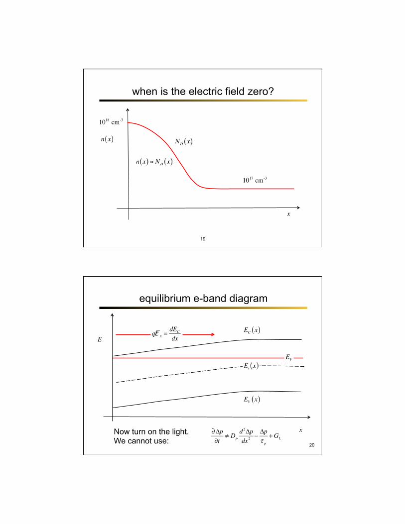
when is the electric field zero?

19

x

n x( ) ND x( )

1017 cm-3

1018 cm-3

n x( ) ≈ ND x( )

equilibrium e-band diagram

20

EF

EC x( )

EV x( )

Ei x( )

x

E qE x =

dEC

dx

∂Δp∂t

≠ Dpd 2Δpdx2

− Δpτ p

+GLNow turn on the light. We cannot use:

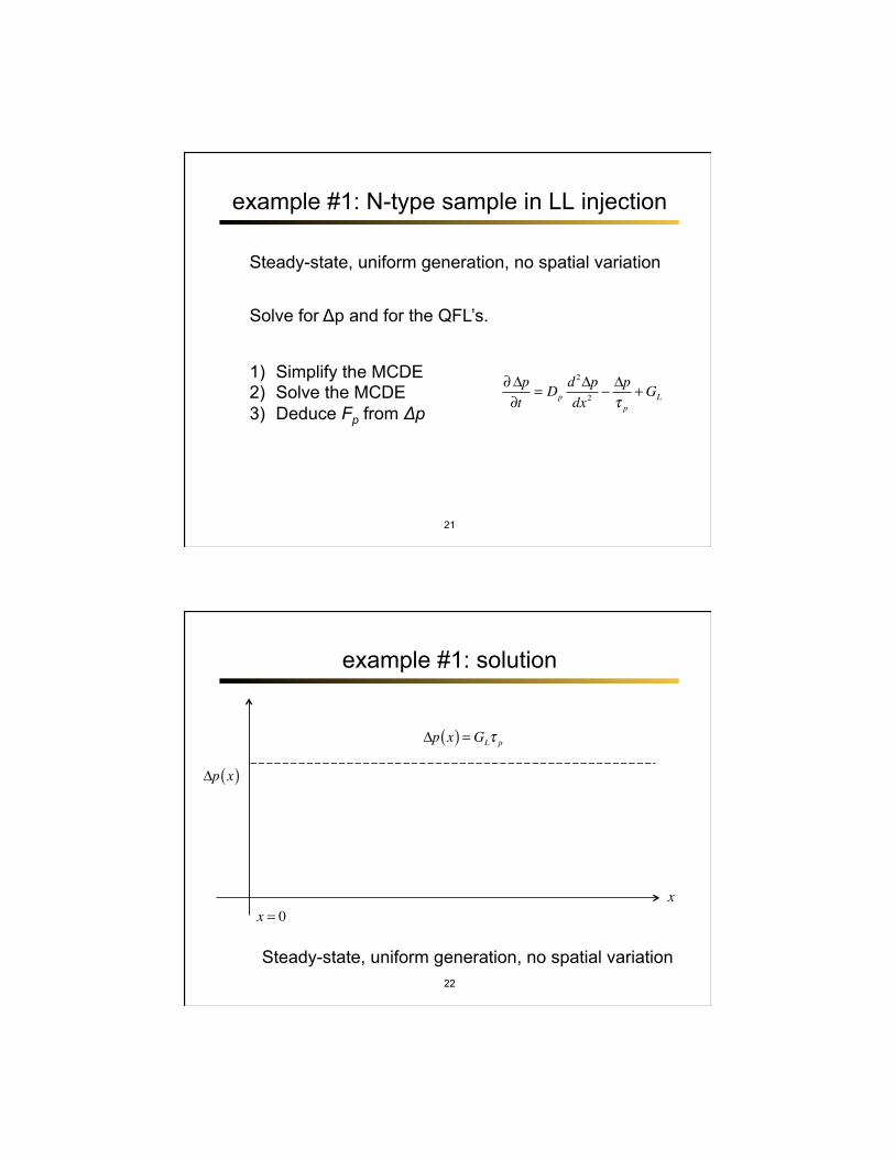
example #1: N-type sample in LL injection

21

Steady-state, uniform generation, no spatial variation

Solve for Δp and for the QFL’s.

1)  Simplify the MCDE 2)  Solve the MCDE 3)  Deduce Fp from Δp

∂Δp∂t

= Dpd 2Δpdx2

− Δpτ p

+GL

example #1: solution

22

x

Δp x( )

Δp x( ) = GLτ p

x = 0

Steady-state, uniform generation, no spatial variation

example #2

23

Solve for Δp and for the QFL’s.

1)  Simplify the MCDE 2)  Solve the MCDE 3)  Deduce Fp from Δp

∂Δp∂t

= Dpd 2Δpdx2

− Δpτ p

+GL

Now turn off the light. Transient, no generation, no spatial variation

example #2

24

x

Δp x( )

Δp t = 0( ) = GLτ p

x = 0

transient, no generation, no spatial variation

Δp t( ) = Δp t = 0( )e− t /τ p

How do the QFL’s vary with time?

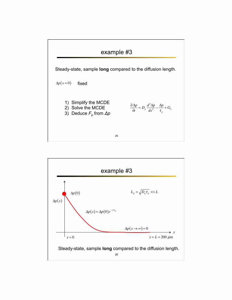
example #3

25

Steady-state, sample long compared to the diffusion length.

fixed Δp x = 0( )

1)  Simplify the MCDE 2)  Solve the MCDE 3)  Deduce Fp from Δp

∂Δp∂t

= Dpd 2Δpdx2

− Δpτ p

+GL

example #3

26

x

Δp x( )

Δp x→∞( ) = 0

Δp 0( )

Δp x( ) = Δp 0( )e− x/Lp

x = L = 200 µmx = 0

Lp = Dpτ p << L

Steady-state, sample long compared to the diffusion length.

Lundstrom ECE 305 S15 27

outline 1.  Drift-diffusion current

2.  The continuity equation

3.  Quasi-Fermi levels

4.  Generation - Recombination

5.  Minority carrier diffusion equation

✓

✓

✓ ✓