SEMI-SUPERVISED LEARNING

Jasneet Sabharwal jasneet.sabharwal@sfu.ca

Types of Learning

• Supervised Learning - Uses only labelled data for training a classifier.

• Semi-Supervised Learning - Uses both labelled and unlabelled data for training a classifier.

• Unsupervised Learning - Uses only unlabelled data.

Why do we need Semi-Supervised Learning?

• Labelled data is hard to get

• Annotation takes time and is boring

• Domain experts are required

• Undergraduates are on a holiday

• Unlabelled data is cheap

Generative Models

• p(x,y) = p(y) p(x|y), where p(x|y) is an identifiable mixture model (example - Gaussian Mixture Model)

• With large unlabelled data, we can identify mixture components and then we

• Only require one labelled example per mixture component to identify the mixture distribution

Generative Models

−5 −4 −3 −2 −1 0 1 2 3 4 5−5

−4

−3

−2

−1

0

1

2

3

4

5

−5 −4 −3 −2 −1 0 1 2 3 4 5−5

−4

−3

−2

−1

0

1

2

3

4

5

(a) labeled data (b) labeled and unlabeled data (small dots)

−5 −4 −3 −2 −1 0 1 2 3 4 5−5

−4

−3

−2

−1

0

1

2

3

4

5

−5 −4 −3 −2 −1 0 1 2 3 4 5−5

−4

−3

−2

−1

0

1

2

3

4

5

(c) model learned from labeled data (d) model learned from labeled and unlabeled data

Figure 1: In a binary classification problem, if we assume each class has a Gaussiandistribution, then we can use unlabeled data to help parameter estimation.

8

• Note

• If mixture model assumptions are correct then unlabelled data will improve accuracy. - Castelli & Cover, 1995; Castelli & Cover, 1996; Ratsaby & Venkatesh, 1995

• If mixture models are wrong then unlabelled data may hurt accuracy. - Cozmen et. al. 2003

−6 −4 −2 0 2 4 6−6

−4

−2

0

2

4

6

Class 1

Class 2

−6 −4 −2 0 2 4 6−6

−4

−2

0

2

4

6

−6 −4 −2 0 2 4 6−6

−4

−2

0

2

4

6

(a) Horizontal class separation (b) High probability (c) Low probability

Figure 3: If the model is wrong, higher likelihood may lead to lower classificationaccuracy. For example, (a) is clearly not generated from two Gaussian. If we insistthat each class is a single Gaussian, (b) will have higher probability than (c). But(b) has around 50% accuracy, while (c)’s is much better.

2.3 EM Local Maxima

Even if the mixture model assumption is correct, in practice mixture componentsare identified by the Expectation-Maximization (EM) algorithm (Dempster et al.,1977). EM is prone to local maxima. If a local maximum is far from the globalmaximum, unlabeled data may again hurt learning. Remedies include smart choiceof starting point by active learning (Nigam, 2001).

2.4 Cluster-and-Label

We shall also mention that instead of using an probabilistic generative mixturemodel, some approaches employ various clustering algorithms to cluster the wholedataset, then label each cluster with labeled data, e.g. (Demiriz et al., 1999) (Daraet al., 2002). Although they can perform well if the particular clustering algorithmsmatch the true data distribution, these approaches are hard to analyze due to theiralgorithmic nature.

2.5 Fisher kernel for discriminative learning

Another approach for semi-supervised learning with generative models is to con-vert data into a feature representation determined by the generative model. The newfeature representation is then fed into a standard discriminative classifier. Holubet al. (2005) used this approach for image categorization. First a generative mix-ture model is trained, one component per class. At this stage the unlabeled data canbe incorporated via EM, which is the same as in previous subsections. Howeverinstead of directly using the generative model for classification, each labeled ex-ample is converted into a fixed-length Fisher score vector, i.e. the derivatives of loglikelihood w.r.t. model parameters, for all component models (Jaakkola & Haus-sler, 1998). These Fisher score vectors are then used in a discriminative classifier

10

Generative Models• Identifying Mixture Components

• Expectation Maximization (Dempster et. al., 1977) is generally used

• Prone to local maxima

• If local maxima far away from global maxima then unlabelled data may hurt learning

Fischer Kernel for Discriminative Learning

• Train generative mixture models (one component per class)

• Use EM to incorporate unlabelled data

• For each component model, convert labelled examples into fixed length Fisher score vector (derivatives of log likelihood w.r.t model parameters)

• Use Fisher score vectors in discriminative classifier (example - SVM)

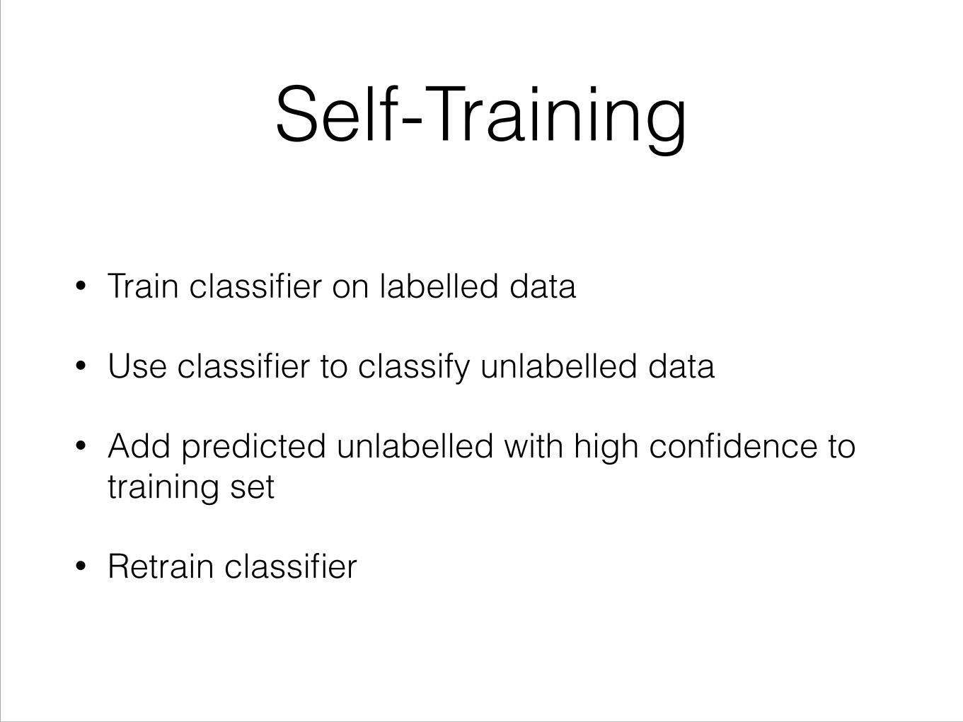
Self-Training

• Train classifier on labelled data

• Use classifier to classify unlabelled data

• Add predicted unlabelled with high confidence to training set

• Retrain classifier

Self-Training• Advantages of Self-Training

• Simplest form of semi-supervised learning method

• Wrapper method, applied to other existing classifiers

• Frequently used in real time tasks in NLP (example - Named Entity Recognition)

• Disadvantages of Self-Training

• Mistakes can re-enforce themselves

Co-Training• Assumptions

• Features can be split into two sets.

• Each sub-feature set is sufficient to train a classifier.

• Sub-feature sets are conditionally independent given the class.

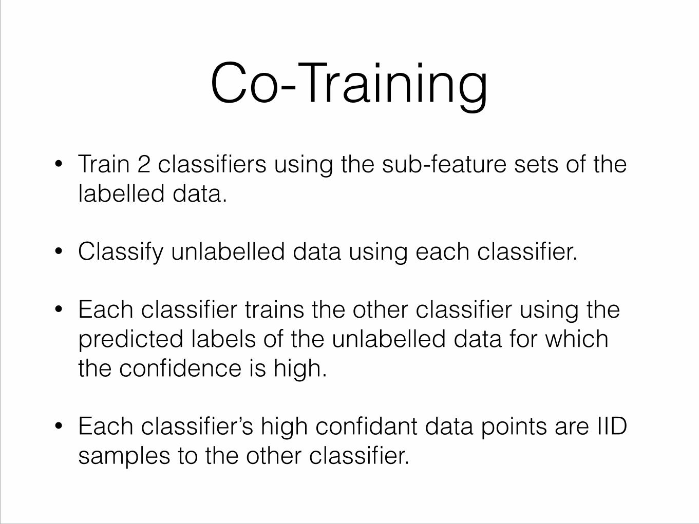
Co-Training• Train 2 classifiers using the sub-feature sets of the

labelled data.

• Classify unlabelled data using each classifier.

• Each classifier trains the other classifier using the predicted labels of the unlabelled data for which the confidence is high.

• Each classifier’s high confidant data points are IID samples to the other classifier.

Co-Training

• Works well when conditional independence holds.

• Only works when one classifier correctly labels a data that the other classifier misclassified.

• If no natural feature split is present, then randomly split features into two parts.

Co-Training• Alternative to feature splitting

• Goldman and Zhou (2000) - Use two different learners but use full features for both. Then use one learner’s high confidence data points as training for other learner.

• Zhou and Goldman (2004) - Ensemble of learners with different inductive bias.

• Zhou and Li (2005) - Tri-learning

Semi-Supervised vs Transductive Learning

• Semi-Supervised Learning

• Uses both labelled and unlabelled data

• Contrasts Supervised or Unsupervised learning

• Transductive Learning

• Only works on labelled and unlabelled data

• Cannot handle unseen data

Transductive Learning• Inductive approach - Use labelled data and

train a supervised classifier.

• Only 5 labelled points

• Tough to capture the structure of data

• Transductive approach - Consider all points

• Label the unlabelled according to clusters that they belong to

• If unseen data points are added, then entire transductive algorithm needs to be repeated

Transductive SVMs

• SVMs only use labelled data and we find maximum margin boundary

• Use of both labelled and unlabelled data

• Goal - Find labelling of unlabelled data such that linear boundary has maximum margin on both labelled and unlabelled data

Transductive SVMs

share parameters. Notice p(x) is usually all we can get from unlabeled data. It isbelieved that if p(x) and p(y|x) do not share parameters, semi-supervised learningcannot help. This point is emphasized in (Seeger, 2001).

Transductive support vector machines (TSVMs)1 builds the connection be-tween p(x) and the discriminative decision boundary by not putting the boundaryin high density regions. TSVM is an extension of standard support vector machineswith unlabeled data. In a standard SVM only the labeled data is used, and the goalis to find a maximum margin linear boundary in the Reproducing Kernel HilbertSpace. In a TSVM the unlabeled data is also used. The goal is to find a labeling ofthe unlabeled data, so that a linear boundary has the maximum margin on both theoriginal labeled data and the (now labeled) unlabeled data. The decision bound-ary has the smallest generalization error bound on unlabeled data (Vapnik, 1998).Intuitively, unlabeled data guides the linear boundary away from dense regions.

+

+

+

++

−

−

−

−

Figure 5: In TSVM, U helps to put the decision boundary in sparse regions. Withlabeled data only, the maximummargin boundary is plotted with dotted lines. Withunlabeled data (black dots), the maximum margin boundary would be the one withsolid lines.

However finding the exact transductive SVM solution is NP-hard. Major efforthas focused on efficient approximation algorithms. Early algorithms (Bennett &Demiriz, 1999) (Demirez & Bennett, 2000) (Fung & Mangasarian, 1999) eithercannot handle more than a few hundred unlabeled examples, or did not do so inexperiments. The SVM-light TSVM implementation (Joachims, 1999) is the firstwidely used software.

De Bie and Cristianini (De Bie & Cristianini, 2004; De Bie & Cristianini,2006b) relax the TSVM training problem, and transductive learning problems ingeneral to semi-definite programming (SDP). The basic idea is to work with thebinary label matrix of rank 1, and relax it by a positive semi-definite matrix withoutthe rank constraint. The paper also includes a speech up trick to solve median-sized

1In recent papers, TSVMs are also called Semi-Supervised Support Vector Machines (S3VM),because the learned classifiers can in fact be used inductively to predict on unseen data.

14

Unlabelled data guides the linear boundary away from dense regions

Thank You