Semi-Leptonic Decay Of Lambda-B In The Standard Model And ...

University of Mississippi University of Mississippi

eGrove eGrove

Electronic Theses and Dissertations Graduate School

2015

Semi-Leptonic Decay Of Lambda-B In The Standard Model And Semi-Leptonic Decay Of Lambda-B In The Standard Model And

With New Physics With New Physics

Wanwei Wu University of Mississippi

Follow this and additional works at: https://egrove.olemiss.edu/etd

Part of the Physics Commons

Recommended Citation Recommended Citation Wu, Wanwei, "Semi-Leptonic Decay Of Lambda-B In The Standard Model And With New Physics" (2015). Electronic Theses and Dissertations. 761. https://egrove.olemiss.edu/etd/761

This Thesis is brought to you for free and open access by the Graduate School at eGrove. It has been accepted for inclusion in Electronic Theses and Dissertations by an authorized administrator of eGrove. For more information, please contact [email protected].

https://egrove.olemiss.edu/

https://egrove.olemiss.edu/etd

https://egrove.olemiss.edu/gradschool

https://egrove.olemiss.edu/etd?utm_source=egrove.olemiss.edu%2Fetd%2F761&utm_medium=PDF&utm_campaign=PDFCoverPages

http://network.bepress.com/hgg/discipline/193?utm_source=egrove.olemiss.edu%2Fetd%2F761&utm_medium=PDF&utm_campaign=PDFCoverPages

https://egrove.olemiss.edu/etd/761?utm_source=egrove.olemiss.edu%2Fetd%2F761&utm_medium=PDF&utm_campaign=PDFCoverPages

mailto:[email protected]

SEMI-LEPTONIC DECAY OF LAMBDA-B

IN THE STANDARD MODEL AND WITH NEW PHYSICS

A Thesis

presented in partial fulfillment of requirements

for the degree of Master of Science

in the Department of Physics and Astronomy

The University of Mississippi

by

WANWEI WU

April 2015

ABSTRACT

Heavy quark decays provide a very advantageous investigation to test the Standard

Model (SM). Recently, promising experiments with b quark, as well as the analysis of the

huge data sets produced at the B factories, have led to an increasing study and sensitive

measurements of relative b quark decays. In this thesis, I calculate various observables in

the semi-leptonic decay process Λb → Λcτ ντ both in the SM and in the presence of New

Physics (NP) operators with different Lorentz structures. The results are relevant for the

coming measurement of this semi-leptonic decay at LHC b experiment in CERN, and also

provide theoretical predictions to refine the physics beyond the SM.

ii

ACKNOWLEDGEMENTS

I would like to express my sincere gratitude to my advisor Dr. Alakabha Datta for

his continuous support. Without his guidance, I could not have finished this thesis. His

valuable advice and comments, as well as his patience and immense knowledge, helped me

in all the time with my study and research. I would like to thank the rest of my thesis

committees: Dr. Lucien Cremaldi and Dr. Luca Bombelli for their insightful comments and

precious time.

Also, my sincere thanks go to Dr. Emanuele Berti, Dr. Donald Summers, Dr. Breese

Quinn, Dr. Murugeswaran Duraisamy, Dr. Preet Sharma, and Shanmuka Shivashankara. In

particular, I would like to thank Hongkai Liu for studying together and helpful discussions.

In addition, I would like to thank my parents. As simple and kind-hearted farmers,

they try to understand and support me all the way.

iii

CONTENTS

ABSTRACT ii

ACKNOWLEDGEMENTS iii

LIST OF TABLES vi

LIST OF FIGURES vii

1 INTRODUCTION 1

1.1 Standard Model . . . . . . . . . . . . . . . . . . . . . . . . . . . . . . . . . . 2

1.2 Weak Interactions . . . . . . . . . . . . . . . . . . . . . . . . . . . . . . . . . 3

1.3 QCD . . . . . . . . . . . . . . . . . . . . . . . . . . . . . . . . . . . . . . . . 4

2 FORMALISM 5

2.1 Decay Process . . . . . . . . . . . . . . . . . . . . . . . . . . . . . . . . . . . 5

2.2 Partial Decay Rate . . . . . . . . . . . . . . . . . . . . . . . . . . . . . . . . 6

2.3 Feynman Amplitude . . . . . . . . . . . . . . . . . . . . . . . . . . . . . . . 6

2.3.1 SM . . . . . . . . . . . . . . . . . . . . . . . . . . . . . . . . . . . . . 8

2.3.2 NP Effects . . . . . . . . . . . . . . . . . . . . . . . . . . . . . . . . . 8

2.4 Observables . . . . . . . . . . . . . . . . . . . . . . . . . . . . . . . . . . . . 10

3 NUMERICAL RESULTS 11

3.1 NP Couplings . . . . . . . . . . . . . . . . . . . . . . . . . . . . . . . . . . . 11

3.2 Form Factors . . . . . . . . . . . . . . . . . . . . . . . . . . . . . . . . . . . 12

iv

3.3 Result Graphs . . . . . . . . . . . . . . . . . . . . . . . . . . . . . . . . . . . 13

4 CONCLUSION 18

BIBLIOGRAPHY 19

LIST OF APPENDICES 22

A NP OPERATORS EXPRESSED IN TERMS OF FORM FACTORS 23

B KINEMATICS 25

C B → D∗ FORM FACTORS 28

C.1 B → D∗τ−νµ Angular Distribution . . . . . . . . . . . . . . . . . . . . . . . 29

C.2 B → D∗τ−νµ Form Factors . . . . . . . . . . . . . . . . . . . . . . . . . . . . 29

C.3 B → D∗ Kinematics . . . . . . . . . . . . . . . . . . . . . . . . . . . . . . . 30

C.4 B → D∗ Amplitudes . . . . . . . . . . . . . . . . . . . . . . . . . . . . . . . 32

D B → Dτντ FORM FACTORS 35

D.1 B → Dτντ Angular Distribution . . . . . . . . . . . . . . . . . . . . . . . . . 36

D.2 B → Dτντ Amplitudes . . . . . . . . . . . . . . . . . . . . . . . . . . . . . . 36

D.3 B → Dτντ Form Factors . . . . . . . . . . . . . . . . . . . . . . . . . . . . . 36

VITA 38

v

LIST OF TABLES

3.1 Various Choices of Form Factors (t = q2) . . . . . . . . . . . . . . . . . . . . 13

3.2 Values of RΛb in the SM . . . . . . . . . . . . . . . . . . . . . . . . . . . . . 13

3.3 Minimum and Maximum Values for the Averaged RΛb . . . . . . . . . . . . . 17

vi

LIST OF FIGURES

1.1 The SM of Elementary Particles (matter fermions in the first three genera-

tions, gauge bosons in the fourth column, and the Higgs boson in the fifth) . 3

2.1 Λb Decay Process in the SM and with NP(some new mediating particles) . . 6

3.1 B → D(∗)τ−ντ Decay Process . . . . . . . . . . . . . . . . . . . . . . . . . . 11

3.2 The figures show the constraints on the NP couplings taken one at a time at

the 95% CL limit. When the couplings contribute to both R(D) and R(D∗)

the green areas indicate constraints from R(D) and the orange ones from

R(D∗). . . . . . . . . . . . . . . . . . . . . . . . . . . . . . . . . . . . . . . 12

3.3 The graphs on the left-side (right-side) show the compared results between

the standard model and new physics with only gL (gR) present. The top and

bottom row of graphs depict RΛb = BR[Λb → Λcτ ντ ]/BR[Λb → Λc`ν`] and the

ratio of differential distributions BΛb(q2) = dΓ

dq2(Λb → Λcτ ντ )/

dΓdq2

(Λb → Λc`ν`)

as a function of q2, respectively for the various form factors in Table 3.1. The

middle graphs depict the average differential decay rate with respect to q2 for

the process Λb → Λcτ ντ . Some representative values of the couplings have

been chosen. . . . . . . . . . . . . . . . . . . . . . . . . . . . . . . . . . . . 14

vii

3.4 The figures show the compared results between the standard model and new

physics with only gS present. The top and bottom row of graphs depict RΛb =

BR[Λb → Λcτ ντ ]/BR[Λb → Λc`ν`] and the ratio of differential distributions

BΛb(q2) = dΓ


dΓdq2

(Λb → Λc`ν`) as a function of q2, respectively

for the various form factors in Table 3.1. The middle graphs depict the average

differential decay rate with respect to q2 for the process Λb → Λcτ ντ . Some

representative values of the couplings have been chosen. . . . . . . . . . . . 15

3.5 The figures show the compared results between the standard model and new

physics with only gP present. The top and bottom row of graphs depict RΛb =

BR[Λb → Λcτ ντ ]/BR[Λb → Λc`ν`] and the ratio of differential distributions

BΛb(q2) = dΓ


dΓdq2

(Λb → Λc`ν`) as a function of q2, respectively

for the various form factors in Table 3.1. The middle graphs depict the average

differential decay rate with respect to q2 for the process Λb → Λcτ ντ . Some

representative values of the couplings have been chosen. . . . . . . . . . . . 16

viii

CHAPTER 1

INTRODUCTION

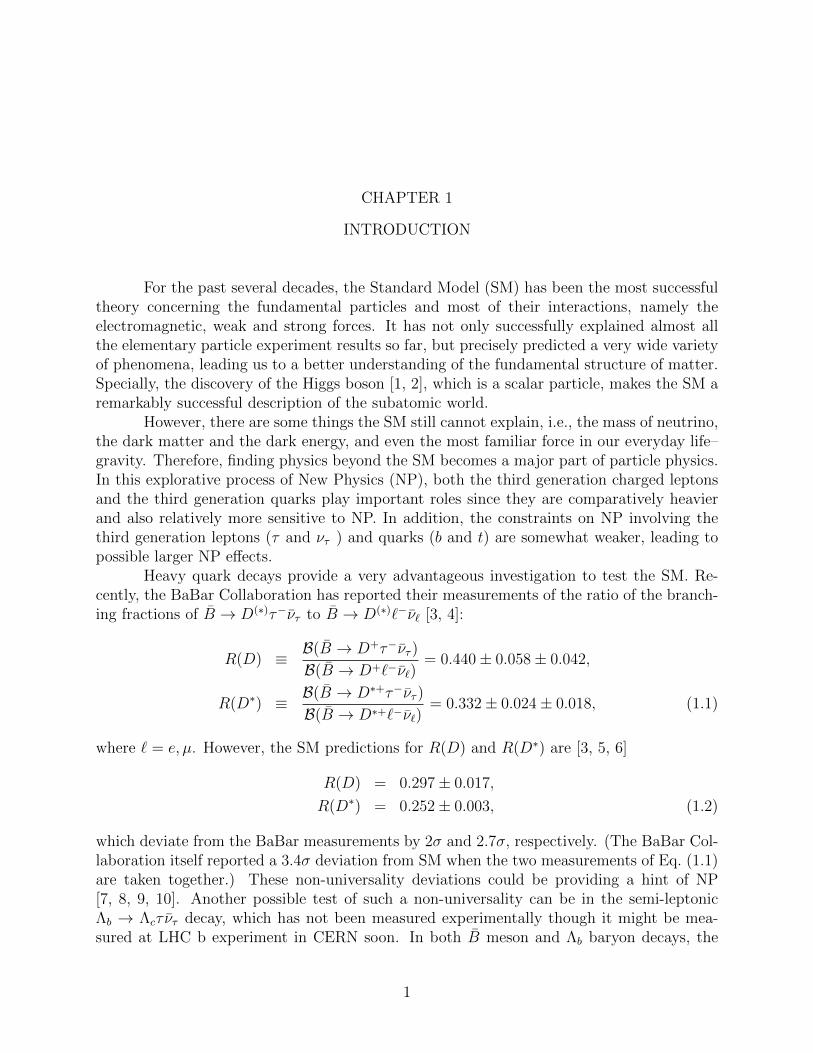
For the past several decades, the Standard Model (SM) has been the most successfultheory concerning the fundamental particles and most of their interactions, namely theelectromagnetic, weak and strong forces. It has not only successfully explained almost allthe elementary particle experiment results so far, but precisely predicted a very wide varietyof phenomena, leading us to a better understanding of the fundamental structure of matter.Specially, the discovery of the Higgs boson [1, 2], which is a scalar particle, makes the SM aremarkably successful description of the subatomic world.

However, there are some things the SM still cannot explain, i.e., the mass of neutrino,the dark matter and the dark energy, and even the most familiar force in our everyday life–gravity. Therefore, finding physics beyond the SM becomes a major part of particle physics.In this explorative process of New Physics (NP), both the third generation charged leptonsand the third generation quarks play important roles since they are comparatively heavierand also relatively more sensitive to NP. In addition, the constraints on NP involving thethird generation leptons (τ and ντ ) and quarks (b and t) are somewhat weaker, leading topossible larger NP effects.

Heavy quark decays provide a very advantageous investigation to test the SM. Re-cently, the BaBar Collaboration has reported their measurements of the ratio of the branch-ing fractions of B → D(∗)τ−ντ to B → D(∗)`−ν` [3, 4]:

R(D) ≡ B(B → D+τ−ντ )

B(B → D+`−ν`)= 0.440± 0.058± 0.042,

R(D∗) ≡ B(B → D∗+τ−ντ )

B(B → D∗+`−ν`)= 0.332± 0.024± 0.018, (1.1)

where ` = e, µ. However, the SM predictions for R(D) and R(D∗) are [3, 5, 6]

R(D) = 0.297± 0.017,

R(D∗) = 0.252± 0.003, (1.2)

which deviate from the BaBar measurements by 2σ and 2.7σ, respectively. (The BaBar Col-laboration itself reported a 3.4σ deviation from SM when the two measurements of Eq. (1.1)are taken together.) These non-universality deviations could be providing a hint of NP[7, 8, 9, 10]. Another possible test of such a non-universality can be in the semi-leptonicΛb → Λcτ ντ decay, which has not been measured experimentally though it might be mea-sured at LHC b experiment in CERN soon. In both B meson and Λb baryon decays, the

1

underlying quark level transition b→ cτ−ντ can be probed, as both B meson and Λb baryoncontain a b quark which will decay here.

In this thesis, I calculate various observables in the semi-leptonic decay process Λb →Λcτ ντ both in the SM and in the presence of NP operators with different Lorentz structuresby using constraints on the NP couplings obtained by using Eq. (1.1). Since the calculationsinvolve the structures of both B meson and Λb baryon, the Quantum Chromodynamics(QCD) for the strong interactions between quarks and gluons (specially, the form factors),will be briefly introduced as well as the SM and the weak interactions.

1.1 Standard Model

The Standard Model of particle physics, formulated in the 1970s, is a theory offundamental particles and their interactions. It is based on the quantum theory of fields andprovides the most accurate description of nature at the subatomic level so far. According tothis model, all matter is built from a small number of fundamental spin-1

2particles, called

fermions : six quarks and six leptons, which follow the Fermi-Dirac statistics; while thecarriers of the interactions are characterized as bosons, which possess integer spin (either 0or 1 ) and follow the Bose-Einstein statistics. There are seventeen named particles in theSM, which are organized in Fig. 1.1. The Higgs boson, as the last particle in the SM, wasdiscovered in 2012 [1, 2].

There are four known fundamental interactions in the universe: the gravitational,the electromagnetic, the weak and the strong interactions. They work over different rangesand have different strengths. Gravity, acting between all types of particle, is the weakestbut it has an infinite range. It is supposedly mediated by exchange of a spin-2 boson, thegraviton, which has not been observed. Even though it is universal and is dominant onthe scale of the universe, gravity is not included in the SM because it is much weaker thanthe other forces and can be neglected at the level of individual subatomic particles. Theelectromagnetic interaction acts between all charged particles and is mediated by photon (γ)exchange. It also has infinite range but it is many times stronger than gravity. The weak andstrong interactions are effective only over a very short range and dominate only at the levelof subatomic particles. The weak interaction is associated with the exchange of elementaryspin-1 bosons between quarks and/or leptons. These mediators are W± and Z0 bosons, withmasses of order 100 times the proton mass. The strong interaction, as its name suggests, isthe strongest of all four fundamental interactions. It is responsible for binding the quarksin the neutron and proton, and the neutrons and protons within nuclei. The strong force ismediated by spin-1, massless particles known as gluons, which couple to color charge, ratherlike the photons couple to electromagnetic charge.

Fermions are fundamental matter particles in the SM. These twelve particles (sixleptons and six quarks) can be grouped into three generations. The lightest and most stableparticles make up the first generation, whereas the heavier and less stable particles belongto the second and third generations. The leptons carry integral electric charge. The chargedleptons are the electron, muon and tau, while the neutral leptons are the correspondingneutrinos. A different “flavour” of neutrino is paired with each “flavour” of charged lepton,as indicated by the subscript, i.e., (e, νe), (µ, νµ) and (τ , ντ ). The charged muon and tau

2

Figure 1.1: The SM of Elementary Particles (matter fermions in the first three generations,gauge bosons in the fourth column, and the Higgs boson in the fifth)

are both unstable and decay spontaneously to electrons, neutrinos and other particles. Themean lifetime of the muon is 2.2× 10−6 s, that of the tau only 2.9× 10−13 s. Neutrinos werepostulated by Pauli in 1930 in order to account for the energy and momentum missing in theprocess of nuclear β-decay. They experience the weak interactions only. The quarks carryfractional electric charges, of +2

3e or −1

3e. The quark “flavour” is denoted by a symbol: u

for ‘up’, d for ‘down’, s for ‘strange’, c for ‘charmed’, b for ‘bottom’ and t for ‘top’. Whileleptons exist as free particles, quarks are not found to do so. The bound states of quarks arecalled hadrons, which can be categorized into two families: baryons (made of three quarks)and mesons (made of one quark and one anti-quark). Each quark carries one of the threecolors(or color charges): r, g and b. Quarks are bound together by gluons, which are alsocolored. Fig.1.1 shows that the three lepton pairs are exactly matched by the three quarkpairs.

1.2 Weak Interactions

The weak interaction is mediated by three massive bosons, the charged W± andthe neutral Z0. The W+ and W− are anti-particles of each other, while the Z0, like thephoton, is its own anti-particle. Depending on whether leptons and/or hadrons are involved,the weak interaction can be conventionally divided into three categories: (i) purely leptonicprocesses, e.g., µ− → e− + νe + νµ, (ii) semi-leptonic processes involving both hadrons andleptons, e.g., neutron β-decay n → p + e− + νe, and (iii) purely hadronic processes, e.g.,Λ → p + π−. Perturbation theory is valid for weak and electromagnetic interactions. In

3

the 1960s, a theory of electroweak interactions was developed by Sheldon Glashow, AbdusSalam and Steven Weinberg that can unify the electromagnetic and weak interactions.

So far, the experimental data on a wide range of leptonic and semi-leptonic processesare consistent with the assumption that the lepton fields enter the interaction only in thecombinations

Jα(x) =∑l

ψl(x)γα(1− γ5)ψνl(x),

J†α(x) =∑l

ψνl(x)γα(1− γ5)ψl(x), (1.3)

where Jα(x) and J†α(x) are called leptonic currents, l = e, µ, τ , ψl and ψνl are the corre-sponding quantized fields in Eq. (1.3). We can describe the weak interaction as due tothe transmission of quanta, i.e., W±. For example, the interaction Hamiltonian density ofquantum electrodynamics (QED), according to the intermediate vector boson (IVB) theorycan be given by

HI(x) = gWJα†(x)Wα(x) + gWJ

α(x)W †α(x), (1.4)

where gW is a dimensionless coupling constant and the field Wα(x) describes the W bosonsin Eq. (1.4). This interaction is known as a “V-A”interaction, since the current Jα(x) canbe written as the difference of a vector part (γµ) and an axial vector part (γµγ5).

1.3 QCD

Quantum chromodynamics (QCD) is the standard theory to describe the strong in-teractions, in which the color quantum number has been introduced as an extra degree offreedom. The color charge of a quark has three possible values, r, g and b, while anti-quarkscarry anti-colors, r, g and b. The mediating bosons of the quark-quark interactions are calledgluons, each carrying a color and an anti-color and postulated to belong to an octet of states.

Quarks and gluons are observed indirectly, which means that the evidence of theirexistence inside hadrons exists but these particles have not been observed singly. Experi-ments to study the strong interactions are performed with hadrons, not with the quarks andgluons that are described by quantum field theory (QFT). To explore or determine the quarkand gluon structure of hadrons, structure functions are introduced to give the properties of acertain particle interaction without including all of the underlying physics. The experimentaltechnique is to measure the angular distribution of some processes and compare it to thatfrom a point particle, then the structure of the hadron can be deduced from some form fac-tors(functions of the transferred momentum square). As an example, a charge distributionwith electrons can be probed by measuring the cross section for scattering electrons:

dσ

dΩ= (

dσ

dΩ)point|F (q)|2, (1.5)

where q is the transferred momentum and F (q) is the corresponding form factor.

4

CHAPTER 2

FORMALISM

The physics of the decay process Λb → Λcτ ντ can be described by an effective Hamilto-nian. In the presence of NP, the effective Hamiltonian for the quark-level transition b→ cl−νlcan be written in the form [11, 12]

Heff =GFVcb√

2

[cγµ(1− γ5)b+ gLcγµ(1− γ5)b+ gRcγµ(1 + γ5)b

]lγµ(1− γ5)νl

+[gS cb+ gP cγ5b

]l(1− γ5)νl + h.c

, (2.1)

where GF = 1.1663787 × 10−5GeV −2 is the Fermi coupling constant, Vcb is the Cabibbo-Kobayashi-Maskawa (CKM) matrix element, gL,R,S,P are NP couplings and I use σµν =i[γµ, γν ]/2. In this thesis, I have assumed the neutrinos to be always left chiral and theNP effect is mainly for the τ lepton. Here, I do not consider tensor operators in my work.Moreover, I do not assume any relation between b → ul−νl and b → cl−νl transitions andhence the analysis does not include constraints from B → τντ . As it is expected, the SMeffective Hamiltonian corresponds to gL = gR = gS = gP = 0.

In Refs. [9, 10], the authors had parametrized the NP in terms of the couplings gS,gP , gV = gR + gL and gA = gR − gL while in this thesis I have used gL and gR instead of gVand gA to align the analysis closer to realistic models [13]. The couplings gL,R,P contributeto R(D∗) while gL,R,S contribute to R(D). The NP couplings are considered one at a timeand the constraints on these couplings are obtained from R(D(∗)).

2.1 Decay Process

Λb is a baryon of three quarks: u, d and b, while Λc is a baryon with u, d and c quarks.The semi-leptonic decay process under consideration is

Λb(p)→ τ−(p1) + ντ (p2) + Λc(p3),

where p, p1, p2 and p3 are four energy-momentum vectors respectively. Technically, thedecay process Λb → Λcτ ντ transits the b-quark to the c-quark, as is shown in Fig. 2.1. Inthe SM, the mediating boson is W−, which will subsequently decay into a τ lepton and τanti-neutrino. With NP, instead of W−, the mediator can be a new particle, i.e., anothernew vector particle W ′− or a scalar (or Higgs) particle H−. I will consider these NP effectsand compare the results with those from the SM.

5

Figure 2.1: Λb Decay Process in the SM and with NP(some new mediating particles)

2.2 Partial Decay Rate

The partial decay rate of a particle of mass m into n bodies in its rest frame is givenby

dΓ =(2π)4

2m|M |2dΦn(p; p1, ..., pn), (2.2)

where M is the Feynman amplitude and dΦn is an element of n-body phase space given by

dΦn(p; p1, ..., pn) = δ4(p−n∑i=1

pi)n∏i=1

d3pi(2π)32Ei

. (2.3)

This phase space element can be generated recursively

dΦn(p; p1, ..., pn) = dΦj(q; p1, ..., pj)× dΦn−j+1(p; q, pj+1, ..., pn)(2π)3dq2, (2.4)

where q2 = (∑j

i=1 Ei)2 − |

∑ji=1pi|2. This form is particularly useful in the case where a

particle decays into another particle that subsequently decays, e.g., Λb → ΛcW− → Λcτ

−ντ .A useful method to achieve the integration of dΓ is given in Appendix B.

2.3 Feynman Amplitude

The Feynman amplitude M includes all the physical processes. In fact, the key pointto calculate the decay rate is to evaluate the |M |2 appearing in Eq. (2.2).

The total Feynman amplitude here is

Mtotal = MSM +MgL +MgR +MgS +MgP , (2.5)

where MgL,R,S,P are corresponding to the NP couplings gL,R,S,P .

6

In the SM, the Feynman amplitude for this process is given by

MSM =GFVcb√

2LµHµ, (2.6)

where the leptonic and hadronic currents are

Lµ = uτ (p1)γµ(1− γ5)vντ (p2),

Hµ = 〈Λc|cγµ(1− γ5)|Λb〉. (2.7)

The hadronic current is expressed in terms of six form factors,

〈Λc|cγµb|Λb〉 = uΛc(f1γµ + if2σµνqν + f3qµ)uΛb ,

〈Λc|cγµγ5b|〉Λb = uΛc(g1γµγ5 + ig2σµνqνγ5 + g3qµγ5)uΛb . (2.8)

Here q = p− p3 is the transferred momentum and the form factors are functions of q2.When NP operators appear, we can obtain the hadronic current by considering the

following relations:

qµ〈Λc|cγµb|Λb〉 = qµuλc(f1γµ + if2σµνqν + f3qµ)uλb ,

qµ〈Λc|cγµγ5b|Λb〉 = qµuλc(g1γµγ5 + ig2σµνqνγ5 + g3qµγ5)uλb . (2.9)

Using the equations of motion, we’ll finally get (the details are shown in Appendix A)

〈Λc|cb|Λb〉 = uΛc(f1/q

mb −mc

+ f3q2

mb −mc

)uΛb ,

〈Λc|cγ5b|Λb〉 = uΛc(−g1/qγ5

mb +mc

− g3q2γ5

mb +mc

)uΛb . (2.10)

where mb and mc are the masses of the b quark and c quark.To obtain the corresponding unpolarized decay rate, we need to average |M |2 over all

initial polarization states and sum it over all final polarization states,

¯|M |2 =1

2

∑spin

|M |2

=G2f |Vcb|2

4LµνHµν , (2.11)

where Lµν stands for the leptonic part and Hµν stands for the hadronic part (Lµν and Hµν

are tensors in the SM and with a vector NP effect). In the following part of this section, Iwill give the details of how to obtain ¯|M |2 both in the SM and with NP effects. However,from Eq. (2.5) we know that there should be some crossing terms between the SM and NPeffects. We are not going to consider the crossing term between two different NP effects sincewe just consider one NP coupling at a time. To get the final result form of Eq. (2.11), wehave to consider the kinematics of the decay process. The kinematics here is considered inthe rest frame of Λb, and details are given in Appendix B.

7

2.3.1 SMIn the SM, the leptonic tensor in Eq. (2.11) is∑

spin

LµνSM =∑spin

[uτ (p1)γµ(1− γ5)vντ (p2)][vντ (p2)γν(1− γ5)uτ (p1)]

= Tr[( /p1 +m1)γµ(1− γ5)( /p2 −m2)γν(1− γ5)]

= 8(−gµνp1 · p2 − iεµνρσp1ρp2σ + pµ1pν2 + pν1p

µ2). (2.12)

Here, m1 is the mass of τ lepton and m2 is the mass of tau neutrino. I already treat theneutrino as massless, m2 → 0. The hadronic tensor in Eq. (2.11) in the SM is∑

spin

HSMµν =∑spin

HSMµHSM∗ν

=∑spin

(A−B)(A∗ −B∗)

=∑spin

(AA∗ − AB∗ −BA∗ +BB∗), (2.13)

where

A = uλc(f1γµ + if2σµνqν + f3qµ)uλb ,

B = uλc(g1γµγ5 + ig2σµνqνγ5 + g3qµγ5)uλb ,

A∗ = uλb(f1γν − if2σνδqδ + f3qν)uλc ,

B∗ = uλb(g1γνγ5 + ig2σνδqδγ5 − g3qνγ5)uλc . (2.14)

2.3.2 NP EffectsLet’s consider the NP effects for one NP coupling at a time and set the others to zero.

For the vector NP effects, we consider the case with only gL present and the case with onlygR present. For the scalar/pseudoscalar NP effects, we consider the case with only gS or gPpresent.

For the vector NP effect with only gL present, the NP coupling will appear in thehadronic current part in the Feynman amplitude and the leptonic current part is the sameas that in the SM. Therefore, the leptonic tensor LµνgL = LµνSM has the form in Eq. (2.12). Thehadronic tensor with only gL present is

HSM+gLµν =∑spin

HSM+gLµHSM+gL∗ν

=∑spin

(HSMµHSM∗ν +HSMµHgL

∗ν +HgLµHSM

∗ν +HgLµHgL

∗ν)

=∑spin

(1 + g∗L + gL + |gL|2)(A−B)(A∗ −B∗). (2.15)

With the gR present, we will have LµνgR = LµνSM for the same reason as with gL. The corre-

8

sponding hadronic tensor is

HSM+gRµν =∑spin

HSM+gRµHSM+gR∗ν

=∑spin

(HSMµHSM∗ν +HSMµHgR

∗ν +HgRµHSM

∗ν +HgRµHgR

∗ν)

=∑spin

[(A−B)(A∗ −B∗) + g∗R(A−B)(A∗ +B∗)

+gR(A+B)(A∗ −B∗) + |gR|2(A+B)(A∗ +B∗)]. (2.16)

The A, B, A∗ and B∗ appearing in Eq. (2.15) and Eq. (2.16) are given in Eq. (2.14).For the scalar and pseudoscalar NP effects, the Feynman amplitudes are given by

MgS = gSGFVcb√

2LSC,

MgP = gPGFVcb√

2LSD, (2.17)

where LS is the leptonic current, C and D are the corresponding hadronic currents. Then

the ¯|M |2 in Eq. (2.11) with NP effect with only gS present becomes

¯|M |2SM+gS=

1

2

∑spin

(|MSM |2 +MSMM∗gS

+MgSM∗SM + |MgS |2)

=G2f |Vcb|2

4

∑spin

[LL∗(A−B)(A∗ −B∗) + g∗SLL∗S(A−B)C∗

+gSLSL∗C(A∗ −B∗) + |gS|2LSL∗SCC∗], (2.18)

and the ¯|M |2 with only gP present becomes

¯|M |2SM+gP=

1

2

∑spin

(|MSM |2 +MSMM∗gP

+MgPM∗SM + |MgP |2)

=G2f |Vcb|2

4

∑spin

[LL∗(A−B)(A∗ −B∗) + g∗PLL∗S(A−B)D∗

+gPLSL∗D(A∗ −B∗) + |gP |2LSL∗SDD∗]. (2.19)

Here, L is the leptonic current in Eq. (2.7) and L∗ is its conjugate part. In addition,

LS = uτ (p1)(1− γ5)vντ (p2),

C = uλc(f1/q

mb −mc

+ f3q2

mb −mc

)uλb ,

D = uλc(−g1/qγ5

mb +mc

− g3q2γ5

mb +mc

)uλb , (2.20)

9

and their corresponding conjugate parts are

L∗S = vντ (p2)(1 + γ5)uτ (p1),

C∗ = uλb(f1/q

mb −mc

+ f3q2

mb −mc

)uλc ,

D∗ = uλb(−g1/qγ5

mb +mc

+ g3q2γ5

mb +mc

)uλc . (2.21)

The cross terms between two different NP couplings are zero since we consider oneNP coupling at a time, as Eq. (2.5) indicates.

2.4 Observables

The calculation is based on integration of Eq. (2.2), which gives us the decay rate ofthe process Λb → Λcτ ντ directly. In this thesis, we’ll define the following observables.

RΛb =BR[Λb → Λcτ ντ ]

BR[Λb → Λc`ν`]. (2.22)

Here ` represents µ or e. The branching ratio BR for a specific decay process is defined by

BRi =Γi∑

Γi, (2.23)

where Γi is the decay rate for this process and∑

Γi is the total decay rate.The differential distributions with respect to the transferred momentum square q2 will

be shown in the results (dΓ/dq2). Also, we will define the ratio of differential distributions

BΛb(q2) =

dΓ[Λb → Λcτ ντ ]

dq2

/dΓ[Λb → Λc`ν`]

dq2. (2.24)

The results will show that these observables are not very sensitive to variations in thehadronic form factors.

10

CHAPTER 3

NUMERICAL RESULTS

In this section, I will present the constraints on the NP couplings, then I will discussand show the form factors used in this work. Finally, I will present the result graphs of theobservables defined in section 2.4.

3.1 NP Couplings

The NP constraints on the NP couplings are obtained from R(D(∗)) in Eq. (1.1) andEq. (1.2). The relative decay processes are

B → Dτ−ντ , and B → D∗τ−ντ .

The two main reasons we use the NP constraints from the decay process B → D(∗)τ−ντ hereare: the experimental results of R(D(∗)) from the BaBar Collaboration deviating from thosein SM provide a hint of NP [3, 4], and both Λb baryon decay and B meson decay involve thetransition b → cl−νl, as shown in Fig. 2.1 and in Fig. 3.1. The formalism to constrain theNP couplings here is

Rexp = RSM

(1 + gNP

MNPM∗SM

|MSM |2+ g∗NP

MSMM∗NP

|MSM |2+ |gNP |2

|MNP |2

|MSM |2), (3.1)

where gNP stands for gL,R,S,P .

Figure 3.1: B → D(∗)τ−ντ Decay Process

11

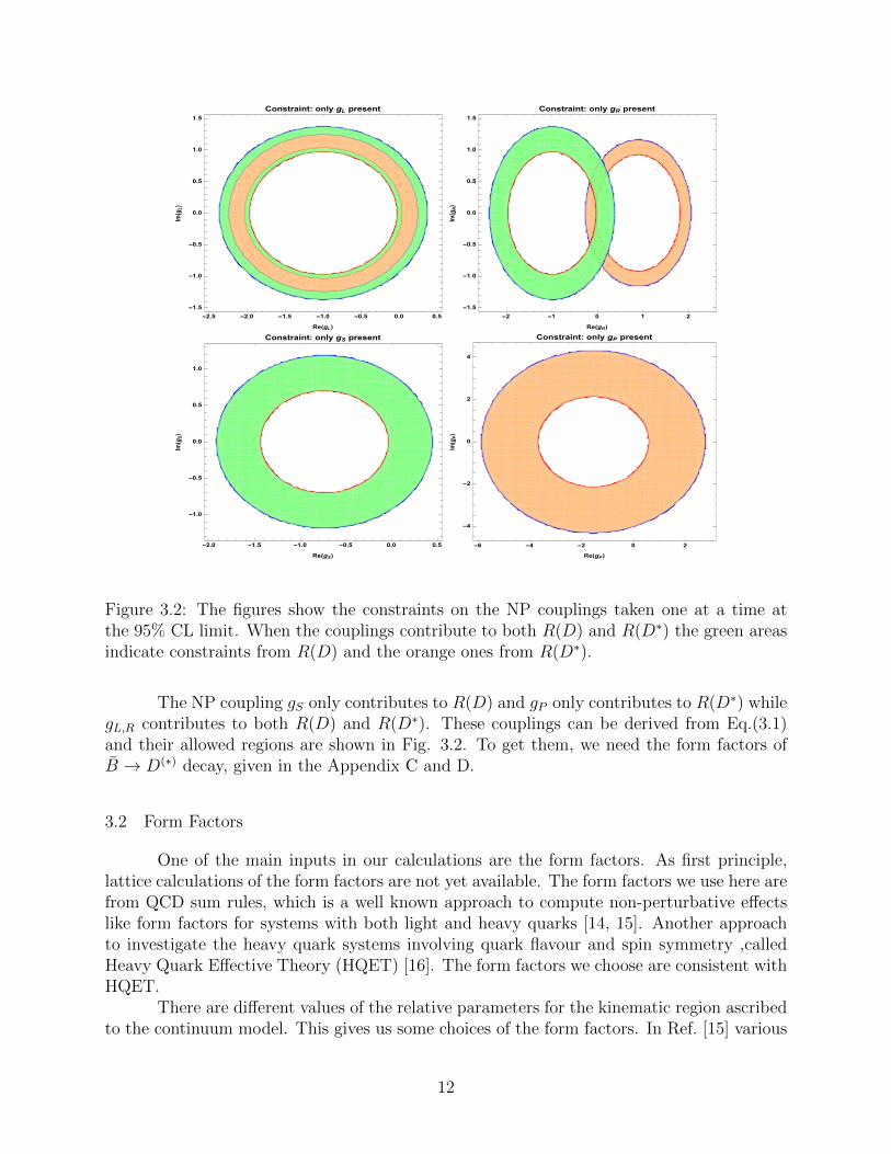
Figure 3.2: The figures show the constraints on the NP couplings taken one at a time atthe 95% CL limit. When the couplings contribute to both R(D) and R(D∗) the green areasindicate constraints from R(D) and the orange ones from R(D∗).

The NP coupling gS only contributes to R(D) and gP only contributes to R(D∗) whilegL,R contributes to both R(D) and R(D∗). These couplings can be derived from Eq.(3.1)and their allowed regions are shown in Fig. 3.2. To get them, we need the form factors ofB → D(∗) decay, given in the Appendix C and D.

3.2 Form Factors

One of the main inputs in our calculations are the form factors. As first principle,lattice calculations of the form factors are not yet available. The form factors we use here arefrom QCD sum rules, which is a well known approach to compute non-perturbative effectslike form factors for systems with both light and heavy quarks [14, 15]. Another approachto investigate the heavy quark systems involving quark flavour and spin symmetry ,calledHeavy Quark Effective Theory (HQET) [16]. The form factors we choose are consistent withHQET.

There are different values of the relative parameters for the kinematic region ascribedto the continuum model. This gives us some choices of the form factors. In Ref. [15] various

12

parametrizations of the form factors are given. They are shown below.

continuum model κ F V1 (t) = f1 F V

2 (t)(GeV −1) = f2

rectangular 1 6.66/(20.27− t) −0.21/(15.15− t)rectangular 2 8.13/(22.50− t) −0.22/(13.63− t)triangular 3 13.74/(26.68− t) −0.41/(18.65− t)triangular 4 16.17/(29.12− t) −0.45/(19.04− t)

Table 3.1: Various Choices of Form Factors (t = q2)

The form factors in Table 3.1 are based on four continuum models indicated byκ = 1, 2, 3, 4. However, the differences of the results from these models are very small, whichcan be shown in the result graphs. Moreover, these form factors in Table 3.1 satisfy theHQET relation in the mb →∞ limit. They have the following relations:

f1 = g1, f2 = g2, f3 = g3 = 0. (3.2)

3.3 Result Graphs

I have used the following masses in my calculations. The masses of the particles arem = 5.6195 GeV, mτ = 1.77682 GeV, mµ = 0.10565837 GeV, m3 = 2.28646 GeV, mb = 4.66GeV and mc = 1.275 GeV [17]. In the following I will present the results for observables RΛb ,dΓ/dq2 and BΛb(q

2). For the first and third observables I use different models of the formfactors given in Table 3.1. For the differential distribution dΓ/dq2, I present the averageresults over the form factors.

continuum model 1 2 3 4 Average Ref. [19] Ref. [20]RΛb(SM) 0.31 0.29 0.28 0.27 0.29 0.29 0.31

Table 3.2: Values of RΛb in the SM

In Table 3.2, the prediction for RΛb in the SM are given for the various choices of theform factors in Table 3.1. I also compare our results with other calculations of this quantityby other groups using different form factors. The average value we found for RΛb in the SMis RΛb,SM = 0.29. This agrees very well with values for this quantity obtained in Ref. [19],which uses a covariant confined quark model for the form factors, and Ref. [20] which usesthe form factor model in Ref. [21]. These results indicate that the ratio RΛb is largely freefrom form factor uncertainties making it an excellent probe to find new physics.

Now I give the discussions of the results. From Eq. (2.5), we can make some generalobservations. We start with the case where only gL is present. In this case the NP Feynmanamplitude has the same structure as the SM one and the total Feynman amplitude is justthe SM amplitude modified by the factor (1 + gL). Hence, if only gL is present, then

RΛb = RΛbSM |1 + gL|2. (3.3)

Therefore, in this case, RΛb ≥ RΛbSM and we find the range of RΛb to be 0.31 v 0.44. The

13

Figure 3.3: The graphs on the left-side (right-side) show the compared results between thestandard model and new physics with only gL (gR) present. The top and bottom row ofgraphs depict RΛb = BR[Λb → Λcτ ντ ]/BR[Λb → Λc`ν`] and the ratio of differential distri-butions BΛb(q

2) = dΓdq2

(Λb → Λcτ ντ )/dΓdq2

(Λb → Λc`ν`) as a function of q2, respectively forthe various form factors in Table 3.1. The middle graphs depict the average differentialdecay rate with respect to q2 for the process Λb → Λcτ ντ . Some representative values of thecouplings have been chosen.

14

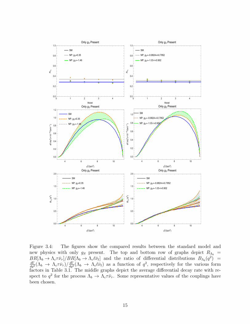
Figure 3.4: The figures show the compared results between the standard model andnew physics with only gS present. The top and bottom row of graphs depict RΛb =BR[Λb → Λcτ ντ ]/BR[Λb → Λc`ν`] and the ratio of differential distributions BΛb(q

2) =dΓdq2


(Λb → Λc`ν`) as a function of q2, respectively for the various formfactors in Table 3.1. The middle graphs depict the average differential decay rate with re-spect to q2 for the process Λb → Λcτ ντ . Some representative values of the couplings havebeen chosen.

15

Figure 3.5: The figures show the compared results between the standard model andnew physics with only gP present. The top and bottom row of graphs depict RΛb =BR[Λb → Λcτ ντ ]/BR[Λb → Λc`ν`] and the ratio of differential distributions BΛb(q

2) =dΓdq2


(Λb → Λc`ν`) as a function of q2, respectively for the various formfactors in Table 3.1. The middle graphs depict the average differential decay rate with re-spect to q2 for the process Λb → Λcτ ντ . Some representative values of the couplings havebeen chosen.

16

shape of the differential distribution dΓ/dq2 is the same as in the SM. In the left-side figuresof Fig. 3.3, we show the plots for RΛb , dΓ/dq2 and BΛb(q

2) when only gL is present. We thenconsider the case where only gR is present. If only gR is present, then from Eq. (2.13) andEq. (2.16) we can deduce that no clear relation between RΛb and RΛbSM can be obtained inthis case. However, for the allowed gR couplings, we find RΛb is greater than the SM valueand is in the range 0.30 v 0.51. The shape of the differential distribution dΓ/dq2 is alsothe same as that of the SM. In the right-side figures of Fig. 3.3, we show the plots for RΛb ,dΓ/dq2 and BΛb(q

2) when only gR is present.We now move to the case when only gS,P are present. Using Eq. (2.5), Eq. (2.6) and

Eq. (2.17), we can write

RΛb = RΛbSM + |gS|2AS + 2Re(gS)BS,

RΛb = RΛbSM + |gP |2AP + 2Re(gP )BP , (3.4)

since the physics of the the decay process only underlies in the Feyman amplitudes. Thequantities AS,P and BS,P depend on masses and form factors and they are positive. Hence,for Re(gP ) ≥ 0 or Re(gS) ≥ 0, RΛb is always greater than or equal to RΛbSM . But, forRe(gP ) < 0 or Re(gS) < 0, RΛb can be possibly less than the SM value. However, for thegiven constraints on gS here, we can make RΛb only slightly less than the SM value whilefor gP it is always larger than the SM value. We find RΛb is in the range 0.28 v 0.36 whenonly gS is present and in the range 0.30 v 0.42 when only gP is present. In Fig. 3.4 we showthe plots for RΛb , dΓ/dq2 and BΛb(q

2) when only gS is present. The shape of the differentialdistribution dΓ/dq2 can be different from that of the SM. In Fig. 3.5 we show the plotsfor RΛb , dΓ/dq2 and BΛb(q

2) when only gP is present. In this case also the shape of thedifferential distribution dΓ/dq2 can be different from that of the SM.

NP RΛb,min RΛb,max

Only gL 0.31, gL = −0.065 + 0.447 i 0.44, gL = −0.144 + 0.903 iOnly gR 0.30, gR = −0.033 + 0.119 i 0.51, gR = 0.182 + 0.914 iOnly gS 0.28, gS = −1.442 0.36, gS = 0.443Only gP 0.30, gP = 0.587 0.42, gP = −5.859

Table 3.3: Minimum and Maximum Values for the Averaged RΛb .

In Table 3.3, we show the minimum and maximum values for the averaged RΛb withthe corresponding NP couplings.

17

CHAPTER 4

CONCLUSION

In this thesis, I calculated the SM and the NP predictions for the decay Λb → Λcτ ντ .Motivation to study this decay comes from the recent hints of lepton flavor non-universality

observed by the BaBar Collaboration in R(D(∗)) ≡ B(B→D(∗)+τ−ντ )

B(B→D(∗)+`−ν`)(` = e, µ). I used a

general parametrization of the NP operators and fixed the new physics couplings from theexperimental measurements of R(D) and R(D∗). The predictions for RΛb (Eq.(2.22)), dΓ

dq2,

and BΛb(q2) (Eq.(2.24)) are made by taking one of the various NP couplings at a time. We

found the interesting results that gL,R,P couplings gave predictions larger than the SM valuesfor all the three observables while the gS couplings gave predictions which could be larger orsmaller than the SM values.

This thesis is related to our recent work of Λb → Λcτ ντ decay [22].

18

BIBLIOGRAPHY

19

BIBLIOGRAPHY

[1] G. Aad, et al., “Observation of a new particle in the search for the Standard ModelHiggs boson with the ATLAS detector at the LHC”, Physics Letters B 716.1 (2012):1-29. APA, [arXiv:1207.7214 [hep-ex]]

[2] S. Chatrchyan, et al., “Observation of a new boson at a mass of 125 GeV with theCMS experiment at the LHC”, Physics Letters B 716.1 (2012): 30-61, [arXiv:1207.7235[hep-ex]]

[3] J. P. Lees et al., [BaBar Collaboration], “Evidence for an excess of B → D(∗)τ−ντdecays”, Phys. Rev. Lett. 109, 101802 (2012), [arXiv:1205.5442 [hep-ex]]

[4] J. P. Lees et al., [BaBar Collaboration], “Measurement of an Excess of B → D(∗)τ−ντDecays and Implications for Charged Higgs Bosons”, Phys. Rev. D88, 072012 (2013),[arXiv:1303.0571 [hep-ex]]

[5] S. Fajfer, J. F. Kamenik and I. Nisandzic, “On the B → D∗τ ντ Sensitivity to NewPhysics”, [arXiv:1203.2654 [hep-ph]]

[6] Y. Sakaki and H. Tanaka, “Constraints of the Charged Scalar Effects Using the Forward-Backward Asymmetry on B → D(∗)τ ντ”, [arXiv:1205.4908 [hep-ph]]

[7] S. Fajfer, J. F. Kamenik, I. Nisandzic and J. Zupan, “Implications of Lepton Flavor Uni-versality Violations in B Decays”, Phys. Rev. Lett. 109, 161801 (2012), [arXiv:1206.1872[hep-ph]]

[8] A. Crivellin, C. Greub and A. Kokulu, “Explaining B → Dτν, B → D∗τν andB → τν in a two Higgs doublet model of type III”, Phys. Rev. D86, 054014 (2012),[arXiv:1206.2634 [hep-ph]]

[9] A. Datta, M. Duraisamy and D. Ghosh, “Diagnosing New Physics in b→ cτντ decays inthe light of the recent BaBar result”, Phys. Rev. D86, 034027 (2012), [arXiv:1206.3760[hep-ph]]

[10] M. Duraisamy and A. Datta, “The Full B → D∗τ−ντ Angular Distribution and CPviolating Triple Products”, JHEP 1309, 059 (2013), [arXiv:1302.7031 [hep-ph]]

[11] T. Bhattacharya, V. Cirigliano, S. D. Cohen, A. Filipuzzi, M. Gonzalez-Alonso,M. L. Graesser, R. Gupta and H. -W. Lin, “Probing Novel Scalar and Tensor Inter-actions from (Ultra) Cold Neutrons to the LHC”, Phys. Rev. D85, 054512 (2012),[arXiv:1110.6448 [hep-ph]]

20

[12] C. -H. Chen and C. -Q. Geng, “Lepton angular asymmetries in semileptonic charmfulB decays”, Phys. Rev. D71, 077501 (2005), [arXiv:0503123 [hep-ph]]

[13] B. Bhattacharya, A. Datta, D. London and S. Shivashankara, “Simultaneous Explana-tion of the RK and R(D(∗)) Puzzles”, Phys. Lett. B742, 370 (2015), [arXiv:1412.7164[hep-ph]]

[14] M.A.Shifman, A.I. Vainshtein and V.I. Zakharov, Nucl. Phys. B147, 385(1979); 448

[15] RSM De Carvalho, et al., “Form factors and decay rates for heavy Λ semileptonic decaysfrom QCD sum rules”, Phys. Rev. D60, 034009 (1999), [arXiv:9903326 [hep-ph]]

[16] M. Neubert, “Heavy-quark symmetry”, Phy. Rep. 245, 259 (1994),[arXiv:9306320 [hep-ph]]

[17] K.A. Olive et al. (Particle Data Group), Chin. Phys. C, 38, 090001 (2014)

[18] T. Hurth, F. Mahmoudi and S. Neshatpour, “Global fits to b → sll data and signs forlepton non-universality”, [arXiv:1410.4545 [hep-ph]].

[19] T. Gutsche, M. A. Ivanov, J. G. Korner, V. E. Lyubovitskij, P. Santorelli and N. Habyl,“The semileptonic decay Λb → Λc + τ− + ντ in the covariant confined quark model”,[arXiv:1502.04864 [hep-ph]]

[20] R. M. Woloshyn, “Semileptonic decay of the Λb baryon”, PoS (Hadron 2013) 203, (2013)

[21] M. Pervin, W. Roberts and S. Capstick, “Semileptonic decays of heavy lambda baryonsin a quark model”, Phys. Rev. C 72, 035201 (2005),[arXiv:0503030 [nucl-ex]]

[22] S. Shivashankara, W. Wu and A. Datta, “Λb → Λcτ ντ Decay in the Standard Modeland with New Physics”, [arXiv: 1502.07230 [hep-ph]]

[23] M. Beneke and T. Feldmann, “Symmetry-breaking corrections to heavy-to-light B mesonform-factors at large recoil”, Nucl. Phys. B592, 3 (2001), [arXiv:0008255[hep-ph]]

[24] I. Caprini, L. Lellouch and M. Neubert, “Dispersive Bounds on the Shape of B → D(∗)`νForm Factors”, Nucl. Phys. B530, 153 (1998), [arXiv:9712417 [hep-ph]]

[25] W. Dungel et al., [Belle Collaboration], “Measurement of the form factors of the decayB0 → D∗−`+ν` and determination of the CKM matrix element |V cb|”, Phys. Rev. D82,112007 (2010), [arXiv:1010.5620 [hep-ex]]

[26] B. Aubert et al., [BABAR Collaboration], “Measurement of |V (cb)| and the Form-Factor Slope in B → D`−ν` Decays in Events Tagged by a Fully Reconstructed BMeson”, Phys. Rev. Lett. 104, 011802 (2010), [arXiv:0904.4063 [hep-ex]]

21

LIST OF APPENDICES

22

APPENDIX A: NP OPERATORS EXPRESSED IN TERMS OF FORM FACTORS

23

APPENDIX B: KINEMATICS

25

In the rest frame of Λb, we have:

p = (m, 0, 0, 0),

p1 = (E1, ~p1),

p2 = (E2, ~p2),

p3 = (E3, ~p3). (B.1)

The transferred momentum q = p1 + p2 = p − p3. We have p3 = p − p1 − p2. Byconsidering the Lorentz invariance, we can find out the following kinematic relations:

p2 = m2,

p21 = m2

1,

p22 = 0,

p23 = m2

3,

p · p1 = mE1,

p · p2 = mE2,

p · p3 = mE3,

p · q = mE1 +mE2,

p1 · q =1

2(q2 +m2

1),

p1 · p2 =1

2(q2 −m2

1),

p1 · p3 = mE1 −1

2m2

1 −1

2q2,

p2 · q =1

2(q2 −m2

1),

p2 · p3 = mE2 +1

2m2

1 −1

2q2,

p3 · q =1

2(q2 −m2

3). (B.2)

To achieve the integration of differential decay rate, let’s define pij = pi + pj andm2ij = p2

ij. Then m212+m2

23+m213 = m2+m2

1+m22+m2

3 and m212 = (p−p3)2 = m2+m2

3−2mE3,where E3 is the energy of particle 3 in the rest frame of m.

From m223 = (p− p1)2 = m2 +m2

1 − 2mE1, we have

E1 =m2 +m2

1 −m223

2m. (B.3)

From m213 = (p−p2)2 = m2 +m2

2−2mE2 and m212 +m2

23 +m213 = m2 +m2

1 +m22 +m2

3,we have

E2 =m2

12 +m223 −m2

1 −m23

2m. (B.4)

26

From m212 = (p− p3)2 = m2 +m2

3 − 2mE3, we have

E3 =m2 +m2

3 −m212

2m. (B.5)

Using the standard form for the Dalitz plot, we can get

dΓ =(2π)4

2m¯|M |2dΦn(p; p1, ..., pn)

=1

(2π)3

1

8m¯|M |2dE1dE2

=1

(2π)3

1

32m3¯|M |2dm2

12dm223. (B.6)

Here, the Dalitz plot: for a given value of m212, the range of m2

23 is determined by its valueswhen ~p2 is parallel or anti-parallel to ~p3 :

(m223)max = (E∗2 + E∗3)2 − (

√E∗2

2 −m22 −

√E∗3

2 −m23)2,

(m223)min = (E∗2 + E∗3)2 − (

√E∗2

2 −m22 +

√E∗3

2 −m23)2, (B.7)

where E∗2 = (m212 − m2

1 + m22)/2m12 and E∗3 = (m2 − m2

12 − m23)/2m12 are the energies of

particles 2 and 3 in the m12 rest frame. Since m212 = q2, the differential decay rate with

respect to dq2 is:

dΓ

dq2=

1

(2π)3

1

32m3¯|M |2dm2

23. (B.8)

27

APPENDIX C: B → D∗ FORM FACTORS

28

C.1 B → D∗τ−νµ Angular Distribution

The full B → D∗τ−νµ angular distribution is given by [9]

dΓD∗

dq2d cos θl= N |pD∗|

[2|H0|2 sin2 θl + (|H‖|2 + |H⊥|2)(1 + cos θl)

2 − 4Re[A‖H∗⊥] cos θl

+m2τ

q2

(2|H0 cos θl −HtP |2 + (|H‖|2 + |H⊥|2) sin2 θl

)], (C.1)

where θl is the angle between the D∗ meson and the τ lepton three-momenta in the q2 rest

frame, N =G2F |Vcb|

2q2

256π3m2B

(1− m2

l

q2

)2

and the amplitude H0,‖,⊥,t,P are given in Sec. C.4. Also, the

definition of HtP is

HtP =(Ht +

√q2

mτ

HP

). (C.2)

C.2 B → D∗τ−νµ Form Factors

The relevant form factors for the B → D∗ matrix elements of the vector Vµ = cγµband axial-vector Aµ = cγµγ5b currents are defined as [23]

〈D∗|Vµ|B〉 =2iV (q2)

mB +mD∗εµνρσε

∗νpρD∗pσB ,

〈D∗|Aµ|B〉 = 2mD∗A0(q2)ε∗ · qq2

qµ + (mB +mD∗)A1(q2)[ε∗µ −

ε∗ · qq2

qµ

]−A2(q2)

ε∗ · q(mB +mD∗)

[(pB + pD∗)µ −

m2B −m2

D∗

q2qµ

]. (C.3)

In the Heavy Quark Effective Theory (HQET), the form factors in Eq. (C.3) are givenby [5, 24, 25]

A0(q2) =R0(w)

RD∗hA1(w),

A1(q2) = RD∗w + 1

2hA1(w),

A2(q2) =R2(w)

RD∗hA1(w),

V (q2) =R1(w)

RD∗hA1(w), (C.4)

where RD∗ = 2√mBm∗D/(mB + m∗D). The summary results of w dependence of the form

29

factors [5, 24] are

hA1(w) = hA1(1)[1− 8ρ2z + (53ρ2 − 15)z2 − (231ρ2 − 91)z3

],

R1(w) = R1(1)− 0.12(w − 1) + 0.05(w − 1)2,

R2(w) = R2(1) + 0.11(w − 1)− 0.06(w − 1)2,

R0(w) = R0(1)− 0.11(w − 1) + 0.01(w − 1)2, (C.5)

where z = (√w + 1−

√2)/(√w + 1 +

√2). The numerical values of the free parameters ρ2,

hA1(1), R1(1) and R2(1) are [25]

hA1(1)|Vcb| = (34.6± 0.2± 1.0)× 10−3,

ρ2 = 1.214± 0.034± 0.009,

R1(1) = 1.401± 0.034± 0.018,

R2(1) = 0.864± 0.024± 0.008, (C.6)

and R0(1) = 1.14 is taken from Ref. [5]. In the numerical analysis, we may allow 10%uncertainties in the R0(1) value to account higher order corrections.

Therefore, in the HQET the amplitudes in Eq. (C.1) become

HtP = −mB(1 + r∗)

√r∗(w2 − 1)

1 + r2∗ − 2r∗w

hA1(w)R0(w)[(1− gA) +

m2B(1 + r2

∗ − 2r∗w)

ml(mb +mc)gP],

H0 = −mB(1− r∗)(w + 1)

√r∗√

(1 + r2∗ − 2r∗w)

hA1(w)[1 +

(w − 1)(1−R2(w))

(1− r∗)

](1− gA),

H‖ = mB

√2r∗(w + 1)hA1(w)(1− gA),

H⊥ = mB

√2r∗(w2 − 1)hA1(w)R1(w)(1 + gV ), (C.7)

where r∗ = mD∗/mB.

C.3 B → D∗ Kinematics

Here, for a = (a0, a1, a2, a3) and b = (b0, b1, b2, b3), we have a ·b = a0b0− (a1b1 +a2b2 +a3b3).

In the rest frame of B:

pB = (mB, 0, 0, 0),

pD∗ = (ED∗ , 0, 0, |pD∗|),q = (q0, 0, 0,−|pD∗ |), (C.8)

30

where q = pB = pD∗ and

ED∗ = (m2B +m2

D∗ − q2)/(2mB),

|pD∗| =

√(m2B +m2

D∗ − q2

2mB

)2 −m2D∗ ,

q0 = (m2B −m2

D∗ + q2)/(2mB). (C.9)

The polarization vectors of D∗ are given by

ε0 =1

mD∗(|pD∗|, 0, 0, ED∗),

ε± = ∓ 1√2

(0, 1,±i, 0). (C.10)

The polarization vector of virtual gauge boson are given by

ε0 =1√q2

(|pD∗|, 0, 0,−q0),

ε± =1√2

(0,±1,−i, 0),

εt =1√q2

(q0, 0, 0,−|pD∗|). (C.11)

To get the amplitudes, we have the following useful relations:

ε∗0 · q = 0,

ε∗0 · pD∗ =1√q2

(|pD∗ |ED∗ + |pD∗ |q0) =1√q2mB|pD∗|,

(C.12)

ε∗0 · q =1

mD∗(|pD∗|ED∗ + |pD∗|q0) =

mB|pD∗|mD∗

,

ε∗0 · ε∗0 =1

mD∗√q2

(|pD∗|2 + ED∗q0), (C.13)

ε∗t · q =√q2,

ε∗t · ε∗t =1

mD∗(|pD∗|ED∗ + |pD∗|q0) =

1

mD∗mB|pD∗|, (C.14)

31

ε∗+ · ε∗+ =1√2

(0, 1, i, 0) · [− 1√2

(0, 1,−i, 0)] = −1

2(0− 1− 1− 0) = 1,

ε− · ε∗− =1√2

(0,−1, i, 0) · 1√2

(0, 1, i, 0) =1

2(0 + 1 + 1 + 0) = 1, (C.15)

ε∗± · q = 0. (C.16)

C.4 B → D∗ Amplitudes

In Ref. [10], Eq. (A.6) (the V-part) used εµνρσ. I used ε0123 = 1, which I think shouldagree with in Ref. [23] where the authors used ε0123 = −1.

1. H0:

V0 = 0,

A0 = ε∗0〈D∗|Aµ|B〉

= (mB +mD∗)A1(q2)ε∗0 · ε∗0 −ε∗0 · q

mB +mD∗A2(q2)](2pD∗ · ε∗0)

= − 1

2mD∗√q2

[(m2B −m2

D∗ − q2)(mB +mD∗)A1(q2)− 4m2B|pD∗|2

mB +mD∗A2(q2)],(C.17)

H0 = (V0 − A0)(1− gA)

= − 1

2mD∗√q2

[(m2B −m2

D∗ − q2)(mB +mD∗)A1(q2)

− 4m2B|pD∗|2

mB +mD∗A2(q2)](1− gA). (C.18)

Here, |pD∗|2 + q0ED∗ =m2B−m

2D∗−q2

2.

2. Ht:

Vt = 0,

At = ε∗t 〈D∗|Aµ|B〉

=2mD∗A0(q2)ε∗t · q

q2

√q2 + (mB +mD∗)A1(q2)(ε∗t · εt −

ε∗t · q√q2

)

−A2(q2)ε∗t · qmB +mD∗

(m2B −m2

D∗√q2

− m2B −m2

D∗√q2

)

=2√q2mB|pD∗|A0(q2), (C.19)

32

Ht = (Vt − At)(1− gA) = − 2√q2mB|pD∗|A0(q2)(1− gA). (C.20)

3. H±:

V+ = ε∗+〈D∗|Vµ|B〉

=2iV (q2)

mB +mD∗εµνρδε

∗µ+ ε∗νpρD∗pδB

=2iV (q2)

mB +mD∗(ε1230ε

∗1+ ε∗2 + ε2130ε

∗2+ ε∗1)p3

D∗p0B

=2iV (q2)

mB +mD∗[− 1√

2(i√2

) +i√2

(−1√

2)]|pD∗|mB

=2V (q2)mB|pD∗|mB +mD∗

,

A+ = ε∗+〈D∗|Aµ|B〉

= (mB +mD∗)A1(q2)ε∗+ · ε∗+ −A2(q2)ε∗ · qmB +mD∗

∗ 0

= (mB +mD∗)A1(q2), (C.21)

H+ = V+(1 + gV )− A+(1− gA)

=2V (q2)mB|pD∗|mB +mD∗

(1 + gV )− (mB +mD∗)A1(q2)(1− gA). (C.22)

V− = ε∗−〈D∗|Vµ|B〉

=2iV (q2)

mB +mD∗εµνρδε

∗µ− ε∗νpρD∗pδB

=2iV (q2)

mB +mD∗(ε1230ε

∗1− ε∗2 + ε2130ε

∗2− ε∗1)p3

D∗p0B

=2iV (q2)

mB +mD∗[

1√2

(i√2

) +i√2

(1√2

)]|pD∗|mB

= −2V (q2)mB|pD∗ |mB +mD∗

,

A− = ε∗−〈D∗|Aµ|B〉

= (mB +mD∗)A1(q2)ε∗− · ε∗− −A2(q2)ε∗ · qmB +mD∗

∗ 0

= (mB +mD∗)A1(q2), (C.23)

H− = V−(1 + gV )− A−(1− gA)

= −2V (q2)mB|pD∗|mB +mD∗

(1 + gV )− (mB +mD∗)A1(q2)(1− gA). (C.24)

33

Here, ε1230 = −1, ε2130 = 1.

4. H(‖,⊥):

H⊥ =1√2

(H+ −H−)

= 2√

2V (q2)mB|pD∗|mB +mD∗

(1 + gV ), (C.25)

H‖ =1√2

(H+ +H−)

= −√

2(mB +mD∗)A1(q2)(1− gA). (C.26)

5. HP :

qµ〈D∗|cγµγ5b|B〉 = 〈D∗|c/qγ5b|B〉= 〈D∗|c( /pB − /pD∗)γ5b|B〉= −(mB +mD∗)〈D∗|cγ5b|B〉. (C.27)

Here, I already used the equation of motion. Also,

qµ〈D∗|cγµγ5b|B〉 = 2mD∗|pD∗|A0(q2)ε∗ · q

= 2mD∗|pD∗|A0(q2)mB|pD∗ |mD∗

, (C.28)

HP = 〈D∗|cγ5b|B〉gP

=−2mB|pD∗|A0(q2)

mB +mD∗gP . (C.29)

34

APPENDIX D: B → Dτντ FORM FACTORS

35

D.1 B → Dτντ Angular Distribution

The B → Dτντ angular distribution (the differential decay rate) for the lepton helicityλτ = ±1

2are

dΓD[λτ = −1/2]

dq2d cos θl= 2N |pD||H0|2 sin2 θl,

dΓD[λτ = 1/2]

dq2d cos θl= 2N |pD|

m2τ

q2|H0 cos θl −HtS|2. (D.1)

The differential decay rate corresponding to the helicity λτ = 1/2 vanishes for thelight leptons (e, µ) as their mass is much smaller.

D.2 B → Dτντ Amplitudes

The methods to get the amplitudes from the B → D matrix elements is the same asfor B → D∗. Here, I didn’t include the details.

The amplitudes are

H0 =2mB|pD|√

q2F+(q2)(1 + gV ),

Ht =m2B −m2

D√q2

F0(q2)(1 + gV ),

HS =m2B −m2

D

mb −mc

F0(q2)gS. (D.2)

Also, the definition of HtS is

HtS = Ht +

√q2

mτ

HS. (D.3)

D.3 B → Dτντ Form Factors

The form factors F+(q2) and F0(q2) of the B → D matrix elements are defined as

〈D|cγµb|B〉 = F+(q2)[pµB + pµD −

m2B −m2

D

q2qµ]

+ F0(q2)m2B −m2

D

q2qµ,

〈D|cb|B〉 =m2B −m2

D

mb(µ)−mc(µ)F0(q2). (D.4)

36

In the heavy quark effective theory, the form factors in Eq.(D.4) are given by

F+(q2) =V1(w)

RD

,

F0(q2) =(1 + w)RD

2S1(w), (D.5)

where RD = 2√mBmD/(mB + mD) and r = mD/mB. The parametrization of the form

factor V1(w) is given by [24]

V1(w) = V1(1)[1− 8ρ21z + (51ρ2

1 − 10)z2 − (252ρ21 − 84)z3], (D.6)

where z = (√w + 1−

√2)/(√w + 1 +

√2). The numerical values of the free parameters are

[26]

V1(1)|Vcb| = (43.0± 1.9± 1.4)× 10−3,

ρ21 = 1.20± 0.09± 0.04. (D.7)

The parametrization of form factor S1(w) is given by [6]

S1(w) = 1.0036[1− 0.0068(w − 1) + 0.0017(w − 1)2 − 0.0013(w − 1)3]V1(w). (D.8)

In the HQET, the amplitudes in Eq. (D.2) becomes

H0 = mB(1 + r)

√r(w2 − 1)

(1 + r2 − 2rw)V1[w](1 + gV ),

HtS =mB(1− r)

√r(w + 1)√

(1 + r2 − 2rw)S1[w]

[(1 + gV ) +

m2B(1 + r2 − 2rw)

ml(mb(µ)−mc(µ))gS

]. (D.9)

37

VITA

Wanwei Wu Email: [email protected]

EDUCATION

• M.S. in Physics, University of Mississippi, Oxford, MS, August 2013-May 2015Thesis: Semi-leptonic Decay of Lambda-b in the Standard Model and With NewPhysics

• B.S. in Physics, Sichuan University, Chengdu, China, September 2006-June 2010

TEACHING EXPERIENCE

• Teaching Assistant, August 2013-May 2015Department of Physics and Astronomy, University of MississippiCourses: Phys223 (Physics Lab), Phys652 (Mathematical Physics)

SUMMER SCHOOL

• The General Theory of Relativity—Theory and Experiment Graduate Summer SchoolHuazhong University of Science and Technology, Wuhan, China, June-July 2009

PROGRAMMING SKILLS

• Mathematica, MATLAB, Python, C/C++, Fortran

INTEREST

• Literature, Chess, Travelling, Woodworking

38

Semi-Leptonic Decay Of Lambda-B In The Standard Model And ...

Documents

Transcript of Semi-Leptonic Decay Of Lambda-B In The Standard Model And ...