1

An Introduction to Computational

Chemistry Laboratory

2

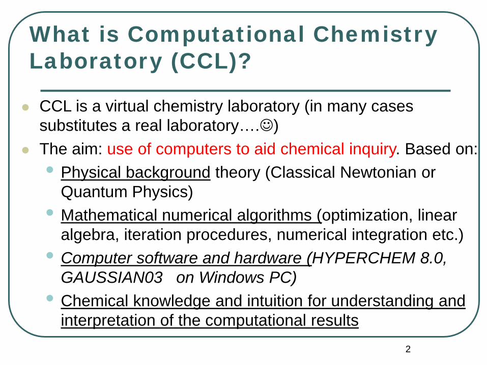
What is Computational Chemistry Laboratory (CCL)?

CCL is a virtual chemistry laboratory (in many cases substitutes a real laboratory….)

The aim: use of computers to aid chemical inquiry. Based on:• Physical background theory (Classical Newtonian or

Quantum Physics)• Mathematical numerical algorithms (optimization, linear

algebra, iteration procedures, numerical integration etc.)• Computer software and hardware (HYPERCHEM 8.0,

GAUSSIAN03 on Windows PC) • Chemical knowledge and intuition for understanding and

interpretation of the computational results

3

Potential Energy Surface (PES) – the main chemistry inquiry“Chemistry – is knowing the energy as a function of nuclear coordinates” F. Jensen

4

Potential energy surfaces (and similar properties) calculation

Classical (Molecular) Mechanics• quick, simple; accuracy depends on parameterization; no

consideration of electrons interaction) Quantum Mechanics:1. Molecular Wave Function Theory

• Ab initio molecular orbital methods...much more demanding computationally, generally more accurate.

• Semi-empirical molecular orbital methods ...computationally less demanding than ab initio, possible on a pc for moderate sized molecules, but generally less accurate than ab initio, especially for energies.

2. Density functional theory… more efficient and often more accurate than Wave Function based approaches.

5

Molecular Mechanics – a theory of molecules “without electrons”

Employs classical (Newtonian) physics

Assumes Hooke’s Law forces between atoms (like a spring between two masses)

Estretch = ks (l - lo)2

graph: C-C; C=O

Force field = {ks,l0}

6

Molecular Mechanics More elaborate Force Fields (FF)

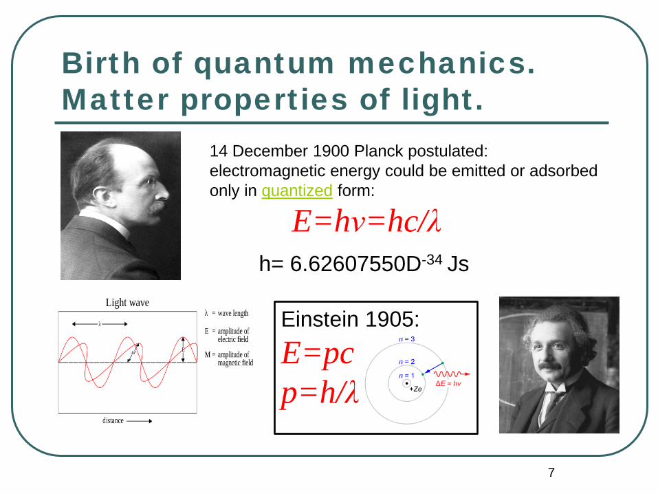
Birth of quantum mechanics. Matter properties of light.

7

14 December 1900 Planck postulated:electromagnetic energy could be emitted or adsorbed only in quantized form:

E=hν=hc/λh= 6.62607550D-34 Js

Einstein 1905:

E=pcp=h/λ

8

Birth of quantum chemistryWave properties of matter

Prince Louis de Broglie (1923):

λ = h/mv= h/ph= 6.62607550D-34 Js

ψp=e-i2πx/λ= e-i2πpx/h

(“wave-particle duality” paradox)

ψ - probabilistic (statistic) wave (Copenhagen interpretation). Waves properties: interference, diffraction etc.

Possible explanation:The probabilistic behavior of elementary particles are connected with structure of quantum vacuum.

9

Basis of Quantum Chemistry

Postulate I : “A closed system is fully described by ψ”• Postulate II: “Operator – for every physical quantity”

(-ih/2π)d/dx (e-i2πpx/h) = p (e-i2πpx/h) (-ih/2π)d/dx (ψp) = p (ψp) Operator – linear and Hermitian

Schrödinger equation (1926):

(can be solved exactly for the Hydrogen atom, but nothing larger)

P.A.M. Dirac, 1929: “The underlying physical laws necessary for the mathematical theory of a large part of physics and the whole of chemistry are thus completely known.”

di H EdtΨ − = Ψ = Ψ

10

One-dimensional Schrödinger wave equation

22

2

22 2

2

2 2

2

2 2

2

ˆ

Total energy kinetic potential12 2

ˆ ˆ ˆ ˆthen

ˆ

ˆ2

2

H E

pmv V Vm

dp i p ppdx

d d dp i idx dx dxdH V

m dxd V E

m dx

ψ ψ

ψ ψ ψ

== +

= + = +

= − =

= − − = −

≡ − +

− + =

Hamiltonian operator• Ĥ = operator of energy• SE = energy eigen-value equation

Extracts total energy, E Many solutions E0, E1, … En

Ψ(x) − wavefunction• No direct physical meaning

|Ψ (x)|2 − Probability of finding particle with energy E at point x• Single-valued, finite, continuous

11

MolecularSchrödinger equation (SE):

Σ 1MA

2A

_ h28π2H = Σ 2

a_ h2

8π2m

electrons

A

>

nuclei

aΣ ZA

rAa_ e2Σ

nuclei electrons

aA

Σ ZAZBrAB

e2Σnuclei

AΣ 1

rabe2Σ

electrons

baB >++

kinetic energy (nuc.) kinetic energy (elect.)

2 kinetic energy terms plus3 Coulombic energy terms:(one attractive, 2 repulsive)

HΨ = EΨ

H = Hamiltonion operator

12

Relativistic quantum mechanicsDirac equation (1928) :

13

Influence of Relativity on Quantum World and vice-versa

(x)

(x) ( )

(x)

(x)

L

L

S

S

x

α

β

α

β

Ψ

Ψ Ψ =

Ψ Ψ

REALITY IS RELATIVISTIC AND THUS IS QUANTUM (and vice-versa!)

14

Dirac’s sea of electrons.Quantum vacuum.

15

The NR molecular wavefunction – physical meaning

The wavefunction, Ψ , is a key quantity in quantum chemistry.

Ψ depends on coordinates and spins. Spin of electron – relativistic property, additional “discrete” coordinate ; |ms1 |=1/2

In a three dimensional system of n-electrons,

is the probability of simultaneously finding electron 1 with spin ms1 in the volume dx1dy1dz1 at (x1,y1,z1), electron 2 with spin ms2 in the volume dx2dy2dz2 at (x2,y2,z2) and so on

The wave function should be normalized, that is, the probability of finding all electrons somewhere in space equals 1.

( ) 21 1 1 1 1,..., , ,..., ....n s sn n n nx z m m dx dy dz dx dy dzψ

( ) 21 1 1 1 1 1

... , , ,..., , , ... 1n n n n n n

all mx y z x y z dx dy dz dx dy dzψ

∞ ∞ ∞ ∞ ∞

−∞ −∞ −∞ −∞ −∞

⋅ ⋅ =∑ ∫ ∫ ∫ ∫ ∫

16

Wavefunction’s general properties The wave function should be antisymmetric, that is, Ψ should

change sign when two electrons of the molecule interchange:

We can use the molecular wavefunction to calculate any property of the molecular system. The average value, <C>, of a physical property of our molecular system is:

where, Ĉ, is the quantum mechanical operator of the physical property and

*ˆ ˆ ˆC C d Cψ ψ τ ψ ψ= ≡∫

1 1 1

... ... n n nall m

dx dy dz dx dy dz dτ∞ ∞ ∞ ∞

−∞ −∞ −∞ −∞

⋅ ⋅ =∑ ∫ ∫ ∫ ∫ ∫

( )( )

1 1 1 ,..., 1

1 1 1 1

, , ,..., , , , , ,..., , , , ,...,

, , ,..., , , ,..., , , ,..., , , , ,...,

i i i j j j n n n s sn

j j j i i i n n n s sn

x y z x y z x y z x y z m m

x y z x y z x y z x y z m m

ψ

ψ

=

−

17

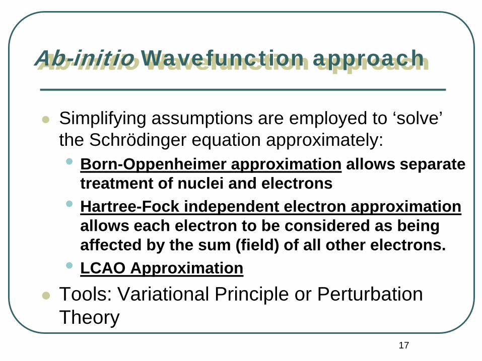
Ab-initio Wavefunction approach

Simplifying assumptions are employed to ‘solve’ the Schrödinger equation approximately:• Born-Oppenheimer approximation allows separate

treatment of nuclei and electrons• Hartree-Fock independent electron approximation

allows each electron to be considered as being affected by the sum (field) of all other electrons.

• LCAO Approximation Tools: Variational Principle or Perturbation

Theory

18

Born-Oppenheimer Approximation -

Σ 1MA

2A

_ h28π2H = Σ 2

a_ h2

8π2m

electrons

A

>

nuclei

aΣ ZA

rAa_ e2Σ

nuclei electrons

aA

Σ ZAZBrAB

e2Σnuclei

AΣ 1

rabe2Σ

electrons

baB >++

kinetic energy (nuc.) kinetic energy (elect.)

1 kinetic energy term plus2 Coulombic energy terms:(one attractive, 1 repulsive)plus a constant for nuclei

constant

19

Steps of solution of the Schrödingerequation in the Born-Oppenheimer approximation:

Htot = (Tn + Vn ) + Te + Vne + Ve= (Hn) + He

1. Electronic SE: He Ψe (r,R)=Ee(R) Ψe (r,R)2. Nuclear SE: (Tn + Vn + Ee(R) )Ωn(R)=En Ωn(R)

Vn + Ee(R) = potential energy surface (PES) TOTAL WF : Φ(r,R) = Ωn(R) Ψe (r,R)In our laboratory we concentrate mainly on solution of the electronic SE and working with PES (finding minimums, transition states etc.)

20

Solving the Electronic SE: Hartree-Fock (HF) approximation –the physical background Multi-electronic SE: He Ψe (r,R)=Ee(R) Ψe (r,R) is still very

complicated → reduce it to the single-electronic equation HF assumes that each electron experiences all the others

only as a whole (field of charge) rather than individual electron-electron interactions.

Instead of multielectronic Shrödinger equation introduces a one-electronic Fock operator F:

F φ = ε φwhich is the sum of the kinetic energy of an electron, a potential that one electron would experience for a fixed nucleus, and an average of the effects of the other electrons.

21

Mathematical foundation of the HF (or Self-consistent-field (SCF)) method

Molecular orbital theory approximates the molecular wave function Ψ as a antisymmetrized product of orthonormal one-electron functions (or “molecular spin-orbitals”)

where  is the antisymmetrization operator and

where k=±1/2; σ1/2 =α ; σ-1/2 =β . The antisymmetrization operator is defined as the operator that

antisymmetrizes a product of n one-electron functions and multiplies them by normalization factor (n!)-1/2

1 2ˆ ( .... )nA f f fψ = × × ×

( , , )i i i i i kf x y zφ σ=

22

Determinant of Slater

The antisymmetrized WF can be represented as the Slater’s determinant:

( )

1 1 1 1 2 1 2 1 / 2 1

1/ 2 1 2 1 2 2 2 2 2 / 2 2

1 1 2 2 / 2

( ) (1) ( ) (1) ( ) (1) ( ) (1) ... ( ) (1)( ) (2) ( ) (2) ( ) (2) ( ) (2) ... ( ) (2)

!... ...

( ) ( ) ( ) ( ) ( ) ( ) ( ) ( ) . . . ( ) ( )

n

n

n n n n n n

x x x x xx x x x x

n

x n x n x n x n x n

φ α φ β φ α φ β φ βφ α φ β φ α φ β φ β

φ α φ β φ α φ β φ β

−Ψ =

23

Variational Principle

The energy E calculated from any approximation of the wavefunction Φ will be higher than the true energy E0:

The better the wavefunction, the lower the energy (the more closely it approximates reality).

Changes (variation of parameters in Φ) are made systematically to minimize the calculated energy.

At the energy minimum (which approximates the true energy of the system), dE/dφi = 0.

*0

ˆE H d Eτ= Φ Φ ≥∫

24

The Hartree-Fock energy functional

We shall restrict ourselves to closed shell configurations, for

such cases, a single Slater determinant is sufficient to describe

the molecular wave function. Using the variational principle

within this framework lead to the restricted HF theory. The

Hartree-Fock energy for molecules with only closed shells is/ 2 / 2 / 2

1 1 1

12 (2 )2

n n ncore

HF i ij iji i j

E H J K= = =

= + −∑ ∑∑21 1

1ˆ(1) (1) (1) (1) / (1)2

core corei i i i I I i

IH H Z rφ φ φ φ≡ = − ∇ − ∑

12 12(1) (2) 1/ (1) (2) , (1) (2) 1/ (1) (2)ij i j i j ij i j j iJ r K rφ φ φ φ φ φ φ φ≡ ≡

25

The Hartree-Fock equations

The Hartree-Fock equations are derived from the variational principle, which looks for those orbitals φ that minimize EHF.

For computational convenience the molecular orbitals are taken to be orthonormal:

The orthogonal Hartree-Fock molecular orbitals satisfy the single-electronic equations:

(1) | (1) i j ijφ φ δ=

ˆ (1) (1) (1)i i iF φ ε φ=

26

The (Hartree-) Fock operator Single-electronic operator:

The Coulomb operator Jj and the exchange operator Kj are defined by

where f is an arbitrary function

/ 221 1

1

1ˆ ˆ ˆ(1) / 2 (1) (1)2

n

I I j jI j

F Z r J K=

= − ∇ − + − ∑ ∑

2

212

*

212

1ˆ (1) (1) (1) (2)

(2) (2)ˆ (1) (1) (1)

j j

jj j

J f f dvr

fK f dv

r

φ

φφ

=

=

∫

∫

27

Next step: MO-LCAO Approximation

Electron positions in molecular orbitals can be approximated by a Linear Combination of Atomic Orbitals (LCAO).

This reduces the problem of finding the best functional form for the molecular orbitals to the much simpler one of optimizing a set of coefficients (cn) in a linear equation:

•φ = c1 χ1 + c2 χ 2 + c3 χ 3 + c4 χ 4 + …• where φ is the molecular orbital (MO) wavefunction

and χ n represent atomic orbital (AO) wavefunctions.

28

One step more:Basis sets (BS)

A basis set is a set of analytical functions (ξk) used to represent the shapes of atomic orbitals χ n:

General contracted BS: χ n=Σk bk(n) ξk(n) Contraction coefficients are calculated in a separate

atomic HF calculation; if k=1 basis set is called uncontracted.

Basis sets in common use have a simple mathematical form for representing the radial distribution of electron density.

Most commonly used are Gaussian basis sets, which approximate the better, but more numerically complicated Slater-Type orbitals (STO).

29

Hartree-Fock Self-Consistent Field (SCF) Method.

Computational methodology (Jacobi iterations):1. Guess the orbital occupation (position) of an electron

(set of MO coefficients {cn })2. Calculate the potential each electron would experience

from all other electrons (Fock operator F ({cn }))3. Solve for Fock equations to generate a new, improved

guess at the positions of the electrons (new {cn })4. Repeat above two steps until the wavefunction for the

electrons is consistent with the field that it and the other electrons produce (SCF).

30

Types of HF Multiplicity (M) = 2*S+1

(S is the total spin of the system) Electrons can have spin up or down . Most

calculations are closed shell calculations (M=1), using doubly occupied orbitals, holding two electrons of opposite spins. RHF – restricted HF

Open shell systems (M>1) are calculated by1. ROHF – restricted open shell HF – the same

spatial orbitals for different spin-orbitals from the valence pair;

2. UHF – unrestricted HF – different spatial parts for different spins from the same valence pair

31

Illustrating an RHF singlet, and ROHF and UHF doublet states

32

Semi-empirical MO Calculations:Further Simplifications of HF

Neglect core (1s) electrons; replace integral for Hcore by an empirical or calculated parameter

Neglect various other interactions between electrons on adjacent atoms: CNDO, INDO, MINDO/3, MNDO, etc.

Add parameters so as to make the simplified calculation give results in agreement with observables (atomic spectra or molecular properties).

/ 2 / 2 / 2

1 1 1

12 (2 )2

n n ncore

HF ii ij iji i j

E H J K= = =

= + −∑ ∑∑21 1

1ˆ(1) (1) (1) (1) / (1)2

core coreii i i i I I i

IH H Z rφ φ φ φ≡ = − ∇ − ∑

12 12(1) (2) 1/ (1) (2) , (1) (2) 1/ (1) (2)ij i j i j ij i j j iJ r K rφ φ φ φ φ φ φ φ≡ ≡

33

Beyond the SCF.Correlated Methods (CM)

Include more explicit interaction of electrons than HF : Ecorr = E - EHF , where EΨ = H Ψ

Most CMs begin with HF wavefunction, then incorporate varying amounts of electron-electron interaction by mixing in excited state determinants with ground state HF determinant

The limit of infinite basis set & complete electron correlation is the exact solution of Schrödinger equation (which is still an approximation)

34

Beyond the SCF.Correlation effects on properties.

35

Two alternative ways of the electron correlation treatment

HF (Hartree-Fock) – “a singe determinant” theory• no correlation included!

1. WF based “multi-determinant” correlation methods:1. Configuration Interaction (CI)

• Variational; CISD, CSID(T) …2. Many-body perturbation theory (including coupled cluster)

• Non-variational; MBPT2, MBPT3; CCSD; CCSD(T)2. Density functional theory (DFT) – correlation method not based on

wave-function, but rather on modification of the energy functional:

Kohn-Sham: A “single determinant” theory including correlation!

/ 2 / 2 / 2

1 1 12 ( )

n n ncore Exch Corr

DFT i ij iji i j

E H J X +

= = =

= + +∑ ∑∑

36

Summary of Choices:

6-311++G**

6-311G**

6-311G*

3-21G*

3-21G

STO-3G

STO

HF CI QCISD QCISDT MP2 MP3 MP4 correlation

increasing size ofbasis set

increasing level of theory

Schrodinger

increasing accuracy,increasing cpu time

infinite basis set

full e-

37

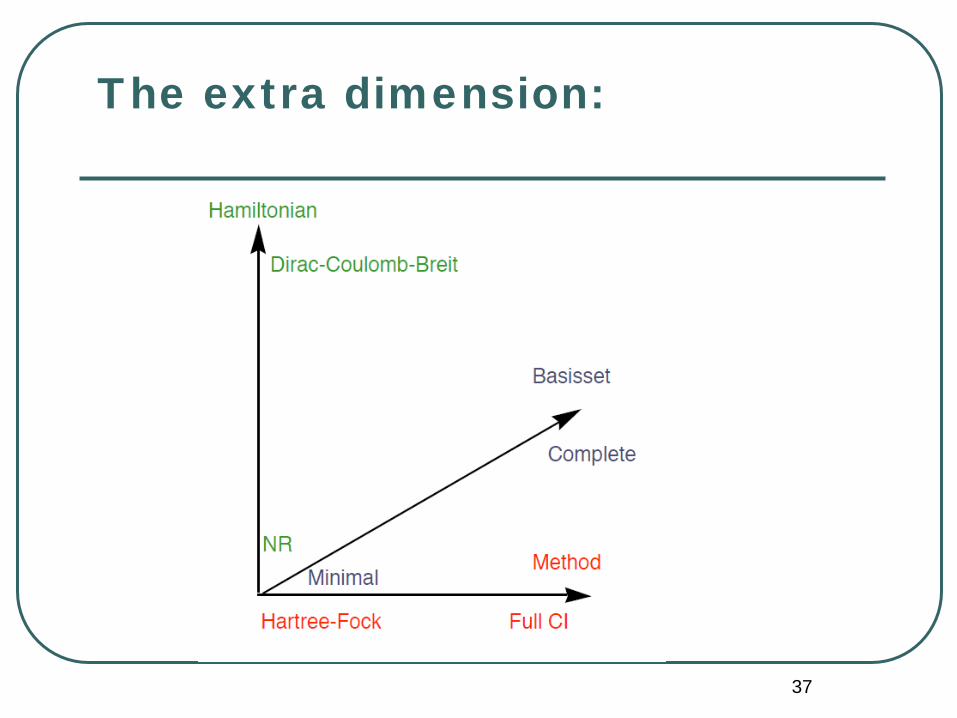
The extra dimension:

38

Summary: Levels of QM Theory

HΨ=EΨ

Born-Oppenheimer approximation

Single determinant SCF

Semi-empirical methods

Correlation approaches:1.Multi-determinantial (MCSCF, CI, CC, MBPT)2. Single determinantial (DFT)

39

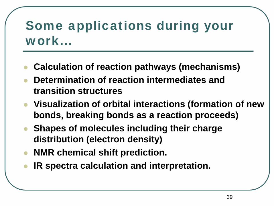
Some applications during your work...

Calculation of reaction pathways (mechanisms) Determination of reaction intermediates and

transition structures Visualization of orbital interactions (formation of new

bonds, breaking bonds as a reaction proceeds) Shapes of molecules including their charge

distribution (electron density) NMR chemical shift prediction. IR spectra calculation and interpretation.

40

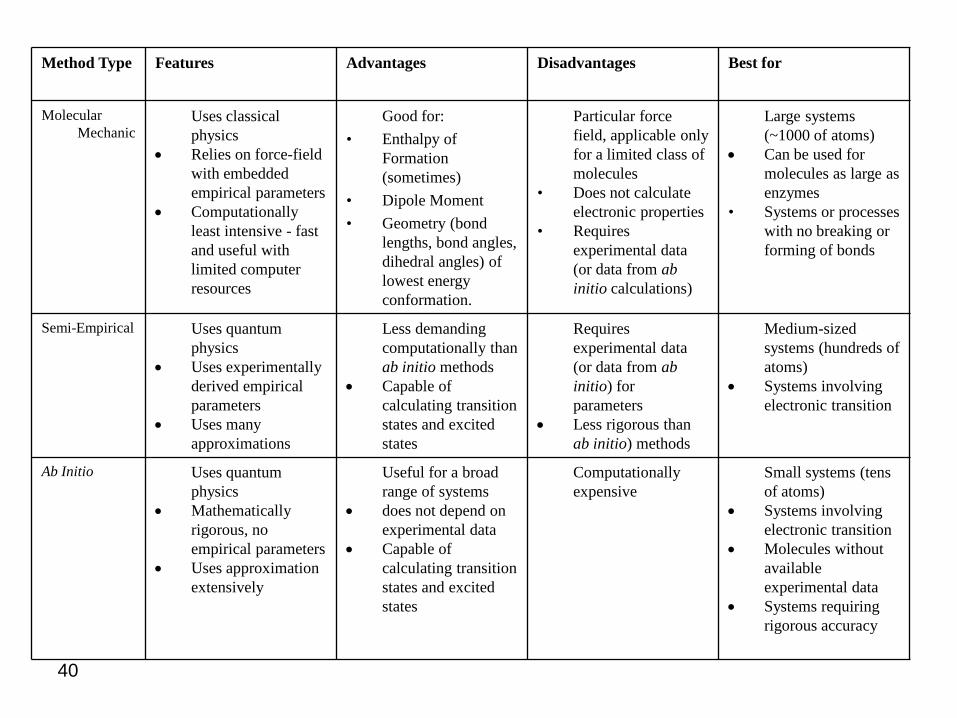
Method Type Features Advantages Disadvantages Best for

Molecular Mechanic

• Uses classical physics

• Relies on force-field with embedded empirical parameters

• Computationally least intensive - fast and useful with limited computer resources

• Good for:• Enthalpy of

Formation (sometimes)

• Dipole Moment • Geometry (bond

lengths, bond angles, dihedral angles) of lowest energy conformation.

• Particular force field, applicable only for a limited class of molecules

• Does not calculate electronic properties

• Requires experimental data (or data from ab initio calculations)

• Large systems (~1000 of atoms)

• Can be used for molecules as large as enzymes

• Systems or processes with no breaking or forming of bonds

Semi-Empirical • Uses quantum physics

• Uses experimentally derived empirical parameters

• Uses many approximations

• Less demanding computationally than ab initio methods

• Capable of calculating transition states and excited states

• Requires experimental data (or data from ab initio) for parameters

• Less rigorous than ab initio) methods

• Medium-sized systems (hundreds of atoms)

• Systems involving electronic transition

Ab Initio • Uses quantum physics

• Mathematically rigorous, no empirical parameters

• Uses approximation extensively

• Useful for a broad range of systems

• does not depend on experimental data

• Capable of calculating transition states and excited states

• Computationally expensive

• Small systems (tens of atoms)

• Systems involving electronic transition

• Molecules without available experimental data

• Systems requiring rigorous accuracy