Semi-Automatic Floating-Point Implementationof Special FunctionsChristoph Lauter* and Marc Mezzarobba*†

*Sorbonne Universités, UPMC Univ Paris 06, UMR 7606, LIP6, F-75005, Paris, France†CNRS, UMR 7606, LIP6, F-75005, Paris, France

christoph.lauter@lip6.fr, marc@mezzarobba.net

Abstract—This work introduces an approach to the computer-assisted implementation of mathematical functions geared towardspecial functions such as those occurring in mathematical physics.The general idea is to start with an exact symbolic representationof a function and automate as much as possible of the processof implementing it.

In order to deal with a large class of special functions, oursymbolic representation is an implicit one: the input is a lineardifferential equation with polynomial coefficients along withinitial values. The output is a C program to evaluate the solutionof the equation using domain splitting, argument reduction andpolynomial approximations in double-precision arithmetic, in theusual style of mathematical libraries.

Our generation method combines symbolic-numeric manipu-lations of linear ODEs with interval-based tools for the floating-point implementation of “black-box” functions. We describea prototype code generator that can automatically produceimplementations on moderately large intervals. Implementationson the whole real line are possible in some cases but requiremanual tool setup and code integration. Due to this limitationand as some heuristics remain, we refer to our method as “semi-automatic” at this stage.

Along with other examples, we present an implementationof the Voigt profile with fixed parameters that may be ofindependent interest.

I. Introduction

Fixed-precision floating-point (“FP”) operations come withvarying performance and accuracy guarantees. Basic operationssuch as multiplication are typically implemented in hardwareand, being correctly rounded, provide perfect accuracy. So-called elementary functions like exp and log are providedin software through general-purpose mathematical libraries(libms). They are well-optimized for performance and eithercorrectly rounded, as recommended by the IEEE754 Stan-dard [16], or provided with maximum error not exceeding oneunit in the last place.

This work is concerned with special functions, i.e., “functionswhich are widely used in scientific and technical applications,and of which many useful properties are known” [12]. Some,like Bessel functions or the Gaussian error function, are presentin some libms. Most are provided by specialized librariessuch as GSL or Root. Others are only available in computeralgebra systems like Maple and Pari and have no efficientfixed-precision implementation. The NIST Digital Libraryof Mathematical Functions [1] contains a good overview ofexisting implementations.

There is a huge gap in both performance and rigor betweenthese implementations and state-of-the-art elementary functions.However, implementing or reimplementing special functionsmanually in the classical way is tedious and requires consider-able expertise. And indeed, in many cases, publicly availableimplementations of a given special function all derive from asingle source, typically Cephes [23].

This article presents the first results of a project exploringthe implementation of special functions through automaticcode generation. In our view, this is the only feasible way toimplement wider classes of special functions while bridgingthe quality gap with respect to elementary functions. Addi-tionally, code generation allows for production of specializedimplementations taylored to specific applications, in terms ofaccuracy, supported domain or code properties.

Our focus is on special functions satisfying linear ordinarydifferential equations of the form

pr(x) f (r)(x)+· · ·+p1(x) f ′(x)+p0(x) f (x) = 0, pi ∈ Q[x]. (1)

Such functions are called D-finite or holonomic. A key ideain the field of D-finite functions is that an equation suchas (1) along with initial values makes up a concise exactrepresentation of its solution that can be used in computations.

Many common special functions can be defined this way.Among the better known special functions of mathematicalphysics, univariate D-finite functions include in particular theerror function (and related functions such as the Dawsonfunctions or the Voigt profile), the Airy functions (as wellas Scorer functions, generalized Airy functions. . . ), the Besseland Hankel functions, the Struve functions of integer order,the hypergeometric and generalized hypergeometric functions,the spheroidal wave functions, and the Heun functions.

Under the term code generator, we understand a softwaretool which takes as input a description of a function f , a setof floating-point inputs X and a target accuracy ε > 0, andwhich generates source code (in our case, in C) that providesa function f satisfying

∀ x ∈ X,

f (x) − f (x)

f (x)

≤ ε. (2)

In this work, we consider inputs in IEEE754 double precision(binary64) format taken in a relatively small interval [a, b],say of width b − a < 100, and accuracies compatible with thatformat, i.e., 2−53 ≤ ε ≤ 1. These restrictions can be loosened

with some manual work so that implementations on the wholeset of double precision numbers become feasible.

Code generation for mathematical functions is not entirely anew idea. A powerful toolbox, including in particular Gappa [8]and Sollya [6], has been developed in recent years to helphuman developers with the most tedious steps of the imple-mentation process. Building on these advances, several authorshave considered code generation both for “flavors” of a fixedfunction and for “black-box” functions given as executablecode [19], [9], [3], [18], [4]. Independently, Beebe [2] pro-duced a new, very extensive mathematical library with the helpof semi-automatic code generation. We base our work on theblack-box approach of [19], where the starting point is exe-cutable code able to evaluate f and its first few derivativeson intervals, up to any required precision. Providing such anevaluator is easy when f is a composition of basic elementaryfunctions, thanks to multiple-precision interval libraries, but itis a major limitation for more general functions.

Nevertheless, if f satisfies some kind of functional equation,any rigorous arbitrary-precision numerical solver could in prin-ciple play the rôle of the black box. In the case of D-finitefunctions, such solvers can be built in practice [25], [31]. More-over, the behavior of D-finite functions in the neighborhoodof their singularities is well-understood, opening the door tofurther extensions of the method. These observations were, insome sense, the starting point of the present work. We soonobserved that the interval black-box model it is not well suitedto our case, as the number of queries to the function tends tobe very large. This led us to favor a different interface, basedon polynomial approximations, as described in Section II.

This article is organized as follows. Section II describes thegeneral architecture of our function generation pipeline andintroduces our prototype implementation. Section III focuses onthe frontend part, that is, the rigorous ODE solver. Section IVdiscusses the backend, which is the part in charge of floating-point implementation choices. The remaining section presentsexperimental results and applications.

II. Overall architecture

This text describes both an approach to code generationfor D-finite functions and experiments performed with aprototype implementation of this approach. Our prototype,named Frankenstein, is available from https://gforge.inria.fr/git/metalibm/frankenstein.git. It is based on modified versionsof two existing software packages, Metalibm [18], written inSollya [6], and NumGfun [21], written in Maple. The nameshould give a pretty accurate idea of how the combination isrealized. Thus, not all design choices have the same signifi-cance: while some would survive a cleaner rewrite, others areonly justified by the goal of producing a usable prototype outof two research-quality codes that had never been intended towork with each other. Here we focus on the former category,with brief mentions of more peculiar features of Frankensteinas necessary.

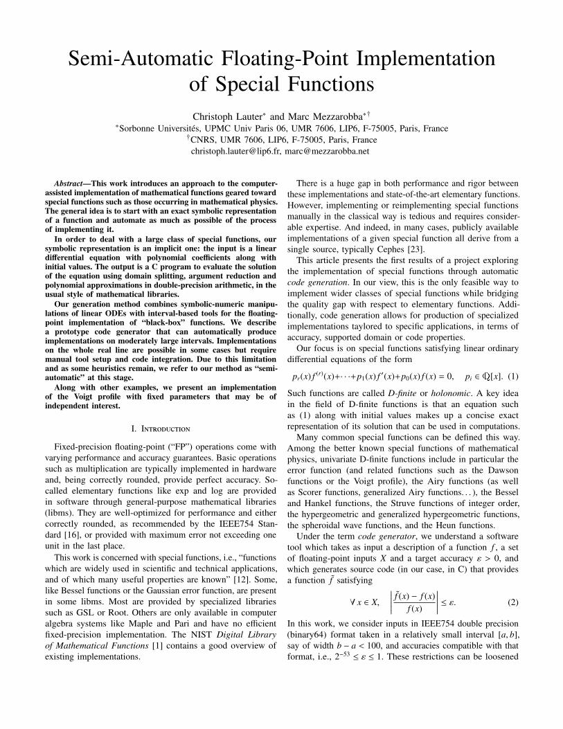
Consider a sufficiently small interval I = [a, b] ⊂ R anda solution f of (1) defined on I. Assume for simplicity that

differential equation

truncated Taylor series

compact rough approx.

tight approximation

representable approximation

implemented polynomial

C code

bounds, recurrence

economization

Remez algorithm,domain splitting

FP coeff. optim.

error-free transf.,FP error analysis

Frontend

Backend

Figure 1. A piecewise polynomial approximation pipeline.

0 ∈ I and pr(x) , 0 for x ∈ I. The function f is then analyticon I, and the vector of initial values F(0) = ( f (0), . . . , f (r−1)(0))characterizes f among the solutions of (1). Assume additionallythat | f (x)| ≤ 21024(1 − 2−53) for x ∈ I. Then, special floating-point values (NaN, ±∞) occur neither on input nor on output.Denoting by F the set of double-precision numbers, our goal isto produce a program computing a value f (x) ∈ F satisfying (2)with X = I ∩ F.

Our method takes as input (pi)ri=0 and F(0) (which together

define f ), I, ε, and various constraints on allowable implemen-tations. It either succeeds and produces a program satisfying (2)by construction1, or fails if no implementation fitting the con-straints is found. Failure does not imply that no feasible solutionexists.

One way to view the process leading from the definitionof f by (1) to an implementation is as a rigorous piecewisepolynomial approximation pipeline, as illustrated on Figure 1.Each stage receives a set of approximations of f (and possiblyits first few derivatives) by polynomials on subintervals of Iand produces approximations with different properties that arepassed on to subsequent stages. The subintervals vary fromstage to stage, and typically overlap even within a single stage.For example, the domain splitting procedure can use both arough approximation on the whole domain to get a generalpicture of the behavior of f , and tight approximations on tinyintervals to compute precise values.

The complete pipeline can be approximately divided into afrontend and a backend. Roughly speaking, the frontend is the

1This is not entirely true of Frankenstein yet. Although the overwhelmingpart of the code uses rigorous error bounds, some heuristic estimates remain.

part where decisions are driven by the analytic properties of f .The backend is the part where they are driven by the floating-point environment and other implementation constraints. Towork with another class of mathematical functions, one wouldreplace the frontend; to target a different evaluation environment(fixed-point arithmetic, say), one would swap out the backend.There is no formal abstraction of how the backend can querythe function, though, and both parts have full knowledge ofthe implementation problem.

In Frankenstein, the frontend and the backend respectivelycorrepond to NumGfun and Metalibm. For convenience reasons,the process is driven by the backend, which can ask the frontendfor approximations of variable quality on various subintervals.As we reuse code written for the black-box function model, thebackend mostly uses these approximations to perform intervalevaluations, but we expect to make more direct use of thepolynomial representation in future developments.

Our general implementation strategy fits the standard patternof special function implementations and is especially close tothat of Harrison [14]. Classical argument reduction algorithmsbased on algebraic properties of elementary functions typicallydo not apply. Accordingly, the only feature of f that we con-sider to reduce the implementation domain is its parity. Parityproperties can be detected either by numerical comparison off (x) and f (−x) (as Frankenstein currently does), or based onthe differential equation. Periodic functions could be handledin a similar way but are very uncommon.

We then single out a small number of “interesting points”,the neighborhood of which need to be handled in a specialway. Under our working hypotheses, interesting points includex = 0, where the floating-point grid is denser than usual, andthe points x with f (x) ≃ 0, where obtaining a relative errorbound requires special care. In a more general setting, onewould add at least ±∞ and the singularities of f to the list. Ina small interval around each interesting point, approximationsof f are computed and implemented in a way that takes intoaccount the special constraints. The remaining subintervals (ifany) are further subdivided until approximation by small-degreepolynomials becomes feasible.

Let us now consider in more detail the main ingredients ofthe process, starting with the frontend.

III. From a differential equation to rigorous approximations

The frontend’s rôle is to provide the backend with rigorouspolynomial approximations of f of the form

∀x ∈ J, | f (x) − p(x)| ≤ η (3)

for various subintervals J ⊆ I. As Equation (3) suggests, inour architecture, the approximations come with absolute errorbounds. Indeed, these are often easier to obtain and this choicedoes not hinder the use of relative error bounds in later stages.

Values of J above can range from point intervals J = {x}to J = I. It is not necessary that the frontend be able to findapproximations on arbitrarily wide intervals, as the backendhas the necessary logic to split J if the returned error bound isinfinite (or too large). The only requirement is that sufficiently

precise queries on sufficiently thin intervals eventually producesatisfying approximations.

The smallest useful value of η in our setting is slightly lessthan the smallest subnormal number, 2−1074. In principle, itwould be possible to replace f once and for all by a set ofpolynomial approximations achieving such an accuracy. Thefrontend of Frankenstein is more flexible and can computearbitrarily good approximations. Precise polynomial approx-imations on wide intervals quickly become large and costlyto compute. For historical reasons, our frontend provides aseparate interface dedicated to points and very thin intervalsthat always returns “polynomial approximations” reduced toconstants, which can reach absolute precisions log η−1 in thehundred of thousands if necessary.

The computation of the approximations (3) is based on acombination of classical techniques that we now summarize.We refer the reader to [31], [21] for details.

A. Transition matrices

Recall that f is specified by the differential equation (1) andthe vector of initial values F(0), or, to be precise, rigorous arbi-trary precision approximations of F(0). Let us also extend thenotation F(x) = ( f (x), . . . , f (r−1)(x)) to arbitrary x. Polynomialapproximations on an interval J ⊆ I will be derived from theTaylor expansion of f around the center c of J. This expan-sion is easily computed from the differential equation and the“initial value” F(c). To deduce F(c) from F(0), we use Taylorexpansions at intermediate points x0 = 0, x1, . . . , xn = c chosenin such a way that xk+1 lies within the disk of convergence ofthe Taylor expansion of F at xk. In other words, our frontendis essentially a rigorous ODE solver based on the so-calledmethod of Taylor series [20].

More precisely, we proceed as follows [7], [31]. By linearityof (1), for all x, y ∈ I, there exists a matrix ∆x(y) ∈ Rr×r

depending only on (1) (not on the particular solution f ) andsuch that F(y) = ∆x(y) F(x). We have ∆x(z) = ∆y(z) ∆x(y) forall x, y, z, and hence

F(c) = ∆0(c)F(0) = ∆xn−1 (c) . . .∆x1 (x2) ∆0(x1) F(0). (4)

The entries of ∆x(y) are values at y of solutions of (1) cor-responding to unit initial values at x (or derivatives thereof).Denoting by ρ(x) the distance from x to the nearest complexroot of the leading coefficient pr of (1), the Taylor expan-sion at x of any solution of (1) has radius of convergence atleast ρ(x). It is a classical fact that the coefficients of these ex-pansions obey linear recurrences with polynomial coefficients,making it easy to compute as many terms as needed. As we as-sumed that pr does not vanish on I, computing F(c) reduces toforming the product (4), where each factor ∆x(y) can be evalu-ated by summing convergent power series whose coefficientsare easy to compute. Binary splitting can be used to computethe partial sums efficiently to very high precisions [7].

Our assumption that the initial values are provided at a pointof I is artificial: the above argument still works with 0 < Ias long as the leading coefficient pr(x) of (1) does not vanishbetween 0 and I. In addition, (1) actually defines f for complex

values of x, and nothing prevents the path (x0, . . . , xn) fromgoing through the complex plane. If pr(s) = 0 for some sbetween 0 and I, analytic continuation along a path avoiding sstill defines f on I (in general in a way that depends on thepath). Furthermore, when 0 < I, we can relax the assumptionthat pr(0) , 0: the theory extends to the case where 0 is aso-called regular singular point of (1) [32], [21]. Both of theseextensions are supported in Frankenstein, albeit with specifictool setup and subject to heuristic error estimates in somecases. The second one is useful because many classical specialfunctions are best characterized by their behavior at regularsingular points of their defining equation. A typical exampleis the family of Bessel functions (see Example 3 below).

B. Error bounds

It is crucial that the frontend provides rigorous error boundson the approximations it computes, as these approximationsare the backend’s only access to the function f . Here, werecall a simple bound computation technique based on thetheory of majorizing series [15, Chap. 2]. Frankenstein (viaNumGfun) actually uses a more sophisticated variant of thesame technique [22], but the present version conveys the mainideas and would probably suffice for our purposes.

Consider a power series with matrix coefficients (or, equiva-lently, a matrix of power series) Y(x) =

∑∞n=0 Ynxn ∈ Rr×r[[x]],

and let ‖ · ‖ denote a matrix norm. We write Y 4 w ifw(x) =

∑∞n=0 wnxn ∈ R+[[x]] is a power series that bounds Y

coefficient-wise, i.e., ‖Yn‖ ≤ wn for all n ∈ N. The method trans-fers such bounds on the coefficients of differential equationsto similar bounds on the solutions.

Our goal is to control the error committed by truncatingthe Taylor expansions of a solution of (1). Without loss ofgenerality, we restrict ourselves to Taylor expansions at theorigin. Rewrite (1) in matrix form, as

Y ′(x) = P(x)Y(x), (5)

where P ∈ Q(x)r×r is a companion matrix with entries of theform p(x)/pr(x), and for notational simplicity Y is also takento be a matrix. The matrix function P admits a convergentpower series expansion at 0, whose coefficients Pn satisfy||Pn|| = O(αn) for all α > ρ(0)−1. Given such an α, it is not toohard to compute M > 0 such that

P(x) 4 q(x) :=αM

(1 − αx).

Expanding both sides of (5) in power series and collecting thematching powers of x, we obtain

(n + 1)Yn =

n∑j=0

PnYn− j. (6)

The same reasoning applied to the equation w′(x) = q(x)w(x)yields

(n + 1)wn =

n∑j=0

qnwn− j. (7)

Now assume w0 > ‖Y0‖. Comparing (6) with (7), we see byinduction that Y(x) 4 w(x). But the second equation is solvablein closed form: we have

w(x) =w0

(1 − αx)M .

This explicit expression makes it easy to bound the tails wnxn +

wn+1xn+1 + · · · , and hence also Ynxn + Yn+1xn+1 + · · · , whichyields truncation orders that guarantee a certain accuracy.

C. Polynomial approximations

We are now ready to combine the results of the previoussections to obtain rigorous polynomial approximations on agiven interval J. Write J = [c − δ, c + δ], and assume thatδ < ρ(c). With the notation of Section III-A, we have

F(c + ξ) = ∆c(c + ξ) ∆xn−1 (c) . . .∆x1 (x2) ∆0(x1) F(0) (8)

for |ξ| ≤ δ. Each factor (except F(0)) is given by power seriesthat we can truncate so as to guarantee a prescribed accuracy.Error bounds on the individual factors are combined by repeateduse of the inequality

‖AB − AB‖ ≤ ‖A‖ ‖B − B‖ + ‖A − A‖ ‖B‖.

Once we replace each series by a truncation (and F(0) by anapproximation with rational entries), the entries of (8) becomepolynomials in ξ with rational coefficients.

Thus, we compute the entries of ∆c(c + ξ) truncated to asuitable order as polynomials in ξ and multiply the resultingmatrix by an approximation of ∆0(c) F(0). The entries of theresult readily provide the first r derivatives of f . Higher-orderderivatives, if needed, can be obtained by multiplying F(c + ξ)on the left by a row vector of rational functions (or polynomialapproximations of rational functions) deduced from (1). InFrankenstein, most of these steps are performed exactly, usingmultiple precision rational arithmetic. Roundoff errors in theremaining steps are taken into account in the result.

Taylor series typically do not provide good approximationson intervals. Additionally, the bounds of Section III-B can bequite pessimistic. For these reasons, polynomials computed asoutlined above tend to have very high degree. However, dueto the way they are constructed, the rescaled coefficients cnδ

n

quickly decrease to zero, and typically |cn ξn| ≪ η for large n.

Before handing it to the backend, the frontend hence reducesthe degree of the computed polynomial p by economization [11,§4.6]: while the leading term of p is small compared to η,a multiple of the Chebyshev polynomial Tn (rescaled to theinterval J) chosen so that the leading terms cancel is subtractedfrom p. The error bound is updated accordingly. (The choiceof Chebyshev polynomials makes it possible to take advantageof the fact that the error bound only needs to hold for x ∈ J,not for complex x with |x − c| < δ.) This procedure is veryeffective at producing polynomials of reasonable size that caneasily be manipulated by the backend.

IV. From rigorous approximations to evaluation code

It is the backend’s job to transform the high-degree, roughapproximation produced by the frontend into fine-tuned approx-imations with suitable FP properties and eventually, into sourcecode. In absence of classical argument reduction techniques,implementation of the function is reduced to piecewise polyno-mial approximation. The backend hence needs to compute fourpieces of information, as discussed in the next subsections.

1) The implementation interval I needs to be split intosubintervals Ik, together covering I, such that an approximationpolynomial of small degree is possible over each Ik.

2) These small degree polynomials need to be computed,initially with real coefficients.

3) Connected with the approximation step is the problem ofchoosing an appropriate translation f (tk + ·) on a new domainIk − tk. Indeed, the evaluation of the approximation behavesbetter when Ik − tk is a small interval around 0.

4) The backend needs to transform the small-degree approx-imation polynomial on each subdomain into a polynomial withFP coefficients, suitable for evaluation in FP arithmetic, andgenerate code for that FP-based polynomial evaluation.

A. Domain splitting

Given a target accuracy ε and a maximum degree d, thebackend starts with computing a list of intervals Ik touchingeach other in so-called split-points sk, i.e. such that Ik−1 ∩ Ik =

{sk}, covering the whole interval I =⋃

k Ik and such that foreach k there exists a polynomial pk ∈ R[x] of degree no largerthan d approximating f on Ik with a relative error at most ε:

∀ k, ∀ x ∈ Ik,

pk(x) − f (x)

f (x)

≤ ε. (9)

Such a splitting can be computed using an algorithm [18] basedon bisection, interpolation of f in Chebyshev nodes and appli-cation of de la Vallée-Poussin’s theorem [5]. In Frankenstein,we leverage the existing Sollya procedure guessdegree [6]to implement this step.

B. Small degree polynomial approximation

On each subdomain Ik, the backend computes a polynomialapproximation pk ∈ R[x] of degree at most d for the function f .The pk are computed as minimax approximations with relativeerror, using a modified Remez-Stiefel algorithm [5]. However,these polynomials with real coefficients2 are not immediatelysuitable to IEEE754 FP evaluation. Several problems arise.

When 0 < Ik, in particular when Ik contains values x ∈Ik that are significantly larger than 1, Horner evaluation (orany other Estrin-like evaluation) may behave badly. Roughlyspeaking, at each step qi+1(x) = ci + x × qi(x), the evaluationerror accumulated on qi(x) will be amplified by multiplicationwith x when |x| ≫ 1, not attenuated [19]. After splitting Ik ifits radius is too large, we translate both the function f and theinterval Ik by tk to always be in the case when all x ∈ Ik − tk

2As the underlying Sollya environment is FP-based, any polynomial we canexhibit has of course FP coefficients. However, as precision may be increasedat will at this generation stage, the polynomials appear to have real coefficients.

stay small. In most cases, taking (a rounded value of) themidpoint of Ik is appropriate, while ensuring that the translatedargument ξ = x − tk can be computed exactly in FP arithmeticthanks to Sterbenz’ lemma [29], [19]. Special care is usedwhen f has a zero in Ik (see Section IV-C). Further, tk may beoptimized to take into account FP effects on the coefficientsof the polynomial [19].

When Ik is small and the function f is symmetrical aroundsome point in Ik, the minimax approximation polynomial pk

tends to reflect the symmetry: some monomials have verysmall coefficients compared to others. This effect may hinderFP Horner evaluation due to catastrophic cancellation but it canalso be exploited to reduce the number of non-zero coefficientsof the polynomial [10].

C. Achieving relative error bounds for functions with zeros

Clearly, the ratio (pk(x) − f (x))/ f (x) can stay bounded onlyif f has no zero in the domain for x ∈ Ik or if pk has a zerowherever f has one. Classical polynomial approximation theoryeither considers absolute error bounds or excludes functionswith zeros. It can be extended to cover approximation withrelative error of functions f with f (0) = 0 as follows: when f isknown to have a zero of multiplicity m at x = 0, one computesa polynomial approximation qk of x−m f (x) and takes pk(x) =

xm · qk(x). The only requirement is not to use Remez’ originalminimax algorithm but an enhanced version by Stiefel [5].

Since the backend anyway uses approximation domains Ik−tkcontaining 0, the technique above already makes it possible tohandle functions with a zero at some FP number. It suffices totake Ik small enough to contain a single zero of f and tk equalto that zero in order to obtain f (tk + ξ) = 0 for ξ = 0. Thevalue of tk, can easily be computed with any numerical solver,such as Newton’s iteration. No rigor is required in this step; ifthe zero is not correctly determined, relative error polynomialapproximation will simply fail.

The technique no longer applies when f has a zero c < F.However, in this case, f is actually never zero on the FP num-bers it is to be evaluated at. This means that even if the ratio(pk(x) − f (x))/ f (x) is unbounded for x ∈ Ik, it stays boundedover Ik ∩ F. Provided that the procedure we use to bound therelative error only takes into account FP numbers, approxi-mation of a function f with non-FP-representable zeros boilsdown to two subproblems: computing a minimax polynomialfor f and translating the original function such that FP-basedpolynomial evaluation will exhibit bounded evaluation error.

The minimax polynomial can be computed as follows: thefunction g(x) = f (c + x) has an exact (FP-representable) zeroat 0, and can be evaluated at any desired precision by com-puting c with a rigorous Newton algorithm. In the Sollyaframework, g is implemented by an expression tree contain-ing a constant function c whose evaluation algorithm searchesthe original domain Ik for a zero of f whenever and at what-ever precision needed. This is enough for the Remez-Stiefelminimax algorithm to be applicable to g.

Once c itself and a polynomial p(x) approximating g(x) overIk − c are known, we set tk to c rounded to the nearest FP

number. The polynomial r(x) = p(tk − c + x) then approximatesf (tk + x) over Ik − tk ∋ 0. At x = tk (the FP value nearestto c), the translated argument ξ = x − tk is exactly zero, henceFP Horner evaluation of r will return the constant coefficientof r, which is equal to (a rounded version of) f (c). For theFP x just after the zero, ξ will fit on a small number of bitsdue to cancellation in ξ = x − tk, hence FP Horner evaluationwill behave correctly, too. The accuracy of evaluation can bechecked statically using Gappa as explained below.

Note, though, that the polynomial r passed to the codegeneration step then contains coefficients involving the Newton-iteration based representation of c. In contrast, in the usual case(when f has no zero in the domain), the coefficients directlycome from the Remez-Stiefel minimax algorithm.

D. FP code generation for polynomials

Finally, the backend needs to generate a code sequence,based on IEEE754 FP arithmetic, for each subdomain Ik, andto connect these code sequences through a branching sequencedetermining the appropriate subdomain given an input x ∈ I.Generating the subdomain determination sequence is easy.

Generating the polynomial evaluation is harder. The backendtakes the following four sub-steps.

1) It determines the minimal precisions needed for the coeffi-cients of the approximation polynomial pk on each subdomain,following the approach described in [19].

2) It replaces the polynomial pk ∈ R[ξ] with a polynomialpk ∈ F[ξ] with FP coefficients. This could be done by roundingthe real coefficients, however, equi-oscillation properties of theminimax polynomial and therefore accuracy might be affectedtoo much. We therefore use a technique [5] based on latticereduction which globally searches for a FP-valued-coefficientspolynomial “close” to the original real-coefficients polynomial.

3) Starting with the target accuracy ε, the backend esti-mates suitable accuracies for the intermediate steps of a Hornerevaluation of pk. This choice of accuracies determines theFP precisions—and, possibly, double-double or triple-doubleexpansions—to be used in the different steps. The technique isdescribed in [10], [19]. The backend then outputs C code forpolynomial evaluation along with a Gappa [8] proof script.

4) Finally, the backends runs the proof script using Gappa,hence verifying the correctness of the accuracy estimates es-tablished in the previous step.

E. Evaluation-based vs. polynomial-based interfaces

In a cleanly designed special function code generator, thebackend would take the rough polynomial approximationsproduced by the frontend and proceed with refining themwithout ever returning back to the original function f . However,this would require the frontend to take into account the relativeerror due to replacing f by a polynomial, which requires someunderstanding of FP properties of the eventual implementationwhen f has zeros in the domain.

For that reason and for reasons due to the reuse of exist-ing code, Frankenstein works in a slightly different way. Thebackend binds a Sollya function object, corresponding to f , to

the evaluator dedicated to tiny intervals provided by the fron-tend. This would in principle be enough for the backend to run,since the backend—in all steps, even its polynomial approxi-mation ones—is purely based on (interval or point) evaluation.In practice, this simple interface is not enough. The number offunction evaluations is too large to allow for reasonable codegeneration performance. In addition, an evaluation-based in-terface makes it hard to capture non-local properties of thefunction f , such as monotonicity.

We therefore enhanced Sollya to allow a function object,such as the one bound to the frontend’s representation for f ,to be annotated with an alternate approximate representationalong with a bound on the approximation error. The approxi-mation polynomials generated by the frontend provide such anapproximate representation. When it needs to evaluate the func-tion f at some point or over some interval, Sollya first tries touse the annotation. If this first try is inconclusive, for instanceif the approximation error is too large in view of the evalua-tion precision, it falls back to the original evaluator bound tothe frontend. Interval evaluation using the annotation exploitsglobal properties of the polynomial. In particular, monotonicityover the whole annotation interval is detected once and for alland later used to reduce interval evaluations on subintervals toevaluations at their endpoints.

That combination has given Frankenstein the necessary per-formance. We should mention however that making the an-notation mechanism usable for our purposes required somefine-tuning in the Sollya architecture. In particular, as we haveseen, the backend manipulates not only f itself, but also expres-sion trees containing compositions of f with other functions,which need to be reflected on any polynomial annotation. Inaddition, code written in the evaluation-based model tends toperform high-precision evaluations with no real need (that is,to request information on f that cannot have any influence onthe correctness of the generated code). The whole benefit ofthe polynomial annotations can be lost if too many evaluationsfall back to a slow arbitrary-precision evaluator that will tryto satisfy these requests.

V. Examples and experiments

A. Bounded intervals

As already mentioned, there is no complete guarantee thatFrankenstein succeeds to implement a given D-finite function.The following experiments show how it performs on classicalspecial functions. All these examples were handled automati-cally, with minimal manual setup. The reported timings weremeasured on a typical desktop computer.

We start with a simple example where the functions staysaway from zero on the whole implementation domain.

Example 1: The complementary error function erfc(x) =

1 − 2π−1/2∫ x

0 e−t2dt can be defined as the solution of

f ′′(x) + 2x f ′(x) = 0, f (0) = 1, f ′(0) = −2/√π.

We implemented erfc in the range I = [−2; 2], with a targetaccuracy ε = 2−62, under the constraint that no generated

-1.2e-19-1e-19-8e-20-6e-20-4e-20-2e-20

02e-204e-206e-208e-201e-19

-2 -1.5 -1 -0.5 0 0.5 1 1.5 2

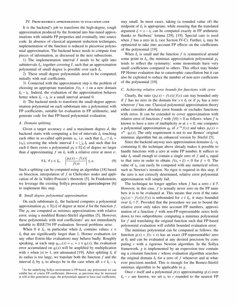
Figure 2. Relative overall error of generated implementation of erfc on [−2; 2].

polynomial have more than 14 non-zero coefficients. Sucha target accuracy slightly beyond double precision is typicalfor first phases of correctly rounded implementations [24],[19]. Though we excluded them above, our code generator isable to handle such accuracies in simple cases, automaticallyintroducing double-double expansions [28], [19] as necessary.

Figure 2 shows a plot of the relative error f (x)/ f (x) − 1 ofthe implementation. Code generation took around 780 seconds.The code generator split I into 16 subdomains of varyinglength. In the subdomain I7 = [−2/3; 2/3], the only nonzerocoefficients of the generated polynomial are those of odd degreeand that of degree 22, taking advantage [10] of an approximatesymmetry around 0. Accordingly, the Horner evaluation codefor x ∈ I7 performs evaluations in x2 in all but one steps.When executed, our implementation takes between 110 and350 machine cycles per call, with most calls completing in 260cycles. For comparison, a call to a typical libm exponentialtakes around 80 cycles.

We then consider an example with several zeros, none ofwhich is representable in floating-point.

Example 2: The Airy function Ai satisfies⎧⎪⎪⎨⎪⎪⎩ Ai′′(x) − x Ai(x) = 0,

Ai(0) = 3−2/3Γ(2/3)−1, Ai′(0) = −3−1/3Γ(1/3)−1.

We implemented Ai on I = [−4.5; 0], asking for an accu-racy ε = 2−45. Frankenstein takes 280 seconds to generate animplementation. It splits the domain into 10 subdomains. Intwo subdomains polynomials with some zero coefficients areused; the generated code precomputes x2 accordingly. It canbe checked that all subdomains containing zeros of Ai(x) aretranslated by an amount equal to the double-precision numbernearest to the zero, and an error plot confirms that the targetaccuracy is met even in the neighborhood of the zeros. Eval-uation of the generated function takes 60 to 90 cycles, withmost calls completing in 72 cycles.

Our last example directly parallels Harrison’s implementationof Bessel functions for “small” arguments [14, Section 3].

Example 3: The Bessel functions J0 and Y0 are defined assolutions of Bessel’s equation

x f ′′(x) + f ′(x) + x f (x) = 0. (10)

We consider the function J0 on the interval I = [0.5; 42] with atarget accuracy of ε = 2−45. The immediate neighborhood of 0

00.05

0.10.15

0.20.25

0.3

-10 -5 0 5 10

Figure 3. V(x) for σ = 1, λ = 12 .

is excluded because (10) is singular at x = 0 (its leading coef-ficient vanishes). For the same reason, initial values f (0), f ′(0)do not make sense for an arbitrary solution of (10). However,J0 can still be defined as the unique solution whose value tendsto 1 as x→ 0. As mentioned in Section III-A, Frankenstein’sfrontend supports such generalized initial conditions.

Code generation starting from this specification took about33 minutes. The code generator splits the domain I into 18subdomains. The approximation polynomials in all subdomainshave non-zero coefficients. For some subdomains containingzeros of J′0(x), the implementer choses to store the coefficientsas double-double expansions even though it rounds the finalresult to double precision. Evaluation of the generated imple-mentation takes between 60 and 500 machine cycles, with mostcalls completing in 75 cycles.

B. Implementation on the whole real line: an example

In some cases at least, automatically generated implementa-tions on bounded intervals can be combined to implement aspecial function on the whole set of double-precision floating-point numbers. We illustrate how this can be done on a simpleexample. The manual steps we take are really an instance of amethod of some generality, but we leave it to future work tohandle such cases without human intervention.

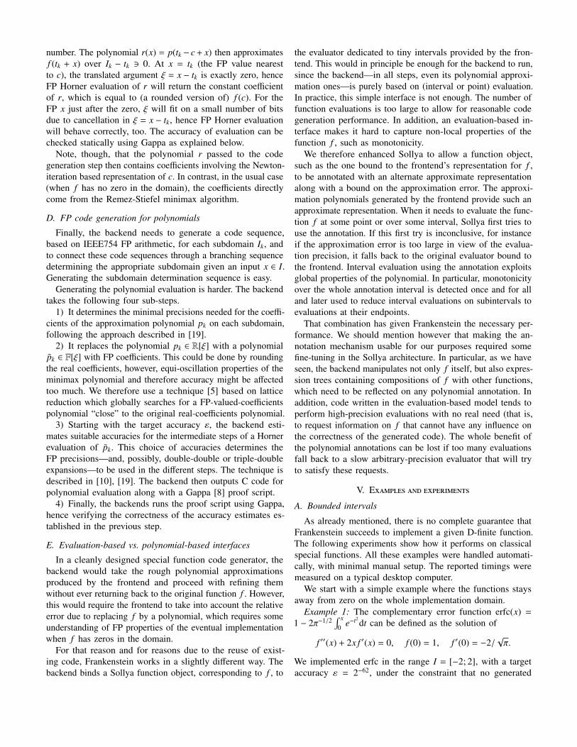
The Voigt profile V(x) (Figure 3) is a probability distributionused in particular in spectrography, and whose computationhas been the subject of abundant literature [27], [30]. It de-pends on two parameters λ, σ > 0 and is defined for x ∈ R asa convolution of a Gaussian distribution and a Cauchy distri-bution,

V(x) =1

σ√

2π

λ

π

∫ +∞

−∞

exp −x2

2σ2

(x − t)2 + λ2 dt.

A change of variable yields the alternative expression

V(x) =1

σ√

2π

λ

π

∫ +∞

−∞

exp (u−x)2

2σ2

u2 + λ2 du, (11)

and it is not hard to see that (11) satisfies⎧⎪⎪⎪⎪⎪⎪⎨⎪⎪⎪⎪⎪⎪⎩σ4V ′′(x) + 2σ2V ′(x) + (x2 + λ2 + σ2)V(x) =

λ

π,

V(0) =1

σ√

2πexp

(λ2

2σ2

)erfc

(λ

σ√

2

), V ′(0) = 0.

(12)

(To remain in our general setting, a homogeneous ODE canbe derived by differentiating one more time.)

The Voigt profile with arbitrary parameters can be expressedin terms of the Faddeeva function, itself a renormalizationof the complex error function. A general implementation ofthese functions, due to Johnson [17], is used for instance inthe standard library of the Julia programming language. Herewe are interested in implementing the function V(x) for fixedλ and σ, with an overall relative accuracy ε = 2−45. In ourexperiment, we take σ = 1 and λ = 1

2 , but the method appliesverbatim to any moderate rational values.

We start with generating an implementation for x ∈ [0; 10].With approximations having at most 11 nonzero coefficients,[0; 10] is split into 33 subdomains of width varying from about0.1 around x = 5 to about 0.6 near the endpoints.

For large x, however, the computation of polynomial approx-imations starting with the initial values at 0 as described inSection III is no longer feasible. Also, it would not make anysense to split [10; 21024] into small subintervals. An obviousremedy is to consider f (ξ) = V(1/ξ) on (0, 0.1). A change ofvariable in (12) shows that

σ4ξ6 f ′′(ξ)+2σ2ξ3(σ2ξ2−1) f ′(ξ)+(λ2ξ2+σ2ξ2+1) f (ξ) =λξ2

π.

This equation has an irregular singular point at 0, beyond thescope of the polynomial approximation method we discussed.Nevertheless, looking for solutions as formal power seriesyields a unique divergent series (compare to [13])

ξ2L(ξ) = ξ2 + (2σ2−λ2) ξ4 + (1σ4−10σ2λ2 +λ4) ξ6 + · · · (13)

whose coefficients again satisfy a simple linear recurrence. It iswell-known that such formal solutions at infinity are asymptoticexpansions of “true” analytic solutions and provide good ap-proximations for large x [26]. In the present case, the solutionsof the homogeneous part of the equation decrease exponen-tially as ξ → 0, ξ > 0, so all solutions of the homogeneousequation share the same asymptotic expansion (13).

With our values of σ and λ, we estimated that the polyno-mial L obtained by truncating L(ξ) to the order 90 satisfies|L(1/x) − x2V(x)| < 2−65 for all x > 10. For the purposes ofthis experiment, this truncation order was found numerically.Rigorous bounds could likely be derived by the method ofOlver [26, Chap. 7]. NumGfun does not support evaluationsnear irregular singular points, but as L(ξ) stays away from zeroon [0, 0.1], we could directly pass it to the Frankenstein back-end. The resulting code uses two polynomials of degree 11with floating-point coefficients.

We then manually combined the two automatically generatedcodes into implementation that works correctly on the wholeof F. The Voigt function is even, so the final code startsby dropping the sign of the argument. Based on a simplecomparison, it then calls either the code for V(x) around zeroor computes ξ = 1/x (in double precision) and calls the codefor V(1/x) around zero.

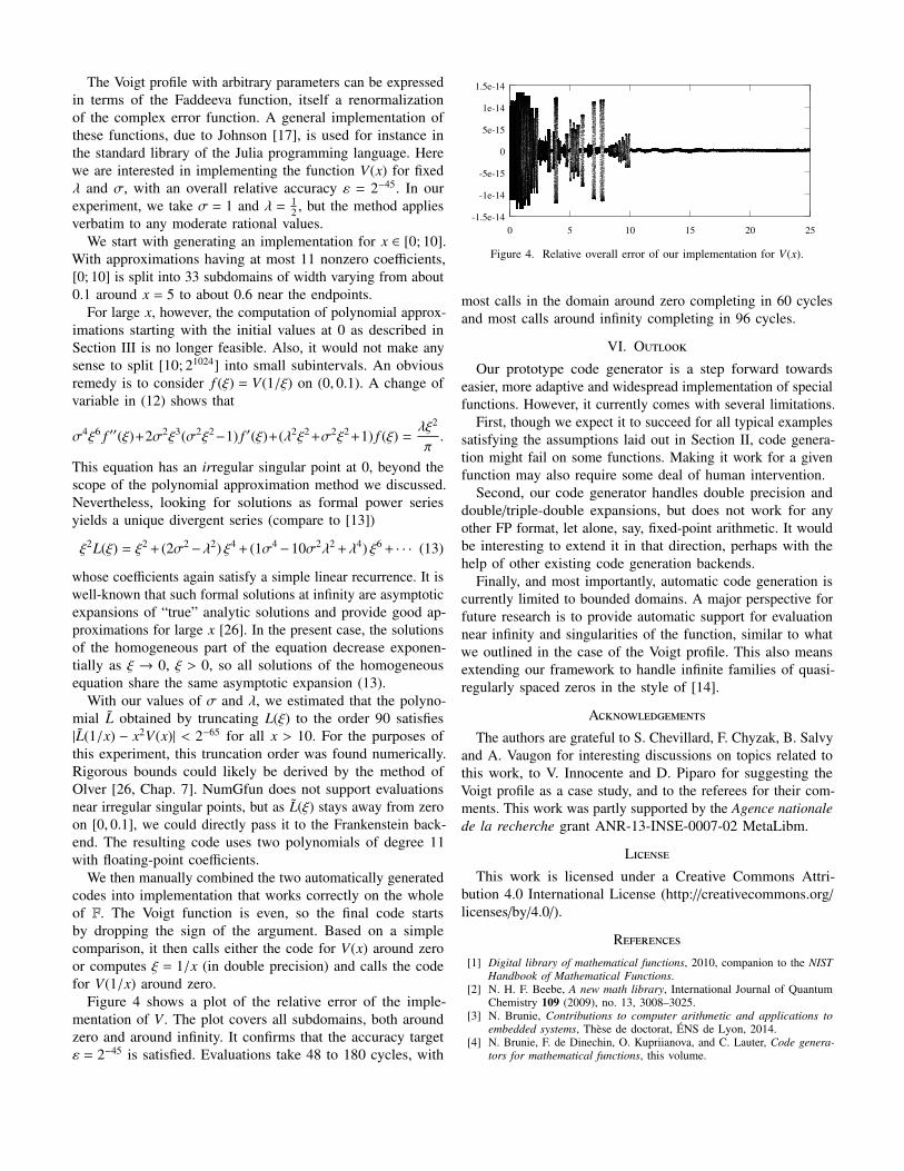
Figure 4 shows a plot of the relative error of the imple-mentation of V . The plot covers all subdomains, both aroundzero and around infinity. It confirms that the accuracy targetε = 2−45 is satisfied. Evaluations take 48 to 180 cycles, with

-1.5e-14

-1e-14

-5e-15

0

5e-15

1e-14

1.5e-14

0 5 10 15 20 25

Figure 4. Relative overall error of our implementation for V(x).

most calls in the domain around zero completing in 60 cyclesand most calls around infinity completing in 96 cycles.

VI. Outlook

Our prototype code generator is a step forward towardseasier, more adaptive and widespread implementation of specialfunctions. However, it currently comes with several limitations.

First, though we expect it to succeed for all typical examplessatisfying the assumptions laid out in Section II, code genera-tion might fail on some functions. Making it work for a givenfunction may also require some deal of human intervention.

Second, our code generator handles double precision anddouble/triple-double expansions, but does not work for anyother FP format, let alone, say, fixed-point arithmetic. It wouldbe interesting to extend it in that direction, perhaps with thehelp of other existing code generation backends.

Finally, and most importantly, automatic code generation iscurrently limited to bounded domains. A major perspective forfuture research is to provide automatic support for evaluationnear infinity and singularities of the function, similar to whatwe outlined in the case of the Voigt profile. This also meansextending our framework to handle infinite families of quasi-regularly spaced zeros in the style of [14].

Acknowledgements

The authors are grateful to S. Chevillard, F. Chyzak, B. Salvyand A. Vaugon for interesting discussions on topics related tothis work, to V. Innocente and D. Piparo for suggesting theVoigt profile as a case study, and to the referees for their com-ments. This work was partly supported by the Agence nationalede la recherche grant ANR-13-INSE-0007-02 MetaLibm.

License

This work is licensed under a Creative Commons Attri-bution 4.0 International License (http://creativecommons.org/

licenses/by/4.0/).

References[1] Digital library of mathematical functions, 2010, companion to the NIST

Handbook of Mathematical Functions.[2] N. H. F. Beebe, A new math library, International Journal of Quantum

Chemistry 109 (2009), no. 13, 3008–3025.[3] N. Brunie, Contributions to computer arithmetic and applications to

embedded systems, Thèse de doctorat, ÉNS de Lyon, 2014.[4] N. Brunie, F. de Dinechin, O. Kupriianova, and C. Lauter, Code genera-

tors for mathematical functions, this volume.

[5] S. Chevillard, Évaluation efficace de fonctions numériques. Outils etexemples, Thèse de doctorat, ÉNS de Lyon, 2009.

[6] S. Chevillard, M. Joldes, , and C. Lauter, Sollya: An environment for thedevelopment of numerical codes, ICMS 2010 (K. Fukuda et al., eds.),LNCS, vol. 6327, Springer, 2010, p. 28–31.

[7] D. V. Chudnovsky and G. V. Chudnovsky, Computer algebra in the ser-vice of mathematical physics and number theory, Computers in Mathemat-ics (D. V. Chudnovsky and R. D. Jenks, eds.), Dekker, 1990, p. 109–232.

[8] F. De Dinechin, C. Lauter, and G. Melquiond, Certifying the floating-point implementation of an elementary function using Gappa, IEEETransactions on Computers 60 (2011), no. 2, 242–253.

[9] F. de Dinechin, M. Joldes, and B. Pasca, Automatic generation ofpolynomial-based hardware architectures for function evaluation, ASAP2010, p. 216–222.

[10] F. de Dinechin and C. Lauter, Optimizing polynomials for floating-pointimplementation, Real Numbers and Computers (RNC 8), 2008, p. 7–16.

[11] L. Fox and I. B. Parker, Chebyshev polynomials in numerical analysis,Oxford University Press, 1968.

[12] A. Gil, J. Segura, and N. M. Temme, Numerical methods for specialfunctions, SIAM, 2007.

[13] J. A. Gubner, A new series for approximating Voigt functions, Journalof Physics A: Mathematical and General 27 (1994), no. 19, L745.

[14] J. Harrison, Fast and accurate Bessel function computation, ARITH 19(J. D. Bruguera et al., eds.), IEEE, 2009, p. 104–113.

[15] E. Hille, Ordinary differential equations in the complex domain, Wiley,1976, Dover reprint, 1997.

[16] IEEE Microprocessor Standards Committee, Floating-Point WorkingGroup, IEEE standard for floating-point arithmetic, 2008, Second edition.

[17] S. G. Johnson, Faddeeva package, 2012.[18] O. Kupriianova and C. Lauter, Metalibm: A mathematical functions code

generator, ICMS 2014 (H. Hong and C. Yap, eds.), LNCS, vol. 8592,Springer, 2014, p. 713–717.

[19] C. Lauter, Arrondi correct de fonctions mathématiques – fonctions uni-variées et bivariées, certification et automatisation, Thèse de doctorat,Université de Lyon – ÉNS de Lyon, 2008.

[20] J. H. Mathews, Bibliography for Taylor series method for D.E.’s, 2003.[21] M. Mezzarobba, NumGfun: a package for numerical and analytic com-

putation with D-finite functions, ISSAC ’10 (S. M. Watt, ed.), ACM,2010, p. 139–146.

[22] M. Mezzarobba and B. Salvy, Effective bounds for P-recursive sequences,Journal of Symbolic Computation 45 (2010), no. 10, 1075–1096.

[23] S. L. Moshier, Cephes mathematical function library, 1984–.[24] J.-M. Muller et al., Handbook of floating-point arithmetic, Birkhäuser,

2010.[25] M. Neher, K. R. Jackson, and N. S. Nedialkov, On Taylor model based

integration of ODEs, SIAM Journal on Numerical Analysis 45 (2007),no. 1, 236–262.

[26] F. W. J. Olver, Asymptotics and special functions, A K Peters, 1997.[27] F. Schreier, The Voigt and complex error function: a comparison of com-

putational methods, Journal of Quantitative Spectroscopy and RadiativeTransfer 48 (1992), no. 5, 743–762.

[28] J. R. Shewchuk, Adaptive precision floating-point arithmetic and fastrobust geometric predicates, Discrete & Computational Geometry 18(1997), no. 3, 305–363.

[29] P. H. Sterbenz, Floating-point computation, Prentice-Hall, 1974.[30] W. J. Thompson et al., Numerous neat algorithms for the Voigt profile

function, Computers in Physics 7 (1993), no. 6, 627–631.[31] J. van der Hoeven, Fast evaluation of holonomic functions, Theoretical

Computer Science 210 (1999), no. 1, 199–216.[32] , Fast evaluation of holonomic functions near and in regular sin-

gularities, Journal of Symbolic Computation 31 (2001), no. 6, 717–743.