SEMI-ANNUAL PROGRESS REPORT

ON

DISTRIBUTED ACTIVE CONTROL

OF

LARGE FLEXIBLE SPACE STRUCTURES (Grant # NAG 5-749)

Submitted by

/ Dr. Charles C. Nguyen, Principal Investigator

Dr. Amr Baz, Principal Investigator The Catholic University of America

Washington, D. C. 20064

to

Dr. Joseph V. Fedor Code 712 Space Technology Division Goddard Space Flight Center Greenbelt, Maryland 20771

November 1986

https://ntrs.nasa.gov/search.jsp?R=19870004043 2018-06-16T23:45:28+00:00Z

TABLE OF COMENTS

PAGE

Sumar y

Symbols and Notations

1. Introduction

2. Updated Research

3.

4. Project Research Results

5. Current and Future Research

6. Conclusion

Modeling o f The Polar Platform

References

Figures and Tables

4

5

16

16

20

21

- 1 -

S M R Y

T h i s p rogres s r e p o r t summarizes t h e research work performed a t t h e

Ca tho l i c Universi t y of h e r i c a on t h e research g ran t e n t i t l e d 'Distributed

Active Control of Large F l e x i b l e Space S t ruc tu res , ' funded by W W G o d d a r d

Space F l i g h t Center, under the gran t number NAG 5-749, dur ing t h e pe r iod of

March 19, 1986 t o September 19, 1986.

I n t h i s r e p o r t w e f i r s t update t he r e sea rch work relevant to t h e

p r o j e c t .

s t a t e d . The r e p o r t is then concluded by a d i scuss ion o f current and future

research work

Then t h e research accomplished du r ing t h e above per iod w i l l be

- 2 -

SYMBOLS MJD NMATl ON

MI 0 ... 0 M 2 . . . . . . . . . 0 0

= an (mxn) zero matrix 3* Omxn

4. In = an (nxn) ident i ty matrix

5. x ( t ) = 9 x ( t ) dt

0

0

MN

- 3 -

1. Introduction

The advent of a space transportation system, such as the space shuttle

makes i t possible to conceive of very large satellites and spacecraft which

could be carried into space and deployed, assembled, or constructed there

for such diverse purposes as comnunications, surveillance, astronomy, space

exploration, and electric power generation 121. These large space

structures (LSS) concepts range from central rigid bodies, to the solar

electric propulsion spacecraft and the generic polar platform. Two control

problems for LSS are attitude control and shape control (241. The former

involves maintaining a given orientation of the spacecraft, e.g., with

respect to the sun or earth; the latter involves maintaining the shape of

critical structures of LSS. LSS are distributed parameter systems that

possess many low resonant frequencies and have very stringent requirements

f o r shape, orientation, alignment, vibration suppression and pointing

accuracy. These requirements lead the control designers to the concept of

active control of LSS with various sensors and actuators located about the

structure and operating through on-line computer controllers to tailor the

performance and behavior of the system.

There has been considerable interest in the area of active control o f

LSS [11-[243. A number o f control schemes were proposed for large flexible

space structure (LFSS), but they all represent on0 form or another of modal

control 1113. Two main modal control schemes are the coupled Modal Control

and Independent Modal Space Control (IMSC).

controller consisting o f a state estimator and a state feedback law; the

latter controls each mode independently by means of the modal filter [13].

The former employs an active

- 4 -

I n th is repor t we f i r s t update the research i n ac t i ve con t ro l o f LFSS

t o provide a mathematical framework f o r the pro ject .

a generic polar p la t form i s developed using f i n i t e element method.

that some pro jec t research r e s u l t s are presented. We then discuss the

current and fu tu re research e f fo r t .

2. UDdated Research

Then the modell ing o f

A f te r

A conclusion w i l l sumar ize the repor t .

I n th is sect ion we f i r s t present the mathematical descr ip t ion o f l a rge

space s t ructures (LSS) and then discuss the two main cont ro l schemes f o r

th is type o f structures.

2.1 Mathematical DescriDtion o f LSS

The LSS may be described as a continuum by the fo l low ing p a r t i a l

d i f f e r e n t i a l equations

2

M ( p p u ( P f t ) + L u ( P , t ) = f ( P , t ) 2 a t (2.1)

where u(P,t) = displacement o f an arb i t ra ry po int e L = Linear d i f f e r e n t i a l se l f -ad jo in t operator o f

order 2p, expressing the system s t i f fness .

M(P) = d i s t r i bu ted mass

f (P , t ) = d i s t r i bu ted cont ro l force

Equation (2.1) must be s a t i s f i e d at every po int P i n the domain D. The

displacement o f u(P,t) ir subject t o the boundary condi t ions

ai u ( ~ , t ) = 0 for i=1f2f...fp

where Bi are l i nea r d i f f e r e n t i a l operator o f order ranging f r o m

0 t o (Pp-1).

(2.2)

- 5 -

The essocieted eigenualue problem

L @,(PI = x, M(P) (Pr(P)

€or r=112,.. . ,w

with the boundary conditions

Bi = 0

for i=112f...1p; r=l12,...,d

is formulated by

(2.3)

( 2 . 4 )

where x is the rth eigenvalues and (0 (p ) is the eigenfunction associated

with 1 . Sometimes @ (p)is called the mode shape. r r

r r

Equations (2.3) and (2.4) can be solved to obtain the solutions of and r

and in addition, if the operator L is positive definite, then all @ r

eigenvalues are positive. The mode frequency (or natural frequency) is

defined as 4

using expansion theorem [ l i l , the solution of u(P,t) can be obtained as

r=l where ur(t) satisfies

- 6 -

for r=1,2,. . .

I n pract ice, the i n f i n i t e ser ies i n (2.6) i s truncated as

u(P,t) = : r=l

(2.9)

where M i s chosen t o be s u f f i c i e n t l y large so that u(P,t) can be represented

w i t h good f i d e l i t y .

Since M may be qu i te large, i t is not reasonable t o con t ro l a l l M

modes. Hence we select N modes t o control . These N modes are c a l l e d

Control led Modes. The remaining R modes (R = M-N) are ca l l ed Residual Modep

(uncontrol led modes).

Equation (2.7) can be transformed in to the s ta te equation form as

fo l lows

T . . where xc(t) = fu, u2 ... u1 u2 ... UNI (2.12)

WIECEDWQ PAGE BLANK MOT FILMED - 7 -

Discrete Actuators: Since i t is impossible to implement distributed

control forces, the distributed control force f(P,t) is realized by k

discrete point force actuators

where S(P-Pi) is a spatial Dirac Delta function.

Substi tuting (2.18) into (2.8) y i e l d s

k

i=l f (t) - = 1 @,(pi) ~ ~ ( t ) ; r=1,2,. r

Now using (2.19) we obtain

B = C

(2.18)

(2.19)

(2.20)

(2.21)

(2.22)

(2.23)

- 8 -

T and F ( t ) = IF1 F2 .... FkI (2.24)

Discrete Sensors: Suppose there are s discrete sensors consis t ing o f p

ve loc i ty sensors, located a t p locat ions Pvl Pup, ..., pup and 9

displacement sensors, located a t q locat ions PD1, PD2, ..., PDqe

(2.9) we can express the veloci ty sensor output as

Using

(2.25)

f o r j = 1,2,.. ., p, and the displacement sensor output as M

F l = u(P ,t) = 1 @=(PDj) u p ) (2.26)

Dj

for j = 1,2,..., q.

i f we def ine the sensor output vector as

T y(t) = [Y, Y2 - - . Yp YPl Ype2 - . - Ywsl I

then using (2.25) and (2.261, we can wr i te

where

(2.27)

(2.29)

(2.30)

(2.31)

(2.32)

(2.33)

- 9 -

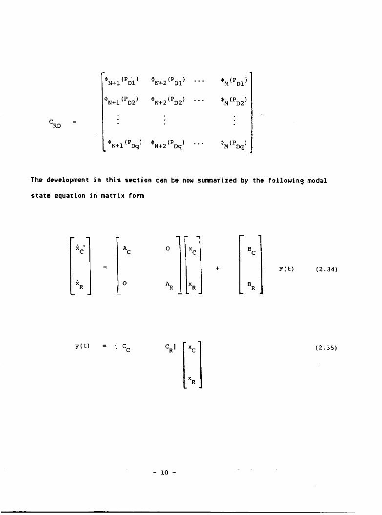
The development in this section can be now summarized by the following modal

state equation in matrix form

C A [j = 1 - 0 Y ( t ) = [ cc

0

A R ][:I + (2.34)

(2.35)

- 10 -

2.2 The CouDled Modal Control Scheme

In this scheme, the active controller consists of two parts:

a) a state estimator that accepts the sensor output y(t) and produces

an estimate Xc(t) of the controlled state XC(t) and

b) a linear state feedback control law that multiplies the estimated

controlled state XC(t) by constant gain to produce the actuator input F(t).

The state estimator can be of the Luenberger type that is described by

E 151

(2.36)

The state estimator error is defined as

eC(t) = xC(t) - xC(t) A (2.37)

Theref ore 0

0 A h eC(tl = x(t) - xc(t) = (AC - 0 c c C )e c (t) t GCCRxR(t) (2.38) The linear state feedback la is defined by

A F(t) = KC xC(t) (2.39)

Now substituting (2.39) into (2.34) and (2.381, we obtain the composite

state equation as follows:

0 AC+BCKC BCKC

GCCR A -G C c c c 0

A 'RKC BRKC R

The objective o f the couple modal control scheme ir to select KC and Gc ouch

that the composite system (2.40) is asymptomatically stable. In (2.40) the

- 11 -

control spillover is represented by BR and the observation spillover is

represented by CR.

Figure 1.

2.3 The IndeDendent Modal %ace Control Scheme (IMSC)

The coupled modal control scheme is illustrated in

The IMSC scheme was developed by Meirovitch and others [ l o ] to control

each mode independently. First an auxiliary variable U (t) is defined by r v p = 1/0 q t ) (2.41)

Therefore using (2.7) we can write 2 r

Now using (2.41) and (2.421, we obtain

i r p = l / U r iir(t) = - w u p + f r ( t ) (2.42)

(2.43)

(2.44)

= [ O 'r

T and xr = [ur vr1

T f r 'Wrl (2.45)

(2.46)

The essence o f the IMSC is to choose Ur such that Wr depends only on 0;

alone: wr = W r ( w r ) (2.47)

The optimal design of Wr was discussed in 1121.

Modal Filter; To implement the IMSC scheme, the modal displacements

ur(t) and modal velocities ur(t) are required.

filter accepts the measurements o f displacement u(P,t) and ueiocity u(P,t)

at every point P at all time and produces the modal displacement ur(t) and

- 12-

A device, called modal

modal velocity ur(t).

given by

The mathematical representation o f a modal filter is

( 2 . 4 8 )

( 2 . 4 9 )

I t is noted that distributed sensors are needed to obtain the

displacements u(P,t) and velocities u(P,t).

Implementation of IMSC usins discrete activators and sensors

The implementation of IMSC requires distributed control, i.e. Control

forces are applied at every point of the structure, and also requires

distributed sensors, i.e. the displacements and velocities are measured at

every point.

actuators and discrete sensors are used instead.

This is however not realizable in practice. Thus discrete

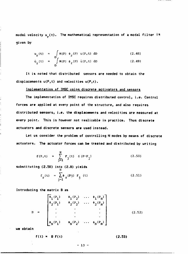
Let us consider the problem o f controlling N modes by means of discrete

actuators. The actuator forces can be treated and distributed by writing

substituting (2.50) into (2.8) yields N

Introducing the matrix B as

B =

we obtain

... 8

f(t) = B F(t)

- 1 3 -

( 2 . 5 0 )

( 2 . 5 1 )

( 2 . 5 2 )

(2.53)

where T f(t) = If, f2 .... f,l I F(t) = [F, F2 .... FNl

(2.54)

(2.55)

Suppose B is nonsingular, then the actual control vector F(t) can be

synthesized from the generalized control vector f(t) by

F(t) = B* f(t) (2.56)

Next let us assume there are m sensors capable of measuring

displacements and velocities at the discrete points P=Pk (k=1,2,...,m).

Then from these measurements the entire displacement pattern u(P,t) and

velocity pattern u(P,t) can be estimated by using various interpolation

functions. The structure of the IMSC scheme using discrete actuators and

sensors is shown in Figure 2.

2.4 Evaluation of the control schemes

The design of the coupled modal control scheme is straight forward

since i t is simply a pole placement problem if the observation spillover is

negligible.

composite system are the eigenvalues o f ( A c t BCKi; (AC-GCCC)and AR due to

block triangularity. There are several techniques such as in [15,16 1 that

Indeed if we set CR=O in (2.4), then the eigenvalues of the

help the control designer to select KC and Gc such that 6tcC+BcKc and Ac-QcCc

have desired eigenvalues. The control spillover is represented by . (2.57)

Since eC(t) and x (t) will decay to zero, the control spillover will cause

unwanted excitations of the residual modes, but i t cannot shift the residual C

mode frequencies. Consequently the control spillover results in some

- 1 4 -

unwanted oscillations of the residual modes. So when the observation

spillover is absent, then the control spillover degrades the system

responses but cannot destabilize the system.

When observation spillover exists, then instability may occur when some

of the eigenvalues of the composite system (2.40) are unstable.

The control and obsesrvation spillover can be minimized if the

actuators and sensors are located at (or very near to) the zero o f the mode

shapes of the residual modes. This concept is limited since it creates

uncontrollable and unobservable triple (AC, Bc, Cc) that hinders the design

o f state estimators and state feedback laws. In addition, the freedom to

locate sensors and actuators arbitrarily is rarely available to the designer

since these locations are often already determined by structural

considerations. I

I t is well known 1121 that the IMSC scheme is capable of eliminating

control and observation spillover. However i t requires the implementation

of distributed actuators and distributed sensors that unfortunately cannot

be provided by the current state-of-the-art. Consequently, discrete

actuators and discrete sensors have to be used. A question that is still

not clearly answered is how many discrete actuators and sensors are

necessary for a successful implementation of the IMSC scheme. In addition,

the IMSC scheme when being implemented by discrete actuators also has

control spillover into the uncontrolled modes. However as pointed out in

[12], the control spillover effect is not very important.

Both control schemes, the coupled modal control and the IMSC require

- that a closed-form solution of the eigenvalue problem exist. Unfortunately

the vast majority o f continuous system% icads to eigenvaiue problems that do

not have closed-form solutions, owing to nonuniform mass or stiffness

- 15 -

d is t r i bu t i ons , Hence i n t h i s case, i t i s necessary t o seek approximate

solut ions of the eigenvalue problem.

3. Modelinq o f the Polar Platform

One of the p ro jec t a c t i v i t i e s i s t o obtain a model f o r a generic polar

plat form whose phys ica l parameters are given i n Table 1.

A MSTRAN f i n i t e element analysis package (McNeal Schwendler version)

was employed to model the plat form and i t s appendages by 52 modes.

model i s i l l u s t r a t e d i n Figure 3.

The

The plat form i t s e l f was modeled by 28

nodes, the so lar panel and the astromast by 16 nodes and the engineering

module by 8 nodes.

I n the developed model, the payload ca r r i ed by each module was assumed

t o be d i s t r i b u t e d uni formly throughout a l l nodes. Also the engineering

module was assumed t o be very r i g i d as compared t o the p la t form or the solar

panel . The model considers only those degrees o f freedom o f the p la t form that

cont r ibute t o i t s bending and tors ional v ibrat ions.

Table 2 l i s t s the f i r s t ten modes o f Vibrations. The f i r s t two na tura l

frequencies are the f i r s t r i g i d body modes i n p i t c h i n g and r o l l i n g . The

remaining modes are the f l e x i b l e modes o f the plat form.

I t can be seen that the f l e x i b l e modes are very low and h igh ly

condensed over a narrow band between 0.054Hz and 0.448 Hz. A sample o f the

f i r s t three modes o f v ibrat ions are shown i n Fig. 4-6.

4. Project Research Resul t t

I n th is sect ion we w i l l present some research r e s u l t s obtained by the

p r inc ipa l investigators during the research period s ta ted in the summary.

One o f the p ro jec t object ives i o t o evaluate several candidate cont ro l

- 16 -

schemes in order to select the most appropriate control scheme for the LFSS.

The study of coupled-modal control and Independent Modal Space Control

involves in such problems as pole allocation, eigenvalue assignment, state

estimator design, canonical transformation etc. ... . During the

investigation of the above topics, some results have been found and are

sumar i zed bel ow.

4.1 Canonical Transformation

Canonical transformation has been proven to be very useful in the

design of state estimators and state feedback. In 1141 two canonical

transformations were deweloped for a class of time-varying multivariable

control systems. Since most physical systems such as LFSS are time-varying

in nature, this type o f time-varying canonical transformations will be very

helpful in design of more practical control schemes for LFSS.

4.2 Eisenvalue Assiqnment and Pole Allocation

The eigenvalue assignment or pole allocation problem is very essential

to the control of LFSS since i t is related to the system stability. Two

comon problems in control system design for LFSS are the selection of a

state feedback gain to shift the natural modes of the LFSS to a set o f

desired damping modes, and the design of a state estimator whose eigenvalues

can be arbitrarily assigned. These two problems can be treated as

eigenvalue assignment or pole allocation problems. In E161 it was shown

that eigenvalues can be arbitrarily assigned to a class o f time-varying

multivariable systems. Canonical transformation developed in [141 was

employed to design the state feedback gain. The distributed control problem

was considered in [17] where a control scheme was developed to arbitrarily

afiocate closed-loop poles to a distributed time-inuariant system that is

con trolled by several pairs o f sensors and actuators.

- 17 -

4.3 State Estimator Desisn

State estimator design is very crucial to the control of LFSS since the

controlled state vector has to be estimated for the coupled modal control

case and the modal state for the IMSC case. In 1181 a neu algorith was

proposed to design reduced-order state estimators for a class of

time-varying multivariable control systems that are uniformly observable.

The result in [18] is an extension o f that in 1151 where a full-order state

estimator was designed.

4.4 Simulation of Control Schemes

Since the generic polar platform is relatively a complicated structure,

we start the study of the control scheme by considering the control of a

simply supported bean with one actuator and one sensor. Complete

understanding of the control of this simply supported bean will help us to I

I gain some insight o f the control of the complete structure. The bean

dynamics are modelled by the Euler-Bernoulli partial differential equation

2 u ( x , t ) + E1 ---- a4 u ( x , t ) = f ( x , t ) a

a t ax 4 m ---- ( 4 . 1 )

For simplicity we set the mass m, the moment of inertia I, the modulus of

elasticity E and the length of the bean to unity. The boundary conditions

for this simply supported bean are

2

2 a -

ax

2

2 a - - -u(O,t) = - - - u ( l , t ) = 0

ax

- i a -

and

The eigenvalue solutions for this case are 2

w = (kn) k

Ok = s i n ( k i x )

The beam is controlled by a single point actuator at x = 1/6:

.s f ( x , t ) = (1/2) 6 ( x - 1/61 f ( t ) ( 4 . 6 )

and the displacement is measured by a single point sensor located at x =

W 6 :

y(t) = u(W6,t) (4.7)

Using the Matlab and the control tool box software package, an active I

controller was designed to control the first three modes o f the bean. To

minimize the following unweighted energy

J J E ( t 1 t 0.1f2(t)ldt (4.8)

the control gain was determined to be

KC = [-3.87 -3.86 -3.86 -1.01 -6.08 -20.31 (4.10)

A state estimator was designed to estimate the controlled modes. The

state estimator gain G given below: C

Gc = 1711.8 52.34 -7.39 10.06 -5.97 1.981 (4.11)

- 19 -

w i l l assign s tab le eigenvalues t o the s tate estimator. Several s imulat ion

runs were made t o study the performance o f the ac t ive cont ro l le rs and the

e f f e c t o f the contro l and observation sp i l lover .

I n a l l simulat ion runs, an impulse disturbance was created t o exc i te

the system.

sp i l l ove r .

reach the zero steady state.

caused by cont ro l sp i l lover i n t o the uncontrol led modes.

observation ex i s t s i n t h i s case, the system i s t i l l stable. Fig. 10 and 11

display the sensor output and actuator input when no sp i l lover ex is ts . We

no t i ce that the displacement war decayed t o zero.

i n t o the 4 t h and 5 th uncontrol led modes i s i l l u s t r a t e d i n Fig. 12 and 13,

respect ive ly . The eigenvalues o f the composite system [Equation (2.4011 f o r

a l l poss ib le cases o f sp i l lover are given i n Table 2a.

eigenvalues o f the closed-loop system, the s ta te estimator, con t ro l led

subsystem and uncontrol led subsystem.

Figures 8 and 9 present the e f f e c t s o f control and observation

We note that when sp i l l ove r exists, the displacement did not

I t has an o s c i l l a t i o n w i t h small amplitude

Even though the

The contro l sp i l l ove r

Table 2b shows the

I n Table 3a we note that when no observation sp i l lover ex is ts , the

eigenvalues o f the composite system consist o f the eigenvalues o f the

closed-loop system, the s tate estimator, and the uncontrol led subsystem.

Th is agrees w i t h the discussion made i n Section 2.3.

5. Current and Future Research

Continuing the research stated i n Section 4, we current ly focus on the

study o f sp i l l ove r minimization.

r e s u l t s showed that the system performance i s degraded at the presence o f

con t ro l sp i l l ove r . The LFSS can also become unstable i f the observation

As we have seen, the system simulat ion

spillover exists. Therefore spillover minimization study is very crucial to

the control of LFSS. We are investigating the minimization of the spillover

by

(a) Proper locating of actuator and sensors.

(b) Determining a sufficient number o f actuators and sensors needed.

(c) Applying the IMSC method to the generic polar platform.

The above study is carried out mostly by simulating the system for

various situations using system simulation languages in order to set up a

guideline for selecting and locating actuators and sensors.

After the control of the simply-supported bean has been studied

throughout, we will apply the resulting control scheme to the complete

generic polar platform.

be addressed in the future research:

Several control issues such as given below should

(a) Evaluation of the application of coupled-modal control and IMSP to

the generic polar platform in terms of feasibility, reliability, spillover,

and computational effort.

(b) Implementation of an adaptive control scheme for the system.

(c) Study of a robust controller when the system parameters are not

well-known and when unpredictable disturbances are expected.

6. Conclusion

In this report we first updated the research related to project.

modelling o f the generic polar platform using finite element method was

discussed.

study using computer simulation and some theoretical research results o f

such problems as eigenvalues, state estimator, and state feedback design.

Current research effort was discussed and future research activities were

The

We then presented some preliminary results o f the control system

assessed.

- 21 -

References

1.

2.

3.

4.

5.

6.

7.

8.

9 .

10.

11.

12.

13.

M.J. Balas, 'Active Control o f F lex ib le Systems,' J. Optimization Theory and Applications, U o l . 25, No. 3, pp 415-436, July 1978.

M.J. Balas, 'Trends i n Large Space Structure Control Theory: Fondest Hopes, Wildest Drems,' IEEE Trans. Automat. Control., AC - 27, No. 3. pp. 522-534, June 1982.

Michel A. Floyd, 'Coment on a Comparison o f Control Techniques f o r Large F l e x i b l e Systems,' J. pp. 634-635, 1984.

o f Guidance and Control, Uol. 7, No. 5,

A. L. Hale and G. A. Rahn, 'Robust Control o f Sel f - Adjoint D is t r i bu ted - Parameter Structures,' J. 7, No. 3, pp. 263-273, 1984.

o f Guidance and Control, Uol.

P. C. Hughes and R. E. Skelton, 'Con t ro l l ab i l i t y and Observabil ity f o r F lex ib le Spacecraft,' J. o f Guidance and Control, Uol. 3, pp. 452-459, Oct. 1980.

D. J. Inman, 'Modal Decoupling Conditions f o r D is t r ibu ted Control o f F lex ib le Structures,' J. o f Guidance and Control, Uol. 7, No. 6, pp. 750-752, 1984.

T. L. Johnson, 'Progress i n Modelling and Control o f F lex ib le Spacecraft,' Journal o f the Frankl in I n s t i t u t e , U o l . 315, No. 516, pp. 495-520, May/June 1983.

S. Kumar and J . H. Seinfeld, 'Opt ima l Locat ion o f Measurements f o r D is t r ibu ted Parameter Estimation,' IEEE Trans. Automat. Control, AC - 23, No. 4 , pp. 690-698, Aug. 1978.

L. Meirovi tch, and H. Baruh, 'On the problem o f observation s p i l l o v e r i n D is t r i bu ted - Parmeter Systems,' Journal o f Optimization Theory and Applications, Uol 39, No. 2, pp. 611-620.

L. Mei rou i tch and H. Baruh, 'Control o f Se l f -Ad jo in t D is t r ibu ted - Parameter Systems,' J. o f Guidance and Control, Vo l . 5, No. 1, pp. 60-66, Feb. 1982.

L. Me i rov i tch and H. Or , 'Modal Space Control o f D is t r ibu ted Gyroscopic Systems,' J . o f Guidance and Control, Uol. 3, No. 2, pp. 140-150, A p r i l 1380 . L. W i r o v i t c h and others, ' A Comparison o f Control Techniques for Large F l e x i b l e Systems,' J. o f Ouidancs, Control, and Dynaaics, Voi . 6, pp. 302-30, July - Clug. 1983.

L. Me i rov i tch and H. Baruh, 'Tho Implementation o f nodal F i l t e r s f o r

- 2 2 -

Control of Structures,' J . o f Guidance and Control, V o l . 8, No. 6, pp, 707-716, Dec. 1985.

14. C. C. Nguyen, 'Canonical Transformation for a c lass o f Time - Varying Mu l t i va r iab le Systems,' I n t . J . Control, V o l . 43, No. 4, pp. 1061-1074, A p r i l 1986.

15. C. C. Nguyen, 'Design of State Estimator for a Class o f TimeYarying Mul t i var iab le Systems,' IEEE Trans. Automat. Control, AC-30, Feb. 1985.

16. C. C. Nguyen, 'Arb i t rary Eigenvalue Assignments for Linear Time-Varying Mul t i var iab le Control Systems,' t o appear i n I n t . Journal o f Control, 1987.

17. C. C. Nguyen, 'Pole A l loca t ion for Decentralized-Control Systems,' Proc. I n t . Conf. Modell ing and Simulation, MSF, Williansburg, Sept. 1986.

18. C. C. Nguyen, 'Design o f Reduced - Order State Estimators for Linear Time - Varying Mul t i var iab le Systems,' submitted for pub l ica t ion i n I n t . Journal o f Control, 1986.

19. D. Schaechter, 'D is t r ibuted Control o f Large Space Structures,' Jet I Propulsion Lab Report, #81-15, May 1981.

20. D. Turner and H. M. Chun, 'Optimal D is t r ibu ted Control o f a f l e x i b l e Spacecraft During a Large - Angle Maneuver,' J . of Guidance, and Dynamics, Vo l . 7, No. 3, pp. 257-264, 1984.

Control,

21. Sa h a t u , 'Optimization o f Sensor and Actuator Locations i n a D is t r ibu ted Parameter System,' Journal o f the Frank l in I n s t i t u t e , V o l . 315, No. 516, pp. 407-421, May/Juna 1983.

22. H. 02, and others, 'Some Problems Associated w i t h D i g i t a l Control o f Dynamical Systems,' J . o f Guidance and Control, Uol. 3, No. 6, pp. 523-528, Dec. 1980.

23. H. E. Vandet Velds, and C a R. Cariguau, 'Number and Placement o f Control System Components Considering Possible Failures,' Journal o f Guidance and Control, V o l a 7, No. 6, pp. 703-709, Dec 1984.

24. fl. Abdel - Rohman and H. .H. Leipholr, 'Automatic Ac t ive Control o f Structures,' Journal o f the Structural Div is ion, pp. 663-677, March 1980 .

25. 6. S. West - Vukouich e t a l , 'The Decentralized Control o f Large F lex ib le Space Structures,' IEEE Trans. Automatic Control, Vo l . AC-29, No. 10, pp. 866-8799 O c t a 1984.

- 23 -

I I i I I i i i i i I

l-4

W cr; 3 c7 n h.

L

- 24 -

N discrete m discrete actuators sensors

t

- p1 P

- 2

*

.

LARGE FLEXIBLE SPACE STRUCTURE

INTERPO- LATION FJNCT ION

pl-

p2 -

. ur (t) ' A

A - MODAL FILTER

-'OPTIMAL . ' CONTROL Gr (t)

LAWS 5- -

T

'm-

u(P,t) 1 w

G (PI t) 1 -

I

c

FIGURE 2: The Structure of the Independent Modal Space Control

- 25 -

u €-

FIGURE 3: The Finite Element Model of the Generic Polar Platform

- 26 -

FIGURE 4: The First Mode of vibration

- 27 -

3: 0 W H

FIGURE 5 : The Second Mode of vibration

- 28 -

FIGURE 6 : The Third Mode of Vibration

- 29 -

FIGURE 7 : The Fourth Mode of v ib ra t ion

- 30 -

-- . .m I I

- 31 -

n I ---%e-

n -- --- \- -

k al > 0 4 4 . I 4 a rn c 0 -4 U a > & al m 0

2 a k al > 0 4 .4 -4 a rn 4

U c 0 u al c U

w 0 al 0 c al m al k nl al c U

U a U

8

H 5 & 0 U a 5 U u 4

m w lx 3

tc

..

- 34

i 8 8

n --- a

c 1-

---E

=--- 1 - 4

-4

k a > 0 d d .d a rn C 0 4 U ca

a m 42 0 a C ca rl 0 k U C 0 u 0 C G U .PI 3 U

U 5 0 Li

C e cn

d .-I

w p: 3

E

c

34

$

..

2

--. -- 5

e

- 35 -

s- % --

a, TI 0 5: c JJ

a, c JJ

0 JJ c .d

Li a, > 0

.-4 rl -4 pc v)

rl

JJ c 0 U

8

.. N

w a 3

E

4

0, a 0 c E c, v)

0, L: c, 0 U c 4

Lc 0) > 0 4 rl -d P CI)

I+

0 Lc U c 0 U .. "I r?

w 0: 3

ra

- 36 -

PARAMETER VALUE

OVERALL LENGTH OF THE PLATFORM PLATFORM WIDTH PLATFORM HEIGHT LENGTH OF SOLAR ARRAY WIDTH OF SOLAR ARRAY NUMBER OF MODULES MASS/MODULE LENGTH OF ENGINEERING MODULE HEIGTR OF ENGINEERING MODULE MASS OF ENGINEERING MODULE LENGTH OF STRUCTURAL MEMBERS STRUCTURAL MEMBER OUTER DIAMETER STRUCTURAL MEMBER INNER DIAMETER STRUCTURAL MEMBER MATERIAL DESITY OF THE ASTROMAST SUPPORTING THE SOLAR ARRAY ASTROMAST FLEXURAL RIGIDITY ASTROMAST TORSIONAL RIGIDITY

45 ft 6 ft 6 ft 60 ft 15 ft 6

600.00 kg 9 ft 6 ft

6 ft 1 in. 0.875 in. Aluminium

5000.00 kg

2 15.20 x10 lb in2 2 . 2 kq/gt

5 M x 1 0 6 lb i n

TABLE 1: Physical Parameters of the Generic Polar Platform

MODE frequency. i n Hz

0

5.397 x

5.457 x

8.956 x lo-*

1.404 x 10-1

3.635 x 10-1

7 3.837 x 10-1

8 4.190 x 10-1

9 4.301 x 10-1

10 4.488 x 10-1

TABLE 2: The F i r s t Ten Modes of Vibrat ions

- 37 -

TABLE 3a: Eigenvalues of the Composite System

iio contr. spill.

TABLE 3b: Eigenvalues of the Closed-Loop System, State Estimator, Controlled Subsystem, and Uncontrolled Subsystem

- 38 -