Subject: Engineering Economics & Costing Subject Code: HSSM3204 Branch: B. Tech. all branches Semester: (3rd / 4th SEM) Lecture notes prepared by:

i) Dr. Geetanjali Pradhan(Coordinator)

Asst. Prof. Mathematics, Dept. of Mathematics and Humanities

College Of Engineering and Technology, BBSR ,BPUT

ii) Dr. S. Mishra

Lecturer in Economics College Of Engineering and Technology, BBSR, BPUT

Disclaimer: The lecture notes have been prepared by referring to many books and notes prepared by the teachers. This document does not claim any originality and cannot be used as a substitute for prescribed textbooks. The information presented here is merely a collection of materials by the committee members of the subject. This is just an additional tool for the teaching-learning process. The teachers, who teach in the class room, generally prepare lecture notes to give direction to the class. These notes are just a digital format of the same. These notes do not claim to be original and cannot be taken as a text book. These notes have been prepared to help the students of BPUT in their preparation for the examination. This is going to give them a broad idea about the curriculum. The ownership of the information lies with the respective authors or institutions. Further, this document is not intended to be used for commercial purpose and the committee faculty members are not accountable for any issues, legal or otherwise, arising out of use of this document. The committee faculty members make no representations or warranties with respect to the accuracy or completeness of the contents of this document and specifically disclaim any implied warranties of merchantability or fitness for a particular purpose.

HSSM3204 Engineering Economics & Costing Module-I: (12 hours) Engineering Economics – Nature and scope, General concepts on micro & macro economics. The Theory of demand, Demand function, Law of demand and its exceptions, Elasticity of demand, Law of supply and elasticity of supply. Determination of equilibrium price under perfect competition (Simple numerical problems to be solved). Theory of production, Law of variable proportion, Law of returns to scale. Module-II: (12 hours) Time value of money – Simple and compound interest, Cash flow diagram, Principle of economic equivalence. Evaluation of engineering projects – Present worth method, Future worth method, Annual worth method, internal rate of return

method, Cost-benefit analysis in public projects. Depreciation policy, Depreciation of capital assets, Causes of depreciation, Straight line method and declining balance method. Module-III: (12 hours) Cost concepts, Elements of costs, Preparation of cost sheet, Segregation of costs into fixed and variable costs. Break-even analysis-Linear approach. (Simple numerical problems to be solved) Banking: Meaning and functions of commercial banks; functions of Reserve Bank of India. Overview of Indian Financial system. Text Books:

1. Riggs, Bedworth and Randhwa, “Engineering Economics”, McGraw Hill

Education India.

2. D.M. Mithani, Principles of Economics. Himalaya Publishing House

Reference Books :

1. Sasmita Mishra, “Engineering Economics & Costing “, PHI

2. Sullivan and Wicks, “ Engineering Economy”, Pearson

3. R.Paneer Seelvan, “ Engineering Economics”, PHI

4. Gupta, “ Managerial Economics”, TMH

5. Lal and Srivastav, “ Cost Accounting”, TMH

HSSM3204 Engineering Economics & Costing Module-I: (12 hours) Engineering Economics – Nature and scope, General concepts on micro & macro economics. The Theory of demand, Demand function, Law of demand and its exceptions, Elasticity of demand, Law of supply and elasticity of supply. Determination of equilibrium price under perfect competition (Simple numerical problems to be solved). Theory of production, Law of variable proportion, Law of returns to scale. Module-II: (12 hours)

Time value of money – Simple and compound interest, Cash flow diagram, Principle of

economic equivalence. Evaluation of engineering projects – Present worth method, Future

worth method, Annual worth method, internal rate of return method, Cost-benefit analysis

in public

projects. Depreciation policy, Depreciation of capital assets, Causes of depreciation, Straight line method and declining balance method. Module-III: (12 hours) Cost concepts, Elements of costs, Preparation of cost sheet, Segregation of costs into fixed and variable costs. Break-even analysis-Linear approach. (Simple numerical problems to be solved) Banking: Meaning and functions of commercial banks; functions of Reserve Bank of India. Overview of Indian Financial system.

Text Books: 1. Riggs, Bedworth and Randhwa, “Engineering Economics”, McGraw Hill

Education India. 2. M.D. Mithani, Principles of Economics.

Reference Books :

1. Sasmita Mishra, “Engineering Economics & Costing “, PHI 2. Sullivan and Wicks, “ Engineering Economy”, Pearson 3. R.Paneer Seelvan, “ Engineering Economics”, PHI 4. Gupta, “ Managerial Economics”, TMH 5. Lal and Srivastav, “ Cost Accounting”, TMH

MODULE – 1 DEMAND AND LAW OF

DEMAND

Meaning of Demand

The demand for any commodity, at a given price, is the quantity of it which

will be bought per unit, of time at the price. From this definition of demand

two things are quite clear:

Firstly, demand always refers to demand at a price. If demand is not related to

price, it conveys no sense. To say that the demand for mangoes is 100 kgs.

fails to convey any sense. It should be always related to price. Again in the

words of Shearman, “To speak of the demand of a commodity in the sense of

the mere amount that will be purchased without reference to any price will be

meaningless.”

Secondly, demand always means demand per unit of time. The time may be a

day, a week or a month, etc.

Therefore, “the demand for any commodity or service is the amount that will

be bought at any given price per unit of time.”

—G. L. Thirkettle.

There is a difference between ‘desire’ ‘need’ and ‘demand’. A desire “will

become demand only if a consumer has the means to buy a thing and also he

is prepared to spend the money.. Suppose Ram has the desire of haying a fan.

But this desire will become demand only if he has 350 rupees and he is

prepared to spend this money. Thus by demand -we mean the various

quantities of a given commodity or service which -consumers would buy in

the market in a given period of time at various prices. According to Pension,

“Demand implies, three things (a) desire to possess a thing, (b) mean of

purchasing it and (c) willingness to use those means for purchasing it.”

Meaning of Demand Schedule

Demand schedule depicts the “various quantities of a commodity which will

be demanded at different prices. Quantity demanded will be different at

different prices because with an increase in price, demand falls and with a fall

in prices demand extends. Demand schedule can be of the following two

types :—

(i) Individual Demand Schedule.

(ii) Market Demand Schedule.

Individual Demand Schedule : Individual Demand Schedule shows the

various quantities demanded by one person at different prices, individual

Demand Schedule can be shown as follows :

Price

(In Rupees)

Demand of Mangoes

in Kgs

Rs.5 1 Kg.

Rs.4 2 Kgs.

Rs.3 3 Kgs.

Rs.2 4 Kgs.

Re.1 5 Kgs.

As is clear from the above schedule, the demand for mangoes of a consumer is

1 kg. when the price is 5 rupees per kg. When price falls to; Rs. 4 demand for

mangoes extends to 2 kgs. Again demand for mangoes extends to 5 kgs when

price is 1 rupee per kg.

Individual Demand Curve. We can show the individual demand schedule

with the help of the following diagram.

Fig. 4

On OX-axis we measure the quantity demand while on OY-axis we take the

price of mangoes per kg. When price is Rs. 5 per kg. demand is 1 kg., likewise

when the price is 4 rupees, per kg. demand is 2 kgs., etc. By combining the

pts. A1, A2, A3, A4, A5, we get the demand curve DD. This is called the

individual demand curves.

Market Demand Schedule – If we add up the demand at various prices of all

consumers in the market we will get the market demand schedule. Let us

suppose there are 3 consumers, A, B & C in the market. If now we add the

quantity demanded by A,B and C at different prices, we will get the market

demand schedule, it can be shown as follows :

Market Demand Schedule :

Price (Rupees) Demand of A

Demand of B

Demand of C

Total Demand in the Market (KG)

5 Rs. per kg. 1 3 2 6

4 Rs. per kg. 2 4 3 9

3 Rs. per kg. 3 5 4 12

2 Rs. per kg. 4 6 5 15

1 Rs. per kg. 5 7 6 18

When price is Rs.5/ kg total demand of all consumers is 6kg. When price is

Rs.4/- total demand of the consumer is 9kg.

Market Demand curve : Market demand curve ca be shown as follows :

Fig. 5

On OX-axis we take the total quantity demanded of mangoes in the market.

On Y-axis, we measure the prices. When price is Rs.5/- per kg. total quantity

demanded 6kg. Again when price is Rs.4/- per kg total quantity demanded

goes up to 9 kgs., etc. By combining the points A,B,C,D, and E we get DD. The

demand curve market as a whole. Market Demand curve can also be known

by adding up the individual demand curves. We assume that there are 2

consumers A and B. If we know the demand curve of A and B we can find

our the market curve as follows :

Fig. 6

In the above figures (i), (ii) and (iii) we show the demand of consumer A,

consumer B and total demand respectively. On OX-axis we measure demand

and QY-axis we measure the price da shows the demand cure of consumer ‘A*

and db shows the demand curve of consumer ’B’. At price OP, the quantity

demanded by consumer ’A’ is OA while the quantity demanded by consumer

‘B’ at this price is OB. The total demand of consumers ‘A’ and ‘B’ shall be

OA+OB. In diagram (iii) total demand is OT at price OP. Here OT=OA+OB.

When price falls to OP1 the quantity demanded increases to OA1OB1 in the

case of consumers A and B respectively. Now the market demand at price OP1

shall be equal to OAi+OB1. In figure (iii) the total demand is OT1 at price. OP1.

Here OT1=OA1+OB1. By joining the points M and N, we get Dm which is the

market demand curve.

Importance of the Demand Schedule.

1. With the help of demand schedule we can know the approximate

changes in demand because of a change in price.

2. We can discuss the Elasticity of the demand with the help of

demand/schedule.

3. Law of demand can also be discussed with the help of demand

schedule.

4. Price in the market is also determined with the help of demand

schedule and supply schedule.

5. Demand schedule is very useful for the business community. With its

help, businessman can know as to how much shall be the increase in

demand because of a fall in price.

LAW OF DEMAND

Law of demand establishes a relationship between the price and the quantity

demanded of a commodity. Other things remaining the same, when the price

of a commodity falls its demand will go up likewise when the price of a

commodity rises its demand will fall. Price and demand move in opposite

directions. There is no proportionate relationship between price and demand.

A 10% fall in price will not necessarily lead to a 10% increase in demand.

In the words of Marshall, “The greater the amount to be sold, the smaller

must be the price at which it is offered in order that it may find purchasers; or

in other words, the amount demanded increases with a fall in price, and

diminishes with a rise in price”.

According to Samuelson, “When the price of a good is raised, less of it will be

demanded. People will buy more at lower price and buy-less at higher

prices.”

According to Meyers, “People demand a larger quantity of goods and services

only it a lower price than at a higher price.”

In simple words law of demand states that, other thing being equal, more will

be demanded at lower, prices than at higher prices.

Law of demand can be shown with the help of the following table :

Price of Apples (Paisa)

Demand for Apples (Unit)

50 2

40 4

30 6

20 8

10 10

When price is 30 Paisa, consumer demand is 6 apples. When price falls to 20

Paisa, he demands 8 apples and when price goes to 40 Paisa he demands 4

apples. Thus when price falls, demand expands and -when price rises,

demand contracts.

Law of demand can - be shown with the help of the following diagram:

Fig. 7

We see that at OP price our demand increases to OP1 the demand falls to

OM1. When the price falls to OP2 the demand increases to OM2.

Causes : The law applies because of the following reasons

1. Law of Diminishing Marginal Utility : It is quite natural that when a

person continues buying large number pf units of the same commodity, its

marginal utility will progressively fall. On the other hand when the stock of a

commodity goes on falling; then its-marginal utility will progressively rise.

We also know that marginal utility is measured by price. When a person

purchases less amount of a commodity then the marginal utility of that

commodity will be high for him and he will be ready to pay more price and

vice versa. So we come to the conclusion that people purchase more at a low

price and less at high price.

2. Income Effect : When price falls, real income of the consumer rises. He is

therefore, in a position to purchase more units of commodity. When the price

rises, real income of the consumer falls and he purchases less units of a

commodity.

3. Substitution effect : When the price of one commodity falls people will

purchase more of that commodity. When the price of one commodity rises

people will purchase less of that commodity. The substitution effect of a price

reduction is always positive and hence larger quantities will be bought at

lower prices.

Assumptions of the Law :

The Law of Demand is based on the following assumptions :

1. Income of the buyer remains the same.

2. The taste of the buyer remains the same.

3. The prices of other goods—substitutes and complements— remain

unchanged.

4. No close substitute is discovered.

5. There is no ‘prestige value’ for the product in question. Only when

these conditions are assumed constant, the Law of Demand will

operate. In other words, the tastes, incomes and the prices of

substitutes and complements are main determinants of price

relationship. Hence I they are assumed constant.

Limitations of the Law/Exception to Law of Demand

1. Change in Habit, Customs and Income : Law of Demand tells us that

demand goes up with a fall in price and goes down with a rise in price. But an

increase in price will bring down the demand if at the same time the income

of the consumer has also increased.

2. Necessaries of Life : Law of Demand is not applicable in the case of

necessaries of life also. An increase in the price of flour will not bring down its

demand. Likewise a fall in its price will not very much increase the demand

for it.

3. Fear of Shortage in Future : If there is a fear of shortage of a commodity in

future its demand will increase in the present as people would start storing it.

‘But according to the Law of Demand its demand should go up only when its

price falls.

4. Fear of a Rise in Prices in Future : Similarly if the people think that the

price of a particular, ^commodity will increase in future, they will store it. In

other words, the demand of that commodity shall increase at the same price.

But the Law of Demand states that demand should go up only if price will

lower the demand.

5. Articles of Distinction : This law does not hold good in case of those

commodities which confer, social distinction. When the price of such

commodities goes up, their demand shall also increase. For .example, an

increase in the price of demand will raise its demand and a fall in price will

lower the demand.

Giffin Goods : Sir Robert Giffin observed that sometimes people buy less of a

good at a lower price and more of a good at a higher price. He cited the

example of low-paid British wage-earners. During the early period of the

nineteenth century, a rise in the price of bread as before. Hence, al! such

inferior goods are known as Giffin Goods and they are considered to be an

exception to the Law of Demand.

Ignorance : It is possible that a consumer may not be aware of the previous

price of a commodity. In this case he might start purchasing more of a

commodity when its price has actually gone up.

PRICE ELASTICITY OF DEMAND

We have discussed in previous chapters that when the price of a good falls, its

quantity demanded rises and when the price of the good rises, its quantity

demanded falls. This is generally known as law of demand. This law of

demand indicates only the direction of change in quantity demanded in

response to a change in price. This does not tell us by how much or to what

extent the quantity demanded of a good will change in response to a change

in its price. This information as to how much or to what extent the quantity

demanded of a good will change as a result of a change in its price is

provided by the concept of elasticity of demand. The concept of elasticity has

a very great importance in economic theory as well as in engineering

economics.

VARIOUS CONCEPTS OF DEMAND ELASTICITY

It is price elasticity of demand which is usually referred to as elasticity of

demand. But, besides price elasticity of demand, there are various other

concepts of demand elasticity. As we have seen in earlier chapters that

demand for a food is determined by its price, incomes of the people, prices of

related goods, etc. Quantity demanded of a good will change as a result of a

change in the size of any of these determinants of demand. The concept of

elasticity of demand therefore refers to the degree of responsiveness of

quantity demanded of a good to a change in its price, income or prices of

related goods. Accordingly, there are three kinds of demand elasticity : price

elasticity, income elasticity, and cross elasticity. Price elasticity of demand

relates to the responsiveness of quantity demanded of a good to the change in

its price. Income elasticity of demand refers to the sensitiveness of quantity

demanded to the change in income. Gross elasticity of demand means the

degree of responsiveness of demand of a good to a change in the price of a

related good, which may be either a substitute for it or a complementary with

it. Besides these three kinds of elasticities there is another type of elasticity of

demand called elasticity of substitution which refers to the change in quantity

demanded of a good in response to the change in its relative price alone, real

income of the individual remaining the same.

PRICE ELASTICITY OF DEMAND

Price elasticity means the degree of responsiveness or sensitiveness of

quantity demanded of a good to changes in its prices. In other words, price

elasticity of demand is a measure of the relative change in quantity purchased

of a good in response to a relative change in its price. Price elasticity can be

precisely defined as “the proportionate change in quantity demanded in

response to a small change in price, divided by the proportionate change in

price”. Thus,

price in change ateProportion

demanded quantity in change ateProportionElasticityicePr

demandedQuantity

demandedquantity in Change

Price

Price inChange

or, in symbolic terms

p

p

q

q

p

p

q

q

e p

= p

p

q

q

= q

p

p

q

where, ep stands for price elasticity

q stands for quantity

p stands price

stands for infinitesimal change.

Mathematically speaking, price elasticity of demand (cp) is negative, since the

change- in quantity demanded is in opposite direction to the change in price.

When price falls, quantity demanded rises and vice versa. But for the sake of

convenience in understanding the magnitude of response of quantity

demanded to the change in price we ignore the negative sign and take into

account only the numerical value of the elasticity. Thus if 2% change in price

leads to 4% change in quantity demanded of good A and 8% change in that of

B, then the above formula of elasticity will give the value of price elasticity of

good A equal to 2 and of good B equal to 4. It indicates that the quantity

demanded of good B changes much more than that of good A in response to a

given change in price. But if we had written minus signs before the numerical

values of elasticities of two goods, that is, if we had written the elasticities as

—2 and —4 respectively as strict mathematics would require us to do, then

since —4 is smaller than —2, we would have been misled in concluding that

price elasticitiy of demand of B is less than that of A.

Types of price elasticity

Different products react differently to the price change. A price change for a

essential product such as rice has little impact on demand while the price

change in other products has huge impact on demand. This gives rise to the

different types of price elasticities. Price elasticities are generally classified

into the following categories.

• Perfectly elastic demand

• Absolutely inelastic demand or perfectly inelastic defrrand

• Unit elasticity of demand

• Relatively elastic demand

• Relatively inelastic demand

1. Perfectly elastic demand (ep = ∞)

Here there is no need for reduction in price to cause an increase in demand, f

this be the case, a firm can sell all the quantity it wants at the prevailing price,

but the firm can sell none at all at even a slightly higher price. Here the

demand curve is horizontal.

Fig. 8 : Perfectly elastic demand curve

2. Absolutely inelastic demand or perfectly inelastic demand (ep=0) :

Absolutely inelastic demand is where a change in price howsoever large,

causes no change in the quantity demanded of a product. Here, the shape of

the demand curve is vertical. Some examples of absolutely inelastic demand

Y

Price

P D

0 X Quantity demanded

are the demand of essential commodities such as rice, wheat etc. whose

change is price does not affect the quantity demanded.

Fig. 9 : Absolutely inelastic demand

3. Unit elasticity of demand (ep = 1) :

Unit elasticity is where a given proportionate change in price causes and

equal proportionate change in the quantity demanded of the product. The

shape of the demand curve here is that of a rectangular hyperbola.

Figure 10 : Unit Elasticity of Demand

Y D

0 X

Price

Quantity Demanded

Y

0 X

Price

Quantity Demanded

D

4. Relatively Elastic of Demand (ep>1) :

It is where a reduction in price leads to more than proportionate change

demand. Here the shape of the demand curve in flat.

Fig. 11 : Relatively elastic of demand

5. Relatively in elastic demand (ep<1) :

It is where a decline in price leads to less than proportionate increase in

demand. Here the shape of the demand curve is steep.

Figure 12 : Relatively in elastic of demand

Y

0 X

Price

Quantity Demanded

P1

P2

D

Q1 Q2

Y

0 X

Price

Quantity Demanded

P1

P2

D

Q1 Q2

Factors determining price elasticity of Demand:

The elasticity of demand depends on the following factors namely

1. Nature of the product

2. Extent of usage

3. Availability of substitutes

4. Income level of people

5. Proportion of the income spent of the product

6. Urgency of demand and

7. Durability of a product.

Let us have a brief explanation of these points

1. Nature of the product

The demand for products that fall in the category of necessities (eg. Rice, salt,

wheat etc) are usually inelastic. This is because their demand do not change

even when there is a change in price. On the other hand the demand for

luxuries (TV's, washing machines etc) are elastic where even a small change in

price reflects on a huge change in the demand

2. Extent of usage:

If a product has varied usage (eg. steel, aluminums, wood etc) then it has a

comparatively elastic demand. For example, if the price of teak wood falls

then its usage in many areas will be increased and the opposite happens when

the price rises, the usage in some quarters will be cut down while the usage in

other and will be the same.

3. Availability of substitutes:

When a product has many substitutes then its demand will be relatively

elastic. This is because if the price of one substitute goes down then customers

switch to that substitute and vice versa. Products without substitutes or has

weak substitutes have relatively inelastic demand.

4. Income level of people:

People with high income are less affected by price changes in products while

people with low income, are highly affected by price rise. People with high

income will not change their buying habits because of the increase in price of

either essential commodities or luxuries while other will cut back on purchase

of certain commodities to compensate for the essential commodities if there is

a price increase.

5. Proportion of income spent on the commodity:

When a person spends only a very small part of his income on certain

products (match boxes, salt etc) the price change in these products does not

materially affect his demand for the product. Here the demand is inelastic.

6. Urgency of Demand:

If a person requires buying a product immediately no matter what or no other

go but to-buy a product at that point of time, with no substitutes, the demand

for that product becomes inelastic. For example if one is building a lodge and

is in urgent need for completing the construction then, any price change in

cement or bricks or steel etc will have little impact on the demand for those

products.

THEORY OF PRODUCTION

The act of production involves the transformation of inputs into outputs. The

word production in economics is not merely confined to effecting physical

transformation in the matter, “It also covers the rendering of services such as

transporting, financing, wholesaling and retailing. Laws of production, or in

other words, the generalizations regarding relations between inputs and

outputs developed in the chapter will apply to all these types of production.

The relation between inputs and output of a firm has been called the

‘Production Function’. Thus the theory of production is the study of the

production function. The production function of a firm can be studied by

holding the quantities of some factors fixed, while varying the amount of

other factors. This is done when the law of variable proportions is derived.

The production function of a firm can also be studied by varying the amounts

of all factors. The behaviour of production when all factors are varied is the

subject matter of the laws of returns to scale. Thus, in the theory of

production, the study of (a) the law of variable proportions and (b) the laws of

returns to scale is included.

IMPORTANCE OF THE THEORY OF PRODUCTION

The theory of production plays a double role in the price theory. Firstly, it

provides a basis for the analysis of relation between costs and amount of

output. Costs govern supply of a product which, together with demand,

determines the price of a product. The prices of inputs or factors of

production influence the costs of production and hence play a part in

determining the prices of products. Secondly, the theory of production

provides a basis for theory of firm’s demand for factors (inputs) of

production. Demand for factors of production or inputs, together with the

supply of them, determines their prices.

The theory of production is relevant to the macro-theory of distribution. The

aggregate distributive shares of the various factors, for instance, aggregative

shares of wages and profits in national income, depend upon the elasticity of

substitution between factors which is an important concept of the theory of

production. In fact, in the neo-classical macro-theory of -distribution,

elasticity of substitution is the crucial factor which determines the aggregative

shares of the various factors.

Before we take up the explanation of the theory of production in detail, we

shall first explain the concept of ‘Equal-Product Curve’ which is the tool of

analysis in the theory of production.

EQUAL-PRODUCT CURVES OR ISOQUANTS

Equal-product curves are similar to the indifference curves of the theory of

consumer’s behaviour. An equal-product curve represents all those input

combinations which are capable of producing the same level of output. The

equal-product curves are thus contour lines which trace the loci of equal

outputs. These equal-product curves are also known as isoquants (meaning

equal quantities) and iso-product curves. Since ah equal-product curve

represents those combinations of inputs which will be capable of producing

an equal quantity of output, the producer would be indifferent between them

as such. Therefore, another name which is often given to the equal-product

curves is production-indifference curve’.

The concept of equal-product curves can be easily understood from Table 1. It

is presumed that two factors X and Y are being employed to produce a

product.

TABLE –l

Various Factor Combinations to Produce a given level of Output

Factor Combination Factor X Factor Y

A 1 12

B 2 8

C 3 5

D 4 3

E 5 2

Fig. 1

Each of the factor combinations A, B, C, D and E produces the same level of

output, say, 20 units. To start with, factor combination A consisting of 1 unit

of factor X and 12 units of factor Y produces the given 20 units of output.

Similarly, combination B consisting of 2 units of X and 8 units of Y,

combination G consisting of 3 units of X and 5 units of Y, combination D

consisting of 4 units of X and 3 units of Y, and combination E consisting of 5

units of X and 2 units of Y are capable of producing the same amount of

output, we have plotted all these combinations and by joining them we obtain

the equal-product curve showing that every combination represented on it

can produce 20 units of output.

Fig. 2

Though equal product curves are similar to the indifference curves of the

theory of consumer’s behaviour, yet there is one important difference

between the two. An indifference curve represents all those combinations of

two goods which provide the same satisfaction or utility to a consumer but no

attempt is made to specify the level of satisfaction or utility it stands for. This

is so because the measurement of satisfaction or utility in unambiguous terms

is not possible. That is why we usually label indifference curves by ordinal

numbers as I, II, III, etc., indicating that a higher indifference curve represents

a higher level of satisfaction than a lower one, but the information as to by

how much one level of satisfaction is greater than another is not provided. On

the other hand, we can label equal product curves in the physical units of

output without any difficulty. Production of a good being a physical

phenomenon lends itself easily to absolute measurement in physical units.

Since each equal product curve represents specified level of production, it is

possible to say by how much one equal-product curve indicates greater or less

production than another. In Fig. 2 we have drawn an equal-product map or

isoquant map with a set of four equal product curves which represent 20

units, 40 units, 60 units and 80 units of output respectively. Then, from this set

of equal-product curves it is very easy to judge by how much production level

on one equal-product curve is greater or less than on another.

MARGINAL RATE OF TECHNICAL SUBSTITUTION

Marginal rate of technical substitution in the theory of production is similar to

the concept of marginal rate of substitution in the indifference curve analysis

of consumer’s demand. Marginal rate of technical substitution indicates the

rate at which factors can be substituted at the margin without altering the

level of output. More precisely, marginal rate of technical substitution of

factor X for factor Y may be defined as the amount of factor Y which can be

replaced by one unit of factor X, the level of output remaining unchanged.

The concept of marginal rate of technical substitution can be easily

understood from the Table 2.

Each of the input combinations A, B, C, D and E yields the same level of

output. Moving down -the table from combination A to combination B, 4

units of Y are replaced by 1 unit of X in the production process without any

change in the level of output.

TABLE 2

Marginal Rate of Technical Substitution

Factor Combinations Factor X Factor Y MRTS of X for Y

A 1 12 4

3

2

1

B 2 8

C 3 5

D 4 3

E 5 2

Therefore, the marginal rate of technical substitution is 4 at this stage

switching from input combination B to input combination G involves the

replacement of 3 units of factor Y by an additional unit of factor X, output

remaining the same. Thus, the marginal rate of technical substitution is now 3.

Likewise, marginal rate of technical substitution between factor combinations

G and D is 2, and between factor combinations D and E is 1.

The marginal rate of technical substitution at a point on the equal product

curve can be known from the slope of the equal product curve at that point.

Consider a small movement down the equal product curve P1 from G to H in

Fig 2 where a small amount of factor Y, say Y, is replaced by an amount of

factor X, say X without any loss of output. The slope of the isoproduct curve

P1 at point G is therefore equal to X

Y

. Thus, marginal rate of technical

substitution = slope = X

Y

.

Slope of the equal product curve at a point

and hence the marginal rate of technical

substitution (MRTS) can also be known by

the slope of the tangent drawn on the equal

product curve at that point. In Fig 3 the

tangent TT’ is drawn at point K on *he given

equal product curve P. The slope of the

tangent TT’ is equal to 'OT

OT. Therefore, the

marginal rate of technical substitution at point K on the equal product curve P

is equal to 'OT

OT. JJ’ is the tangent to point L on the equal product curve P.

Therefore, the marginal rate of technical substitution at point L is equal to

OJ/OJ.

An important point to be noted about the marginal rate of technical

substitution is that it is equal to the ratio of the marginal physical products of

two factors. Since, by definition, output remains constant on the equal

product curve the loss in physical output from a small reduction in factor Y

will be equal to the gain in physical output from a small increment in factor X.

The loss in output is equal to the marginal physical product of factor Y (MPV)

multiplied by the amount of reduction in Y. The gain in output is equal to the

marginal physical product of factor X (MP.) multiplied by the increasement in

X.

Accordingly,

Fig. 3

Loss of output = gain in output

Y X MPy = X X MPx

y

x

MP

MP

X

Y

But X

Y

, by definition, is the marginal rate of technical sub-etitution of factor

X for factor Y.

y

xy

MP

MPMRTS

We thus see that marginal rate of technical substitution of factor X for factor Y

is the ratio of marginal physical productivities of the two factors.

Diminishing Marginal Rate of Technical Substitution.

An important characteristic of marginal rate of technical substitution is that it

diminishes as more and more of factor Y is substituted by factor X. In other

words, as the quantity of factor X is increased and the quantity of factory is

reduced, the amount of factor Y that is required to be replaced by an

additional unit of factor X so as to keep the output constant will diminish.

This is known as the Principle of Diminishing Marginal Rate of Technical

Substitution. This principle of diminishing marginal rate of technical

substitution is merely an extension of the Law of Diminishing Returns to the

relation between the marginal physical productivities of the two factors Along

an equal product curve, as the quantity of factor X is increased and the

quantity of factor Y is reduced, the marginal physical productivity of X

diminishes and the marginal physical productivity of Y increases. Therefore,

less and less of factor T is required to be substituted by an additional unit of X

so as to maintain the same level of output.

It may also be noted that the rate at which the marginal rate of technical

substitution diminishes is a measure of the extent to which the two factors can

be substituted for each other. The smaller the rate at which the marginal rate

of technical substitution diminishes, the greater the substitutability between

the two factors. If the marginal rate of substitution between any two factors

does not diminish and remains constant, the two factors are perfect

substitutes of each other.

PROPERTIES OF ISOQUANTS OR EQUAL PRODUCT CURVES

The following are the important properties of equal product curves.

1. Isoquants, like indifference curves, slope downward from left to right (i.e., they

have a negative slope). This is so because when the quantity of factor X is

increased, the quantity of factor Y must be reduced so as to keep output

constant.

2. No two equal product curves can intersect each other. If the two equal product

curves, one corresponding to 20 units of output and the other to 30 units of

output intersects each other, there will then be a common factor

combination corresponding to the point of intersection. It means that the

same factor combination which can produce 20 units of output according

to one equal product curves can produce 30 units of output according to

the other equal product curve. But this is quite absurd. How can the same

factor combination produce two different levels of output, techniques of

production remaining unchanged.

3. Isoquants, like indifference curves, are convex to the origin. The convexity

of equal product curves means that as we move down the curve less and

less of factor Y is required to Tie substituted by a given increment of factor

X so as to keep the level of output unchanged. Thus, the convexity of equal

product curves is due to the diminishing marginal rate of technical

substitution. If the equal product curves were concave to the origin, it

would mean that the marginal rate of technical substitution increased as

more and more of factor Y was replaced by factor X. This could be valid if

the law of increasing returns applied. Since it is the law of diminishing

returns which is more true of the real world, the principle of diminishing

marginal rate of technical substitution generally holds good and it makes

the equal product curves convex to the origin.

LAW OF VARIABLE PROPORTIONS

Law of variable proportions occupies an important place in economic theory.

This law examines the production function with one factor variable, keeping

the quantities of other factors fixed. In other words, it refers to the input-

output relation when the output is increased by varying the quantity of one

input. When the quantity of one factor is varied, keeping the quantity pf the

other factors constant, the proportion between the variable factor and the

fixed factor is altered; the ratio of employment of the variable factor to that of

the fixed factor goes on increasing as the quantity of the variable factor is

increased. Since under this law we study the effects on output of variations in

factor proportions, this is known as the law of variable proportions. The law

of variable proportions is the new name for the famous “Law of Diminishing

Returns” of classical economics. This law has played a vital role in the history

of economic thought and occupies an equally important place in modern

economic theory and has been supported by the empirical evidence about the

real world. The law of variable proportions or diminishing returns has been

stated by various economists in the following manner :

“As equal increments of one input are added; the inputs of other productive

services being held constant, beyond a certain point the resulting increments

of product will decrease, i.e. the marginal products will diminish” (G. Stigler).

“As the proportion of one factor in a combination of factors is increased, after

a point, first the marginal and then the average product of that factor will

diminish.” (F. Benham).

“An increase in some inputs relative to other fixed inputs will, in a given state

of technology, cause output to increase; but after a point the extra output

resulting from the same additions of extra inputs will become less and less.”

(P.A. Samuelson).

Marshall discussed the law of diminishing returns in relation to agriculture.

He defines the law as follows; “An increase in the capital and labour applied

in the cultivation of land causes in general a less than proportionate increase

in the amount of product raised unless it happen to coincide with an

improvement the arts of agriculture”.

Assumptions of the Law of Variable Proportions. The law of variable

proportions (or diminishing returns) as stated above holds good under the

following conditions :

1. Firstly, the state of technology is assumed to be given and unchanged. If

there is improvement in technology, then marginal and average product

may rise instead of diminishing.

2. Secondly, there must be some inputs whose quantity is kept fixed. It is

only in this way that we can alter the factor proportions and know its

effects on output. This law does not apply in case all factors are

proportionately varied. Behaviour of output as a result of the variations

in all inputs is discussed under “returns to scale”.

3. Thirdly, the law is based upon the possibility of varying the proportions

in which the various factors can be combined to produce a product. The

law does not apply to those cases where the factors must be used in fixed

proportions to yield a product. When the various factors are required to

be used in rigidly fixed proportions, then the increase in one factor would

not lead to any increase in output, that is, the marginal product of the

factor will then be zero and not diminishing. It may however be pointed

out that products requiring fixed proportions of factors are quite

uncommon. Thus the law of variable proportions applies to most of the

eases of production.

Three Stages of the Law of Variable Proportions

The varying quantity of one factor combined with a fixed quantity of the

other can be divided into three distinct stages. In order to understand these

three stages it is better to graphically illustrate the production function with

one factor variable. This is done in Fig.4. In this figure, on the X-axis is the

quantity of the variable factor and on the Y axis are the total, average and the

marginal product. How the total product, average product and marginal

product of the variable factor change as a result of the increase in its quantity,

that is, by increasing the quantity of one factor to a fixed quantity of the

others will be seen in Fig. 4. The total pro-duct curve TP goes on increasing to

a point and after that it starts declining. Average and marginal product curves

also rise and then decline; marginal product curve starts declining earlier than

the average product curve. The behaviour of these total, average and

marginal products of the variable factor consequent on the increase in its

amount is generally divided into three stages which are explained below.

Fig. 4

Stage 1. In this stage, total product to a point increases at an increasing rate. In

Fig. 4 from the origin to the point F, slope of the total product curve TP is

increasing, that is, upto the point F, the total product increases at an

increasing rate (the total product curve TP is concave upwards up to the point

F), which means that the marginal product MP rises. From the point F

onwards during the stage 1, the total product curve goes on rising but its

slope is declining which means that from point F onwards the total product

increases at a diminishing rate (total product curve is concave downwards),

i.e., marginal product falls but is positive. The point where the total product

stops increasing at an increasing rate and starts increasing at the diminishing

rate is called the point of inflexion. Corresponding vertically to this point of

inflexion marginal product is maximum, after which it slope downward.

The stage 1 ends where the average product curve reaches its highest point.

During the stage 1, when marginal product of the variable factor is falling, it

still exceeds its average product and so continues to cause the average

product curve to rise. Thus, during the stage 1, whereas marginal product

curve rises in a part and then falls the average product curve rises

throughout. In the first stage, the quantity of the fixed factor is too much

relative to the quantity of the variable factor so that if some of the fixed factor

is withdrawn, the total product would increase. Thus, in the first stage

marginal product of the fixed factor is negative.

Stage 1 is known as the stage of increasing returns because average product of

the variable factor increases throughout this stage. It is notable that the

marginal product in this stage increases but in a later part it starts declining

but remains greater than the average product so that the average product

continues to rise.

Stage 2 : Stage of Diminishing returns. In stage 2, the total product continues

to increase at a diminishing rate until it reaches its maximum point H where

the second stage ends. In this stage both the marginal product and average

product of the variable factor are diminishing but are positive. At the end of

the second stage, that is, at point M marginal product of the variable factor is

zero (corresponding to the highest point 27 of the total product curve TP)

Stage 2 is very crucial and important because the firm will seek to produce in

its range. This stage is known as the stage of diminishing returns as both the

average and marginal products of the variable factor continuously fall during

this stage.

Stage 3 : Stage of Negative Returns. In stage 3 total product declines and

therefore the total product curve TP slopes downward. As a result, marginal

product of the variable factor is negative and the marginal product curve MP

goes below the X-axis. In this stage, variable factor is too much relative to the

fixed factor. This stage is called the stage of negative returns, since the

marginal product of the variable factor is negative during this stage.

It may be noted that stage 1 and stage 3 are completely symmetrical. In stage

1 the fixed factor is too much relative to the variable factor. Therefore, in stage

1, marginal product of the fixed factor is negative. On the other hand, in stage

3 variable factor is too much relative to the fixed factor. Therefore, in stage 3,

the marginal product of the variable factor is negative.

The Stage of Operation. Now an important question is in which stage a

rational producer will seek to produce. A rational producer will never choose

to produce in stage 3 where marginal product of the variable factor is

negative. Marginal product of the variable factor being negative in stage 3, a

producer can always increase his output by reducing the amount of variable

factor. It is thus clear that a rational producer will never be producing in stage

3. Even if the variable factor is free, the rational producer stops at the end of

the second stage where the marginal product of the variable factor is zero. At

the end point M of the second stage where the marginal product of the

variable factor is zero, the producer will be maximizing the total product and

will thus be making maximum use of the variable factor.

A rational producer will also not choose to produce in stage 1 where the

marginal product of the fixed factor is negative. A producer producing in

stage 1 means that ho will not be making the best use of the fixed factor and

further he will not be utilizing fully the opportunities of increasing

production by increasing quantity of the variable factor whose average

product continues to rise throughout the stage 1. Thus a rational entrepreneur

will not stop in stage 1 but will expand further. Even if the fixed factor is free

(i.e., costs nothing), the rational entrepreneur will stop only at the end of stage

1 (i.e., at point N) where the marginal product of the fixed factor is zero and

the average product of the variable factor is maximum. At the end point N of

stage 1 he will be making maximum use of fixed factor.

It is thus clear from above that the rational producer will never be found

producing in stage 1 and stage 3. Stage 1 and stage 3 may, therefore, be called

stages of economic absurdity or economic nonsense. Thus stages 1 and 3

represent non-economic region in production function. A rational producer

will always seek to produce in stage 2 where both the marginal product and

average product of the variable factor are diminishing. At which particular

point in this stage, the producer will decide to produce depends upon the

prices of factors. The stage 2 represents the range of rational production

decisions.

We have seen how the output varies as the factor proportions are altered at

any given moment. We have also noticed that this input-output relation can

be divided into three stages—stage 1 of increasing returns, stage 2 of

diminishing returns, and stage 3 of negative returns.

Law of Variable Proportions Illustrated with the Help of Equal

Product Curves

It will be instructive as well as interesting to show the operation of the law of

variable proportions through equal product curves. Consider Fig. 5 in which a

family of equal product curves has been drawn between the two factors X and

Y measured on X-axis and F-axis respectively. It will be seen in Figure. HMX,

that every equal product curve has a positive sloping portion on either end.

Positive sloping portion of equal product curve implies that the marginal

product of either factor becomes negative beyond a point. If factor X in the

factor combination is increased (that is, if we move towards the right on any

equal product curve), beyond a point its marginal. Three Stage, of the Law of

Variable Proportion, marginal product becomes negative and therefore the

equal product curve slopes upward beyond that point (upward or positive

portion of the equal product curve means” that in the face of negative

marginal product of a factor we have to increase the quantity of the other

factor whose marginal product is positive to keep output constant). Similarly,

if the factor Y is increased on an equal product curve, beyond a point its

marginal product becomes negative and therefore the equal product curve

starts sloping upward. The lines OR and OQ separate the upward sloping

portions of equal product curves from the other regions. Between the two

lines OR and OQ all equal product curves are negatively sloping. The lines

OR and OQ are called ridge lines.

Fig. 5

Returns to Scale

CHANGES IN SCALE AND FACTOR PROPORTIONS

Factor proportions are altered by keeping the quantity of one or some factors

fixed and varying the quantity of the other. The changes in output as a result

of the variation in factor proportions, as seen before, forms the subject-matter

of the “law of variable proportions.” We shall now undertake the study of

changes in output when all factors or inputs in a particular production

function are increased together. In other words, we shall now study the

behaviour of output in response to the changes in the scale. An increase in the

scale means that all inputs or factors are increased in the same proportion.

Increase in the scale thus occurs when all factors or inputs are increased

keeping factor proportions unaltered. The study of changes in output as a

consequence of changes in the scale forms the subject-matter of ‘returns to

scale’.

Before explaining returns to scale it will be instructive to make clear

distinction between changes in the scale and changes in factor proportions.

The difference between the changes in scale and changes in factor proportions

will become clear from the study of Fig. 6 where two factors, labour and

capital, have been measured on X-axis and 7-axis respectively. We suppose

that only labour and capital are required to produce a particular product. An

equal product map has been drawn. A point S has been taken on the Y-axis

and the horizontal line ST parallel to X-axis has been drawn. OS represents

the amount of capital which remains fixed along the line ST. As we move

towards right on the line ST, the amount of labour varies while the amount of

capital remains fixed at OS. In other words, proportion between the two

factors undergoes a change along the line ST; the ratio of the variable factor

’labour’ to the fixed factor ’capital’ rises as we move to the right on the line

ST. Thus the movement along the line ST represents variation in factor

proportions. Likewise, a vertical line GH parallel to the Y-axis is drawn which

will also indicate changes in factor proportions. But in this case the quantity

of labour will remain fixed while the quantity of capital will vary.

Fig. 6

Now, draw a straight line OP passing through the origin. It -will be seen that

along the line OP the inputs of both the factors, labour and capital, vary.

Moreover, because the line OP is a straight line through the origin, the ratio

between the two factors along OP will remain the same throughout. Thus, the

upward movement along the line OP indicates the increase in the absolute

amounts of two factors employed with the proportion between two factors

remaining unchanged. Assuming that only labour and capital are needed to

produce a product, then the increase in the two factors along the line OP

represents the increase in the scale since along the line OP both the factors

increase in the same proportion and therefore proportion between the two

factors remains unaltered. If any other straight line through the origin such as

OQ or OR is drawn, it will show, like the line OP, the changes in the scale but

it will represent a different given proportion of factors which remains the

same along the line. That is, the various straight lines through the origin will

indicate different proportions between the two factors but on each line the

proportion between the two factors will remain the same throughout.

Validity of the Concept of Returns to Scale

We now proceed to discuss how the returns vary with the changes in scale,

that is, when all factors are increased in the same proportion. But some

economists have challenged the concept of returns to scale on the ground that

all factors cannot be increased and therefore the proportions between factors

cannot be kept constant. For instance, it has been pointed out that

entrepreneurship is a factor of production which cannot be varied (in the

single firm), though all other factors can be increased. The entrepreneur and

his decision-making are indivisible and incapable of being increased. Thus the

entrepreneur is a fixed factor in all production functions. If labour and capital

could produce a product with no one to supervise and take decisions, then the

returns to scale in the sense of returns to all factors could be visualized. But

the idea that labour and capital can produce goods without an entrepreneur is

quite unrealistic. Thus, the concept of returns to scale involves a puzzle for

economists which still remains unsolved. However, this puzzle can be solved

by assuming entrepreneurship to be variable in the sense that the greater the

other inputs or factors, the greater the entrepreneurial work to be performed.

But we shall explain below the concept of returns to scale by assuming that

only two factors labour and capital are needed for production.

CONSTANT RETURNS TO SCALE

Returns to scale may be constant, increasing or decreasing. If we increase all

factors (i.e., scale) in a given proportion and the output increases in the same

proportion, returns to scale are said to be constant. Thus, if a doubling or

trebling of all factors causes a doubling or trebling of outputs, returns to scale

are constant. SB, if the increase in all factors leads to a more than

proportionate increase in output, returns to scale are said to be increasing.

Thus, if all factors arc doubled and output increases by more than a double,

then the returns to scale are increasing. On the other hand, if the increase in

all factors leads to a less than proportionate increase in output, returns to

scale arc decreasing. We shall explain below these various types of returns to

scale.

AR said above, the constant returns to scale means that with the increase in

the scale or the amounts of all factors leads to a proportionate increase in

output, that is, doubling of all inputs doubles the output. In mathematics the

case of constant returns to scale is called linear and homogeneous production

function or homogeneous production function of the first degree. Production

function exhibiting constant returns to scale possesses very convenient

mathematical properties which make it very useful for theoretical analysis.

There are a number of special theorems which apply when production

function exhibits constant returns to scale. Empirical evidence suggests that

production function for the economy as a whole is not too far from being

homogeneous of the first degree. Empirical evidence also suggests that in the

production function for an individual firm there is a long phase of constant

returns to scale.

Let us illustrate diagrammatically the constant returns to scale with the help

of equal product curves. Fig. 7 depicts an equal product map. It is assumed

that, in the production of the good, only two factors, labour and capital, are

used. In order to judge whether or not returns to scale are constant, we draw

some straight lines through the origin. As shown above, these straight lines

passing through the origin indicate the increase in scale as we move upward.

It will be seen from the figure that successive equal product curves are

equidistant from each other along each straight line drawn from the origin.

Fig. 7

Thus along the line OP, AB=BC=CD, and along the line OQ, A’B’=B’C’ = C’D’

and along the line OR, A’B’=B”G”=G”D’. The distance between the successive

equal product curves being the same along any straight line through the

origin, means that if both labour and capital are increased in a given

proportion, output expands by the same proportion.

MODULE – 2 TIME VALUE OF MONEY

The value/ purchasing power of a money at a particular time is called time

value of money. A rupee today is worth more than a rupee will be received

tomorrow. The present money income expected at a future date is lower than

the money held today.

Money has time value. Money today is valued more because.

(i) Money gives liquidity, and an opportunity to invest it and earn return

(interest) on it.

(ii) Individuals, in general prefer current consumption to future

consumption because the future is always uncertain and involves risk.

(iii) Capital can be employed productivity to generate positive returns.

(iv) In an inflationary period a rupee represeer real purchasing power than

a rupee a year hence.

Since money has earning as well as purchasing power, money has time

value.

For example, suppose you have deposited Rs. 200/- in a bank with 10%

rate of interest. After one year the interest would be 20 and the amount will

become Rs. 220/- at the end of the year. It follows that Rs. 220/- expected one

year hence in worth only Rs. 200/- today.

TECHNIQUES FOR ADJUSTING TIME VALUE OF MONEY

OR INTEREST FORMULAS

While making investment decisions, computations will be done in many

ways. To simplify all these computations, it is extremely important to know

how to use interest formulas more effectively. Before discussing the effective

application of the interest formulas for investment-decision making, the

various interest formulas are presented.

Interest rate can be classified into simple interest rate, and compound interest

rate. In simple interest, the interest is calculated, based on the initial deposit

for every interest period. In compound interest, the interest for the current

period is computed based on the amount (principal plus interest up to the end

of the previous period) at the beginning of the current period.

The notations which are used in various interest formulae are as follows:

P = principal amount

n - No. of interest periods

i = interest rate (It may be compounded monthly, quarterly, semiannually or

annually)

F - future amount at the end of year n

A = equal amount deposited at the end of every interest period

G = uniform amount which will be added/subtracted period after period to/

from the amount of deposit Al at the end of period 1

1. Single-Payment Compound Amount / Future value of an amount

Here, the objective is to find the-single future-sum (F) of the initial payment

(P) made at time 0 after n periods at an interest rate i compounded every

period.

Fig. 1 : Cash flow diagram of single-payment compound amount.

The formula to obtain the single-payment compound amount is

P

0 1 2 3 4 - - n

F

i%

F = P(1+i)n

Or F = P(F/P,i,n)

where

(F/P, i, n) is called as single-payment compound amount factor.

EXAMPLE I : A person deposits a sum of Rs. 20,000 at the interest rate 18%

compounded annually for 10 years. Find the maturity value after 10 year.

Solution

P = Rs. 20,000

i = 18% compounded annually

n = 10 years F=P(1 +i)n = P(F/P, i, n)

= 20,000 (F/P, 18%, 10)

= 20,000 x 5.234 = Rs. 1,04,680

The maturity value of Rs. 20,000 invested now at 18% compounded yearly is

equal to Rs.1,04,680 after 10 years.

2. Single Payment present worth amount

Here, the objective is to find the present worth amount (P) of a single future

(F) which will be received after n periods at an interest rate of compound at

the end of every interest period.

The corresponding cash flow diagram is shown in Fig. 2

Fig 2. Cash flow diagram of single-payment present worth amount.

P

0 1 2 3 4 - - n

F

i%

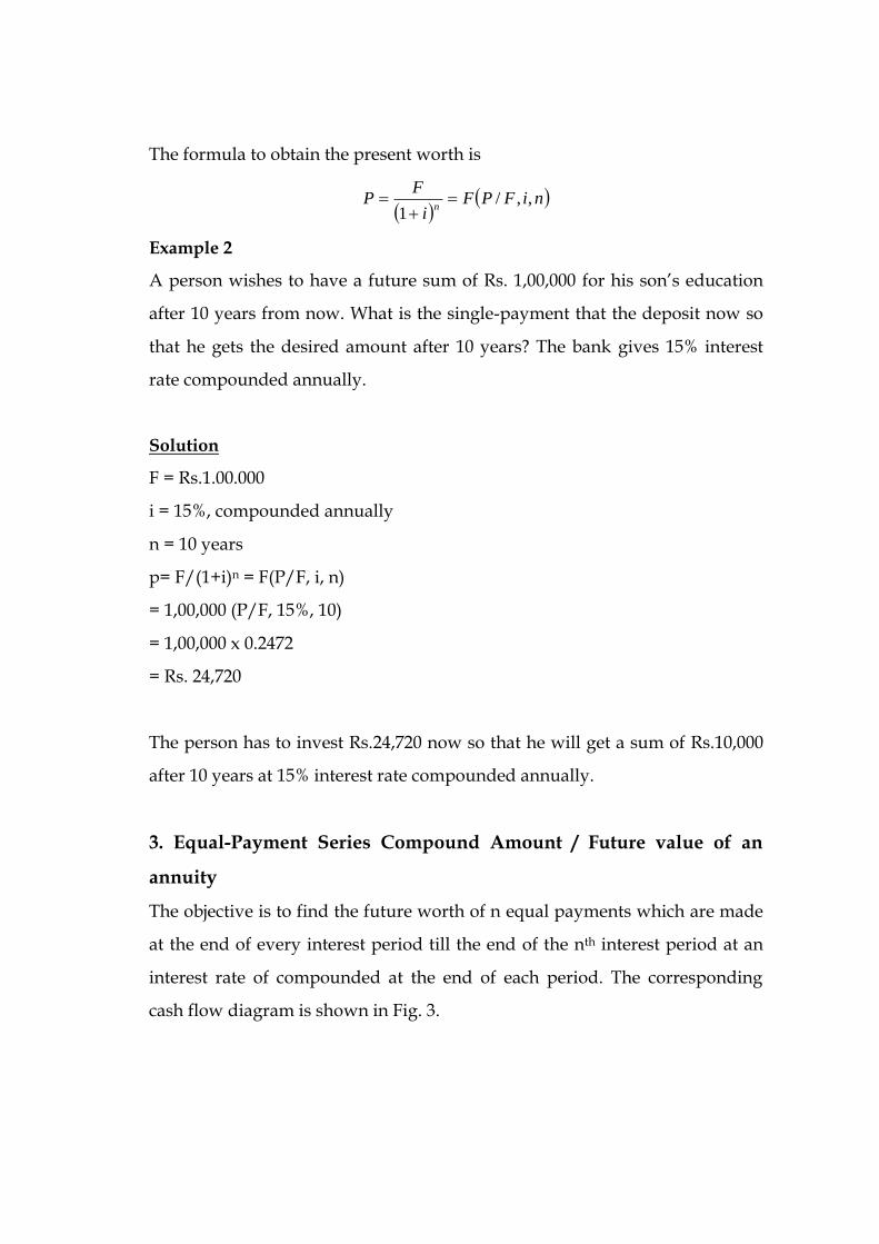
The formula to obtain the present worth is

niFPF

i

FP

n,,/

1

Example 2

A person wishes to have a future sum of Rs. 1,00,000 for his son’s education

after 10 years from now. What is the single-payment that the deposit now so

that he gets the desired amount after 10 years? The bank gives 15% interest

rate compounded annually.

Solution

F = Rs.1.00.000

i = 15%, compounded annually

n = 10 years

p= F/(1+i)n = F(P/F, i, n)

= 1,00,000 (P/F, 15%, 10)

= 1,00,000 x 0.2472

= Rs. 24,720

The person has to invest Rs.24,720 now so that he will get a sum of Rs.10,000

after 10 years at 15% interest rate compounded annually.

3. Equal-Payment Series Compound Amount / Future value of an

annuity

The objective is to find the future worth of n equal payments which are made

at the end of every interest period till the end of the nth interest period at an

interest rate of compounded at the end of each period. The corresponding

cash flow diagram is shown in Fig. 3.

Fig. 3 : Cash flow diagram of equal-payment series compound amount.

Equal amount deposited at the end of each interest period = A

No. of interest periods = n

Rate of interest = i

Single future amount = F

The formula to get F is

niAFA

i

iF

n

A ,,/11

Where (FA,i,n) is termed as equal-payment series compound amount factor.

Example 3 : A person who is not 35 years old is planning for his retired life.

He plans to invest an equal sum of Rs.10,000 at the end of every year for the

next 25 years starting from the end of the next year. The bank gives 20%

interest rate, compounded annually. Find the maturity value of his account

when he is 60 years old.

Solution

A = Rs. 10,000

n = 25 years

i = 20%

F = ?

A A A A - - A

F

1 2 3 4 n

0

1%

The corresponding cash flow diagram is shown below :

Cash flow diagram of equal-payment series compound amount.

F=

i

iA

n11

= A (F/A, i, n)

= 10,000 (F/A, 20%, 25)

= 10,000 x 471.981

= Rs. 47,19,810 The future sum of the annual equal payments after 25 years is

equal to Rs. 47,19,810.

4. Equal-Payment Series Sinking Fund

In this type of investment mode, the objective is to find the equivalent amount

(A) that should be deposited at the end of every interest period for n interest

periods to realize a future sum (F) at the end of the nth interest period at an

interest rate of i

Fig. 4.: Cash flow diagram of equal payment series sinking fund

A = equal amount to be deposited at the end of each interest period

n = No. of interest periods / i = rate of interest

10000 - -

F

1 2 3 4 25

0

10000 10000 10000 10000

i = 20%

A A A A - - A

F

1 2 3 4 n

0

F = single future amount at the end of the nth period

The formula to get F is

niFAF

i

iFA

n,,/

11

where

(A/F, i, n) is called as equal-payment series sinking fund factor.

EXAMPLE

A company has to replace a present facility after 15 years at an outlay of

Rs.5,00,000. It plans to deposit an equal amount at the end of every year for

the next 15 years at an interest rate of 18% compounded annually. Find the

equivalent amount that must be deposited at the end of every year for the

next 15 years.

Solution

F = Rs. 5,00,000

n = 15 years

i = 18%

A= ?

The corresponding cash flow diagram is shown below

Cash flow diagram of equal-payment series sinking fund.

A A A A - - A

F

1 2 3 4 15

0

i =18% 5,00,000

niFAF

i

iFA

n,,/

11

= 5,00,000 (A/F, 18%, 15)

= 5,00,000 X 0.0164

= Rs.8,200

The annual equal amount which must be deposited for 15 years is Rs.8,200.

5. Equal Payment Series Present worth amount

The objective of this mode is investment is to find the present worth of an

equal payment made at the end of every interest period for n interest periods

at interest rate of i compounded at the end of every interest period.

The corresponding cash flow diagram is shown in Fig. 5. Here,

P - present worth

A = annual equivalent payment

i = interest rate

n = No. of interest periods

The formula to compute P is

niAPAii

iAP

n

n

,,/1

11

where (P/A, I, n) is called equal-payment series present worth factor.

Fig. 5 : Cash flow diagram of equal-payment series present worth amount.

A A A A - - A

n

1 2 3 4

P 1%

EXAMPLE 5 : A company wants to set up a reserve which will help company

to have an annual equivalent amount of Rs. 10,00,000 for the next years

towards its employees welfare measures. The reserve is assumed to grow the

rate of 15% annually. Find the single-payment that must be made now the

reserve amount.

Solution

A = Rs.10,00,000

i = 15%

n = 20 years

P = ?

The corresponding cash flow diagram is illustrated below :

Cash flow diagram of equal-payment series present worth amount.

niAPAii

iAP

n

n

,,/1

11

= 10,00,000 X (P/A, 15%, 20)

= 10,00,000 X 6.2593

= Rs.62,59,300

The amount of reserve which must be set-up now is equal to Rs.62,59,300.

10000 - -

20 1 2 3 4 0

10000 10000 10000 10000

i = 10% P

6. Equal-Payment Series Capital Recovery Amount

The objective of this mode of investment is to find the annual equivalent

amount (A) which is to be recovered at the end of every interest period for n

interest periods for a loan (P) which is sanctioned now at an interest rate of i

compounded at the end of every interest period.

Fig. 6 : Cash flow diagram of equal-payment series capital recovery amount.

P - present worth (loan amount)

A = annual equivalent payment (recovery amount)

i = interest rate

n - No. of interest periods

The formula to compute P is as follows:

niPAPi

iiPA

n

n

,,/11

1

where,

(A/P, i, n) is called equal-payment series capital recovery factor.

EXAMPLE 6 A bank gives a loan to a company to purchase an equipment

worth Rs. 10,00,000 at an interest rate of 18% compounded annually. This

amount should be repaid in 15 yearly equal installments. Find the installment

amount that the company has to pay to the bank.

Solution

A A A A - - A

n

1 2 3 4

1% P

P= Rs. 10,00,000

i = 18%

n = 15 years

A - ?

The corresponding cash flow diagram is shown below:

Cash flow diagram of equal-payment series capital recovery amount.

A =

niPAP

i

iiP

n

n

,,/11

1

A) Present Worth Method In all engineering problems the engineers encounter one important

question, i.e., which project to select. To select among the different

alternatives different methods have been evolved. There are several bases for

comparing the worthiness of the projects. Theses bases are

1. Present worth method

2. Future worth method

3. Annual equivalent method

4. Rate of return method

A A A A - - A

15 1 2 3 4

1 = 18% P

1000000

5. Pay back period

Present worth method is one of them. Many economists prefer a present

worth analysis because it reveals the sum in today’s rupee that is equivalent

to a future cash flow stream. For example – Rs.110/- expected one year hence

is worth only Rs.100/- today, if the rate of interest is 10%, compounded

annually. This means that Rs.100/- is the present value of Rs.110/- to be

earned one year hence.

Under this method, the present worth of all cash inflows (revenues) is

compared against the present worth of all cash outflows (costs) associated

with an investment project. In this method of comparison, the cash flow of

each alternative will be reduced to time zero by assuming an interest rate i.

Then, depending on the type of decision, the best alternative will be selected

by comparing the present worth amounts of the alternatives. The difference

between the present worth of the cash flows (inflows – outflows) referred to

as the Net Present Worth. NPW determines whether or not the project is an

acceptable investment.

Conditions for Present worth Comparison

(i) Estimate the interest rate that the firm wishes to earn on its

investment.

(ii) Determine the service life of the project.

(iii) Determine the cash inflows over each service life.

(iv) Determine the cash overflows over each service period.

(v) Estimate the net cash flows (inflows – outflows).

If there is single investment proposal, whether a project will be selected or

rejected that can be made accordingly.

If PW > 0, select the proposal. A positive NPW means the equivalent

worth of the inflows is greater than the equivalent worth of outflows. So, the

project makes profit.

If PW < 0, reject the investment project. A negative NPW means the

equivalent worth of the inflows is less than the equivalent worth of outflows.

If PW = 0, remain indifferent to the investment.

If we have mutually exclusive alternatives then present worth cash flows can

be calculated by two prominent methods. These are

(i) Revenue based present worth

(ii) Cost based present worth.

In a revenue/ profit dominated cash flow diagram, the profit, revenue,

salvage value (all inflows to an organization) will be assigned with positive

sign. The costs (out flows) will be assigned with negative sign.

In a cost dominated cash flow diagram the costs (out flows) will be

assigned with positive sign and the profit, revenue, salvage value (all inflows)

etc. will be assigned with negative sign. In case the decision is to select the

alternative with the maximum profit, then the alternative with the maximum

present worth will be selected.

If the decision is to select the alternative with the minimum cost, then

the alternative with the least present worth amount will be selected.

Revenue dominated cash flow diagram

S

R1 R2 R3 Rn

0 1 2 3 n

P

Where ‘P’ is the initial investment

‘Rn’ is the net revenue at the end of nth year.

‘i’ is the interest rate compounded annually

‘S’ is the salvage value at the end of the nth year.

To find the present worth of the cash flow from the above diagram for a given

interest rate, the formula is

nn

n

i

S

i

R

i

R

i

RPiPW

)1()1(......

)1()1()(

2

2

1

1

Or

PW(i) = -P + R1(P/F,i,1) + R2(P/F, i, 2) + …….+ Rn(P/F, i,n) + S(P/F, i,n)

If it is a uniform series or equal payment series then the formula will be

PW(i) = -P + R (P/F, i, n) + S (P/F, i, n)

Cost dominated cash flow diagram

S 0 1 2 3 4 5 P C1 C2 C3 C4 C5 Cn

Where ‘P’ is the initial investment

‘Cn’ is the net cost of operation and maintenance at the end of the nth

year

‘S’ is the salvage value at the end of the nth year

‘Ci’ is the discounted rate of interest

and for it the present worth expression is

nn

n

i

S

i

C

i

C

i

CPiPW

)1()1(......

)1()1()(

2

2

1

1

Or

PW(i) = -P + C1(P/F,i,1) + C2(P/F, i, 2) + …….+ Cn(P/F, i,n) - S(P/F, i,n)

It is a uniform series or equal payment series then the formula will be

PW(i) = P + C (P/F, i, n) - S (P/F, i, n)

Examples

In this section, the concept of present worth method of comparison

applied to the selection of the best alternative is demonstrated with several

illustrations.

Example 1 : the following table summarizes a cash flow stream of an

investment project.

Year (n) Net cash flows (Rs.)

0

1

2

3

4

-6,50,000

1,62,500

1,62,500

1,62,500

….

5

6

7

8

….

….

….

1,62,500

If the firm’s rate of interest is 15%, compute the NPW of this project. Is this

project acceptable ?

Solution : The cash flow diagram for the given project is A = Rs.1,62,500

0 1 2 3 4 …………………. 8 Rs. 6,50,000 Year This is a uniform cash flow stream. Since the project requires an initial

investment of Rs. 6,50,000 at present (n = 0) followed by 8 equal annual

receipt of Rs. 1,62,500, we can easily determine the NPW as follows :

NPW = -P + R ( P/A, i,n )

= - Rs. 6,50,000 + Rs. 1,62,500 (P/A, 15%, 8)

= - Rs. 6,50,000 + Rs. 1,62,500 (4.4873)

= - Rs. 6,50,000 + Rs. 7,92,190

= Rs. 79,190

Since, PW (15%) > 0, the project would be acceptable.

Example 2 : The project cash flows of an investment proposal is given below.

End of Year Net cash flows (Rs.)

0

1

-50,000

20,400

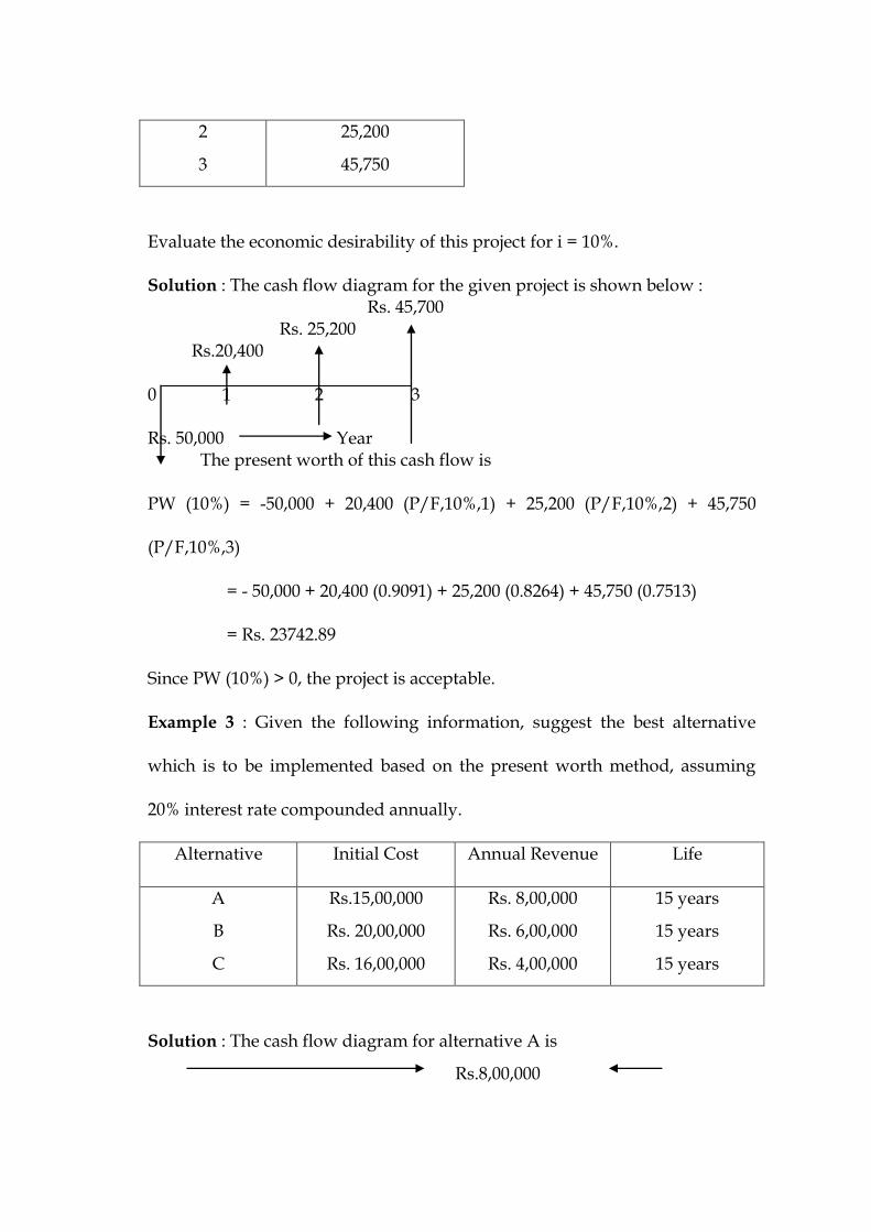
2

3

25,200

45,750

Evaluate the economic desirability of this project for i = 10%.

Solution : The cash flow diagram for the given project is shown below : Rs. 45,700 Rs. 25,200 Rs.20,400 0 1 2 3 Rs. 50,000 Year The present worth of this cash flow is

PW (10%) = -50,000 + 20,400 (P/F,10%,1) + 25,200 (P/F,10%,2) + 45,750

(P/F,10%,3)

= - 50,000 + 20,400 (0.9091) + 25,200 (0.8264) + 45,750 (0.7513)

= Rs. 23742.89

Since PW (10%) > 0, the project is acceptable.

Example 3 : Given the following information, suggest the best alternative

which is to be implemented based on the present worth method, assuming

20% interest rate compounded annually.

Alternative Initial Cost Annual Revenue Life

A

B

C

Rs.15,00,000

Rs. 20,00,000

Rs. 16,00,000

Rs. 8,00,000

Rs. 6,00,000

Rs. 4,00,000

15 years

15 years

15 years

Solution : The cash flow diagram for alternative A is

Rs.8,00,000

0 1 2 3 …………. 14 15

Rs. 15,00,000 Year

The present worth for this cash flow is

PW(20%)A = - Rs. 15,00,000 + Rs. 8,00,000 (P/A,20%,15)

= - Rs. 15,00,000 + Rs. 8,00,000 (4.6755)

= Rs. 22,40,400

The cash flow diagram for alternative B is

Rs.6,00,000

0 1 2 3 …………. 14 15

Rs. 20,00,000 Year

PW(20%)B = - Rs. 20,00,000 + Rs. 6,00,000 (P/A,20%,15)

= - Rs. 20,00,000 + Rs. 6,00,000 (4.6755)

= Rs. 8,05,300

The cash flow diagram of alternative C is

Rs.4,00,000

0 1 2 3 …………. 14 15

Rs. 16,00,000 Year

PW(20%)C = - Rs. 16,00,000 + Rs. 4,00,000 (P/A,20%,15)

= - Rs. 16,00,000 + Rs. 4,00,000 (4.6755)

= Rs. 2,70,200

Since the present worth of alternative A is the highest among all the

alternatives so it is suggested for implementation.

Example 4 : Given the following information, suggest which technology

should be selected based on present worth method, assuming 15% interest

rate compounded annually.

Technology Initial Cost (Rs.) Service Life Annual O & M

Cost

A

B

4,00,000

5,00,000

15 Years

15 Years

25,000

29,000

Solution : The cash flow diagram of technology A is

0 1 2 3 …………. 14 15

Rs. 25,000

Rs. 4,00,000

The present worth amount of this cash flow stream is

PW(15%)A = Rs. 4,00,000 + Rs. 25,000 (P/A,15%,15)

= Rs. 4,00,000 + Rs. 25,000 (5.8474)

= Rs. 4,00,000 + Rs. 1,46,185

= Rs. 5,46,185

The cash flow diagram for technology B is

0 1 2 3 …………. 14 15

Rs. 29,000

Rs. 5,00,000

PW(15%)B = Rs. 5,00,000 + Rs. 29,000 (P/A, 15%, 15)

= Rs. 5,00,000 + Rs. 29,000 (5.8474)

= Rs. 5,00,000 + Rs. 1,69,574.6

= Rs. 6,69,574.6

Since PW amount of technology A is lower, hence technology A is to be

selected.

Example 5 : A finance company advertises two investment plans. In plan 1 the

company pays Rs. 22,000 after 15 years for every Rs.1,000 invested now. In

plan 2, for every Rs. 1,000 invested the company pays Rs. 4,000 at the end of

the 10th year and Rs. 4,000 at the end of 15th year. Select the best investment

plan at i = 10% compounded annually.

Solution :

Plan 1 : Cash flow diagram for plan 1 is

The cash flow diagram of alternative C is

Rs.22,000

0 1 2 3 ……………………………………… 15

i = 10%

B) FUTURE WORTH METHOD Future worth method is particularly useful in an investment situation

where we need to compute the equivalent worth of a project at the end of its

investment period rather than at its beginning.

Conditions for computing Future Worth Method

1. Determine the interest rate

2. Estimate the service life of the project

3. Estimate the cash inflows for each period over the service life.

4. Estimate the cash outflows over each service period.

5. Determine the net cash flows (inflows – outflows).

For a single project evaluation

If FW > 0, project is accepted.

If FW < 0, reject the investment proposal.

If FW = 0, remain indifferent to the investment.

For a mutually exclusive alternatives future worth cash flows can be

calculated by

i) Revenue based future worth

ii) Cost based future worth.

In revenue based cases the alternative with maximum future worth amount

will be selected. In cost based cases the alternative with the least future worth

amount will be accepted.

The formula for the future worth for a given interest rate i is

FW(i) = - P(1 + i)n + R1(1 + i)n-1 + R2(1 + i)n-2 + ………..+ Rn + S

Or

FW(i) = - P(F/P, i,n) + R1(F/P, i, n-1) + R2(F/P, i, n-2) + ……….+ Rn + S

If it is equal payment series then the formula will be

FW(i) = - P(F/P, i,n) + R (F/P, i, n) + S

In these cases the alternative with the maximum future worth amount should

be selected as the best alternative.

If the cash flow stream is cost-based, then the future worth is given by

FW(i) = P(1 + i)n + C1(1 + i)n-1 + C2(1 + i)n-2 + ………..+ Cn – S

Or

(C) EQUIVALENT ANNUAL WORTH COMPARISON

(EAW)

There are various alternatives for comparing the worthiness of a project

Equivalent Annual Worth (EAW) is one important method for comparing

engineering alternatives. In an annual worth method, all the receipts and

disbursements occurring over a period are converted to an equivalent

uniform yearly amount. EAW is a popular method because of a year’s profit

and losses are taken into account. A large number of engineering economic

decisions are based on annual comparison and so the term equivalent

uniform yearly amount often used. For example, cost accounting procedures,

depreciation charges, tax calculations etc. These yearly cost tabulations

generally make the annual worth method easier.

Equivalent Annual Cost (EAC) indicates that the equivalent value of negative

cash flow for disbursement is greatly than the corresponding positive flow of

receipts.

Diagram of EAW

We will use the term equivalent annual worth (EAW) when costs and receipts

are both present.

0

R1 R2

R3

Rn

C1 C2 C3

Cn Cost

R

ecei

pt

Years n

……

…. ……

….

Diagram of EAC

We will use the term equivalent annual cost (EAC) to designate comparison

involving only costs.

Conditions for Computing EAW

1. Estimate the cash flows (inflows, outflows) over each service period.

2. Estimate the service life of the project.

3. Determine the interest rate.

4. Comparisons are made with before-tax cash flows.

5. EAW comparisons do not include intangible considerations.

For single alternatives if

EAW > 0, Accept the investment proposal

EAQ < 0, Reject the investment proposal

EAW = 0, Remain indifferent to the investment.

For multiple alternatives or mutually exclusive alternatives if all the

alternatives are revenue dominated, the all the alternatives are revenue

dominated, the alternative with higher EAW will be selected. If all the

alternatives are cost based, the alternatives with least EAW will be accepted.

EAW consists of following steps

i. complete the net present worth (NPW)

0

C1

Cost

s R

ecei

pt

s

C2 C3 C4 Cn

Year

s

1 2 3 4 n …….

ii. Multiply the amount of present worth by the capital recovery factor. i.e.

EAW = PW(i) (A/P, i, n) where (A/P, i,n) is called equal-payment series

capital recovery factor .

The annual equivalent worth can be computed by using the general formula.

i.e.,

11

1)(

n

n

i

iiiPWEAW

Example 1

Consider a machine that costs Rs.40,000 and a 10 year useful life. At the end of

10 year, it can be sold for Rs.5,000 after tax adjustment. If the firm could earn

an after-tax revenue of Rs.10,000 per year with this machine, should it be

purchased at an interest rate of 15%, compounded annually.

Solution

Initial cost (P) – Rs.40,000/-

Useful life (n) – 10 years

Salvage value - Rs. 5,000/-

Revenue – Rs.10,000/-

i = 15%, compound annually

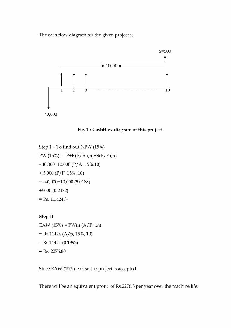
40,000

2 1 3 10

S=500

0

…………………………………

…………

The cash flow diagram for the given project is

Fig. 1 : Cashflow diagram of this project

Step 1 – To find out NPW (15%)

PW (15%) = -P+R(P/A,i,n)+S(P/F,i,n)

- 40,000+10,000 (P/A, 15%,10)

+ 5,000 (P/F, 15%, 10)

= -40,000+10,000 (5.0188)

+5000 (0.2472)

= Rs. 11,424/-

Step II

EAW (15%) = PW(i) (A/P, i,n)

= Rs.11424 (A/p, 15%, 10)

= Rs.11424 (0.1993)

= Rs. 2276.80

Since EAW (15%) > 0, so the project is accepted

There will be an equivalent profit of Rs.2276.8 per year over the machine life.

10000

D. RATES OF RETURN METHOD

The rate of return is a percentage that indicates the relative yield on different

uses of capital. Three rates of return appear frequently in engineering

economy studies:

The minimum acceptable rate of return (MARR) is the rate set by an

organization to designate the lowest level of return that makes an investment

acceptable.

The internal rate of return (IRR) is the rate on the unrecovered balance of the

investment in a situation where the terminal balance is zero. It is a discount

rate at which NPV = 0.

The external rate of return (ERR) is the rate of return that is possible to obtain

for an investment under current economic conditions. For example, suppose

that analysis of an investment shows that it will realize an IRR of 50 percent.

Rationally, it is not reasonable to expect that we can invest in the external

market and get that high a rate. In engineering economy studies, the external

interest rate most often will be set to the MARR.

MINIMUM ACCEPTABLE RATE OF RETURN

The minimum acceptable rate of return, also known as the minimum

attractive rate of return, is a lower limit for investment acceptability set by

organizations or individuals. It is a device designed to make the best possible

use of a limited resource, i.e., money. Rates vary widely according to the type

of organization, and they vary even within the organization. Historically,

government agencies and regulated public utilities have utilized lower

required rates of return than have 'competitive industrial enterprises. Within

a given enterprise, the required rate may be different for various divisions or

activities. These variations usually reflect the risk involved. For instance, the

rate of return required for cost reduction proposals may be lower than that

required for research and development projects in which there is less certainty

about prospective cash flows.

INTERNAL RATE OF RETURN

The IRR is the best-known and most widely used rate-of-return method. It is

also known as the true rate-of-return method and the discounted cash flow

method. The internal rate of return, represented by i in the traditional

interpretation of interest rates, is the rate of interest earned by an alternative

investment on the unrecovered balance of an investment.

The internal rate of return can be calculated by equating the annual, present,

or future worth of cash flow to zero and solving for the interest rate (IRR) that

allows the equality, it should be added that solving for the interest rate in this

manner results in a polynomial equation that is a function of i, which may

result in multiple roots of the equation (). In such cases the IRR may or may

not be one of the equation roots.

Although both the EAW and FW approaches are legitimate, the rate of return

is often defined in terms of present worth, under the constraints of possible i*

roots, where the IRR is

The interest rate at which the present worth of the cash flow of a project is zero,

or, to restate this in another way:

The rate which when employed in computing the present worth of all costs and

present worths of all returns will make them equal

Because rate-of-return computations usually begin with a problem expressed

in terms of present worth or annual worth, it is necessary to pay attention to

the guidelines for the EAW and PW methods. In particular, mutually

exclusive alternatives (where selection of one precludes selection of others)

must be compared on the basis of equivalent outcomes. In the case of

independent alternatives (the choice of one does not affect the choice of

another, except for limited capital availability), all costs and benefits must be

explicitly stated.

Calculation of IRR

Determining the IRR is a function of the type of investment (simple, pure, and

mixed) and the characteristics of the alternatives (mutually exclusive or

independent). If we have independent projects, we may fund combinations of

the projects since an independent project does not affect the funding of

another project (except for capital availability limitations which are very real

in most situations analyzed by the engineering economist). The cash flows of

several independent alternatives that are being considered as a group may be

summed to form the group's composite cash flow. Analysis can then be

performed on this composite cash flow. Where capital limitations are

apparent in a department and several independent alternatives are competing

for funding, combinations of alternatives may be formed where each

combination's first costs have to be equal to or less than the capital available.

In this case, mutually exclusive combinations will usually be realized, where

selection of one group of independent alternatives will preclude the selection

of another. This can be due to alternatives being in more than one group

and/or capital limitations.

We will see that ranking alternatives according to their IRR values is not

consistent with the PW, FW, or AW rankings. Mutually exclusive alternatives

may be analyzed by incremental IRR analysis, and the results will be found to

be completely consistent with the PW, FW, and AW methods. Incremental

analysis assumes that we start with a satisfactory low-investment alternative.

Analysis of a higher-investment alternative is then based on the differences

between the cash flows of the second alternative and the acceptable

alternative. These differences in cash flows are incremental cash flows. The

cash flow of the second alternative is equal to the cash flow of the first

alternative plus the incremental cash flows. Thus, if the incremental cash flow

is acceptable when compared to the MARR, then the larger investment has to

be a better investment than the first alternative, which was also acceptable.

Otherwise, remove the larger investment from consideration. This type of

evaluation is continued until all alternatives have been evaluated; one of the

mutually exclusive alternatives is then determined to be the best investment.

As mentioned earlier, there is a possibility that the PW equation may be a

polynomial in terms of i such that multiple roots i* of polynomial PW(i') may

result. Often, multiple i*'s are assumed to be multiple IRR values. This is

misleading since there is really only one true IRR for an investment, and so

we will need to determine which i*, if any, is the investment IRR. Classifying

investments into simple and nonsimple investments will tell us if just one i*

exists which, in turn, tells us that we have found the IRR when we have found

i*. An investment is simple if there is only one cash flow sign change (minus

to plus) from period to period.:

D. RATES OF RETURN METHOD

The rate of return is a percentage that indicates the relative yield on different

uses of capital. Three rates of return appear frequently in engineering

economy studies:

The minimum acceptable rate of return (MARR) is the rate set by an

organization to designate the lowest level of return that makes an investment

acceptable.

The internal rate of return (IRR) is the rate on the unrecovered balance of the

investment in a situation where the terminal balance is zero. It is a discount

rate at which NPV = 0.

The external rate of return (ERR) is the rate of return that is possible to obtain

for an investment under current economic conditions. For example, suppose

that analysis of an investment shows that it will realize an IRR of 50 percent.

Rationally, it is not reasonable to expect that we can invest in the external

market and get that high a rate. In engineering economy studies, the external

interest rate most often will be set to the MARR.

MINIMUM ACCEPTABLE RATE OF RETURN

The minimum acceptable rate of return, also known as the minimum

attractive rate of return, is a lower limit for investment acceptability set by

organizations or individuals. It is a device designed to make the best possible

use of a limited resource, i.e., money. Rates vary widely according to the type

of organization, and they vary even within the organization. Historically,

government agencies and regulated public utilities have utilized lower

required rates of return than have 'competitive industrial enterprises. Within

a given enterprise, the required rate may be different for various divisions or

activities. These variations usually reflect the risk involved. For instance, the

rate of return required for cost reduction proposals may be lower than that

required for research and development projects in which there is less certainty

about prospective cash flows.

INTERNAL RATE OF RETURN

The IRR is the best-known and most widely used rate-of-return method. It is

also known as the true rate-of-return method and the discounted cash flow

method. The internal rate of return, represented by i in the traditional

interpretation of interest rates, is the rate of interest earned by an alternative

investment on the unrecovered balance of an investment.

The internal rate of return can be calculated by equating the annual, present,

or future worth of cash flow to zero and solving for the interest rate (IRR) that

allows the equality, it should be added that solving for the interest rate in this

manner results in a polynomial equation that is a function of i, which may

result in multiple roots of the equation (). In such cases the IRR may or may

not be one of the equation roots.

Although both the EAW and FW approaches are legitimate, the rate of return

is often defined in terms of present worth, under the constraints of possible i*

roots, where the IRR is

The interest rate at which the present worth of the cash flow of a project is zero,

or, to restate this in another way:

The rate which when employed in computing the present worth of all costs and

present worths of all returns will make them equal

Because rate-of-return computations usually begin with a problem expressed

in terms of present worth or annual worth, it is necessary to pay attention to

the guidelines for the EAW and PW methods. In particular, mutually

exclusive alternatives (where selection of one precludes selection of others)

must be compared on the basis of equivalent outcomes. In the case of

independent alternatives (the choice of one does not affect the choice of

another, except for limited capital availability), all costs and benefits must be

explicitly stated.

Calculation of IRR

Determining the IRR is a function of the type of investment (simple, pure, and

mixed) and the characteristics of the alternatives (mutually exclusive or

independent). If we have independent projects, we may fund combinations of

the projects since an independent project does not affect the funding of

another project (except for capital availability limitations which are very real

in most situations analyzed by the engineering economist). The cash flows of

several independent alternatives that are being considered as a group may be

summed to form the group's composite cash flow. Analysis can then be

performed on this composite cash flow. Where capital limitations are

apparent in a department and several independent alternatives are competing

for funding, combinations of alternatives may be formed where each

combination's first costs have to be equal to or less than the capital available.

In this case, mutually exclusive combinations will usually be realized, where

selection of one group of independent alternatives will preclude the selection

of another. This can be due to alternatives being in more than one group

and/or capital limitations.

We will see that ranking alternatives according to their IRR values is not

consistent with the PW, FW, or AW rankings. Mutually exclusive alternatives

may be analyzed by incremental IRR analysis, and the results will be found to

be completely consistent with the PW, FW, and AW methods. Incremental

analysis assumes that we start with a satisfactory low-investment alternative.

Analysis of a higher-investment alternative is then based on the differences

between the cash flows of the second alternative and the acceptable

alternative. These differences in cash flows are incremental cash flows. The

cash flow of the second alternative is equal to the cash flow of the first

alternative plus the incremental cash flows. Thus, if the incremental cash flow

is acceptable when compared to the MARR, then the larger investment has to

be a better investment than the first alternative, which was also acceptable.

Otherwise, remove the larger investment from consideration. This type of

evaluation is continued until all alternatives have been evaluated; one of the

mutually exclusive alternatives is then determined to be the best investment.

As mentioned earlier, there is a possibility that the PW equation may be a

polynomial in terms of i such that multiple roots i* of polynomial PW(i') may

result. Often, multiple i*'s are assumed to be multiple IRR values. This is

misleading since there is really only one true IRR for an investment, and so

we will need to determine which i*, if any, is the investment IRR. Classifying

investments into simple and nonsimple investments will tell us if just one i*

exists which, in turn, tells us that we have found the IRR when we have found

i*. An investment is simple if there is only one cash flow sign change (minus

to plus) from period to period. A simple investment is as follows:

Time period Cash flow (Rs.) Sign change

Cost Benefit Analysis

The question to which cost benefit analysis addresses itself is whether it is

socially desirable to undertake a number of investment project A, B, C, D etc,

and if investible funds are limited, then how many of these should be

selected. Since the choice involves maximization, we have to discuss what it is

that investment planners wish to maximize. In general terms an investment

planners wants to maximize the present value of all benefits less that of all

costs, subject to specific constraints. This general formulation raises the

following specific questions, the answer to which provide the general

principles of cost benefit analysis.

• In project appraisal which costs and which benefits are to be

considered?

• How are these costs and benefits to be valued?

• How can profitability of a project be measured?

• What is the relevance of uncertainty in project appraisal?

• What are the relevant constraints?

There is certainty some arbitrariness in the choice of these questions.

In evaluating alternatives of private organizations, the criterion is to select the

alternative with the maximum profit. The profit maximization is the main

goal of private organizations while providing goods/services as per

specifications to their customers. But the same criterion cannot be used while

Time period Cash flow (Rs.) Sign change

evaluating public alternatives. Examples of some public alternatives are

constructing bridges, roads, dams, establishing public utilities, etc.

The main objective of any public alternative is to provide goods/services to

the public at the minimum cost. In this process, one should see whether the

benefits of the public activity are at least equal to its costs. If yes, then the

public activity can be undertaken for implementation. Otherwise, it can be

cancelled. This is nothing but taking a decision based on Benefit-Cost ratio

(BC) given by

The benefits may occur at different time periods of the public activity. For the

purpose of comparison, these are to be converted into a common time base

(present worth or future worth or annual equivalent). Similarly, the costs

consist of initial investment and yearly operation and maintenance cost. These

are to be converted to a common time base as done in the equivalent benefits.

Now the ratio between the equivalent benefits and equivalent costs is known

as the “Benefit-Cost ratio”. If this ratio is at least one, the public activity is

justified; otherwise, it is not justified. Let

BP - present worth of the total benefits

BF = future worth of the total benefits

BA = annual equivalent of the total benefits

P = initial investment

PF = future worth of the initial investment

PA = annual equivalent of the initial investment

C = yearly cost of operation and maintenance

CP = present worth of yearly cost of operation and maintenance

CF - future worth of yearly cost of operation and maintenance

EXAMPLES 1.1

EXAMPLE-1 In a particular locality of a state, the vehicle users take a

roundabout route to reach certain places because of the presence of a river.

This results in excessive travel time and increased fuel cost. So, the state

government is planning to construct a bridge across the river. The estimated

initial investment for constructing the bridge is Rs. 40,00,000. The estimated

life of the bridge is 15 years. The annual operation and maintenance cost is Rs.

1,50,000. The value of fuel savings due to the construction of the bridge is Rs.

6,00,000 in the first year and it increases by Rs. 50,000 every year thereafter till

the end of the life of the bridge. Check whether the project is justified based

on BC ratio by assuming an interest rate of 12%, compounded annually.

Solution

Initial investment = Rs. 40,00,000

Annual operation and maintenance = Rs. 1,50,000

Annual fuel savings during the first year = Rs. 6,00,000

Equal increment in fuel savings in the following years = Rs. 50,000

Life of the project = 15 years

Interest rate = 12%

6,00,000 + 7,00,000

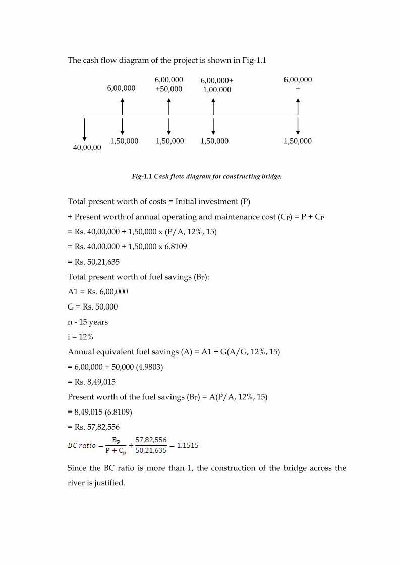
The cash flow diagram of the project is shown in Fig-1.1

Fig-1.1 Cash flow diagram for constructing bridge.

Total present worth of costs = Initial investment (P)

+ Present worth of annual operating and maintenance cost (CP) = P + CP

= Rs. 40,00,000 + 1,50,000 x (P/A, 12%, 15)

= Rs. 40,00,000 + 1,50,000 x 6.8109

= Rs. 50,21,635

Total present worth of fuel savings (BP):

A1 = Rs. 6,00,000

G = Rs. 50,000

n - 15 years

i = 12%

Annual equivalent fuel savings (A) = A1 + G(A/G, 12%, 15)

= 6,00,000 + 50,000 (4.9803)

= Rs. 8,49,015

Present worth of the fuel savings (BP) = A(P/A, 12%, 15)

= 8,49,015 (6.8109)

= Rs. 57,82,556

Since the BC ratio is more than 1, the construction of the bridge across the

river is justified.

6,00,000 6,00,000

+50,000

6,00,000+

1,00,000

6,00,000

+

7,00,000

40,00,00

0

1,50,000 1,50,000 1,50,000 1,50,000

DEPRECIATION ANALYSIS

Depreciation is the decrease in value of physical properties with the passage

of time and use. Most assets are worthless as they age. Production equipment

gradually becomes less valuable through wear and tear. This lessening in

value is recognised in accounting practices as an operating expense. Instead of

charging the full purchase price of a new asset as one time expense, the outlay

is spread over the life of the asset in the accounting records. Annual

depreciation deductions arc intended to match the yearly fraction of value

used by an asset in the production of income over the assets actual economic

life. The actual amount of depreciation can never be established until the asset

is retired from service.

Depreciation can be defined in three senses like physical depreciation, which

is caused due to physical decay. Economic depreciation is the loss of value of

an asset due to outdated technology and in accounting sense depreciation is

the estimated value of fall in the worth of an asset. In accounting, depreciation

charge is included in the cost of production of the asset. Depreciation is a

permanent continuing and gradual shrinkage in the book value of a fixed

asset.

Causes of depreciation:

Assets depreciate its value for several reasons.

1. Physical depreciation

Depreciation resulting in physical impairment of an asset is known as

physical depreciation. This type of depreciation results in the lowering of the

ability of a physical asset to render its intended service. The primary causes of

physical depreciation are (a) deterioration due to action of the elements

including the corrosion of pipe, the rotting of timbers, chemical

decomposition and so on. (b) Wear and tear charges (c) Physical decay, (d)

Time factors etc.

2. Functional depreciation

Functional depreciation results not from a deterioration in the assets ability to

serve its intended purpose, but from a change in the demand for the services

it can render. The demand for the services of an asset may change it is more

profitable to use a more efficient, unit, there is no longer work for the asset to

do, or the work to he done exceeds the capacity of the asset.

3. Technological depreciation

Due to advancement of new technology, the old technology becomes

outdated, so it loses its value. Obsolescence resulting from the discovery of

another asset that is sufficiently superior to make it uneconomical to continue

using the original asset. Assets also become obsolete when they are no longer

needed.

4. Depreciation due to accident

Sometimes due to accident or sudden failure the asset loses its technological

characteristic inherent in it.

5. Depreciation due to depletion

Consumption of an exhaustible natural resources to produce product or

services is termed as depletion. Removal of oil, timber, rock or minerals from

a site decreases the value of the holding. This decrease is compensated by a

proportionate reduction in earnings derived from the resources.

6. Monetary depreciation

A change in the price level also decreases the value of owned assets. If prices

rise during the life of an asset, then comparable replacement become more

expensive. This means that the capital recovered will be insufficient to

provide an adequate substitute for the worn out asset.

7. Depreciation due to time factor

There are some assets, which loses its values after a particular time period.

Particularly the assets having lease, copyrights and patents right loses its

value after the time is over.

8. Depreciation due to deferred maintenance

Sometimes the loss of value of asset begin very quickly due to deferred

maintenance. If proper materials are not used or instructions to operate the

machine are not properly obeyed the loss of value start.

9. Depreciation Accounting

Before going through the different method involved in the calculation of

depreciation we should have sufficient knowledge about the depreciable

property. Depreciable property is that property which can amortized or

depreciated. Depreciable property may be tangible and intangible. Tangible

property is any property that can be seen or touched. Intangible property are

property which are not tangible like copyrights and patent rights. Depreciable

tangible property is of two types i.e. Real and personal. Personal property are

those property which is not real estate, they are machinery and equipments.

Real property is land and anything that is erected on. Land is never

depreciable.

Property is depreciable if it fulfills the following requirements:

a) The property must be used in business or help to produce income

b) The property must be something that wears out, decays, deteriorates,

becomes obsolete, or loses value from natural causes.

c) It must have determinable life and that life must be longer than 1 year.

In general, if property does not fulfill the above conditions can’t be regarded

as depreciable property.

Depreciation Methods

There are various depreciation method have evolved form time to time but

there are three basic methods to understand the various calculation of

depreciation schedules that are presently, in effect, it is first necessary to

become acquainted with the three methods on which the current schedules

are based. Some current depreciation schedules are based on straight line

depreciation and other are based on a combination of straight line

depreciation and declining balance depreciation.

Before going to discuss the basic methods and other methods of depreciation

we should know some additional terms for clear understanding of the

problem.

P = Purchase price (unadjusted basis) of assets. (This is the initial cost of

occurring an asset (purchase price + sales taxes) including transportation

expenses.

S= Salvage value or future value at end of asset’s life. It is the expected selling

price of a property when the asset can no longer be used by its owner.

N = useful (tax) life of asset - The expected period of time that a property will

be used in a trade or business or to produce income.

N = number of years of depreciation

Dt (n) = Annual depreciation charges.

Bt(n) = Book value shown on accounting records at end of year. It is the

original cost, basis of the property, including any adjustment.

Bt(0)=p

Straight line method

The most widely used and simplest method for the calculation of depreciation

is straight line method. The straight line method assumes that the value of an

asset decrease at a constant rate. Thus if an asset has a first cost of Rs.5,000

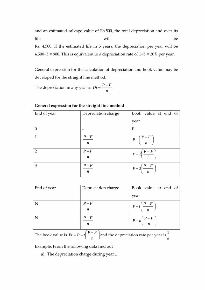
and an estimated salvage value of Rs.500, the total depreciation and over its

life will be

Rs. 4,500. If the estimated life in 5 years, the depreciation per year will be

4,5005 = 900. This is equivalent to a depreciation rate of 15 = 20% per year.

General expression for the calculation of depreciation and hook value may be

developed for the straight line method.

The depreciation in any year is n

FPDt

General expression for the straight line method

End of year Depreciation charge Book value at end of

year

0 - P

1

n

FP

n

FPP

2

n

FP

n

FPP 2

3

n

FP

n

FPP 3

End of year Depreciation charge Book value at end of

year

N

n

FP

n

FPtP

N

n

FP

n

FPnP

The book value is

n

FPtPBt and the depreciation rate per year is

n

1

Example: From the following data find out

a) The depreciation charge during year 1

b) The depreciation charge during year 2

c) The depreciation reserve accumulated by the end of year 3

d) The book value at the end of year 3

Initial con of the asset = Rs. 5000

Life time = 5 years

Salvage value = 0

The cost of capital 5%

Solution

(a) &. (b) In case of straight line method as the depreciation charge is constant,

the depreciation charges for year 1 and 2 is constant.

5

5000)2()1(

n

FPDtDt = 1000 per year

(c) The depreciation reserve at the end of the third year is the sum of the

annual depreciation charges for the first three years and is equal to 3 (1000) =

Rs. 3000

(d) The book value at the end of third year is = 20005

500035000

Bt (3) = 5000- 3000 = Rs. 2000

Declining balance Method

Value of an asset diminishes at a decreasing rate. The declining balance

depreciation assumes that an asset decreases in value-faster early rather than

in the latter portion of its service life. By this method a fixed percentage is

multiplied times the book value the asset at the beginning of the year to

determine the depreciation charge for that year. Thus as the book value of the

asset decreases through time, so does the size of the depreciation charge.

For example - First cost Rs. 5,000 Salvage value =Rs.l000

life of the asset five year, Depreciation rate 30% per year.

Declining Balance method

End of year Depreciation charge during year

Bank value at end of year Rs.

0 5000

1 (0.30) (50000) = 1,500 3,1500

2 (0.30) (3,500) = 1,050 2,450

3 (0.30) (2,450) = 735 1,715

4 (0.30) (1,7115) = 515 1,200

5 (0.30) (1,200) = 360 840

For a depreciation rate a, the general relationship expressing the depreciation

charge in any year for declining balance depreciation is:

D(t)= a.BV(t-1)

We know book value

BV(t)= Bt-1 – Dt

Therefore, declining-balance depreciation.

B(t)= Bt-1 – a.Bt-1

Using this recursive expression, we can determine the general expression for

the depreciation charge and the book value for any point of time. These

calculations are shown in the table.

D(t) = a(1-a)t-1 P

and the book value BV(t) = (1 - R) P

BV(t) = P(1-a)t

General expression for the declining balance method of depreciation

End of year

Depreciation charge during year

Book value at end of year

0 - P

1 a x B0 = a (P) (1-a) B0 = (1-a) P

2 a x B1 = a (1-R) P (1-a) B1 = (1-a)2 P

3 a x B2 = a (1-R)2 P (1-a) B2 = (1-a)3 P

T a x Bt-1 = a (1-R)t-1 P (1-a) Bt-1 = (1-a)t P

N a x Bt-1 = a (1-R)n-1 P (1-a) Bn-1 = (1-a)n P

If the declining balance method of depreciation is used for income tax

purposes the maximum rate that may be used is double the straight line rate

that would be allowed to a particular asset a group of asset being depreciated.

Thus for an asset with an estimated life of N years the maximum rate that

may be used with this method is R = 2/N. Many firms and individuals choose

to depreciate their assets using declining balance depreciation with the

maximum allowable rate. Such a depreciation method is commonly known as

the Double Declining Balance method of depreciation.

MODULE III COMMERCIAL

BANKING

MEANING AND FUNCTIONS OF BANK

Meaning of Bank

A bank is an institution which deals with money and credit. It accepts

deposits from the public, makes the funds available to those who need them,

and helps in the remittance of money from one place to another. In fact, a

modem bank performs such a variety of functions that it is difficult to give a

precise and general definition of it. It is because of this reason that different

economists give different definitions of the bank.

According to Crowther, a Lank “collects money from those who have it to

spare or who are saving it out of their incomes, and it lends this money to

those who require it.” In the words of Kinley, “A bank is an establishment

which makes to individuals such advances of money as may be required and

safely made, and to which individuals entrust money when not required by

them for use.” According to John Paget, “No body can be a banker who does

not (i) take deposit accounts, (ii) take current accounts, (iii) issue and pay

cheques, and (iv) collects cheques-crossed and uncrossed-for its customers.”

Prof. Sayers defines the terms bank and banking distinctly. He defines a bank

as “an institution whose debts (bank deposits) are widely accepted in

settlement of other people’s debts to each other.” Again, according to Syaers,

“Ordinary banking business consists cash for bank deposits and bank

deposits for cash; transferring bank deposits from one person or corporation

to another; giving bank deposits in exchange for bills of exchange,

government bonds, the secured promises of businessmen to repay and so

forth”. According to the Indian Companies Act, 1949, banking means “the

accepting for the purpose of Indian Companies lending or investment, of

deposits of money from the public, repayable on demand or otherwise, and

withdrawable by cheque, draft or otherwise.”

In short, the term bank in the modern times refers to an institution having the

following features :

i) It deals with money ; it accepts deposits and advances loans.

ii) It also deals with credit; it has the ability to create credit, i.e., the ability to

expand its liabilities as a multiple of its reserves.

iii) It is commercial institution ; it aims at earning profit.

iv) It is a unique financial institution that creates demand deposits which

serve as a medium of exchange and, as a result, the banks manage the

payment system of the country.

Functions of Commercial Banks or Modern Banks

In the modern world, banks perform such a variety of functions that it is not

possible to make an all-inclusive list of their functions and services. However,

some basic functions performed by the banks are discussed below.

1. Accepting Deposits. The first important function of a bank is to accept

deposits from those who can save but cannot profitably utilise this saving

themselves. People consider it more rational to deposit their savings in a bank

because by doing so they, on the one hand, earn interest, and on the other,

avoid the danger of theft. To attract savings from all sorts of individuals, the

banks maintain different types of accounts :

(i) Fixed Deposit Account. Money in these accounts is deposited for

fixed period of time (say one, two, or five years) and cannot be withdrawn

before the expiry of that period. The rate of interest on this account is higher

than that on other types of deposits. The longer the period, the higher will be

the rate of interest. Fixed deposits are also called time deposits or time

liabilities.

(ii) Current Deposit Account. These accounts are generally maintained

by the traders and businessmen who have to make a number of payments

every day. Money from these accounts can be withdrawn in as many times

and in as much amount as desired by the depositors. Normally, no interest is

paid on these accounts. Rather, the depositors have to pay certain incidental

charges to the bank for the services rendered by it. Currerft deposits are also

called demand deposits or demand liabilities.

(iii) Saving Deposit Account. The aim of these accounts is to

encourage and mobilise small savings of the public. Certain restrictions are

imposed on the depositors regarding the number of withdrawals and the

amount to be with drawn in a given period. Cheque facility is provided to the

depositors. Rate of interest paid on these deposits is low as compared to that

on fixed deposits.

(iv) Recurring Deposit Account. The purpose of these accounts is to

encourage regular savings by the public, particularly by the fixed income

group. Generally money in these accounts is deposited in monthly

instalments for a fixed period and is repaid to the depositors along with

interest on maturity. The rate of interest on these deposits is nearly the same

as on fixed deposits.

(v) Home Safe Account. Home safe account is another scheme aiming

at promoting saving habits among the people. Under this scheme a safe is

supplied to the depositor to keep it at home and to put his small savings in it.

Periodical, the safe is taken to the bank where the amount of safe is credited to

his account.

2. Advancing of loans. The second important function of a bank is advancing

of loans to the public. After keeping certain cash reserves, the banks lend their

deposits to the needy borrowers. Before advancing loans, the banks satisfy

themselves about the creditworthiness of the borrowers. Various types of

loans granted by the banks are discussed below:

(i) Money at Call. Such loans are very short period loans and can be

called back by the bank at a very short notice of say one day to fourteen days.

These loans are generally made to other banks or financial institutions.

(ii) Cash Credit. It is a type of loan which is given to the borrower

against his current assets, such as shares, stocks, bonds, etc. Such loans are not

based on personal security. The bank opens the account in the name of the

borrowers and allows him to withdraw borrowed money from time to time

upto a certain limit as determined by the value of his current assets. Interest is

charged only on the amount actually withdrawn from the account.

(iii) Overdraft. Sometimes, the bank provides .overdraft facilities to its

customers though which they are allowed to withdraw more than their

deposits. Interest is charged from the customers on the overdrawn amount.

(iv) Discounting of Bills of Exchange. This is another popular type of

lending by the modern banks. Through this method, a holder of a bill of

exchange can get it discounted by the bank. In a bill of exchange the debtor

accepts the bill drawn upon him by the creditor (i.e, holder of the bill) and

agrees to pay (he amount mentioned on maturity. After making some

marginal deductions (in the form of commission), the bank pays the value of

the bill to the holder. When the bill of exchange matures, the bank gets its

payment from the party which had accepted the bill. Thus, such a loan is self-

liquidating.

(v) Term Loans. The banks have also started advancing medium-term

and long-term loans. The maturity period for such loans is more than one

year. The amount sanctioned is either paid or credited to the account of the

borrower. The interest is charged on the entire amount of the loan and the

loan is repaid either on maturity or in installments.

3. Credit Creation. A unique function of the bank is to create credit. In fact,

credit creation is the natural outcome of the process of advancing loan as

adopted by the banks. When a bank advances a loan to its customer, it does

not lend cash but opens an account in the borrower’s name and credits the

amount of loan to this account. Thus, whenever a bank grants a loan, it creates

an equal amount of bank deposit. Creation of such deposits is called credit

creation which results in a net increase in the money stock of the economy.

Banks have the ability to create credit many times more than their deposits

and this ability of multiple credit creation depends upon the cash-reserve

ratio of the banks.

4. Promoting Cheque System. Banks also render a very useful medium of

exchange in the form of cheques. Through a cheque, the depositor directs the

bankers to make payment to the payee. Cheque is the most developed credit

instrument in the money market. In the modern business transactions,

cheques have become much more convenient method of settling debts than

the use of cash.

5. Agency Functions. Banks also perform certain agency functions for and on

behalf of their customers :

(i) Remittance of Funds. Banks help their customers in transferring

funds from one place to another through cheques, drafts, etc.

(ii) Collection and Payment of Credit Instruments. Banks collect and

pay various credit instruments like cheques, bills of exchange, promissory

notes, etc.

(iii) Execution of Standing Orders. Banks execute the standing

instructions of their customers for making various periodic payments. They

pay subscriptions, rents, insurance premia, etc. on behalf of their customers.

(iv) Purchasing and Sale of Securities. Banks undertake purchase and

sale of various securities like shares, stocks, bonds, debentures etc. on behalf

of their customers. Banks neither give any advice to their customers regarding

these investments nor levy any charge on them for their service, but simply

perform the function of a broker.

(v) Collection of Dividends on Shares. Banks collect dividends,

interest on shares and debentures of their customers.

(vi) Income Tax Consultancy. Banks may also employ income-tax

experts to prepare income-tax returns for their customers and to help them to

get refund of income-tax.

(vii) Acting as Trustee and Executor. Banks preserve the wills of their

customers and execute them after their death.

(viii) Acting as Representative and Correspondent. Sometimes the

banks act as representatives and correspondents of their customers. They get

passports, traveller’s tickets, book vehicles, plots for their customers and

receive letters on their behalf.

6. General Utility Function. In addition to agency services, the modern banks

provide many general utility services as given below:

(i) Locker Facility. Banks provide locker facility to their customers. The

customers can keep their valuables and important documents in these lockers

for safe custody.

(ii) Traveller’s Cheques. Banks issue traveller’s cheques to help their

customers to travel without the fear of theft or loss of money. With this

facility, the customers need not take the risk of carrying cash with them

during their travels.

(iii)Letter of Credit. Letters of credit are issued by the banks to their

customers certifying their creditworthiness. Letters of credit are very useful in

foreign trade.

(iv) Collection of Statistics. Banks collect statistics giving important

information relating to industry, trade and commerce, money and banking.

They also publish journals and bulletins containing research articles on

economic and financial matters.

(v) Underwriting Securities. Banks underwrite the securities issued by

the government, public or private bodies. Because of its full faith in banks, the

public will not hesitate in buying securities carrying the signatures of a bank.

(vi) Gift Cheques. Some banks issue cheques of various

denominations (say of Rs.11, 21, 31, 51.101, etc.) to be used on auspicious

occasions.

(vii) Acting as Referee. Banks may be referred for seeking information

regarding the financial position, business reputation and respectability of

their customers.

(viii) Foreign Exchange Business. Banks also deal in the business of

foreign currencies. Again, they may finance foreign trade by discounting

foreign bills of exchange.

ROLE OF COMMERCIAL BANKS IN A DEVELOPING ECONOMY

A well-developed banking system is a necessary pre-condition for economic

development in a modern economy. Besides providing financial resources for

the growth of industrialisation, banks can also influence the direction in

which these resources are to be utilized. In the underdeveloped and

developing countries, not only the banking facilities are limited to a few

developed urban areas, but also the banking activities are limited mostly to

trade and commerce, paying Utile attention to industry and agriculture.

Structural as well as functional reforms in the banking system are needed to

enable the banks perform developmental role in underdeveloped countries.

Banks and Economic Development.

In a modern economy, banks are to be considered not merely as dealers in

money but also the leaders in development. They are not only the store

houses of the country’s wealth but also are the reservoirs of resources

necessary for economic development. Banks play an important role in the

development of a country. It is the growth of commercial banking in the 18th

and 19th centuries that facilitated the occurrence of industrial revolution in

Europe. Similarly, the economic progress in the present day developing

economies largely depends upon the growth of sound banking system in

these economies. Commercial banks can contribute to a country’s economic

development in the following way.

1. Capital Formation. Capital formation is the most important determinant of

economic development and banks promote capital formation. Capital

formation has three well-defined stages: (a) generation of saving,

(b) mobilisation of saving, and (c) canalisation of saving in productive uses.

Banks play a crucial role in all the three stages of capital formation : (a) They

stimulate savings by providing a number of incentives to the savers, such as,

interest on deposits, free and cheap remittance of funds, safe custody of

valuables, etc. (b) By expanding their branches in different areas and giving

various incentives, they succeed in mobilizing the savings generated in the

economy. They not only mobilise resources from those who have excess of

them, but also make the resources so mobilized available to those who have

the opportunities of productive investment.

2. Encouragement to Entrepreneurial Innovations. In underdeveloped

countries, entrepreneurs generally hesitate to invest in new ventures and

undertake innovations largely due to lack of funds. Facilities of bank loans

enable the entrepreneurs to step up their investment and innovational

activities, adopt new methods of production and increase productive capacity

of the economy.

3. Monetisation of Economy. Monetisation of the economy is essential for

accelerating trade and economic activity. Banks, which are creators and

distributors of money, allow money to play an active role in the economy.

They help the process of monetisation in two ways : (a) They monetise debts.

In other words, they buy debts (i.e., securities which are not acceptable as

money) and, in exchange, create demand deposits (which are acceptable as

money), (b) By spreading their branches in the rural and backward areas, the

banks convert the non-monetised sectors of the economy into monetised

sectors.

4. Influencing Economic Activity. Banks can directly influence economic

activity, and hence, the pace of economic development through its influence

on (a) the rate of interest, and (ft) the availability of credit.

(i) Variations in Interest Rates. A reduction in the interest rates makes

the investment more profitable and stimulates economic activity. An increase

in the interest rate, on the other hand, discourages investment and economic

activity. Thus, to overcome a deflationary situation, banks can follow cheap

money policy with low interest rates and to control inflation they can adopt

dear money policy with high interest rates.

(ii) Availability of Credit Bankers can also influe

Reserve Bank of India

government deposits, (b) It collects and makes payments on behalf of the

government, (c) It helps the government to float new loans and manages the

public debt, (d) It sells for the Central Government treasury bills of 91 days

duration, (e) It makes ‘Ways and Means’ advances to the Central and State

Governments for periods not exceeding three months, (f) It provides

development finance to the government for carrying out five year plans, (g) It

undertakes foreign exchange transactions on behalf of the Central

Government, (h) It acts as the agent of the Government of India in the latter’s

dealings with the International Monetary Fund (IMF), the World Bank, and

other international financial institutions, (i) It advises the government on all

financial matters such as loan operations, investments, agricultural and

industrial finance, banking, planning, economic development, etc.

3. Banker’s Bank. The Reserve Bank acts as the banker’s bank in the following

respects : (a) Every Bank is under the statutory obligation to keep a certain

minimum of cash reserves with the Reserve Bank. The purpose of these

reserves is to enable the Reserve Bank to extend financial assistance to the

scheduled banks in times of emergency and thus to act as the lender of the

last resort. According to the Banking Regulation Act, 1949, all scheduled

banks are required to maintain with the Reserve Bank minimum cash reserves

of 5% of their demand liabilities and 2% of their time liabilities. The Reserve

Bank (Amendment) Act, 1956 empowered the Reserve Bank to raise the cash

reserve ratio to 20% in the case of demand deposits and. to 8% in case of time

deposits. Due to the difficulty of classifying deposits into demand and time

categories, the amendment to the Banking Regulation Act in September 1972

changed the provision of reserves to 3% of aggregate deposit liabilities, which

can be raised to 15% if the Reserve Bank considers it necessary, (b) The

Reserve Bank provide financial assistance to the scheduled banks by

discounting their eligible bills and through loans and advances against

approved securities, (c) Under the Banking Regulation Act,1949 and its

various amendments, the Reserve Bank has been given extensive powers of

supervision and control over the banking system. These regulatory powers

relate to the licensing of banks and their branch expansion ; liquidity of assets

of the banks ; management and methods of working of the banks ;

amalgamation, reconstruction and liquidation of banks ; inspection of banks ;

etc.

4. Custodian of Exchange Reserves. The Reserve Bank is the custodian of

India’s foreign exchange reserves. It maintains and stabilises the external

value of the rupee, administers exchange controls and other restrictions

imposed by the government, and manages the foreign exchange reserves.

Initially, the stability of exchange rate was maintained through selling and

purchasing sterling at fixed rates. But after India became a member of the

international Monetary Fund (IMF) in 1947, the rupee was delinked with ster

ling and became a multilaterally convertible currency. Therefore the Reserve

Bank now sells and buys foreign currencies, and not sterling alone, in order to

achieve the objective of exchange stability. The Reserve Bank fixes the selling

and buying rates of foreign currencies. All Indian remittances to foreign

countries and foreign remittances to India are made through the Reserve

Bank.

5. Controller of Credit. As the central bank of the country, the Reserve Bank

undertakes the responsibility of controlling credit in order to ensure internal

price stability and promote economic growth. Through this function, the

Reserve Bank attempts to achieve price stability in the country and avoids

inflationary and deflationary tendencies in the country. Price stability is

essential for economic development. The Reserve Bank regulates the money

supply in accordance with the changing requirements of the economy. The

Reserve Bank makes extensive use of various quantitative and qualitative

techniques to effectively control and regulate credit in the country.

6. Ordinary Banking Functions. The Reserve Bank also performs various

ordinary banking functions : (a), It accepts deposits from the central

government, state governments and even private individuals without interest,

(b) It buys, sells and rediscounts the bills of exchange and pomissory notees of

the scheduled banks without restrictions, (c) It grants loans and advances to

the central government, state governments, local authorities, scheduled banks

and state cooperative banks, repayable within 90 days, (d) It buys and sells

securities of the Government of India and foreign securities, (e) It buys from

and sells to the scheduled banks foreign exchange for a minimum amount of

Rs. 1 lakh, (f) It can borrow from any scheduled bank in India or from any

foreign bank, (g) It can open an account in the World Bank or in some foreign

central bank, (h) It accepts valuables, securities, etc., for keeping them in safe

custody, (i) It buys and sells gold and silver.

7. Miscellaneous Functions. In addition to central banking and ordinary

banking functions, the Reserve Bank performs the following miscellaneous

functions: (a) Banker’s Training College has been set up to extend training

facilities to supervisory staff of commercial banks. Arrangements have been

made to impart training to the cooperative personnel, (b) The Reserve Bank

collects and publishes statistical information relating to banking, finance,

credit, currency, agricultrual and industrial production, etc. It also publishes

the results of various studies and review of economic situation of the country

in its monthly bulletins and periodicals.

8. Forbidden Business. Being the central bank of the country, the Reserve

Bank (a) should not compete with member banks and (b) should keep its

assets in liquid form to meet any situation of economic crisis. Therefore, the

Reserve Bank has been forbidden to do certain types of business : (a) It can

neither participate in, nor directly provide financial assistance to any

business, trade or industry, (b) It can neither buy its own shares not those of

other banks or commercial and industrial undertakings, (c) It cannot grant

unsecured loans and advances, (d) It cannot give loans against mortgage

security, (e) It cannot give interest on deposits, (f) It cannot draw or accept

bills not payable on demand, (g) It cannot purchase immovable property

except for its own offices.

9. Promotional and Developmental Functions. Besides the traditional central

banking functions, the Reserve Bank also performs a variety of promotional

and developmental functions : (a) By encouraging the commercial banks to

expand their branches in the semi-urban and rural areas, the Reserve Bank

helps (i) to reduce the dependence of the people in these areas on the

defective unorg

COSTING AND COST CONCEPTS

Cost accounting is recently used in every sphere of modern day business. Of

course it has its origin from the ancient time. Of course the farmers and the

craftsmen were using the technique to ascertain the cost of their product. But

its real development has begun during the eighteenth and ninetieth century.

Cost accounting is accounting for cost. The cost accounting consists of two

words: Cost and Accounting. Cost means the resources sacrificed for the

production of a commodity and accounting refers to the financial information

system. Cost accounting system can be described as measurement and

reporting of resources used in monetary terms. Cost accounting is the branch

of accounting dealing with the classification, recording, allocation,

summarisation and reporting of current and prospective cost.

Costing and cost accounting

We use costing and cost accounting interchangeably. But they should not be.

We should know, what are the differences. Costing refers to the technique

and process of ascertaining cost. The technique consists of the principles and

rules for the determining the costs of products and services.

Cost accounting on the other hand, is defined as the process of accounting for

cost from the point at which expenditure is incurred or committed. It is that

specialised branch of accounting which involves classification, accumulation,

allocation, absorption and control of costs.

The concept of cost accounting is some bit wider than costing and cost

accounting. It includes several subjects like costing, cost accounting, cost

control, budgetary control, and cost audit. According to CIMA, cost

accounting is the application of costing and cost accounting principles,

methods and techniques to the science, art and practice of cost control. It

includes the presentation of information derived those from for the purpose

of managerial decision making.

a) Cost ascertainment: Ascertaining the cost of goods produced and

services rendered has been the chief function of cost accounting. This

purpose is some times referred to as product costing or cost

accumulation,

b) Cost Analysis: Cost analysis is one of the important function of cost

accounting.' Because cost accounting helps in decision making. When

making decision, we require information about cost, revenue and other

information, So we have to analyse the cost.

c) Cost control: To control the cost, is the chief motive of every

management. Cost information shows the performance of the

organization. There are two types of cost control method: Standard

Costing and Budgetary Control. Actual costs are compared on the

budgeted cost. This help in controlling the cost.

Objectives of cost accounting

1. The cost accounting helps in ascertaining the cost of production of

every units, job, operation process, department and service.

2. It indicate to management any inefficiency and the extent of various

forms of waste, whether as material, time, expense or in the use of

machine, equipment and tools.

3. It disclose profitable and unprofitable activities so that steps can be

taken to eliminate or reduce those from what, little or no profit is

obtained or to change the method of production or incidence of cost in

order to render such activities more profitable.

4. It provides actual figures of cost for comparison with estimates and to

5. assist the management in their price fixing policy.

6. It present comparative cost data for different periods and different

volumes of production and those by assist the management in

budgetary control.

7. It record and report to the concerned manager how actual costs

compare with standard cost and possible causes of differences between

them.

8. It indicates the exact cause of increase or decrease in profit or loss

shown by the financial accounts.

9. It also provides data for comparison cost within the firm and also

between similar firm.

COST CONCEPTS

Cost form the subject matter of cost accounting. Cost are the resources

sacrificed to achieve a specific objective. It is defined as the benefit sacrificed

to serve some benefit.

Cost classification

Proper classification of cost is necessary for the clear understanding of the

cost.

The cost can be classified according to their common characteristics. The

classification may be:

1. Behavioural classification

2. Direct and indirect cost

3. Product cost and period cost

4. Relevant and irrelevant cost

5. Real cost

6. Opportunity cost

Behavioural classification

The behavioural classification shows how the cost behaves when production

change. According to behavioral classification, there are three types of cost,

fixed cost, variable and semi-variable cost.

Fixed costs

Fixed cost is independent of output. Whatever may the output, they remain

constant. They are generally time-based. Some typical examples are rent,

insurance, taxes, salaries etc. Fixed cost is of two types, committed fixed cost

and discretionary fixed cost. The shape of fixed cost curve is presented below:

Fig. 1

TFC

0 q q1

Output

Cost

VARIABLE COSTS

It may be defined as a cost which in the aggregate, tends to vary in direct

proportion to changes in the volume-of output or turn-over within relevant

range for a given budget period. Examples of variable costs are material costs,

direct labour costs, sales commission, power, royalty, carriage, packing cost

etc. As output increases variable costs increases in the same proportion. Thus,

we can say that there exist a linear relationship between output volume and

variable costs. Consequently, variable costs are constant per unit of output.

Hence, total variable costs curve is a straight line passing trough the origin

and average variable costs curve is a horizontal line.

Fig. 2 Fig. 3

Very often variable costs are called engineered costs because these have an

explicit, specified, physical relationship with a selected measure of activity.

Direct material and “direct labour are a prime example of engineered cost. An

engineered variable cost is said to exist when work measurement techniques

(material standards with the help of production engineers, labour standards

through time and motion study) have carefully established an optimum

relationship between input and output. The implication for the management

in planning and controlling of variable costs is that with all other factors held

constant, each desired per unit expansion of productive activity triggers an

incremental change in total variable costs equal to a constant amount per unit.

SEMI VARIABLE COSTS

The behavior of cost can't be expected to remain as fixed or variable under all

circumstances and for all the time spans. Thus, the concept of semi-variable

cost may arise. Semi-variable costs stand mid-way between fixed and variable

costs. Semi-variable cost is defined as a cost containing both fixed and

variable elements, aid which is thus, partly affected by fluctuations in the

level of activity. The fixed part of a semi-variable cost usually represents a

minimum fee for making a particular item/service available. The variable

portion is the cost charges for actually using the service. For example, most

telephone service charges are made up of two elements :

i. a fixed charge for allowing to make a call,

ii. plus an additional variable charge for each call actually made.

Semi-variable costs are also known as mixed costs as they consists both of

fixed costs and variable costs. The first part is not affected by the changes in

volume of production, while the later part is sensitive to changes in the

volume of production. Thus, semi-variables costs change in the same

directions as volume but not in direct proportion thereto. Hence, the shape of

semi-variable cost curve is as shown below :

Fig. 4

Marshall has made broad division of cost as fixed ca and variable cost.

Variable costs are known as the prime costs. Marshall save variable costs

includes the costs of includes the costs of raw materials, wages of the

labourers and wear and tear charge of machineries used for the purpose.

Prime cost is called Variable cost because it directly varies with the rate of

production. Higher is the level of production, more is the level of output,

greater will be the amount or variable cost, Lowe is the level of production,

lower is the volume of output lower will be, the variable cost. It is called

prime cost because this is the main cost of production. In any factory or film it

we analyse the cost of production the amount of variable cost constitutes the

three-fourth of the costs of production. Therefore, it is primary or main cost o:

production.

Fixed costs are those costs which are independent of output may be more or

less or even zero, fixed costs are incurred. Costs of the machineries, buildings,

salaries of the staff, maintenance of the machine, costs of telephone, wages of

watch man. Insurance fee or administrative expenses are the example of fixed

cost. These costs are incurred whatever may be the size of output. These costs

are incurred before the factory starts production and after the factory closes

down its production for some times. These fixed costs are payment for the

fixed factors of production. Fixed costs are supplementary costs because these

costs constitute a small portion of the total costs of production. These costs are

also called as the overhead costs of production, because these costs decline

per unit of output with increase in production and increase per unit output

with decrease in production.

The difference or distinction between the variable and fixed costs is not rigid.

It is one of degrees not of kind. To take an example the wage paid to a typist

is called fixed costs. If the services of the typist is permanent it becomes a

fixed costs. If the services of the typist can be terminated when production

stops this will be variable cost. Therefore, distinction is of degrees and only

found in the short-run. In the long run- every cost is a variable costs.

Average Cost and Marginal Cost :

Average cost per unit of output is nothing.

Mathematically speaking. (Average cost)=

For example, if the total cost of producing 100 units of output, is Rs. 1000/-.

Then average cost=

is equal to =Rs. 10/- AC

Total cost consists of two types of costs such as fixed cost and variable cost.

Corresponding to that we can have average fired cost and average variable

cost.

Average fixed cost

AVC (Average variable cost)=

Therefore average cost is equal to average fixed cost and average variable

cost.

Marginal Cost:

Marginal cost is the cost of producing an additional unit of output. That is a

net addition to the total cost. Marginal cost is the difference between the total

cost of producing any number of commodity minus the total cost of

producing one units less than the number. It the number is N the marginal

cost or (MC)= The total cost of producing N units of commodity TCn minus

the total cost of production one units less i.e. TCn-1. So marginal cost (MC)

TCn- TCn-1.

This can be illustrated with the help of an arithmetic example. Suppose, the

total cost of producing 103 units of commodity is 1000 rupees and the total

cost of producing 101 units of commodity is 1020 rupees. Here the marginal

cost MC=TC=(1020-TCn-l i.e. Rs.-1000/-=20.

Marginal cost is associated with variable cost. It is no way connected with

fixed cost Because there is no addition to the fixed cost when the additional

units of commodity ' is produced,, marginal cost is independent of fixed cost.

Producing one more units causes nothing to be added to the fixed cost.

Whether fixed cost is 1000/- dollar or 10,000 dollar marginal cost is

unaffected.

COST OF PRODUCTION OF A FIRM

Un

its

of

ou

t p

ut

To

tal

fix

ed c

ost

s

To

tal

var

iab

le

cost

To

tal

cost

(2+

3)

Av

erag

e fi

xed

cost

(2+

1)

Av

erag

e v

aria

ble

cost

(3+

1)

Av

erag

e co

st

(5+

6)

Mar

gin

al c

ost

1 2 3 4 5 6 7 8

1. 100 100 200 100 100 200 200

2. 100 150 250 50 75 125 50

3. 100 200 300 33.3 66.7 100 50

4. 100 260 360 25 65 90 60

5. 100 320 420 20 64 84 60

6. 100 410 510 16.6 86.4 85 90

7. 100 503 603 14.3 71.7 86 93

8. 100 652 752 12.5 81.5 94 149

9. 100 827 927 11.1 91.9 103 175

10. 100 1035 1135 10 103.5 113.5 208

Direct cost and indirect cost

Direct costs are directly identified with a product, process or department.

Raw materials used and labour employed in manufacturing an article are

common example of direct costs.

Indirect costs- These costs are not applicable any particular product process or

department but are common to different products. Factory manager’s salary,

factory rent, depreciation of machinery are typical example of indirect cost.

Relevant cost and irrelevant cost

Relevant cost are the cost which are relevant for decision making such as

differential or incremental cost, opportunity costs, out of pockets costs etc.

Irrelevant cost

Irrelevant costs are those which are not pertinent to a decision. These are the

costs that will not be changed by a decision because irrelevant cost will not be

affected, they may be ignored in decision making process.

Product cost and period cost

Product costs are the cost directly identified with the product. These are the

cost of goods produced and kept ready for sale. They are direct materials,

direct labour, variable factory overheads. Periods costs are those cost which

are not directly related with production of the commodity. It is otherwise

known as fixed cost.

Direct cost Direct Material (Ex. Primary packing materials) Direct Labour (Ex. Wages paid to workers) Direct Expenses (Ex. Cost of special tools, patterns etc.) cost of excise duty, hire changes of a special equipment

royalties, insurance etc. Indirect Cost

Indirect Material (Ex. Fuel, Lubricating oil, Maintenance work, Small tools) Indirect Labour (Ex. Wages of general supervisors, inspectors, workshop cleaners, store keeper, time-keeper etc.)

Indirect Expenses (Ex. Rent, lighting insurance, canteen, hospital welfare expenses, it is otherwise known as

overhead expenses)

Factory/work overhead (Work manager’s salary, factory rent, factory insurance, salaries of clerical & executive staff etc.)

Office & Administrative overhead (Office rent, office lighting, insurance etc.)

Selling & Distributive overhead (advertising expenses, salaries of salesman, indirect packing material etc.)

Real Cost of Production.

Though in our analysis producer is interested in money cost of producing

commodity, another view of cost of production is known as real costs of

production. Those who talk about the real cost of production they talk about

the sacrifices borne by the society to produce a particular commodity, They

hold the view that money costs to production is much less in comparison to

the sacrifices made by the society to produce a particular commodity. To

illustrate, we can consider the wage of a factory worker is not equal to the

sacrifice he makes in terms of his mental and physical labour. He works

under great risks. Nobody pays for it. Similarly in factory area, the air and

water get polluted. Slums are created. It spreads diseases. Nobody pays for it.

Growth of a factory brings indiscipline and conflict. Society sacrifices much.

Nobody pays for this sacrifice. So from social stand Point cost of a commodity

should be calculated in terms of sacrifices. Money cost does not give true

picture of cost Marshall defines real costs as “The exertions of all the different

kinds of labourers that are directly or indirectly involved in making it,

together with the abstinence or rather the waiting’s required for raising the

capital used in making it, all these efforts and sacrifices together will be called

the costs of production of the commodity”.

Marshall conceived the cost of production in terms of pains and sacrifices. The

sacrifices made by labour to produce commodity, the sacrifices undertaken

by-the savers to provide capital by reducing their consumption and all other

social sacrifices required to produce a commodity constitute the cost of

production of a commodity. These real costs give the true picture of cost of

production which cannot be measured scientifically, because it involves

sacrifices. Sacrifice is a subjective feeling. Its objective measurement is

impossible. So people today are trying to make it objective by social cost

benefit analysis. Therefore money costs of induction is accepted as the cost of

production.

Opportunity Cost :

Modern writers view another concept to measure the Boney cost. This is

known as opportunity or alternative cost. Opportunity cost is the cost of

alternative foregone. It is grained that every factor of production has several

uses, en we employ the factor for one use we forego the opportunity of

employing it in another use. Resources or factors limited in supply. If we

produce one commodity we do not produce another. Therefore, the

opportunity cost of producing a commodity is equal to the cost of not

producing another commodity. To take an example if we have an acre can

produce potato on it and get 1000 rupees. Had we not produced potatoes and

have produced rice on it we would have got 700 rupees. Therefore, the cost of

load for producing potato would be equal to the alternative foregone that 700

rupees from rice productions. The second point to be noted about this it is not

only the cost of the alternative foregone but also the cost of the best

alternative foregone illustrate a film artist working as a nurse later become

nursing teacher. When she was a nurse she was getting 6000 rupees of income

per annum. When she become a nursing teacher she got 10.000 rupees per

annum. Then she metered the film industry as a labourer. What will be her of

production as a labour in the film industry? Then it will not be alternative

foregone as a nurse but as the best native foregone as a nursing teacher. Then

supply price at the cost of production will not be the Rs 6000 per annum but

10,000 rupees per annum. Therefore. Benham defines opportunity costs thus.

“The opportunity cost of anything is the best alternative that could be

produced by the same factor by an equivalent group of factors costing the

same amount of money''.

Element of costs

The total cost is analysed by elements of cost.

Element of costs

Material Labour Other expenses

Direct Indirect Direct Indirect Indirect

Overheads

Production or Administrative selling Distribution

Works overhead overheads overheads overhead

By grouping the above elements of cost the following given of costs are

obtained.

a) Prime cost- Direct material + Direct Lavour

b) Works or factory cost- Prime cost + works overhead

c) Cost of production- Works cost + administrative overhead.

d) Total cost of sales- Cost of production + selling and

Distribution overheads.

e) Profit or loss- Sales - Total cost.

Example : Ascertain the prime cost, works cost, cost of production total cost

and profit from the following information’s.

Direct material = 7000

Direct Labour = 2,800

Factory expenses = 2,600

Administrative expenses = 1000

Selling expenses = 900

Sales = 20,000

Solution : Prime cost = Direct materials + Direct Labour

= Rs. 7,000 + Rs. 2,800

= Rs. 9,800

Work cost = Prime cost + Factory expenses

= Rs. 9,000 + Rs. 2,600

= Rs. 12,400

Cost of Production = Works cost + Administrative expenses

= Rs. 12,400 + Rs. 1000

= Rs. 13, 400

Total cost = cost of production + selling expenses

= Rs. 13,400 + Rs. 900

= Rs. 14,300

Profit = Sales – Total cost

= Rs. 20,000 – 14,300

= Rs. 5,700

Questions

1- Define costing? Explain the different classification of costing?

2- Distinguish between direct cost and indirect cost?

3- What is product costing? What are the different elements of costing

4- Distinguish between fixed cost and variable cost with diagrams?

5- What do you mean by overhead? What is a cost sheet?

6- What do you mean by opportunity cost?

STRUCTURE OF INDIAN MONEY MARKET

Meaning

Financial markets arc functionally classified into (a) money market and (b)

capital market. This classification is on the basis of term of credit, i.e., whether

the credit is supplied for a short period or long period. Money market refers

to institutional arrangements which deal with short-term funds. Capital

market, on the other hand, deals in long-term funds. Money market is a short-

term credit market which deals with relatively liquid and quickly marketable

assets, such as, short- term government securities, treasury bills, bills of

exchange, etc. According to Crow-ther, “The money market is a collective

name given to the various firms and institutions that deal with various grades

of near-money.” The Reserve Bank of India defines money market “as the

centre for dealing, mainly of a short-term character, in memory assets; it

meets the short-term requirements of borrowers and provides liquidity or

cash to lenders.”

Structure of India Money market

i) Broadly speaking the money market in India comprises two sectors (a)

organized the money market in sectors: (b) organized sector.

ii) The organized sector consists of the Reserve Bank of India, the State Bank

of India with its seven associates, twenty nationalise” commercial banks,

other schedule and non-scheduled commercial banks, foreign banks, and

Regional Rural Banks. It is called organised because its part are

systematically coordinated by the RBI.

iii) Non-bank financial institutions such as the LIC, the GIC and subsidiaries,

the UTI also operate in this market, but only indirectly through banks,

and not directly.

iv) Quasi-government bodies and large companies also make their short

term surplus funds available to the organized marker through banks.

CHART 1

STRUCTURE OF INDIAN MONEY MARKET

Indian Money Market

Organised Sector Unorganised Sector

Indigenous Bankers

Money Lenders

Reserve Bank of India

Commercial banks

P.O. Saving Banks

Non-banking Companies

Cooperative Banks

Scheduled Commercial

Banks

Non-scheduled Banks

Public Sector Banks

Indian Banks

Foreign Banks

Regional Rural Banks

State Bank Group

Nationalised banks

v) Cooperative credit instructions occupy the intermediary position

between organized and unorganized parts of the Indian money market.

These institutions have a three-tier structure. At the top there are state

cooperative banks. At the local level, there are primary credit societies

and urban cooperative banks. Considering the size method of operations,

and dealings with the RBI and commercial banks, only state and central

cooperative banks should be included in the organized sector. The

cooperative societies at the local level are loosely linked with it.

Unorganised Sector of the Indian Money Market

The unorganized segment of the Indian money market is composed of

unregulated non-bank financial intermediaries, indigenous bankers and

money lenders which exist even in the small towns and big cities. Their

lending activities are mostly restricted to small towns and villages. The

persons who normally borrow from this unorganised sector include farmers,

artisans small traders and small scale producers who do not have any access

to modern banks. The following are some of the constituents of unorganised

money market in India.

1. Indigenous Bankers : Indigenous bankers include those individuals and

private firms which are engaged in receiving deposits and giving loans and

thereby act like a mini bank. Their activities are not at all regulated. During

the ancient and medieval periods, those indigenous bankers were very active.

But with the growth of modern banking, particularly after the advent of

British, the business of the indigenous bankers received a set back. Moreover,

with the growth of commercial banks and Co-operative banks the area of

operations of indigenous bankers has again contracted further. Even till

today, a few thousands of indigenous bankers are still operating in the

western and southern parts of the country and engaged themselves in the

traditional banking business.

2. Unregulated non-bank financial intermediaries : There are different types

of unregulated non-bank financial intermediaries in India. They are mostly

constituted by loan or finance companies, chit funds and ‘nidhis’. A good

number of finance companies in India are engaged in collecting substantial

amount of funds in the form of deposits, borrowings and other receipts. They

normally give loans to wholesale traders, retailers, artisans, and different self-

employed persons at a high rate of interest ranging between 36 to 48 per cent.

There are various types of chit funds in India. They are doing business in

almost all the states but the major portion of their business is concentrated in

Tamil Nadu and Kerala. Moreover, there are ‘nidhis’ operating in South India

which are a kind of mutual benefit funds restricted to its members.

3. Money Lenders : Money lenders are advancing loans to small borrowers

like marginal and small farmers, agricultural labourers, artisans, factory and

mine workers, low paid staffs, small traders etc. at a very high rates of interest

and also adopt various malpractices for manipulating loan records of these

poor borrowers. There are broadly three types of money lenders: (i)

professional money lenders dealing solely with money lending; (ii) itinerant

money lenders such as Kabulis and Pathans and (iii) non professional money

lenders. The area of operation of the money lenders is very much localised

and their methods of operation is also not uniform. The money lending

operation of the money lenders is totally unregulated and unsupervised

which leads to worst exploitation of the small borrowers. The money lenders

has become a necessary evil in the absence of sufficient institutional sources of

credit to the poorer sections of society. Although various measures have been

introduced to control the activities of money lenders but due to lack of

political will these are not enforced, leading to a huge exploitation of small

borrowers.

Organised Sector of Indian Money Market

The organised segments of the Indian money market is composed of the

Reserve bank of India (RBI), the State Bank of India, Commercial banks, Co-

operative banks, foreign banks, finance corporations and the Discount of

Finance House of India Limited. The segment of Indian money market is quite

integrated and well organised. Mumbai, Calcutta, Chennai, Delhi, Bangalore

and Ahmedabad are the leading centres of the organised sector of the Indian

money market. The Mumbai money market is a well organised one, having

the head offices of the RBI and different commercial banks, the leading well

developed stock exchange, the bullion exchange and fairly organised market

for Government securities. All these have placed the Mumbai money market

at par with New york money market of USA and London money market of

England. The main constituents of the organised sector of Indian money

market include: (i) The fall Money Market, (ii) The Treasury Bill Market, (Hi)

The Commercial Bill Market, (iv) The certificates of Deposits Market, (v)

Money Market for Mutual Funds and (vi) The Commercial Paper Market.

(i) The Call Money Market: The call money market in a most common form

of developed money market. It is a most sensitive segment of the

financial system which reflects clearly any change in it. The call money

market in India is very much centred at Mumbai, Chennai and Calcutta

and out of which the Mumbai is the most important one. In such market,

lending and borrowing operations are carried out for one day. The call

money market in also termed as inter-bank call money market. Normally,

scheduled commercial banks, Co-operative banks and the Discount and

Finance House of India (DFHI) operate in this market and in a special

situation, the LIC, UTI, the GIC, the IDBI and the NABARD are permitted

to operate as lenders in this call money market. In this market, brokers

usually play an important role.

(ii) The Treasury Bill Market: Treasury bill markets are markets for treasury

bills. In India such treasury bill are short term liability of the Central

Government which are of 91 day and 364 day duration. Normally, the

treasury bills should be issued so as to meet temporary revenue deficit

over expenditure of a Government at some point of time. But, in India,

the treasury bills are, now a days, considered as a permanent source of

funds for the Central Government. In India, the RBI is the major holders

of the treasury bills, which is around 90 per cent of the total. In India, ad-

hoc treasury bills have now been replaced by ways and means Advances

since April 1, 1997, so as to finance temporary deficits of the Central

Government.

(iii) The Commercial Bill Market: The Commercial bill market is a kind of

sub-market which normally deals with trade bills or the commercial bills.

It is a kind of bill which is normally drawn by one merchant firm on the

other and they arise out of commercial transactions. The purpose for

issuing a commercial bill is simply to reimburse the seller as and when

the buyer delays payment. But, in India, the commercial bill market is not

so developed. This is mainly due to popularity of the cash credit system

in bank lending and the unwillingness on the part of large buyer to bind

himself to payment schedule related to the commercial bill and also the

lack of uniform approach in drawing bills.

(iv) The Certificate of Deposit (CD) Market: The certificate of Deposit (CD)

was introduced in India by the RBI in, March 1989 with the sole objective

of widening the range of money market instruments and also to attain

higher flexibility in the development of short term surplus funds for the

investors. Initially the CDs are issued by scheduled commercial banks in

multiples of Rs. 25 lakh and also to the extent of a minimum of Rs. 1

crore. The maturity of CDs are varied between three months and one

year. In India, six financial institutions, viz,, IDBI, ICICI, IFCI, IRBI, SIDBI

and Export and Import Bank of India were permitted in 1993 to issue for

period varying between 1 to 3 years. Banks normally pay high rates of

interest on CDs. In 1995-96, the stringent conditions in the money market

induced the bankers to mobilise a good amount of resources through

CDs.

(v) The Commercial Paper Market: In India, the Commercial Paper (CP) was

introduced in the money market in January 1990. A listed company

having working capital not less than Rs. 5 crore can issue CP. Again the

CP can be issued in multiples of Rs. 25 lakhs subject to a minimum of

Rs. 1 crore for a maturity period varying between three to six months.

(vi) Money Market Mutual Funds: In India, the RBI has introduced a scheme

of Money Market Mutual Funds (MMTFs) in April 1992. The main

objective of this scheme was to arrange an additional short term avenue

for the individual investors. This scheme has failed to receive much

response as the initial guidelines were not attractive. Thus, in November,

1995, the RBI introduced some relaxations in order to make the scheme

more attractive and flexible. As per the exiting guidelines, the banks,

public financial institutions and the private financial institutions are

allowed to set up MMMFs. In the mean time, the limits of investment in

individual instruments by MMMF has already been deregulated.

The Indian money market has its distinctive characteristics as it suffers from

various defects. The following are some of its characteristics:

1. Lack of adequate integration. There is lack of adequate integration in the

Indian money market. The organised and the unorganised sector of Indian

money market are totally separate from each other and they have

independent financial operations of their own. Therefore, activities of one

sector has no impact on the activities of the other sector. It is very difficult to

establish a national money market under such a background. However, the

Mumbai money market has been emerging as a strong money market fn

recent times. Moreover, the various constituents of the Indian money market

viz., commercial banks, Co-operative banks and foreign banks are competing

among themselves and particularly, the competition is much in the

countryside. Even the commercial banks are competing among themselves.

Again, the monetary policy of the RBI is also not effective to maintain

adequate integration among the various constituents of Indian money market.

2. Shortage of funds : Another important feature of Indian money market is

the shortage of funds. Therefore, the demand for loanable funds in the money

market is much higher than that of its supply. This shortage of fund is mostly

resulted form - (i) small capacity to save arising out of low per capita income;

(ii) inadequate banking network and poor banking habit of the people, in

general; (Hi) absence of adequate and diversified investment opportunities

and finally, the emergence of strong parallel economy having a huge

magnitude of black money. In recent years, the development of rural banking

structure, with the opening rural branches of commercial banks and with the

expansion of Co-operative banks, has improved the fund position of the

Indian money market, to some extent.

3. Lack of adequate banking facilities: Indian money market is also

characterised by lack of adequate banking facilities. Rural banking network in

the country is still inadequate. Population per bank office in India was 12,000

persons in 1993 as compared to that of only 1,400 persons in USA. In the rural

areas, a substantial number of population, having small saving potential, have

no access to facilities. Under such a system, a huge amount of small savings

are not mobilised which needs to be mobilised for its productive uses through

the expansion of banking network.

4. Lack of rational interest rate structure : There is lack of rational interest

structure which is mostly resulted from lack of co-ordination among different

banking institutions. Recently, there in some improvement in this regard,

particularly after the introduction of standardisation of interest rates by the

RBI for its rationalisation. However, the present system of administered

interest rates is suffering from the defects like - (i) too many concessional rates

of interest ; (ii) comparatively low yield on government securities, and (Hi)

improper lending and deposit rates fixed by the commercial banks.

5. Absence of Organised Bill Market: There is absence of organised bill

market in India although the commercial banks purchase and discount both

inland and foreign bills to a limited extent. Although, the RBI has introduced

its limited bill market under its scheme of 1952 and 1970, but the same scheme

has failed to popularise the bill finance in India. The popularity of the cash

credit system and lack of uniformity in commercial bills are mostly

responsible for the poor development of bill market in the country. Even after

the introduction of Bill Market Scheme, 1970, the bill finance has declined and

its extent been declined from 20.3 per cent in 1971 to a more 11.0 per cent in

1995-96.

6. Existence of Unorganised Money Market : Another important feature of

Indian money market is the existence of its unorganised character, where one

of its segment is constituted by the indigenous bankers and money lenders.

This unorganised segment in completely separated from the organised

segment of the money market. Although the RBI has tried to bring the

indigenous bankers under its direct control but the attempts have failed.

Thus, as the indigenous bankers remained outside the organised money

market, therefore, RBI’s control over the money market is quite limited.

7. Seasonal stringency of money and fluctuations in interest rates : Another

important feature of Indian money market is its seasonal stringency of money

and the volatile fluctuation of interest rates. India, being a agricultural

country has to face huge demand for funds during the period of October to

June every year so as to meet its requirement for farm operations and. also for

trading in agricultural produce. But the money market is not having sufficient

elasticity thus it creates seasonal stringency of funds leading to a rise in the

rate of interest. But in the rainy and slack season the demand for fund slumps

down leading to an automatic fall in the rate of interest. Such regular

fluctuations in interest rates are not at all conducive to developmental

activities of the country.

Underdevelopment of Indian Money Market

Considering the various defects of Indian money market it can be observed

that the money market in India is relatively under-developed. Moreover, in

respect of resources, organisation stability and elasticity, the said market

cannot be compared with the developed money markets of London and New

York. But among the third world countries India has been maintaining the

most developed banking system. Even then the organisation of the money

market is still underdeveloped. The under development nature of Indian

money market in mostly determined by the following shortcomings.

Firstly, Indian money market fails to possess an adequate and continuous

supply of short term assets such as treasury bills, bills of exchange, short term

Government bonds etc.

Secondly, this market is lacking the highly organised banking system, so

important for the successful working of a money market.

Thirdly, the sub-markets like acceptence market and the commercial bill

market are non-existent in Indian money market.

Fourthly, Indian money market has totally failed to develop market for short

term assets and accordingly there are no dealers of short term assets who acts

as intermediaries between the Government and the entire banking system.

Fifthly, Indian money market in suffering from lack of co-ordination between

its different constituents.

Sixthly, Indian money market again fails to attract any foreign funds.

Finally, Indian money market cannot be termed as a developed one

considering its supply of fund and the liquidity position. Measures to Reform

and Strengthen Indian Money Market.

In recent years, serious effects have been made by the Government and the

RBI to remove the shortcomings of Indian money market. RBI, in the mean

time has reduced considerably the differences between the various

constituents of money market. Differences in the interest rates has also been

reduced by the RBI and the monetary stringency has also been reduced by the

RBI through open market operations and bill market scheme.

Even then! Indian money market is still very much dependent on the call

money market which is again characterised by high volatility. In the mean

time, the RBI has introduced various measures to reform the money market as

per recommendations of the Sukhamay Chakraborty Committee on the

“Review of the working of the Monetary system” and the Narasimham

Committee report on the working of the Financial System in India. The

following are some of the important reform measures introduced to

strengthen the Indian money market:

(i) Remission of Stamp Duty : In order to remove the major administrative

constraint in the use of bill system, the Government has remitted the

stamp duty in August 1989. However, the experts feel that unless the

cash credit system is discouraged this government decision to remit the

stamp duty is not going to favour the prevailing bill system.

(ii) Deregulation of interest rates : Another important steps to strengthen

the money market was to deregulate the money market interest rates

since May, 1989. This will bring interest rate flexibility and transparency

in money market transactions. Again in November, 1991, as per the

recommendations of the Narasimham Committee, the interest rates

have been further deregulated and the banks and other financial

institutions have been advised to determine and adopt market related

rates of interest as far as practicable.

(iii) Introduction of new instruments : The RBI has introduced certain

money market instruments for strengthening the market conditions.

These instruments are- 182 days treasury bills, longer maturity treasury

bills, certificates of Deposits (CDs) Commercial Paper (CP) and dated

Government securities. Discount and Finance House of India (DFHI)

promoted the 182-day treasury bills systematically and these bills were

the first security sold by auction for financing the fiscal deficit of the

Central Government Again, the DFHI has also developed a secondary

market in these bills and they become popular with the commercial

banks. Again in 1992-93, the Government decided to introduce 364 day

treasury bills and discontinued the 164- day treasury bills. The 364 day

treasury bills can be held by commercial banks for meeting its statutory

Iiqidity ratio.

(iv) DFHI: The Discount and Finance House of India (DFHI) was setup in

April 25, 1988 as a part of the reform package for strengthening money

market. The main function of DFHI is do bring the entire financial

system consisting of the scheduled commercial banks, co-operative

banks, foreign banks and all- India financial institutions, both in the

public and private sector, within the fold of the Indian money market.

This House will normally buy bills and short term papers from different

banks and financial institutions in order to invest all of their idle funds

for short periods. DFHI has also started to buy and sell government

securities from April 1992 in limited quantity with the necessary

refinance support from the RBI.

(v) Money Market Mutual Funds (MMMFs) : The Government announced

the establishment of Money Market Mutual Funds (MMMFs) in April

1992 with the sole objective to bring money market instruments within

the reach of individuals. The MMMFs have been set up by different

scheduled commercial banks and public financial institutions. The

shares or units of MMMFs has been issued only to individuals.

Thus the aforesaid measures to reform Indian money market has helped it to

become more advanced, solvent and vibrant. With the introduction of new

instruments, the secondary market has also been developed considerably.

Moreover, with the setting up of DEHI and MMMFs, the lot of Indian money

market has also achieved considerable progress in recent times and is also

expected to achieve further progress in the years to come.