Semantics of a Sequential Language for ExactReal-Number Computation

J. Raymundo Marcial-Romeroa,∗,1,Martın H. Escardo a

aUniversity of Birmingham, Birmingham B15 2TT, England

Abstract

We study a programming language with a built-in ground type for real numbers. In orderfor the language to be sufficiently expressive but still sequential, we consider a constructionproposed by Boehm and Cartwright. The non-deterministic nature of the construction sug-gests the use of powerdomains in order to obtain a denotational semantics for the language.We show that the construction cannot be modelled by the Plotkin or Smyth powerdomains,but that the Hoare powerdomain gives a computationally adequate semantics. As is wellknown, Hoare semantics can be used in order to establishpartial correctness only. Sincecomputations on the reals are infinite, one cannot decomposetotal correctness into theconjunction of partial correctness and termination as it istraditionally done. We instead in-troduce a suitable operational notion of strong convergence and show that total correctnesscan be proved by establishing partial correctness (using denotational methods) and strongconvergence (using operational methods). We illustrate the technique with a representativeexample.

Key words: exact real-number computation, sequential computation, semantics,non-determinism, PCF.

1 Introduction

This is a contribution to the problem of sequential computation with real numbers,where real numbers are taken in the sense of constructive mathematics [2]. It is fair

∗ Corresponding author.Email addresses:jrm@cs.bham.ac.uk (J. Raymundo Marcial-Romero),

mhe@cs.bham.ac.uk (Martın H. Escardo).1 Present address: Division de Computacion, UAEM, Ciudad Universitaria S/N, 50040,Toluca, Estado de Mexico, Mexico

Preprint submitted to Elsevier Science 20 November 2006

to say that the computability issues are well understood [35]. Here we focus on theissue of designing programming languages with a built-in, abstract data type of realnumbers. Recent research, discussed below, has shown that it is notoriously diffi-cult to obtain sufficiently expressive languages with sequential operational seman-tics and corresponding denotational semantics which articulate the data-abstractionrequirement. Based on ideas arising from constructive mathematics, Boehm andCartwright [3], however, proposed a compelling operational solution to the prob-lem. Yet, their proposal falls short of providing a full solution to the data abstractionproblem, as it is not immediately clear what the corresponding denotational inter-pretation would be. A partially successful attempt at solving this problem has beendeveloped by Potts [29] and Edalat, Potts and Sunderhauf [6], as discussed below.

In light of the above, the purpose of this paper is two-fold: (1) to establish theintrinsic difficulties of providing a denotational model ofBoehm and Cartwright’soperational approach, and (2) to show how it is possible to cope with the difficulties.Before elaborating on this research programme, we pause to discuss previous work.

Di Gianantonio [14], Escardo [11], and Potts et al. [28] have introduced variousextensions of the programming language PCF with a ground type for real num-bers. Each of these authors interprets the real numbers typeas a variation of theinterval domain introduced by Scott [30]. In the presence ofa certain parallel con-ditional [26], all computable first-order functions on the reals are definable in thelanguages [14,8]. By further adding Plotkin’s parallel existential quantifier [26], allcomputable functions of all orders become definable in the languages [14,7,10]. Inthe absence of the parallel existential quantifier, the expressivity of the languagesat second-order types and beyond is not known. Partial results in this direction aredeveloped by Normann [24].

It is natural to ask whether the presence of such parallel constructs is an artifact ofthe languages or whether they are needed for intrinsic reasons. Escardo, Hofmannand Streicher [9] have shown that, in the interval domain models, the parallelismis in fact unavoidable: weak parallel-or is definable from addition and other mani-festly sequential unary functions, which indicates that addition, in these models, isan intrinsically parallel operation. Moreover, Farjudian[12] has shown that if theparallel conditional is removed from the language, only piecewise affine functionson the reals are definable.

Essentially, the problem is as follows. Because computablefunctions on the realsare continuous (see e.g. [35]), and because the real line is aconnected space, anycomputable boolean-valued function on the reals is constantly true or constantlyfalse unless it diverges for some inputs. Hence, definitionsusing the sequentialconditional produce either constant total functions or partial functions. If one allowsthe boolean-valued functions to diverge at some inputs, then non-trivial predicatesare obtained, and this, together with the parallel conditional, allow us to define thenon-trivial total functions [11].

2

This phenomenon had been anticipated by Boehm and Cartwright [3], who alsoproposed a solution to the problem. In this paper we develop the proposed solutionand study its operational and denotational semantics. The idea is based on the fol-lowing observations. In classical mathematics, thetrichotomylaw “x < y, x = y orx > y” holds for any pair of real numbersx andy, but, as is well known, it fails inconstructive (and in classical recursive) mathematics. However, the following alter-nativecotransitivitylaw holds in constructive settings: for any two numbersa < band any numberx, at least one of the relationsa < x or x < b holds. Equivalently,one has that(−∞, b) ∪ (a,∞) = R. Boehm and Cartwright’s idea is to consider alanguage constructrtesta,b, for a < b rational, such that:

(1) rtesta,b(x) evaluates to true or to false for every real numberx,(2) rtesta,b(x) may evaluate to true iffx < b, and(3) rtesta,b(x) may evaluate to false iffa < x.

It is important here that evaluation never diverges for a convergent input. If the realnumberx happens to be in the interval(a, b), then the specification ofrtesta,b(x)allows it to evaluate to true or alternatively to false. The particular choice will de-pend on the particular implementation of the real numberx and of the constructrtesta,b (cf. [20]), and is thus determined by the operational semantics.

As application of the construction, we give an example of a recursive definition of asequentialprogram for addition, which is single-valued at total inputs, as required,but multi-valued at partial inputs. Thus, by allowing the output to be multi-valuedat partial inputs, we are able to overcome the negative results of Escardo, Hofmannand Streicher mentioned above.

We take the view that the denotational value ofrtesta,b(x) lives in a suitable pow-erdomain of the booleans. Thus (1) ifa < x < b then the denotational value wouldbe the set{true, false}, (2) if a 6< x andx < b then it would be the set{true}, and(3) if a < x andx 6< b then it would be the set{false}. Technically, one has to becareful regarding which subsets of the powerset are allowed, but this is tackled laterin the body of the paper. One of our main results is that the Hoare powerdomaingives a computationally adequate denotational semantics.We also show that thePlotkin and Smyth powerdomains do not render thertest construction continuousand hence cannot be used as models. These and other examples of powerdomainsare discussed in the body of the paper.

As is well known, Hoare semantics can be used in order to establish partial correct-ness only. Because computations on the reals are infinite, one cannot decomposetotal correctness into the conjunction of partial correctness and termination, as isusually done for discrete data types. Instead, we introducea suitable operationalnotion of strong convergence and show that total correctness can be proved by es-tablishing partial correctness (using denotational methods) and strong convergence(using operational methods). The technique is illustratedby a proof of total correct-

3

ness of our sequential program for addition. Further applications are discussed inthe concluding section.

1.1 Related work.

Potts [29] considers a redundant if operator (rif) for his programming languageLAR (an extension of PCF with linear fractional transformations), defined as

rif : ICK × ICF 2 × (ICK → t)2 → t

rif x < (I, J); then f else g =

f(x), if I ≪ x;

g(x), if J ≪ x.

whereK ∈ ICR∞ andF is a dense subset ofK. He uses the Hoare powerdomainto develop a denotational semantics for his language and prove computational ad-equacy. Our work justifies this choice. Potts considers a deterministic one-step re-duction relation, while we consider a non-deterministic relation so as to have a pre-cise match as possible with the denotational semantics in the case of multi-valuedterms.

Edalat, Potts and Sunderhauf [6] had previously considered the denotational coun-terpart of Boehm and Cartwright’s operational solution. However, they restrict at-tention to what can be referred to as single-valued, total computations. In particular,their computational adequacy result for their denotational semantics is restricted tothis special case. Although it is indeed natural to regard this case as the relevantone, we have already met compelling examples, such as the fundamental opera-tion of addition, in which sequentiality cannot be achievedunless one allows, forexample, multi-valued outputs at partial inputs.

For their denotational semantics, they consider the Smyth powerdomain of a topo-logical space of real numbers (which they refer to as the upper powerspace). Thus,they consider possibly non-deterministic computations oftotal real numbers, re-stricting their attention to those which happen to be deterministic. In the work re-ported here, we instead consider non-deterministic computations of total and partialreal numbers. In other words, instead of considering a powerdomain of a space ofreal numbers, we consider a powerdomain of a domain of partial real numbers. Ourcomputational adequacy result holds for general computations, total or partial, andwhether deterministic or not. For our domain of partial realnumbers, we considerthe interval domain proposed by Scott [30], but the present findings are expected toapply to many possible notions of domain of partial real numbers.

Farjudian [13] has developed a programming language, whichhe called SHRAD,which satisfies the three requirements mentioned at the beginning of the paper: se-

4

quentiality, data abstraction and expressivity. In his work, he defines a sequentiallanguage in which all computable first order functions are definable. However ex-tensionality is traded off for sequentiality, in the sense that all computable first orderfunctions are extensional over total real numbers but not over partial real numbers.Hence functions such as the rounding functions, which are frequently used in prac-tice, cannot be defined in SHRAD.

Di Gianantonio [15] also discusses the problem of sequential real-number compu-tation in the presence of data abstraction, with some interesting negative results andtranslations of parallel languages into sequential ones.

In order to characterize computable functions on the real numbers, Brattka [4] in-troduces a class of relations that includes a contruction which is essentially thesame as Boehm and Cartwright’s multi-valued test discussedabove. The main dif-ference is that we articulate relations as functions with values on a powerdomain.With this, we are able to capture higher-type computation. Moreover, as discussedabove, we take a powerdomain of the interval domain, not of the real line, andhence we are able to distinguish partiality from multi-valuedness: an interval givesa partially specified real number, and a set of intervals collects the possible (totalor partial) outputs of a non-deterministic computation.

1.2 Organization.

Section 2 presents a running example that motivates the technical development thatfollows. Section 3 introduces some background. Section 4 studies thertest con-struction from the point of view of powerdomains. Section 5 develops a program-ming language with thertest construction and establishes computational adequacyfor the denotational semantics developed in Section 4. Section 6 applies this to de-velop techniques for correctness proofs and gives sample applications. Section 7summarizes the main results and discusses open problems andfurther work.

2 Running example

In order to motivate the use of the multi-valued construction discussed in the in-troduction, we give an example showing how it can be used to avoid the parallelconstructions used in previous works on real-number computation. We take theopportunity to introduce some basic concepts and constructions studied in the tech-nical development that follows.

In the programming language considered in [11], the averageoperation

(−⊕−) : [0, 1] × [0, 1] → [0, 1]

5

defined by

x ⊕ y = (x + y)/2

can be implemented as follows:

x ⊕ y= pif x < cthen pif y < c

then consL(tailL(x) ⊕ tailL(y))else consC(tailL(x) ⊕ tailR(y))

else pif y < cthen consC(tailR(x) ⊕ tailL(y))else consR(tailR(x) ⊕ tailR(y)).

Here

c = 1/2, L = [0, c], C = [1/4, 3/4], R = [c, 1],

the functionconsa : [0, 1] → [0, 1] is the unique increasing affine map with imagethe intervala, i.e.,

consL(x) = x/2, consC(x) = x/2 + 1/4,

consR(x) = x/2 + 1/2,

and the functiontaila : [0, 1] → [0, 1] is a left inverse, i.e.

taila(consa(x)) = x.

More precisely, the following left inverse is taken, whereκa is the length ofa andµa is the left end-point ofa:

taila(x) = max(0, min(κax + µa, 1)).

Because equality on real numbers is undecidable, the relation x < c is undefined(or diverges, or denotes⊥) if x = c. In order to compensate for this, one uses aparallel conditionalsuch that

pif ⊥ then z else z = z.

The intuition behind the above program is the following. If bothx andy are in theintervalL, then we know thatx ⊕ y is in the intervalL, if both x andy are in theintervalR, then we know thatx ⊕ y is in the intervalR, and so on. The boundarycases are taken care of by the parallel conditional. For example, 1/2 is both inLandR, and an unfolding of the program forx = y = 1/2 gives

6

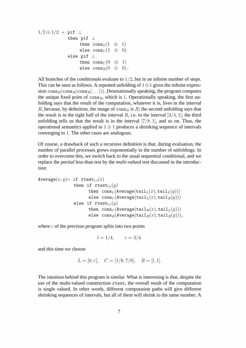
1/2 ⊕ 1/2 = pif ⊥then pif ⊥

then consL(1 ⊕ 1)else consC(1 ⊕ 0)

else pif ⊥then consC(0 ⊕ 1)else consR(0 ⊕ 0).

All branches of the conditionals evaluate to1/2, but in an infinite number of steps.This can be seen as follows. A repeated unfolding of1⊕1 gives the infinite expres-sionconsR(consR(consR(. . . ))). Denotationally speaking, the program computesthe unique fixed point ofconsR, which is1. Operationally speaking, the first un-folding says that the result of the computation, whatever itis, lives in the intervalR, because, by definition, the image ofconsR is R; the second unfolding says thatthe result is in the right half of the intervalR, i.e. in the interval[3/4, 1]; the thirdunfolding tells us that the result is in the interval[7/8, 1], and so on. Thus, theoperational semantics applied to1 ⊕ 1 produces a shrinking sequence of intervalsconverging to1. The other cases are analogous.

Of course, a drawback of such a recursive definition is that, during evaluation, thenumber of parallel processes grows exponentially in the number of unfoldings. Inorder to overcome this, we switch back to the usual sequential conditional, and wereplace thepartial less-than test by themulti-valuedtest discussed in the introduc-tion:

Average(x, y)= if rtestl,r(x)then if rtestl,r(y)

then consL(Average(tailL(x), tailL(y)))else consC(Average(tailL(x), tailR(y)))

else if rtestl,r(y)then consC(Average(tailR(x), tailL(y)))else consR(Average(tailR(x), tailR(y))),

wherec of the previous program splits into two points

l = 1/4, r = 3/4.

and this time we choose

L = [0, r], C = [1/8, 7/8], R = [l, 1].

The intuition behind this program is similar. What is interesting is that, despite theuse of the multi-valued constructionrtest, the overall result of the computationis single valued. In other words, different computation paths will give differentshrinking sequences of intervals, but all of them will shrink to the same number. A

7

proof of this fact and of correctness of the program is provided in Section 6, usingthe techniques developed below. For further examples see [22].

3 Background

For domain-theoretic concepts, the reader is referred to [1,27], and for topologicalconcepts to [33,34] (see also [16]). Here we briefly summarize the notions and factsthat are relevant to our purposes.

3.1 Continuous Domains

Let P be a set with a preorder⊑. For a subsetX of P and an elementx ∈ P wewrite

↓X = {y ∈ P | y ⊑ x for somex in X},

↑X = {y ∈ P | x ⊑ y for somex in X},

↓x = ↓{x}, ↑x = ↑{x}.

We also say thatX is a lower setiff X = ↓X, and thatX is an upper setiffX = ↑X.

Let x andy be elements of a directed complete partial order (dcpo)D. We say thatx is way-belowor approximatesy, denotedx ≪ y, if for every directed subsetA ofD, y ⊑

⊔A implies∃a ∈ A with x ⊑ a. We say thatx iscompactif it approximates

itself. We define↑↑x = {y ∈ D | x ≪ y}, ↓↓x = {y ∈ D | y ≪ x} andK(D) ={x ∈ D | x is compact}. We say that a subsetB of a dcpoD is abasisfor D, if forevery elementx of D the set↓↓x ∩ B contains a directed subset with supremumx.A dcpo is called acontinuous domainor simply a domain if it has a basis. A dcpois called analgebraic domainif it has a basis of compact elements. An exampleof an algebraic domain is the domainT⊥ = {⊥, false, true} of booleans, orderedby ⊥ ⊑ false,⊥ ⊑ true. A function f from a domainD to a domainE is Scottcontinuos if it is monotone andf(

⊔A) =

⊔f(A) for all directed subsetA of D. A

Scott closed subset of a domainD is a lower set closed under directed supremum.We say that a Scott closed set is finitely generated if it is thelower set of a finiteset. The following is easily established:

Lemma 3.1 If D is a continuous domain,C a finitely generated Scott closed subsetof D andf : D → D Scott continuous then

↓{f(x) | x ∈ C} = cl{f(x) | x ∈ C}.

wherecl denotes topological (Scott) closure.

8

3.2 The Interval DomainsR andI

The setR of non-empty compact subintervals of the Euclidean real line ordered byreverse inclusion,

x ⊑ y iff x ⊇ y,

is a continuous domain, referred to as theinterval domain. Here intervals are re-garded as “partial numbers”, with the singleton intervals playing the role of “totalnumbers”. If we add a bottom element toR, thenR becomes a bounded completecontinuous domainR⊥. For any intervalx ∈ R, we write

x = inf x andx = sup x

so thatx = [x, x]. Its length is defined by

κx = x − x.

A subsetA ⊆ R has a least upper bound iff it has non-empty intersection, and inthis case

⊔A =

⋂A =

[supa∈A

a, infa∈A

a

].

The way-below relation ofR is given by

x ≪ y iff x < y andy < x.

A basis forR is given by the intervals with distinct rational (alternatively dyadic)end-points.

The setI of all non-empty closed intervals contained in the unit interval [0, 1]is a bounded complete, countably based continuous domain, referred as theunitinterval domain. The bottom element ofI is the interval[0, 1].

3.3 Powerdomains

Powerdomains [25,31,32] are usually constructed as ideal completions [18] of finitesubsets of basis elements. For our purposes, it is more convenient to work withtheir topological representations [27,1,19], which we nowsummarize. It is enoughfor our purposes to restrict attention toω-continuous dcpos, which we refer to asdomainsin this subsection.

A subsetA of a dcpoD is calledScott closedif it is closed in the Scott topology,that is, if it is a lower set and is closed under the formation of suprema of directedsubsets. We use the notationcl(A) for the topological closure ofA, i.e. the smallest

9

Scott closed set containingA. A lenseis a non-empty set that arises as the intersec-tion of a Scott-closed set and a Scott compact upper subset. Here the notion of Scottcompact set is to be understood in the topological sense (every cover consisting ofScott open sets has a finite subcover). On the set of lenses of adcpoD, we define thetopological Egli-Milner ordering,⊑TEM by K ⊑TEM L if L ⊆ ↑K andK ⊆ cl(L).Notice that in a finite domain such as the flat domain of booleans, the lenses arejust order-convex sets, and that the topological Egli-Milner order coincides withthe usual order-theoretical one [16]. This is because in a finite domain the closedsets are precisely the lower sets, and all sets are compact.

ThePlotkin powerdomainPP D of a domainD consists of the lenses ofD underthe Egli-Milner order, and the formal-union operationA ∪ B is given by actualunion A ∪ B followed by topological convex closure (intersection of all convexclosed sets containing it). There is a natural topological embeddingη : D → PP Dgiven byx 7→ {x}.

TheSmyth powerdomainPSD consists of the set of non-empty Scott-compact up-per subsets ordered byreverseinclusion, with formal union given by actual union.In this case, we have a natural topological embeddingη : D → PSD given byx 7→ ↑x

The Hoare powerdomainPHD consists of all non-empty Scott-closed subsets ofD ordered by inclusion. Because we use this to obtain a denotational model of ourlanguage, we consider it in more detail. Least upper bounds are given by

⊔

i∈I

Ai = cl⋃

i∈I

Ai.

The construction is the functor part of a monad, with action on continuous mapsgiven by

f : PHD → PHE

A 7→ clf [A]

for anyf : D → E. Its unit is given by

ηD : D → PHD

x 7→ ↓x,

which is also a topological embedding. Instead of considering multiplication, onecan equivalently consider the extension operator [21, Proposition 2.14], in this casegiven by

f : PHD → PHE

A 7→ cl⋃

a∈A fa

for any continuous mapf : D → PHE. Finally, formal unions are given by actual

10

unions as in the case of the Smyth powerdomain:

A ∪ B = A ∪ B.

4 Semantics of the Multi-valued Construction

In order to make the development of the introduction precise, we assume that we aregiven a functorial powerdomain constructionP, in a suitable category of domains,with a natural embedding

ηD : D → PD

and a continuous formal-union operation

(− ∪ −) : PD × PD → PD

for every domainD. Then the definition of the functionrtesta,b : R → PT, wherea < b are real numbers, can be formulated as

rtesta,b(x) =

η(true), if x ∈ (−∞, a],

η(true) ∪ η(false), if x ∈ (a, b),

η(false), if x ∈ [b,∞).

Because in our language there will be computations on the reals that diverge orfail to fully specify a real number, we need to embed the real line into a domainof total and partial real numbers. We choose to work with the domainR⊥, whereR is the interval domain introduced in Section 3. Similarly, as usual, we enlargethe domainT of booleans with a bottom element. Hence we have to work with anextensionR⊥ → PT⊥ of the above function, which we denote by the same name:

Rrtesta,b−−−−→ PTy

y

R⊥rtesta,b

−−−−→ PT⊥

For the moment, we do not insist on any particular extension.However, in order fora powerdomain construction to qualify for a denotational model of the language,the minimum requirement is that it makes thertesta,b function continuous.

Lemma 4.1 If rtesta,b : R⊥ → PT⊥ is a continuous extension of the functionrtesta,b : R → PT, then the inequalities

η(true) ⊑ η(true) ∪ η(false),

η(false) ⊑ η(true) ∪ η(false)

11

must hold in the powerdomainPT⊥

PROOF. Because the embeddingR → R⊥ is continuous whenR is endowedwith its usual topology andR⊥ with its Scott topology, so is its composition withthe functionrtesta,b : R⊥ → PT⊥, which we denote byr : R → PT⊥. (This isthe diagonal of the above commutative square). In any dcpo, the relationd ⊑ eholds if and only if every neighbourhood ofd is a neighbourhood ofe. Let V be aneighbourhood oft := η(true). We have to show thatn := η(true) ∪ η(false) ∈ V .The setU := r−1(V ) is open inR by continuity ofr : R → PT. Becauser(a) =t ∈ V , we have thata ∈ r−1(V ) = U . Hence, becauseU is open inR, there isan open interval(u, v) with a ∈ (u, v) ⊆ U . Choosex such thata < x < v andx < b, that is, such thatx ∈ (a, b) ∩ (u, v) ⊆ U . By construction,r(x) = n. Butx ∈ r−1(V ), which shows thatn ∈ V and hence thatt ⊑ n, which amounts to thefirst inequality. The second inequality is obtained in the same way. 2

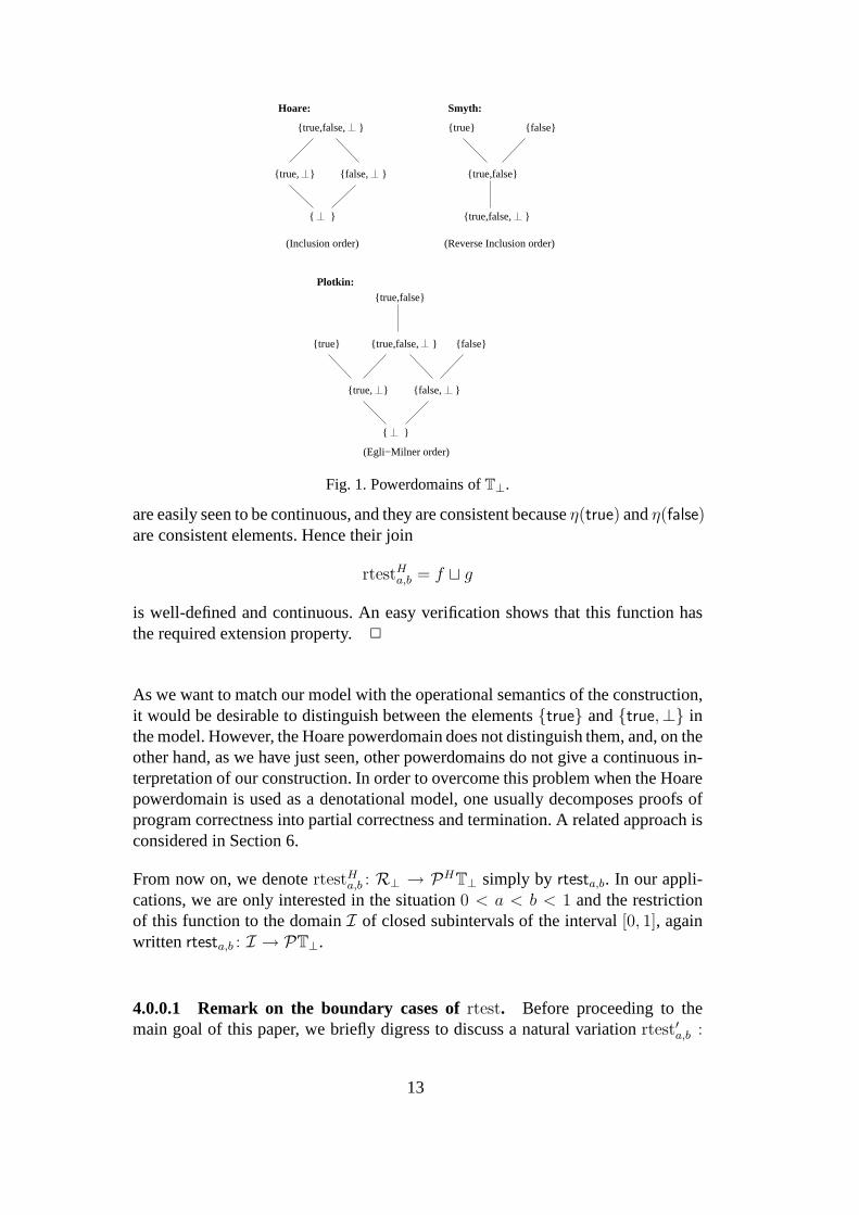
Thus, any powerdomain not satisfying the above two inequalities does not qualifyfor a model. In particular, this rules out the Plotkin and Smyth powerdomains. Infact, for the Plotkin powerdomain one has thatη(true) = {true} andη(false) ={false}, and their formal union is{true, false} because this set is order-convex,but the sets{true} and {true, false} are incomparable in the Egli-Milner order.For the Smyth powerdomain, the same sets are obtained by the embedding, formalunion is given by actual union, and hence the inequalities donot hold because theorder is given by reverse inclusion. We omit routine proofs of the fact that e.g. themixed [17] and the sandwich [5] powerdomains also fail to satisfy the inequalitiesand hence to make thertesta,b construction continuous.

On the other hand, for the Hoare powerdomain, the inequalities do hold. In fact,η(true) = {true,⊥} andη(false) = {false,⊥}, their formal union is their actualunion{true, false,⊥}, and the ordering is given by inclusion. Moreover:

Proposition 1 There is a continuous extensionrtestHa,b : R⊥ → PHT⊥ of the func-

tion rtesta,b : R → PT.

PROOF. The functionsf, g : R⊥ → PT⊥ defined by

f(x) =

η(true), if x ⊆ (−∞, b),

⊥, otherwise,

g(x) =

η(false), if x ⊆ (a,∞),

⊥, otherwise,

12

{true,false, }

{true, } {false, }

{ }

{true,false, }

{true, } {false, }

{ }

{false}

{true,false}

{true}

Smyth:

(Reverse Inclusion order)

{true,false, }

(Egli−Milner order)

{true,false}

{true} {false}

(Inclusion order)

Plotkin:

Hoare:

Fig. 1. Powerdomains ofT⊥.

are easily seen to be continuous, and they are consistent becauseη(true) andη(false)are consistent elements. Hence their join

rtestHa,b = f ⊔ g

is well-defined and continuous. An easy verification shows that this function hasthe required extension property.2

As we want to match our model with the operational semantics of the construction,it would be desirable to distinguish between the elements{true} and{true,⊥} inthe model. However, the Hoare powerdomain does not distinguish them, and, on theother hand, as we have just seen, other powerdomains do not give a continuous in-terpretation of our construction. In order to overcome thisproblem when the Hoarepowerdomain is used as a denotational model, one usually decomposes proofs ofprogram correctness into partial correctness and termination. A related approach isconsidered in Section 6.

From now on, we denotertestHa,b : R⊥ → PHT⊥ simply by rtesta,b. In our appli-

cations, we are only interested in the situation0 < a < b < 1 and the restrictionof this function to the domainI of closed subintervals of the interval[0, 1], againwritten rtesta,b : I → PT⊥.

4.0.0.1 Remark on the boundary cases ofrtest. Before proceeding to themain goal of this paper, we briefly digress to discuss a natural variation rtest′a,b :

13

R → PT of thertesta,b construction, defined by

rtest′a,b(x) =

η(true), if x ∈ (−∞, a),

η(true) ∪ η(false), if x ∈ [a, b],

η(false), if x ∈ (b,∞).

With a proof similar to that of Lemma 4.1, we conclude that ifrtest′a,b is continuousthen

η(true) ∪ η(false) ⊑ η(true)

η(true) ∪ η(false) ⊑ η(false).

This rules out the Plotkin and Hoare powerdomains, but not the Smyth powerdo-main. However, it is not clear what the operational counterpart of this functionwould be. The functionrtesta,b is operationally computable because, for any argu-mentx given intensionally as a shrinking sequence of intervals, the computationalrules systematically establish one of the semidecidable conditionsa < x andx < b.However, the conditionsa ≤ x andx ≤ b are not semi-decidable, and hence it isnot immediately apparent what a computationally adequate operational semanticsfor rtest′ would be. But it is interesting, as pointed out by one of the referees, thatthe cotransitivity law given in the introduction as a constructive justification ofrtestcan be equivalently formulated as “a ≤ x or x ≤ b whenevera < b”. In any case,it is not clear to us, at the time of writing, whether or how this reformulation of thecotransitivity law would lead to a computational mechanismfor rtest′.

5 A Programming Language for Sequential Real-Number Computation

We introduce the language LRT for thertest construction, which amounts to thelanguage considered by Escardo [11] with the parallel conditional removed and aconstant forrtesta,b added. We remark that this is a call-by-name language. Becausereal-number computations are infinite, and there are no canonical forms for partialreal-number computations, it is not clear what a call-by-value operational semanticsought to be. We leave this as an open problem.

5.1 Syntax

The language LRT is an extension of PCF with a ground type for real numbers andsuitable primitive functions for real-number computation. Its raw syntax is givenby

14

x ∈ V ariable,

t ::= nat | bool | I | t → t,

P ::= x | n | true | false | (+1)(P ) | (−1)(P ) |

(= 0)(P ) | ifP thenP elseP | consa(P ) |

taila(P ) | rtesta,b(P ) | λx : t.P | PP | YP,

where the subscripts of the constructscons, tail are rational intervals and thoseof rtest are rational numbers. (We apologize for using the lettersa andb to denotenumbers and intervals in different contexts.) Terms of ground typeI are intendedto compute real numbers in the unit interval.

It is convenient for our purposes to first define the denotational and then the opera-tional semantics.

5.2 Denotational Semantics.

The ground typesbool, nat andI are interpreted as the Hoare powerdomain of thedomains of booleans, natural numbers and intervals, respectively. Function typesare interpreted as function spaces in the category of dcpos:

JboolK = PHT⊥, JnatK = PHN⊥, JIK = PHI,

Jσ → τK = JσK → JτK.

This reflects the fact that we are considering a call-by-namelanguage.

The interpretation of constants in LRT is defined as follows:

JtrueK = η(true), JfalseK = η(false), JnK = η(n),

J(+1)K = (+1), J(−1)K = (−1), J(= 0)K = (= 0),

JconsaK = consa, JtailaK = taila,

Jrtesta,bK = rtesta,b, JYK(F ) =⊔

n≥0

F n(⊥),

JifK(B, X, Y ) =

X, if B = η(true),

Y, if B = η(false),

X ∪ Y, if B = η(true) ∪ η(false),

⊥, if B = ⊥.

Here the symbolsη, , are defined as in Section 3.3, the functions(+1), (−1), (= 0)are the standard interpretations in the Scott model of PCF, the functionsconsa, tailaare defined in Section 2, and the functionrtesta,b is defined in Section 4.

15

5.3 Operational Semantics

We consider a small-step style operational semantics for our language. We definethe one-step reduction relation→ to be the least relation containing the one-stepreduction rules for evaluation of PCF [26] together with those given below.

We first need some preliminaries. For intervalsa andb in I, we define

ab = consa(b),

wherecons is the extension to the interval domain of the function defined in Sec-tion 2. This operation is associative, and has the bottom element ofI as its neutralelement [11]:

(ab)c = a(bc), a⊥ = ⊥a = a.

Moreover,

a ⊑ b ⇐⇒ ∃c ∈ I. ac = b,

and thisc is unique ifa has non-zero length, i.e. it is not maximal, and in this casewe denotec by

b \ a.

For intervalsa andb, we define

a ≤ b ⇐⇒ a ≤ b

and

a ↑ b ⇐⇒ ∃c. a ⊑ c andb ⊑ c.

With this notation, the rules for Real PCF as defined in [11] are:

16

(1) consa(consbM) → consabM

(2) consaM → consaM′ if M → M ′ & (1) is not

applicable

(3) taila(consbM) → YconsL if b ≤ a

(4) taila(consbM) → YconsR if b ≥ a

(5) taila(consbM) → consb\aM if a ⊑ b anda 6= b

(6) taila(consbM) → cons(a⊔b)\a(tail(a⊔b)\bM) if a ↑ b, a 6⊑ b, b 6⊑ a,b � a anda � b

(7) taila(M) → taila(M′) if M → M ′ & (3)-(6) are

not applicable

(8) if true M N → M

(9) if false M N → N

(10) if M N1 N2 → if M ′ N1 N2 if M → M ′ & (8),(9) arenot applicable

For our languageLRT , we add:

(11) rtestb,c(consa M) → true if a < c,(12) rtestb,c(consa M) → false if b < a,(13) rtestb,c M → rtestb,c M

′

if M → M′

.

Remark 5.1

(1) Rule 1 plays a crucial role and amounts to the associativity law. The idea isthat botha andb give partial information about a real number, andab is theresult of gluing the partial information together in an incremental way. See thepaper [11] for a further discussion, including a geometrical interpretation.

(2) Notice that if the intervala is contained in the interval[b, c], rules 11 and 12can be applied.

(3) Rules 11-13 cannot be made deterministic given the particular computationaladequacy formulation which is proved in Section 5.4. We shall show that theset of rewrite rules is rich enough to allow one to derive operationally every-thing that the denotational semantics suggests. This does not mean that weare giving a specification for an implementation ofLRT . In the absense ofrtestb,c, the rules 1-10 are deterministic without loss of computational ade-quacy. See Section 6 for a further discussion.

(4) In practice, one would like to avoid divergent computations by consideringa strategy for application of the rules. This is the topic of Section 6 wherewe study total correctness. For the purposes of this section, we consider thenon-deterministic view.

We now introduce a notion of operational meaning of a term, where the operational

17

values are taken in a powerdomain too. The difference between this operationalsemantics and the denotational semantics given above is that the former is obtainedby reduction but the latter is obtained, as usual, by compositional means.

Definition 5.2 Firstly, we define the operational meaning of closed termsM ofground typesγ in i steps of computation, written[M ]i, which is to be an element ofthe domainJγK.

If M : I, then we define

[M ]i = ∪ {η(a) | ∃M ′∃k ≤ i, Mk→ consaM

′}.

(If this set is empty, then of course[M ]i = ⊥.) Here the relation k→ denotes the

k-fold composition of the relation→.

If M : nat, then we define

[M ]i = ∪ {η(n) | ∃k ≤ i, Mk→ n}

if this set is non-empty, and[M ]i = ⊥ otherwise. The operational meaning ofM : bool is defined similarly.

It is immediate that[M ]i ⊑ [M ]i+1. Hence we can define

[M ] =⊔

i

[M ]i.

Of course, only in the case of the ground type of real numbers this definition isnon-trivial, but it is convenient to have a uniform treatment for all types.

5.4 Computational Adequacy.

In our setting,computational adequacyamounts to the equation[M ] = JMK for allclosed termsM of ground type, where[M ] is the operational meaning ofM andJMK is the denotational meaning ofM defined above.

For a deterministic language such as PCF, soundness of the denotational semanticsfollows from the fact thatM → N impliesJMK = JNK. For our non-deterministiclanguage, we rely on the following:

Lemma 5.3 JMK =∪ {JNK | M → N} (notice that this is a finite union).

PROOF. The proof is by structural induction onM .

If M is a value, there is nothing to prove.

18

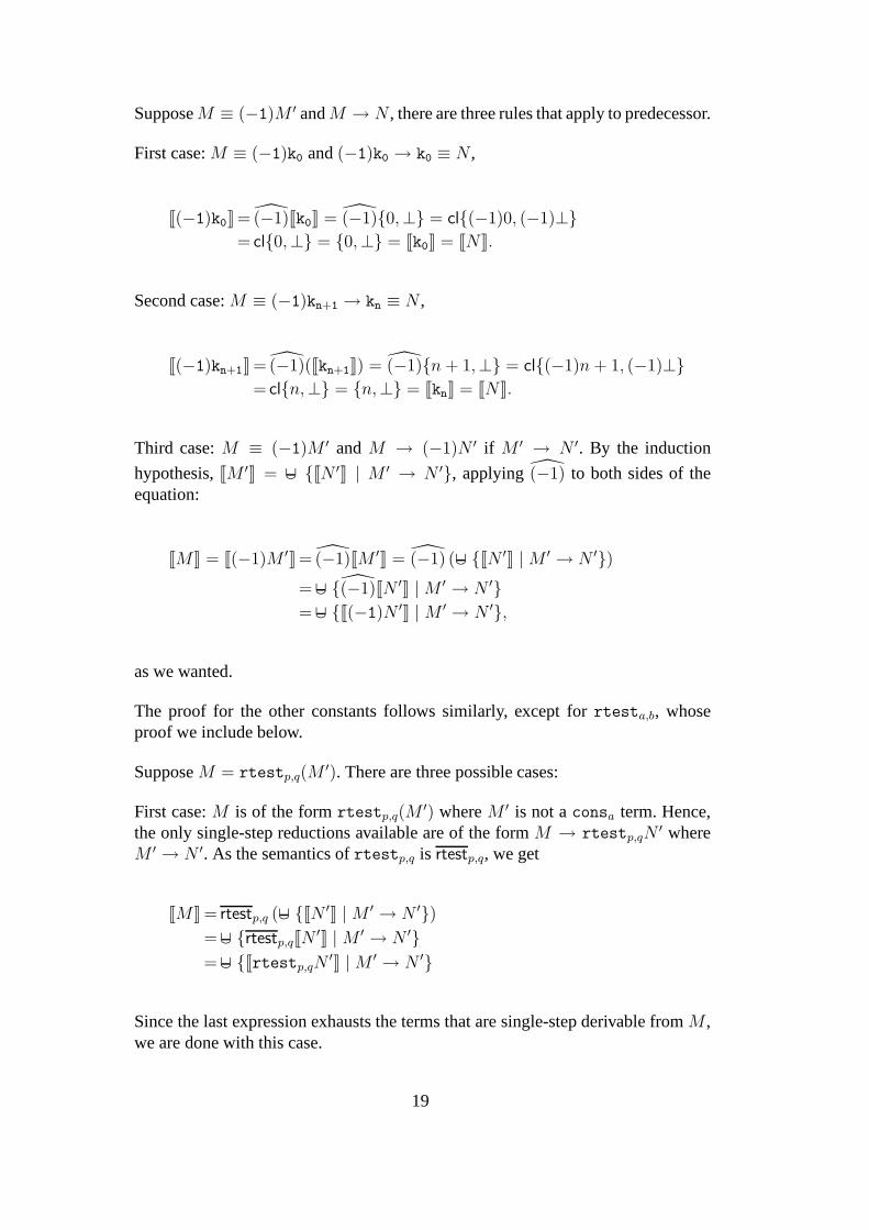
SupposeM ≡ (−1)M ′ andM → N , there are three rules that apply to predecessor.

First case:M ≡ (−1)k0 and(−1)k0 → k0 ≡ N ,

J(−1)k0K= (−1)Jk0K = (−1){0,⊥} = cl{(−1)0, (−1)⊥}

= cl{0,⊥} = {0,⊥} = Jk0K = JNK.

Second case:M ≡ (−1)kn+1 → kn ≡ N ,

J(−1)kn+1K = (−1)(Jkn+1K) = (−1){n + 1,⊥} = cl{(−1)n + 1, (−1)⊥}

= cl{n,⊥} = {n,⊥} = JknK = JNK.

Third case:M ≡ (−1)M ′ and M → (−1)N ′ if M ′ → N ′. By the induction

hypothesis,JM ′K = ∪ {JN ′K | M ′ → N ′}, applying (−1) to both sides of theequation:

JMK = J(−1)M ′K= (−1)JM ′K = (−1) (∪ {JN ′K | M ′ → N ′})

=∪ {(−1)JN ′K | M ′ → N ′}

=∪ {J(−1)N ′K | M ′ → N ′},

as we wanted.

The proof for the other constants follows similarly, exceptfor rtesta,b, whoseproof we include below.

SupposeM = rtestp,q(M′). There are three possible cases:

First case:M is of the formrtestp,q(M′) whereM ′ is not aconsa term. Hence,

the only single-step reductions available are of the formM → rtestp,qN′ where

M ′ → N ′. As the semantics ofrtestp,q is rtestp,q, we get

JMK = rtestp,q (∪ {JN ′K | M ′ → N ′})

=∪ {rtestp,qJN′K | M ′ → N ′}

=∪ {Jrtestp,qN′K | M ′ → N ′}

Since the last expression exhausts the terms that are single-step derivable fromM ,we are done with this case.

19

Second case:M is of the formrtestp,q(consa(M′′)). Note that the above equality

still holds but the last∪ does not exhaust the single-step derivations. Furthermore,

JMK = rtestp,q(consa(M′)) ⊒ rtestp,q(a).

As ∪ is inflationary, we can throw smaller terms into the above equation:

JMK =∪ {rtestp,qN′ | M ′ → N ′}

= rtestp,q(a) ∪(⋃

{Jrtestp,qN′K | M ′ → N ′}

)

Now rtestp,q(a) is exactly the set⋃

{JbK | M → b andb ∈ {true, false}} . 2

Hence, by induction on the lengthj of the evaluation using the previous lemma, for

everyj, JMK = ∪ {JNK | Mj→ N}.

Lemma 5.4 (Soundness)For all closed terms M of ground type,

[M ] ⊑ JMK.

PROOF. It suffices to show that, for all closed termsM of ground type,

[M ]i ⊑ JMK.

Let b ∈ [M ]i, b 6= ⊥. By definition,b ⊑ a for somea andM ′ such thatM i→

consaM′. BecauseconsaJM

′K = JconsaM′K, Lemma 5.3 shows thatb ∈ ↓JconsaM

′K.Thereforeb ∈ JMK becausea ⊑ consa(x) for all x ∈ I, and in particular for allx ∈ JM ′K. 2

In order to establish completeness, we proceed as in [26,11].

Definition 5.5 We define a notion of computability for closed terms by inductionon types as follows:

(1) A closed termM of ground type is computable wheneverJMK ⊑ [M ],(2) A closed termM : σ → τ is computable wheneverMQ : τ is computable for

every closed computable termQ of typeσ,

An open termM : σ with free variablesx1, . . . , xn of typeσ1, . . . , σn is computablewhenever[N1/x1] · · · [Nn/xn]M is computable for every familyNi : σi of closedcomputable terms.

20

BecausePH(D) is a continuous domain ifD is, we have:

Lemma 5.6 A closed termM of ground type is computable iff for everyX ≪ JMKthere isi with X ⊑ [M ]i.

PROOF. (⇒) Suppose thatM is computable and letX ≪ JMK. We have that[M ]1 ⊑ [M ]2 ⊑ · · · is a chain whose supremum is[M ], and hence there isi withX ⊑ [M ]i. (⇐) By continuity of the Hoare powerdomain of a continuous domain,in order to show thatJMK ⊑ [M ], it suffices to show that for allX ≪ JMK,X ⊑ [M ]. But this holds by hypothesis.2

Recall the following from domain theory [1,16].

Lemma 5.7 For any continuous functionf : D → E of continuous dcpos, ify ≪f(x) then there isx′ ≪ x with y ≪ f(x′).

Lemma 5.8 (Completeness)Every term is computable.

PROOF. The proof is by structural induction on the formation rules of terms.

Constants:(1) rtestp,q is computable:

We have to show thatJrtestp,qMK ⊑ [rtestp,qM ]

for computableM . So

Jrtestp,qMK = rtestp,qJMK

⊑ rtestp,q[M ]

= rtestp,q

⊔

i

[M ]i

=⊔

i

rtestp,q[M ]i

=⊔

i

rtestp,q

⋃ {η(a) | ∃M ′∃k ≤ i.M →k consaM

′}

=⊔

i

⋃ {rtestp,q(η(a)) | ∃M ′∃k ≤ i.M →k consaM

′}

=⊔

i

⋃ {rtestp,q(a) | ∃M ′∃k ≤ i.M →k consaM

′}

.

But whenM →k consaM′ holds, so doesrtestp,q(a) ⊑ [rtestp,qM ]k+1 ⊑

[rtestp,qM ]. So the directed sup of formal joins also lies below[rtestp,qM ].

21

(2) if is computable:

We have to show that

Jif L M NK ⊑ [if L M N ].

Supposeη(true) ⊑ JLK. By the induction hypothesis,JLK ⊑ [L], soL →l true

for somel. Thusif L M N →l+1 M . Hence,JMK ⊑ [if L M N ]. Similarly,if η(false) ⊑ JLK, thenJMK ⊑ [if L M N ]. Now, we need the four cases ofthe proof: if JLK = η(⊥), thenJif L M NK = η(⊥); if JLK = η(true), thenJif L M NK = JMK; if JLK = η(false), thenJif L M NK = JNK; and if JLK =η(true) ∪ η(false), thenJif L M NK = JMK ∪ JNK. Because∪ is inflationary(andη(⊥) is the identity for it); in all four casesJif L M NK ⊑ [if L M N ].

(3) consa is computable:

We have to show that ifM is computable, then so isconsaM .

Assume thatJconsaMK 6= ⊥ for a computable termM of type I. Let Y ≪JconsaMK = consaJMK. We need to show that there isi with Y ⊑ [consaM ]i. ByLemma 5.7, there isX ≪ JMK with Y ≪ consaX. As M is computable, there isjsuch thatX ⊑ [M ]j . BecauseY ⊑ consaX and by monotonicity ofconsa, we havethatY ⊑ consa[M ]j . So for everyy ∈ Y , there ism ∈ consa[M ]j , with y ⊑ m.Let m ∈ consa[M ]j , by Lemma 3.1 there ist ∈ [M ]j with m ⊑ consa(t) = at.Because there ist ∈ [M ]j , we deduce that there isM ′ such that the reduction

Mk→ constM

′, k ≤ j holds, and soconsaMk→ consa(constM

′)1→ consatM

′.Hence we can takei = j + 1.

(4) taila is computable:

We have to show that ifM is computable, then so istailaM . Assume thatJtailaMK 6= ⊥ for a computable termM of type I. Let Y ≪ JtailaMK =

tailaJMK. We need to show that there isi with Y ⊑ [tailaM ]i. By lemma 5.7,there isX ≪ JMK with Y ≪ tailaX. As M is computable, there isj such thatX ⊑ [M ]j . BecauseY 6= {⊥}, it follows that [M ]j 6⊑ {a} in the Egli–Milner or-der, and if[M ]j ⊑ {a} thenY ≪ tailaX ⊑ taila[M ]j ⊑ taila{a} = cl{⊥} = {⊥}.Then exactly one of the following four cases holds:

(a) [M ]j ≤ {a}: Then sinceX ⊑ [M ]j , we have thattailaX ⊑ taila[M ]j and sinceY ⊑ tailaX, we haveY ⊑ taila[M ]j . So for everyy ∈ Y , there ism ∈ taila[M ]jwith y ⊑ m. Letm ∈ taila[M ]j , so by lemma 3.1 there ist ∈ [M ]j with m ⊑ tailat.

Because there ist ∈ [M ]j it follows that there isM ′ such thatM k→ constM

′, k ≤

j holds. Because[M ]j ≤ {a} we conclude thattailaMk→ taila(constM

′)1→

YconsL. Hence we can takei = k + 1.

(b) {a} ≤ [M ]j Similar to 1.

22

(c) {a} ⊑ [M ]j : Then sinceX ⊑ [M ]j , we have thattailaX ⊑ taila[M ]j = {b \ a |

b ∈ [M ]j} and sinceY ⊑ tailaX, we have thatY ⊑ taila[M ]j . So for everyy ∈ Y ,there ism ∈ taila[M ]j with y ⊑ m. Let m ∈ taila[M ]j , so there ist ∈ [M ]j withm ⊑ tailat = t \ a. Because there ist ∈ [M ]j it follows that there isM ′ such that

Mk→ constM

′, k ≤ j holds. We conclude thattailaMk→ taila(constM

′)1→

tailmM ′. Hence we can takei = k + 1.

(d) {a} ↑ [M ]j : Then sinceX ⊑ [M ]j , we have thattailaX ⊑ taila[M ]j = {(a ⊔

b) \ a | b ∈ [M ]j} and sinceY ⊑ tailaX, we have thatY ⊑ taila[M ]j . So foreveryy ∈ Y , there ism ∈ taila[M ]j with y ⊑ m. Let m ∈ taila[M ]j , so there ist ∈ [M ]j with m ⊑ tailat = (a ⊔ t) \ a. Because there ist ∈ [M ]j it follows that

there isM ′ such that the reductionM k→ constM

′, k ≤ j holds. We conclude thattailaM

k→ taila(constM

′)1→ tailmM ′. Hence we can takei = k + 1.

(5) ForM ≡ (+1), (−1), (= 0) the proof is similar to theif case.

(6) If M is computable so isλαM :

We must show thatLN1, . . .Nn is computable wheneverN1, . . . Nn are closed com-putable terms andL is a closed instantiation ofλαM by computable terms. HereLmust have the formλαM ′ whereM ′ is an instantiation of all free variables ofM ,exceptα, by closed computable terms.

If P ≪ JLN1 . . . NnK then we haveP ≪ J[N1/α]M ′N2 . . . NnK = JLN1 . . . NnK.But [N1/α]M ′ is computable and so therefore[N1/α]M ′N2 . . . Nn. Hence thereis j with P ⊑ [[N1/α]M ′N2 . . . Nn]j . SinceLN1 . . . Nn → [N1/α]M ′N2 . . . Nn

and the reduction relation preserves meanings, in order to evaluateLN1 . . . Nn itsuffices to evaluate[N1/α]M ′N2 . . . Nn. Hence we can takei = j.

(7) Yσ is computable:

In order to prove thatYσ is computable it suffices to show that the term

Y(σ1,...,σk,PI)N1 · · ·Nk

is computable wheneverN1 : σ1, . . . , Nk : σk are closed computable terms. It fol-lows from (6) above that the termsY(n)

σ := λf.fn(⊥) are computable, becausethe proof of computability ofY(n)

σ depends only on the fact that variables are com-putable and that the combination and abstraction formationrules preserve com-putability.

Let P ≪ JYN1 · · ·NKK be different from⊥. BecauseJYK =⊔

JY(n)K, by a ba-sic property of the way-below relation of any continuous dcpo, there is somensuch thatP ≪ JY(n)N1 · · ·NKK. SinceY(n) is computable, there isj with P ⊑

[Y(n)N1 · · ·Nk]j. Since there is a termM with Y(n)N1 · · ·Nkj→ conscM . Using

23

thesyntactic information order(see [26,11]), and Lemma 5.9 below,Y(n) 4 Y we

have thatYN1 · · ·Nkj→ conscM for someM and thereforei = j. 2

As in the last part of the above proof, we denote the syntacticorder by4 (see [26]or [11]).

Lemma 5.9 If M 4 N and M → M1, M → M2, · · · , M → Mn then either∀i, Mi 4 N, 1 ≤ i ≤ n or else for some termsN1, N2, . . . , Nm, N → N1, N →N2, · · · , N → Nm, and∀Mi, ∃Nj , Mi 4 Nj, 1 ≤ i ≤ n, 1 ≤ j ≤ m

PROOF. The case that we must consider is the one that involvesrtesta,b. Theother cases are treated as in Real PCF.

(1) rtesta,bM 4 rtesta,bM holds by definition.

(2) M ≡ rtesta,bM′ 4 rtesta,bM

′′ ≡ N andM → true. These conditionshold if rtesta,bM → rtesta,b(conscM

′′′) and c < b. By the induction hy-pothesis,M ′ → M ′′ so rtesta,bM

′′ → rtesta,b(consdMiv) whered < b so

rtesta,bM′′ → true andtrue 4 true.

(3) M ≡ rtesta,bM′ 4 rtesta,bM

′′ ≡ N and M → false. Similar to theprevious case.

(4) M ≡ rtesta,bM′ 4 rtesta,bM

′′ ≡ N andM → true, M → false. Thesefollows if rtesta,bM → rtesta,b(conscM

′′′) anda < c < b. By the inductionhypothesis,M ′ → M ′′ so rtesta,bM

′′ → rtesta,b(consdMiv) wherea < d <

b so rtesta,bM′′ → true, rtesta,bM

′′ → false and true 4 true, false 4

false. 2

In summary:

Theorem 5.10 Computational adequacy holds; that is, for every closed termM ofground type, the operational and denotational meanings ofM coincide:

[M ] = JMK.

6 Program Correctness

We now develop tools for establishing correctness ofLRT programs. In order toshow that a given program is correct with respect to a given specification, we showthat

24

(1) if it converges, then it satisfies the specification, and(2) it in fact converges.

In our examples, condition 1 will be achieved by applying thedenotational seman-tics with the aid of computational adequacy, and condition 2will be achieved usingthe operational semantics directly. Hence our first task is to define a suitable oper-ational notion of convergence for terms of real-number type.

Firstly, notice that the operational semantics defined in Section 5.3 allows diver-gence when rule 13 forrtesta,b is applied infinitely often. But the only purpose ofthis rule is to get a sufficiently precise approximation of the argument, so that rules11 and/or 12 can be eventually applied, provided such an approximation exists.Hence we agree that

we do not apply rule 13 forrtesta,b infinitely often unless rules 11-12 are neverapplicable.

Definition 6.1 The subrelation of the reduction relation→ that arises in this waywill be denoted by⇒.

Secondly, in the case of a term of the formrtesta,b(M), after finitely many appli-cations of rule 13 to compute an approximation of the argument M , we will havethree situations:

(1) Both rules 11 and 12 become applicable.(2) One and only one of the rules 11 and 12 becomes applicable.(3) It is still not possible to apply rules 11 and 12, and henceone should keep

applying rule 13, getting better and better approximationsof M , either(a) for ever, or(b) so that we eventually arrive at one of the previous situations (1) or (2),

and the computation converges to a truth value.

If the situation (3a) may take place, we say that the termmay diverge, and other-wise, that itmust converge. If the situation (1) takes place, we may imagine thatthe computation bifurcates into two subcomputations, eachof which will give ananswer or diverge. For our definition of strong convergence,to be given below,we require that both converge. In practice, an implementation of the language willtypically choose one of the branches, according to some strategy, which will notnecessarily be known to the programmer, and such a branch will then lead to ananswer or divergence. In this case, the programmer has to ensure that any possibleanswer satisfies the desired specification, or that both branches will in fact lead tothe same answer (as will be the case with our running example).

In theory, if situation (2) takes place, one can carry on withthe computation pro-duced by the corresponding branch, and, at the same time, repeatedly apply rule 13in parallel so that maybe the other rule becomes applicable too and one has two

25

computations as in situation (1). This corresponds to the relation⇒ defined above.

In practice, we work with a deterministic, but unspecified strategy, as follows:

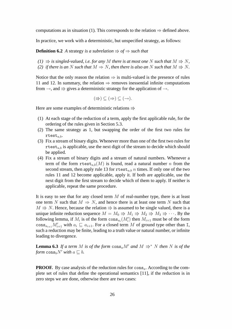
Definition 6.2 A strategyis a subrelation⇛ of ⇒ such that

(1) ⇛ is singled-valued, i.e. for anyM there is at most oneN such thatM ⇛ N ,(2) if there is anN such thatM ⇒ N , then there is also anN such thatM ⇛ N .

Notice that the only reason the relation⇒ is multi-valued is the presence of rules11 and 12. In summary, the relation⇒ removes inessential infinite computationsfrom →, and⇛ gives a deterministic strategy for the application of→.

(⇛) ⊆ (⇒) ⊆ (→).

Here are some examples of deterministic relations⇛

(1) At each stage of the reduction of a term, apply the first applicable rule, for theordering of the rules given in Section 5.3.

(2) The same strategy as 1, but swapping the order of the first two rules forrtesta,b.

(3) Fix a stream of binary digits. Whenever more than one of the first two rules forrtesta,b is applicable, use the next digit of the stream to decide which shouldbe applied.

(4) Fix a stream of binary digits and a stream of natural numbers. Whenever aterm of the formrtesta,b(M) is found, read a natural numbern from thesecond stream, then apply rule 13 forrtesta,b n times. If only one of the tworules 11 and 12 become applicable, apply it. If both are applicable, use thenext digit from the first stream to decide which of them to apply. If neither isapplicable, repeat the same procedure.

It is easy to see that for any closed termM of real-number type, there is at leastone termN such thatM ⇒ N , and hence there is at least one termN such thatM ⇛ N . Hence, because the relation⇛ is assumed to be single valued, there is aunique infinite reduction sequenceM = M0 ⇛ M1 ⇛ M2 ⇛ M3 ⇛ · · · . By thefollowing lemma, ifMi is of the formconsai

(M ′i) thenMi+1 must be of the form

consai+1M ′

i+1 with ai ⊑ ai+1. For a closed termM of ground type other thanI,such a reduction may be finite, leading to a truth value or natural number, or infiniteleading to divergence.

Lemma 6.3 If a termM is of the formconsaM′ andM ⇛∗ N thenN is of the

formconsbN′ with a ⊑ b.

PROOF. By case analysis of the reduction rules forconsa. According to the com-plete set of rules that define the operational semantics [11], if the reduction is inzero steps we are done, otherwise there are two cases:

26

(1): If consa(consbN′) ⇛ consabN

′, thenM ′ is of the formconsbN′ with a ⊑ ab.

HenceN is of the formconsabN′,

(2): If consaM′ ⇛ consaM

′′ and M ′ ⇛ M ′′, thenN has to be of the formconsaM

′′ for M ′ ⇛ N ′, and hence we can takeb = a. 2

We modify the definition of operational meaning (Definition 5.2) as follows.

Definition 6.4 For a strategy⇛ and closed termM of typeI, we define

[M ]⇛ =⊔{a ∈ I | ∃M ′.M ⇛

∗ consaM′}.

If this set is non-empty, then Lemma 6.3 shows that it is an increasing chain, andhence the supremum exists. Notice that this is not a subset ofI, as in Definition 5.2,but rather an element ofI.

By a value of typeBool or Nat we mean a constant for a truth value or a naturalnumber, and values are ranged over by the letterv. For a closed term of any ofthese two types, we define

[M ]⇛ =⊔{v | M ⇛

∗ v}.

The set of which the supremum is taken is either empty or a singleton because⇛ issingle valued.

Definition 6.5 We definestrong convergence, for closed terms, by induction ontypes as follows:

(1) A closed termM of ground type is strongly convergent if for every strategy⇛

as in Definition 6.2, its operational meaning[M ]⇛ is total (i.e. a singletoninterval, a truth-value, or a natural number).

(2) A closed termM of typeσ → τ is strongly convergent wheneverMN isstrongly convergent for every strongly convergent closed termN of typeσ.

We henceforth refer to strong convergence simply as convergence for the sake ofbrevity.

The following observation is immediate.

Lemma 6.6

(1) A termM : I is convergent iff for every strategy⇛ and everyǫ > 0 there arean intervala of length smaller thanǫ and a termN such thatM ⇛∗ consaN .

(2) A termM is convergent iffN is convergent wheneverM ⇛∗ N .

Lemma 6.7 A termconsc(M) is convergent iffM is convergent.

27

PROOF. (⇒) Let M = M1 ⇛ M2 ⇛ M3 ⇛ · · · be an infinite reduction se-quence and letǫ > 0. We must findn such thatMn is of the formconsdN

′ withκd < ǫ. Consider the reduction

consc(M) = N1 ⇛ N2 ⇛ N3 ⇛ · · · ,

andδ = ǫ× κc. By hypothesisconsc(M) is convergent so there isi such thatNi isof the formconsbN

′′ with κb < δ. Hence there should bej such thatMj is of theform conseN

′′′ andconsc(Mj) ⇛ consbN′′, which means thatκcκe = κb < δ and

henceκe < δκc

= ǫ×κc

κc= ǫ.

(⇐) Let consc(M) = N1 ⇛ N2 ⇛ N3 ⇛ · · · be an infinite reduction sequenceand letǫ > 0. We must findn such thatNn is of the formconsdN

′ with κd < ǫ.Consider the reductionM = M1 ⇛ M2 ⇛ M3 ⇛ · · · andδ = ǫ/κa. BecauseMis convergent, there isi such thatMi is of the formconsb(M

′) with κb < δ. Hence,there should bej such thatNj is of the formconse(M

′′) with κe ≤ κaκb and

κe ≤ κaκb < κa · δ = κa · (ǫ/κa) = ǫ. 2

To show thattaila is convergent, we need some lemmas. Whenever we talk aboutrules in the following lemmas, we assume that these rules aretaken from the oper-ational semantics.

Lemma 6.8

(1) For all a, b ∈ I, if b 6⊑ a then one of the conditions in rules 3–6 holds.(2) For anya ∈ I and any convergentM : I there areb 6⊑ a and N such that

M ⇛∗ consb(N).

PROOF. The first item is easily verified. For the second, letǫ = κa/2. BecauseMis convergent, there areb of length smaller thanǫ andN such thatM ⇛∗ consb(N).If we hadb ⊑ a, then the length ofb would be bigger than that ofa, which is notthe case by construction.2

Lemma 6.9 If M is convergent then,

(1) taila(M) ⇛∗ L for some convergent termL, by finitely many applicationsof rule 7 followed by an application of one of the rules 3–5, or

(2) M ⇛∗ consb(N) andtaila(M) ⇛∗ cons(a⊔b)\a(tail(a⊔b)\b(N)) for someconvergent termN , by finitely many applications of rule 7 followed by anapplication of rule 6.

28

PROOF. By Lemma 6.8, after finitely many applications of rule 7 to thetermtaila(M), we will have reductionsM ⇛∗ consb(N) and

tailaM ⇛∗ taila(consb(N)),

and one of the rules 3–6 will apply to the resulting term. If one of the rules 3–5applies thentaila(M) reduces to one of the termsYconsL, YconsR, consb\a(N),which are convergent, and we can letL be the corresponding term. Otherwise itreduces by rule 6 to the termcons(a⊔b)\a(tail(a⊔b)\b(N)). BecauseM ⇛∗ consbNandM is convergent, so areconsbN andN . 2

Lemma 6.10 The termtaila is convergent.

PROOF. Let M be convergent, consider the reduction

taila(M) = N0 ⇛ N1 ⇛ N2 ⇛ · · · ,

and let ri be the label of the rule that justifies the reductionNi ⇛ Ni+1. ByLemma 6.9, if there isi such thatri is one of 3–5, thentaila(M) is convergent,and otherwise the sequence(ri)i belongs to the set of words7∗6(7∗61)ω. We have toargue that in the second casetaila(M) is also convergent. Letni be the sequencesuch that the sequenceri can be written as7n0 6

∏i(7

ni+161).

By hypothesis, the termM0 = M is convergent, and ifMi is convergent then

Mi ⇛∗ consci

(Mi+1)

for a unique intervalci and a unique termMi+1 by finitely many applications ofrule 2, andMi+1 must also be convergent. This inductively defines sequencesci

andMi, and it is easy to see that, for anyi,

M ⇛∗ consc0c1...ci

(Mi+1).

Now, using the sequenceci, inductively define

β0 = (a ⊔ c0) \ c0, α0 = (a ⊔ c0) \ a,

βi+1 = (βi ⊔ ci+1) \ ci+1, αi+1 = (βi ⊔ ci+1) \ βi.

A routine argument by induction oni shows that

taila(M) ⇛∗ consα0α1···αi

(tailβi(Mi+1)),

29

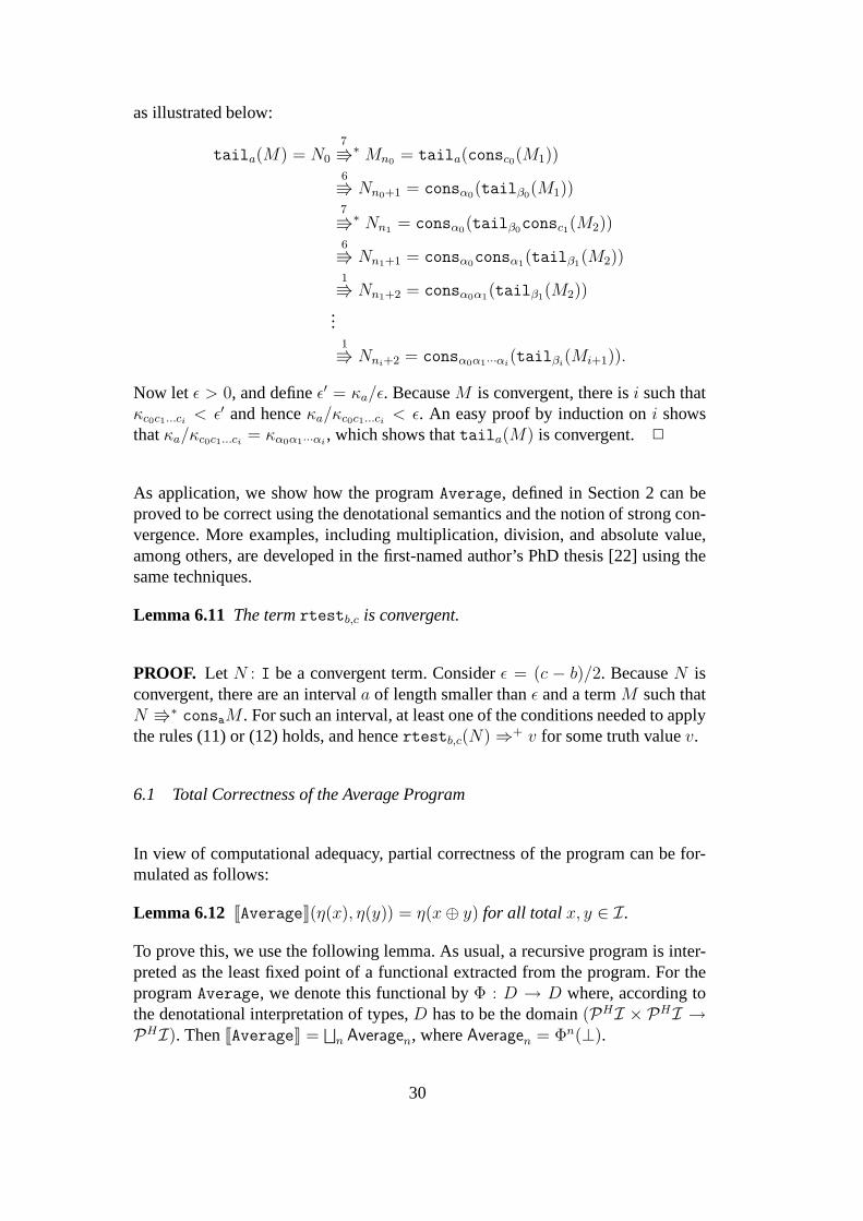
as illustrated below:

taila(M) = N0

7

⇛∗ Mn0

= taila(consc0(M1))6⇛ Nn0+1 = consα0

(tailβ0(M1))

7

⇛∗ Nn1

= consα0(tailβ0

consc1(M2))6⇛ Nn1+1 = consα0

consα1(tailβ1

(M2))1⇛ Nn1+2 = consα0α1

(tailβ1(M2))

...1⇛ Nni+2 = consα0α1···αi

(tailβi(Mi+1)).

Now let ǫ > 0, and defineǫ′ = κa/ǫ. BecauseM is convergent, there isi such thatκc0c1...ci

< ǫ′ and henceκa/κc0c1...ci< ǫ. An easy proof by induction oni shows

thatκa/κc0c1...ci= κα0α1···αi

, which shows thattaila(M) is convergent. 2

As application, we show how the programAverage, defined in Section 2 can beproved to be correct using the denotational semantics and the notion of strong con-vergence. More examples, including multiplication, division, and absolute value,among others, are developed in the first-named author’s PhD thesis [22] using thesame techniques.

Lemma 6.11 The termrtestb,c is convergent.

PROOF. Let N : I be a convergent term. Considerǫ = (c − b)/2. BecauseN isconvergent, there are an intervala of length smaller thanǫ and a termM such thatN ⇛∗ consaM . For such an interval, at least one of the conditions needed to applythe rules (11) or (12) holds, and hencertestb,c(N) ⇒+ v for some truth valuev.

6.1 Total Correctness of the Average Program

In view of computational adequacy, partial correctness of the program can be for-mulated as follows:

Lemma 6.12 JAverageK(η(x), η(y)) = η(x ⊕ y) for all total x, y ∈ I.

To prove this, we use the following lemma. As usual, a recursive program is inter-preted as the least fixed point of a functional extracted fromthe program. For theprogramAverage, we denote this functional byΦ : D → D where, according tothe denotational interpretation of types,D has to be the domain(PHI × PHI →PHI). ThenJAverageK =

⊔n Averagen, whereAveragen = Φn(⊥).

30

Lemma 6.13 For all total x, y ∈ I, the following conditions hold:

(1) JAveragenK(η(x), η(y)) is of the form↓Fn for Fn ⊆ I finite,

(2) κz ≤(

43

)−n+1for eachz ∈ Fn,

(3) Fn ⊑ η(x ⊕ y).

PROOF. The proof is by induction onn.

1.n = 0. We know thatAverage0(η(x), η(y)) = {⊥} = ↓{⊥} for anyx, y ∈ [0, 1].Takez ∈ Fn = {⊥}, soκz = 1 < (4/3)−n+1 = (4/3), and{⊥} ⊑H η(x ⊕ y) forall x, y ∈ [0, 1].

2. Assume that it holds forn. To show that it holds forn+1, we proceed accordingto the position ofx and y relative to the pointsl = 1/4 and r = 3/4 used inthe definition of the average program. All cases are handled in a similar way. Weconsider the casex ≤ 1/4 andy ≤ 1/4 as a representative example.

Averagen+1(η(x), η(y)) = consL(Averagen(tailL(η(x)), tailL(η(y))))

= consL(Averagen(η(tailL(x)), η(tailL(y)))),

and by the induction hypothesis,Averagen(η(t), η(s)) is of the form↓Fn for Fn

finite, t = tailL(x) ands = tailL(y). TakeFn+1 = consL(Fn). Then

Averagen+1(η(x), η(y))

is of the form↓consL(Fn). BecauseFn is finite, so isFn+1.

To show thatκz ≤ (43)−n for anyz ∈ Fn+1, let t ∈ Fn such thatz = consL(t). By

the induction hypothesisκt ≤ (43)−n+1. We havez = consL(t) = 3t

4, and hence

t − t ≤(

4

3

)−n+1

3

4t −

3

4t ≤

(3

4

) (4

3

)−n+1

=(

4

3

)−n

and soκz ≤ (43)−n.

To show thatFn+1 ⊆ η(x ⊕ y), again letz ∈ Fn+1 andt ∈ Fn such that such thatz = consL(t). By the induction hypothesist ∈ η(tailL(x) ⊕ tailL(y)), hence

z = consL(t) ∈ consL(η(tailL(x) ⊕ tailL(y)))

= consL

(η

(4x

3⊕

4y

3

))= consL

(η

(4x + 4y

6

))

= η(consL

(4x + 4y

6

))= η

((3

4

) (4x + 4y

6

))

= η(

x + y

2

)= η(x ⊕ y).

31

as required. 2

To conclude, we establish convergence ofAverage.

Lemma 6.14 For any two convergent termsN1, N2 : I, there are an intervalaof length3/4 and two convergent termsN ′

1, N′2 such thatAverage(N1, N2) ⇛+

consa(Average(N′1, N

′2)).

PROOF. To reduceAverage(N1, N2), we must first unfold the definition, and thenreducertest1/4,3/4(N1), repeatedly applying rule 10, until we get a truth value,which is possible by Lemma 6.11 becauseN1 has been assumed to be convergent.At this point, we have to apply one of the rules 8 or 9. In eithercase, we will nexthave to reducertest1/4,3/4(N2) until it becomes a truth value. Then again one ofthe two rules 8 and 9 will have to be applied, which clearly leads to a term of theform consaAverage(tailb1N1, tailb2N2) with κa = 3/4. By Lemma 6.10, we cantakeN ′

1 = tailb1N1 andN ′2 = tailb2N2. 2

Lemma 6.15 The termAverage is convergent.

PROOF. Let N1 andN2 be convergent terms of typeI. By repeatedly applyingLemma 6.14 and rules 1 and 2, we conclude that for everyn there are an intervalaof length(3/4)n and a termM such thatAverage(N1, N2) ⇛+ consa(M). Herewe use the fact that the length of the interval concatenationbc is the product of thelengths of the intervalsb andc in connection with rule 1. 2

Lemma 6.12 amounts to commutativity of the diagram

I × I ⊂- I × I ⊂- PHI × PHI

I

⊕?

⊂ - I ⊂ - PHI,

JAverageK?

whereI = [0, 1] and the horizontal arrows are the obvious inclusions. The resultsof Escardo, Hofmann and Streicher [9] show that the diagramcannot be completedwith a sequentially computable down arrowI × I → I. Thus, we overcome theproblem by allowing our program to be multi-valued at partial inputs. Lemma 6.13shows that the single-valued output of the program at a totalinput arises as theleast upper bound of multi-valued partial outputs. In otherwords, there are differentcomputation paths that give different, but consistent partial results at finite stages,but all of them converge to the same total real number.

32

Several other examples of recursive definitions, includingmultiplication and di-vision, are developed in [22], with total correctness proofs following the abovepattern.

7 Conclusion and Further Work

Our running example illustrates two important ideas discussed in the introduction:

(1) By considering a multi-valued or non-deterministic construction, it is possibleto have sequential programs for important functions that only admit parallelrealizations in the (singled-valued) interval-domain model, overcoming theproblem identified by Escardo, Hofmann and Streicher [9].

(2) In order to obtain total correctness from partial correctness, a generalization ofthe notion of termination is needed in the case of real-number computations.

Regarding 1, we conjecture that all computable first-order functions are definablein the language. We have some partial results regarding definability of second-order computable functionals such as definite integration.This will be reportedelsewhere, but we remark that the ideas regarding 2 are applied for that purpose.

It is an open problem to find a denotational semantics that would allow to provetotal correctness without the need of resorting to operational methods such as strongconvergence. As we have seen, the Plotkin and Smyth powerdomains cannot beused for that purpose either. In fact, the results of Section4 immediately imply thateven other powerdomains such as the sandwich and the mixed powerdomain cannotbe used. Moreover, it is easy to verify that any of the known powerdomains whichdo not arise as the composition of powerdomains with the Hoare powerdomain asthe last component in the composition are ruled out.

Acknowledgements. We thank Achim Jung, Paul Levy, Steve Vickers and An-drew Moshier for comments and suggestions.

References

[1] Samson Abramsky and Achim Jung, Domain Theory, in: S. Abramsky and D. Gabbayand T. S. E. Maibaum, eds.,Handbook of Logic in Computer Science Volume 3(OxfordUniversity Press, 1994) 1–168.

[2] E. Bishop, and D. Bridges,Constructive Analysis(Springer, Berlin, 1985).

33

[3] H. J. Boehm and R. Cartwright, Exact Real Arithmetic: Formulating Real Numbresas functions, in: Turner. D., editor,Research Topics in Functional Programming(Addison-Wesley 1990) 43–64.

[4] V. Brattka, Recursive characterization of computable real-valued functions andrelations, Theoretical Computer Science162(1996) 45–77.

[5] Peter Buneman and Susan Davidson and Aaron Watters, A semantics for complexobjects and approximate queries,JCSS43 (1991) 170–218.

[6] Abbas Edalat and Peter John Potts and Philipp Sunderhauf, Lazy Computation withExact Real Numbers,International Conference on Functional Programming(1998)185–194.

[7] M. H. Escardo, Real PCF extended with∃ is universal, in: A. Edalat and S. Jourdanand G. McCusker, eds.,Advances in Theory and Formal Methods of Computing:Proceedings of the Third Imperial College Workshop(Christ Church, Oxford, 1996)13–24.

[8] M. H. Escardo PCF extended with real numbers: A domain-theoretic approach tohigher-order exact real number computation,PhD thesis at Imperial College of theUniversity of London1997.

[9] M. H. Escardo and M. Hofmann and Th. Streicher, On the non-sequential nature of theinterval-domain model of exact real-number computation,Mathematical Structures inComputer ScienceAccepted for publication (2002).

[10] M. H. Escardo and Th. Streicher, Induction and recursion on the partial real line withapplications to Real PCF,Theoretical Computer Science210 (1)(1999) 121–157.

[11] M. H. Escardo, PCF Extended with Real Numbers,Theoretical Computer Science162 (1)(1996) 79–115.

[12] A. Farjudian, Sequentiality and Piece-wise affinity inSegments of Real-PCF,Electronic Notes in Theoretical Computer Science73 (2004) 3–4

[13] A. Farjudian, Sequentiality in Real Number Computation, PhD thesis at the Universityof Birmingham2004.

[14] Pietro Di Gianantonio, A Functional Approach to Computability on Real NumbersPhD thesis(Udine, 1993).

[15] Pietro Di Gianantonio, An Abstract Data Type for real numbers,Theoretical ComputerScience221(1999) 295-326

[16] G. Gierz and et al.,Continuous lattices and domains, (Cambridge University Press,2003).

[17] C. A. Gunter, The Mixed Powerdomain,Theoretical Computer Science103 (2)(1992)311–334.

[18] C. A. Gunter and D. S. Scott, Semantic Domains, in: J. vanLeeuwen, editor,Handbook of Theoretical Computer ScienceB (1990) 633–674.

34

[19] Reinhold Heckmann, Power Domain Constructions,Science of ComputerProgramming17 (1-3)(1991) 77–117

[20] H. Luckhardt, A fundamental effect in computations on real numbers,TheoreticalComputer Science5 (3) (1977/78) 321–324.

[21] E. Manes Monads of Sets in: M. Hazewinkel, editor,Handbook of Algebra3 (ElsevierScience, 2003) 67–153.

[22] Jose R. Marcial-Romero, Semantics of a sequential language for exact real-numbercomputation,PhD thesis(Birmingham, December, 2004).

[23] N. Th. Muller, The iRRAM: Exact Arithmetic in C++, in: Blanck, Jens and Brattka,Vasco and Hertling, Peter,Computability and Complexity in Analysis2064(LNCS,2001) 222–252.

[24] D. Normann, Exact real number computations relative tohereditarily total functionals,Theoretical Computer Science284 (2)(2002) 437–453.

[25] G. D. Plotkin, A Powerdomain Construction,SIAM Journal on Computing5 (3)(1976)452–487.

[26] G. D. Plotkin, LCF Considered as a Programming Language, Theoretical ComputerScience5 (1) (1977) 223–255.

[27] G. D. Plotkin, DomainsPost-graduate Lecture in Advanced Domain Theory Univesityof Edinburgh, Departament of Computer Science. Available from the author’s webpage(1983), pages 116.

[28] Peter John Potts and Abbas Edalat and Martın Hotzel Escardo, Semantics of Exact realarithmetic, Proceedings 12th IEEE Symposium on Logic in Computer Science(1997)248–257.

[29] Peter John Potts, Exact real arithmetic using Mobius Transformations,PhD thesis atImperial College of the University of London1998.

[30] Dana Scott, Lattice theory, data type and semantics, in: Randall Rustin, editor, eds.,Formal Semantics of Algorithmic Languages(Prentice Hall, 1972) 65–106.

[31] M. B. Smyth, Power Domains,Journal of Computer and System Science16 (1978)23–36.

[32] M. B. Smyth, Powerdomains and predicate transformers:A topological view ICALP’83, LNCS154(Springer, 1983) 662–675.

[33] M. B. Smyth, Topology, in: S. Abramsky, D. M. Gabbay, andT.S.E Maibaum, eds.,Handbook on Logic in Computer Science1 (1992) 641–761.

[34] S. Vickers, Topolgy via Logic(Cambridge University Press, Cambridge, 1989).

[35] K. Weihrauch,Computable Analysis(Springer-Verlag, 2000) .

35