SemanticKITTI: A Dataset for Semantic Scene Understandingof LiDAR Sequences

Jens Behley∗ Martin Garbade∗ Andres Milioto Jan QuenzelSven Behnke Cyrill Stachniss Juergen Gall

University of Bonn, Germany

www.semantic-kitti.org

Figure 1: Our dataset provides dense annotations for each scan of all sequences from the KITTI Odometry Benchmark [19].Here, we show multiple scans aggregated using pose information estimated by a SLAM approach.

Abstract

Semantic scene understanding is important for variousapplications. In particular, self-driving cars need a fine-grained understanding of the surfaces and objects in theirvicinity. Light detection and ranging (LiDAR) provides pre-cise geometric information about the environment and isthus a part of the sensor suites of almost all self-drivingcars. Despite the relevance of semantic scene understand-ing for this application, there is a lack of a large dataset forthis task which is based on an automotive LiDAR.

In this paper, we introduce a large dataset to propel re-search on laser-based semantic segmentation. We anno-tated all sequences of the KITTI Vision Odometry Bench-mark and provide dense point-wise annotations for the com-plete 360o field-of-view of the employed automotive LiDAR.We propose three benchmark tasks based on this dataset:(i) semantic segmentation of point clouds using a singlescan, (ii) semantic segmentation using multiple past scans,and (iii) semantic scene completion, which requires to an-ticipate the semantic scene in the future. We provide base-line experiments and show that there is a need for moresophisticated models to efficiently tackle these tasks. Ourdataset opens the door for the development of more ad-vanced methods, but also provides plentiful data to inves-tigate new research directions.

∗ indicates equal contribution

1. Introduction

Semantic scene understanding is essential for many ap-plications and an integral part of self-driving cars. Par-ticularly, fine-grained understanding provided by seman-tic segmentation is necessary to distinguish drivable andnon-drivable surfaces and to reason about functional prop-erties, like parking areas and sidewalks. Currently, such un-derstanding, represented in so-called high definition maps,is mainly generated in advance using surveying vehicles.However, self-driving cars should also be able to drivein unmapped areas and adapt their behavior if there arechanges in the environment.

Most self-driving cars currently use multiple differentsensors to perceive the environment. Complementary sen-sor modalities enable to cope with deficits or failures of par-ticular sensors. Besides cameras, light detection and rang-ing (LiDAR) sensors are often used as they provide precisedistance measurements that are not affected by lighting.

Publicly available datasets and benchmarks are crucialfor empirical evaluation of research. They mainly ful-fill three purposes: (i) they provide a basis to measureprogress, since they allow to provide results that are re-producible and comparable, (ii) they uncover shortcomingsof the current state of the art and therefore pave the wayfor novel approaches and research directions, and (iii) theymake it possible to develop approaches without the need tofirst painstakingly collect and label data. While multiple

1

arX

iv:1

904.

0141

6v3

[cs

.CV

] 1

6 A

ug 2

019

#scans1 #points2 #classes3 sensor annotation sequential

SemanticKITTI (Ours) 23201/20351 4549 25 (28) Velodyne HDL-64E point-wise 3

Oakland3d [36] 17 1.6 5 (44) SICK LMS point-wise 7

Freiburg [50, 6] 77 1.1 4 (11) SICK LMS point-wise 7

Wachtberg [6] 5 0.4 5 (5) Velodyne HDL-64E point-wise 7

Semantic3d [23] 15/15 4009 8 (8) Terrestrial Laser Scanner point-wise 7

Paris-Lille-3D [47] 3 143 9 (50) Velodyne HDL-32E point-wise 7

Zhang et al. [66] 140/112 32 10 (10) Velodyne HDL-64E point-wise 7

KITTI [19] 7481/7518 1799 3 Velodyne HDL-64E bounding box 7

Table 1: Overview of other point cloud datasets with semantic annotations. Ours is by far the largest dataset with sequentialinformation. 1Number of scans for train and test set, 2Number of points is given in millions, 3Number of classes used forevaluation and number of classes annotated in brackets.

large datasets for image-based semantic segmentation exist[10, 39], publicly available datasets with point-wise annota-tion of three-dimensional point clouds are still comparablysmall, as shown in Table 1.

To close this gap we propose SemanticKITTI, a largedataset showing unprecedented detail in point-wise annota-tion with 28 classes, which is suited for various tasks. In thispaper, we mainly focus on laser-based semantic segmenta-tion, but also semantic scene completion. The dataset is dis-tinct from other laser datasets as we provide accurate scan-wise annotations of sequences. Overall, we annotated all 22sequences of the odometry benchmark of the KITTI VisionBenchmark [19] consisting of over 43 000 scans. Moreover,we labeled the complete horizontal 360◦ field-of-view ofthe rotating laser sensor. Figure 1 shows example scenesfrom the provided dataset. In summary, our main contribu-tions are:

• We present a point-wise annotated dataset of pointcloud sequences with an unprecedented number ofclasses and unseen level-of-detail for each scan.

• We furthermore provide an evaluation of state-of-the-art methods for semantic segmentation of point clouds.

• We investigate the usage of sequence information forsemantic segmentation using multiple scans.

• Based on the annotation of sequences of a moving car,we furthermore introduce a real-world dataset for se-mantic scene completion and provide baseline results.

• Together with a benchmark website, the point cloudlabeling tool is also publicly available, enabling otherresearchers to generate other labeled datasets in future.

This large dataset will stimulate the development ofnovel algorithms, make it possible to investigate new re-search directions, and puts evaluation and comparison ofthese novel algorithms on a more solid ground.

2. Related Work

The progress of computer vision has always been drivenby benchmarks and datasets [55], but the availability of es-pecially large-scale datasets, such as ImageNet [13], waseven a crucial prerequisite for the advent of deep learning.

More task-specific datasets geared towards self-drivingcars were also proposed. Notable is here the KITTI Vi-sion Benchmark [19] since it showed that off-the-shelf so-lutions are not always suitable for autonomous driving. TheCityscapes dataset [10] is the first dataset for self-drivingcar applications that provides a considerable amount ofpixel-wise labeled images suitable for deep learning. TheMapillary Vistas dataset [39] surpasses the amount and di-versity of labeled data compared to Cityscapes.

Also in point cloud-based interpretation, e.g., semanticsegmentation, RGB-D based datasets enabled tremendousprogress. ShapeNet [8] is especially noteworthy for pointclouds showing a single object, but such data is not directlytransferable to other domains. Specifically, LiDAR sensorsusually do not cover objects as densely as an RGB-D sensordue to their lower angular resolution, in particular in verticaldirection.

For indoor environments, there are several datasets [48,46, 24, 3, 11, 35, 32, 12] available, which are mainlyrecorded using RGB-D cameras or synthetically generated.However, such data shows very different characteristicscompared to outdoor environments, which is also causedby the size of the environment, since point clouds capturedindoors tend to be much denser due to the range at whichobjects are scanned. Furthermore, the sensors have differ-ent properties regarding sparsity and accuracy. While lasersensors are more precise than RGB-D sensors, they usuallyonly capture a sparse point cloud compared to the latter.

For outdoor environments, datasets were recently pro-posed that are recorded with a terrestrial laser scanner(TLS), like the Semantic3d dataset [23], or using automo-tive LiDARs, like the Paris-Lille-3D dataset [47]. However,the Paris-Lille-3D provides only the aggregated scans with

2

point-wise annotations for 50 classes from which 9 are se-lected for evaluation. Another recently used large datasetfor autonomous driving [57], but with fewer classes, is notpublicly available.

The Virtual KITTI dataset [17] provides syntheticallygenerated sequential images with depth information anddense pixel-wise annotation. The depth information canalso be used to generate point clouds. However, these pointclouds do not show the same characteristics as a real rotat-ing LiDAR, including defects like reflections and outliers.

In contrast to these datasets, our dataset combines a largeamount of labeled points, a large variety of classes, and se-quential scans generated by a commonly employed sensorused in autonomous driving, which is distinct from all pub-licly available datasets, also shown in Table 1.

3. The SemanticKITTI DatasetOur dataset is based on the odometry dataset of the

KITTI Vision Benchmark [19] showing inner city traffic,residential areas, but also highway scenes and countrysideroads around Karlsruhe, Germany. The original odome-try dataset consists of 22 sequences, splitting sequences00 to 10 as training set, and 11 to 21 as test set. For con-sistency with the original benchmark, we adopt the samedivision for our training and test set. Moreover, we do notinterfere with the original odometry benchmark by provid-ing labels only for the training data. Overall, we provide23 201 full 3D scans for training and 20 351 for testing,which makes it by a wide margin the largest dataset pub-licly available.

We decided to use the KITTI dataset as a basis for our la-beling effort, since it allowed us to exploit one of the largestavailable collections of raw point cloud data captured with acar. We furthermore expect that there are also potential syn-ergies between our annotations and the existing benchmarksand this will enable the investigation and evaluation of ad-ditional research directions, such as the usage of semanticsfor laser-based odometry estimation.

Compared to other datasets (cf. Table 1), we providelabels for sequential point clouds generated with a com-monly used automotive LiDAR, i.e., the Velodyne HDL-64E. Other publicly available datasets, like Paris-Lille-3D[47] or Wachtberg [6], also use such sensors, but only pro-vide the aggregated point cloud of the whole acquired se-quence or some individual scans of the whole sequence,respectively. Since we provide the individual scans of thewhole sequence, one can also investigate how aggregatingmultiple consecutive scans influences the performance ofthe semantic segmentation and use the information to rec-ognize moving objects.

We annotated 28 classes, where we ensured a large over-lap of classes with the Mapillary Vistas dataset [39] andCityscapes dataset [10] and made modifications where nec-

road sidewalk car

buildingterrainvegetation

other-object

trunk

other-structure

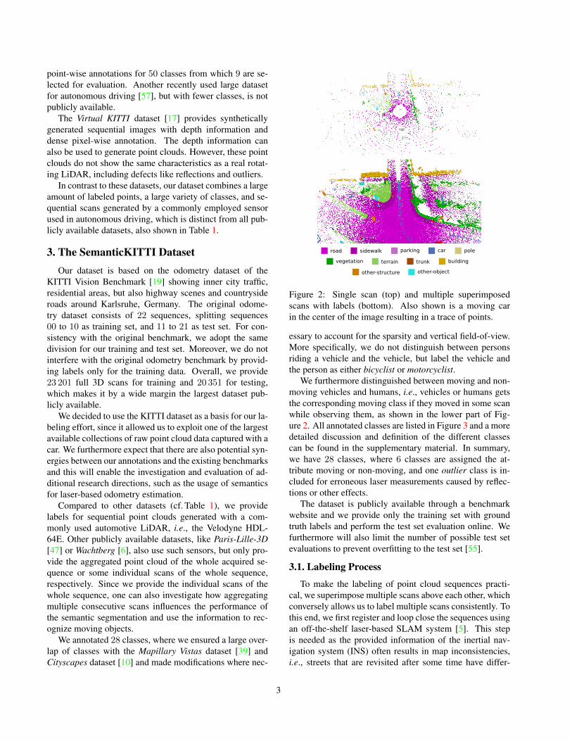
parking pole

Figure 2: Single scan (top) and multiple superimposedscans with labels (bottom). Also shown is a moving carin the center of the image resulting in a trace of points.

essary to account for the sparsity and vertical field-of-view.More specifically, we do not distinguish between personsriding a vehicle and the vehicle, but label the vehicle andthe person as either bicyclist or motorcyclist.

We furthermore distinguished between moving and non-moving vehicles and humans, i.e., vehicles or humans getsthe corresponding moving class if they moved in some scanwhile observing them, as shown in the lower part of Fig-ure 2. All annotated classes are listed in Figure 3 and a moredetailed discussion and definition of the different classescan be found in the supplementary material. In summary,we have 28 classes, where 6 classes are assigned the at-tribute moving or non-moving, and one outlier class is in-cluded for erroneous laser measurements caused by reflec-tions or other effects.

The dataset is publicly available through a benchmarkwebsite and we provide only the training set with groundtruth labels and perform the test set evaluation online. Wefurthermore will also limit the number of possible test setevaluations to prevent overfitting to the test set [55].

3.1. Labeling Process

To make the labeling of point cloud sequences practi-cal, we superimpose multiple scans above each other, whichconversely allows us to label multiple scans consistently. Tothis end, we first register and loop close the sequences usingan off-the-shelf laser-based SLAM system [5]. This stepis needed as the provided information of the inertial nav-igation system (INS) often results in map inconsistencies,i.e., streets that are revisited after some time have differ-

3

ground structure vehicle nature human object105

106

107

108

109

num

ber o

f poi

nts

road

sidew

alk

park

ing

othe

r-gro

und

build

ing

othe

r-stru

ctur

e 1

car

truck

bicy

cle

mot

orcy

cle

othe

r-veh

icle

vege

tatio

n

trunk

terra

in

pers

on

bicy

clist

mot

orcy

clist

fenc

e

pole

traffi

c sig

n

othe

r-obj

ect 1

outli

er 1

1 ignored for evaluation

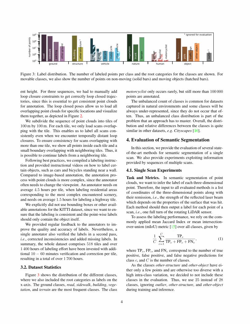
Figure 3: Label distribution. The number of labeled points per class and the root categories for the classes are shown. Formovable classes, we also show the number of points on non-moving (solid bars) and moving objects (hatched bars).

ent height. For three sequences, we had to manually addloop closure constraints to get correctly loop closed trajec-tories, since this is essential to get consistent point cloudsfor annotation. The loop closed poses allow us to load alloverlapping point clouds for specific locations and visualizethem together, as depicted in Figure 2.

We subdivide the sequence of point clouds into tiles of100m by 100m. For each tile, we only load scans overlap-ping with the tile. This enables us to label all scans con-sistently even when we encounter temporally distant loopclosures. To ensure consistency for scans overlapping withmore than one tile, we show all points inside each tile and asmall boundary overlapping with neighboring tiles. Thus, itis possible to continue labels from a neighboring tile.

Following best practices, we compiled a labeling instruc-tion and provided instructional videos on how to label cer-tain objects, such as cars and bicycles standing near a wall.Compared to image-based annotation, the annotation pro-cess with point clouds is more complex, since the annotatoroften needs to change the viewpoint. An annotator needs onaverage 4.5 hours per tile, when labeling residential areascorresponding to the most complex encountered scenery,and needs on average 1.5 hours for labeling a highway tile.

We explicitly did not use bounding boxes or other avail-able annotations for the KITTI dataset, since we want to en-sure that the labeling is consistent and the point-wise labelsshould only contain the object itself.

We provided regular feedback to the annotators to im-prove the quality and accuracy of labels. Nevertheless, asingle annotator also verified the labels in a second pass,i.e., corrected inconsistencies and added missing labels. Insummary, the whole dataset comprises 518 tiles and over1 400 hours of labeling effort have been invested with addi-tional 10 − 60 minutes verification and correction per tile,resulting in a total of over 1 700 hours.

3.2. Dataset Statistics

Figure 3 shows the distribution of the different classes,where we also included the root categories as labels on thex-axis. The ground classes, road, sidewalk, building, vege-tation, and terrain are the most frequent classes. The class

motorcyclist only occurs rarely, but still more than 100 000points are annotated.

The unbalanced count of classes is common for datasetscaptured in natural environments and some classes will bealways under-represented, since they do not occur that of-ten. Thus, an unbalanced class distribution is part of theproblem that an approach has to master. Overall, the distri-bution and relative differences between the classes is quitesimilar in other datasets, e.g. Cityscapes [10].

4. Evaluation of Semantic SegmentationIn this section, we provide the evaluation of several state-

of-the-art methods for semantic segmentation of a singlescan. We also provide experiments exploiting informationprovided by sequences of multiple scans.

4.1. Single Scan Experiments

Task and Metrics. In semantic segmentation of pointclouds, we want to infer the label of each three-dimensionalpoint. Therefore, the input to all evaluated methods is a listof coordinates of the three-dimensional points along withtheir remission, i.e., the strength of the reflected laser beamwhich depends on the properties of the surface that was hit.Each method should then output a label for each point of ascan, i.e., one full turn of the rotating LiDAR sensor.

To assess the labeling performance, we rely on the com-monly applied mean Jaccard Index or mean intersection-over-union (mIoU) metric [15] over all classes, given by

1

C

C∑c=1

TPc

TPc + FPc + FNc, (1)

where TPc, FPc, and FNc correspond to the number of truepositive, false positive, and false negative predictions forclass c, and C is the number of classes.

As the classes other-structure and other-object have ei-ther only a few points and are otherwise too diverse with ahigh intra-class variation, we decided to not include theseclasses in the evaluation. Thus, we use 25 instead of 28classes, ignoring outlier, other-structure, and other-objectduring training and inference.

4

Furthermore, we cannot expect to distinguish movingfrom non-moving objects with a single scan, since this Velo-dyne LiDAR cannot measure velocities like radars exploit-ing the Doppler effect. We therefore combine the movingclasses with the corresponding non-moving class resultingin a total number of 19 classes for training and evaluation.

State of the Art. Semantic segmentation or point-wiseclassification of point clouds is a long-standing topic [2],which was traditionally solved using a feature extractor,such as Spin Images [29], in combination with a traditionalclassifier, like support vector machines [1] or even semantichashing [4]. Many approaches used Conditional RandomFields (CRF) to enforce label consistency of neighboringpoints [56, 37, 36, 38, 63].

With the advent of deep learning approaches in image-based classification, the whole pipeline of feature extrac-tion and classification has been replaced by end-to-end deepneural networks. Voxel-based methods transforming thepoint cloud into a voxel-grid and then applying convolu-tional neural networks (CNN) with 3D convolutions for ob-ject classification [34] and semantic segmentation [26] wereamong the first investigated models, since they allowed toexploit architectures and insights known for images.

To overcome the limitations of the voxel-based represen-tation, such as the exploding memory consumption whenthe resolution of the voxel grid increases, more recent ap-proaches either upsample voxel-predictions [53] using aCRF or use different representations, like more efficientspatial subdivisions [30, 44, 64, 59, 21], rendered 2D im-age views [7], graphs [31, 54], splats [51], or even directlythe points [41, 40, 25, 22, 43, 28, 14].

Baseline approaches. We provide the results of six state-of-the-art architectures for the semantic segmentation ofpoint clouds in our dataset: PointNet [40], PointNet++ [41],Tangent Convolutions [52], SPLATNet [51], SuperpointGraph [31], and SqueezeSeg (V1 and V2) [60, 61]. Further-more, we investigate two extensions of SqueezeSeg: Dark-Net21Seg and DarkNet53Seg.

PointNet [40] and PointNet++ [41] use the raw un-ordered point cloud data as input. Core of these approachesis max pooling to get an order-invariant operator that workssurprisingly well for semantic segmentation of shapes andseveral other benchmarks. Due to this nature, however,PointNet fails to capture the spatial relationships betweenthe features. To alleviate this, PointNet++ [41] applies indi-vidual PointNets to local neighborhoods and uses a hierar-chical approach to combine their outputs. This enables it tobuild complex hierarchical features that capture both localfine-grained and global contextual information.

Tangent Convolutions [52] also handles unstructuredpoint clouds by applying convolutional neural networks di-rectly on surfaces. This is achieved by assuming that the

data is sampled from smooth surfaces and defining a tan-gent convolution as a convolution applied to the projectionof the local surface at each point into the tangent plane.

SPLATNet [51] takes an approach that is similar to theaforementioned voxelization methods and represents thepoint clouds in a high-dimensional sparse lattice. As withvoxel-based methods, this scales poorly both in compu-tation and in memory cost and therefore they exploit thesparsity of this representation by using bilateral convolu-tions [27], which only operates on occupied lattice parts.

Similarly to PointNet, Superpoint Graph [31], capturesthe local relationships by summarizing geometrically ho-mogeneous groups of points into superpoints, which arelater embedded by local PointNets. The result is a super-point graph representation that is more compact and richthan the original point cloud exploiting contextual relation-ships between the superpoints.

SqueezeSeg [60, 61] also discretizes the point cloud ina way that makes it possible to apply 2D convolutions tothe point cloud data exploiting the sensor geometry of a ro-tating LiDAR. In the case of a rotating LiDAR, all pointsof a single turn can be projected to an image by using aspherical projection. A fully convolutional neural networkis applied and then finally filtered with a CRF to smooththe results. Due to the promising results of SqueezeSeg andthe fast training, we investigated how the labeling perfor-mance is affected by the number of model parameters. Tothis end, we used a different backbone based on the Dark-net architecture [42] with 21 and 53 layers, and 25 and 50million parameters respectively. We furthermore eliminatedthe vertical downsampling used in the architecture.

We modified the available implementations such that themethods could be trained and evaluated on our large-scaledataset. Note that most of these approaches have so far onlybeen evaluated on shape [8] or RGB-D indoor datasets [48].However, some of the approaches [40, 41] were only possi-ble to run with considerable downsampling to 50 000 pointsdue to memory limitations.

Results and Discussion. Table 2 shows the results of ourbaseline experiments for various approaches using either di-rectly the point cloud information [40, 41, 51, 52, 31] or aprojection of the point cloud [60]. The results show that thecurrent state of the art for point cloud semantic segmenta-tion falls short for the size and complexity of our dataset.

We believe that this is mainly caused by the limited ca-pacity of the used architectures (see Table 7), because thenumber of parameters of these approaches is much lowerthan the number of parameters used in leading image-basedsemantic segmentation networks. As mentioned above, weadded DarkNet21Seg and DarkNet53Seg to test this hy-pothesis and the results show that this simple modifica-tion improves the accuracy from 29.5% for SqueezeSeg to47.4% for DarkNet21Seg and to 49.9% for DarkNet53Seg.

5

Approach mIo

U

road

side

wal

k

park

ing

othe

r-gr

ound

build

ing

car

truc

k

bicy

cle

mot

orcy

cle

othe

r-ve

hicl

e

vege

tatio

n

trun

k

terr

ain

pers

on

bicy

clis

t

mot

orcy

clis

t

fenc

e

pole

traf

ficsi

gn

PointNet [40] 14.6 61.6 35.7 15.8 1.4 41.4 46.3 0.1 1.3 0.3 0.8 31.0 4.6 17.6 0.2 0.2 0.0 12.9 2.4 3.7SPGraph [31] 17.4 45.0 28.5 0.6 0.6 64.3 49.3 0.1 0.2 0.2 0.8 48.9 27.2 24.6 0.3 2.7 0.1 20.8 15.9 0.8SPLATNet [51] 18.4 64.6 39.1 0.4 0.0 58.3 58.2 0.0 0.0 0.0 0.0 71.1 9.9 19.3 0.0 0.0 0.0 23.1 5.6 0.0PointNet++ [41] 20.1 72.0 41.8 18.7 5.6 62.3 53.7 0.9 1.9 0.2 0.2 46.5 13.8 30.0 0.9 1.0 0.0 16.9 6.0 8.9SqueezeSeg [60] 29.5 85.4 54.3 26.9 4.5 57.4 68.8 3.3 16.0 4.1 3.6 60.0 24.3 53.7 12.9 13.1 0.9 29.0 17.5 24.5SqueezeSegV2 [61] 39.7 88.6 67.6 45.8 17.7 73.7 81.8 13.4 18.5 17.9 14.0 71.8 35.8 60.2 20.1 25.1 3.9 41.1 20.2 36.3TangentConv [52] 40.9 83.9 63.9 33.4 15.4 83.4 90.8 15.2 2.7 16.5 12.1 79.5 49.3 58.1 23.0 28.4 8.1 49.0 35.8 28.5DarkNet21Seg 47.4 91.4 74.0 57.0 26.4 81.9 85.4 18.6 26.2 26.5 15.6 77.6 48.4 63.6 31.8 33.6 4.0 52.3 36.0 50.0DarkNet53Seg 49.9 91.8 74.6 64.8 27.9 84.1 86.4 25.5 24.5 32.7 22.6 78.3 50.1 64.0 36.2 33.6 4.7 55.0 38.9 52.2

Table 2: Single scan results (19 classes) for all baselines on sequences 11 to 21 (test set). All methods were trained onsequences 00 to 10, except for sequence 08 which is used as validation set.

10 15 20 25 30 35 40 45 50Distance to sensor [m]

10

20

30

40

Mea

n Io

U [%

]

PointNetPointNet++SPGraph

SPLATNetTangentConvSqueezeSeg

SqueezeSegV2DarkNet21SegDarkNet53Seg

Figure 4: IoU vs. distance to the sensor.

Another reason is that the point clouds generated by Li-DAR are relatively sparse, especially as the distance to thesensor increases. This is partially solved in SqueezeSeg,which exploits the way the rotating scanner captures thedata to generate a dense range image, where each pixel cor-responds roughly to a point in the scan.

These effects are further analyzed in Figure 4, where themIoU is plotted w.r.t. the distance to the sensor. It showsthat results of all approaches get worse with increasing dis-tance. This further confirms our hypothesis that the spar-sity is the main reason for worse results at large distances.However, the results also show that some methods, like SP-Graph, are less affected by the distance-dependent sparsityand this might be a promising direction for future researchto combine the strength of both paradigms.

Especially classes with few examples, like motorcyclistsand trucks, seem to be more difficult for all approaches. Butalso classes with only a small number of points in a singlepoint cloud, like bicycles and poles, are hard classes.

Finally, the best performing approach (DarkNet53Seg)with 49.9% mIoU is still far from achieving results thatare on par with image-based approaches, e.g., 80% on theCityscapes benchmark [10].

Approach num. parameters train time inference time

(million)(

GPU hoursepoch

) (seconds

point cloud

)PointNet 3 4 0.5PointNet++ 6 16 5.9SPGraph 0.25 6 5.2TangentConv 0.4 6 3.0SPLATNet 0.8 8 1.0SqueezeSeg 1 0.5 0.015SqueezeSegV2 1 0.6 0.02DarkNet21Seg 25 2 0.055DarkNet53Seg 50 3 0.1

Table 3: Approach statistics.

4.2. Multiple Scan Experiments

Task and Metrics. In this task, we allow methods to ex-ploit information from a sequence of multiple past scansto improve the segmentation of the current scan. We fur-thermore want the methods to distinguish moving and non-moving classes, i.e., all 25 classes must be predicted, sincethis information should be visible in the temporal informa-tion of multiple past scans. The evaluation metric for thistask is still the same as in the single scan case, i.e., we eval-uate the mean IoU of the current scan no matter how manypast scans were used to compute the results.

Baselines. We exploit the sequential information by com-bining 5 scans into a single, large point cloud, i.e., the cur-rent scan at timestamp t and the 4 scans before at times-tamps t− 1, . . . , t− 4. We evaluate DarkNet53Seg andTangentConv, since these approaches can deal with a largernumber of points without downsampling of the point cloudsand could still be trained in a reasonable amount of time.

Results and Discussion. Table 4 shows the per-class re-sults for the movable classes and the mean IoU (mIoU) overall classes. For each method, we show in the upper part ofthe row the IoU for non-moving (unshaded) and in the lowerpart of the row the IoU for moving objects (shaded). The

6

Approach car

truc

k

othe

r-ve

hicl

e

pers

on

bicy

clis

t

mot

orcy

clis

t

mIo

U

TangentConv [52] 84.9 21.1 18.5 1.6 0.0 0.0 34.140.3 42.2 30.1 6.4 1.1 1.9

DarkNet53Seg 84.1 20.0 20.7 7.5 0.0 0.0 41.661.5 37.8 28.9 15.2 14.1 0.2

Table 4: IoU results using a sequence of multiple past scans(in %). Shaded cells correspond to the IoU of the movingclasses, while unshaded entries are the non-moving classes.

performance of the remaining static classes is similar to thesingle scan results and we refer to the supplement for a tablecontaining all classes.

The general trend that the projective methods performbetter than the point-based methods is still apparent, whichcan be also attributed to the larger amount of parametersas in the single scan case. Both approaches show difficul-ties in separating moving and non-moving objects, whichmight be caused by our design decision to aggregate multi-ple scans into a single large point cloud. The results showthat especially bicyclist and motorcyclist never get correctlyassigned the non-moving class, which is most likely a con-sequence from the generally sparser object point clouds.

We expect that new approaches could explicitly exploitthe sequential information by using multiple input streamsto the architecture or even recurrent neural networks to ac-count for the temporal information, which again might opena new line of research.

5. Evaluation of Semantic Scene Completion

After leveraging a sequence of past scans for seman-tic point cloud segmentation, we now show a scenario thatmakes use of future scans. Due to its sequential nature, ourdataset provides the unique opportunity to be extended forthe task of 3D semantic scene completion. Note that this isthe first real world outdoor benchmark for this task. Exist-ing point cloud datasets cannot be used to address this task,as they do not allow for aggregating labeled point cloudsthat are sufficiently dense in both space and time.

In semantic scene completion, one fundamental prob-lem is to obtain ground truth labels for real world datasets.In case of NYUv2 [48], CAD models were fit into thescene [45] using an RGB-D image captured by a Kinectsensor. New approaches often resort to prove their effective-ness on the larger, but synthetic SUNCG dataset [49]. How-ever, a dataset combining the scale of a synthetic dataset andusage of real-world data is still missing.

In the case of our proposed dataset, the car carrying theLiDAR moves past 3D objects in the scene and thereby

records their backsides, which are hidden in the initialscan due to self-occlusion. This is exactly the informationneeded for semantic scene completion as it contains the full3D geometry of all objects while their semantics are pro-vided by our dense annotations.

Dataset Generation. By superimposing an exhaustivenumber of future laser scans in a predefined region in frontof the car, we can generate pairs of inputs and targets thatcorrespond to the task of semantic scene completion. Asproposed by Song et al. [49], our dataset for the scene com-pletion task is a voxelized representation of the 3D scene.

We select a volume of 51.2m ahead of the car, 25.6mto every side and 6.4m in height with a voxel resolution of0.2m, which results in a volume of 256×256×32 voxels topredict. We assign a single label to every voxel based on themajority vote over all labeled points inside a voxel. Voxelsthat do not contain any points are labeled as empty.

To compute which voxels belong to the occluded space,we check for every pose of the car which voxels are visi-ble to the sensor by tracing a ray. Some of the voxels, e.g.those inside objects or behind walls are never visible, so weignore them during training and evaluation.

Overall, we extracted 19 130 pairs of input and targetvoxel grids for training, 815 for validation and 3 992 fortesting. For the test set, we only provide the unlabeled in-put voxel grid and withhold the target voxel grids. Figure 5shows an example of an input and target pair.

Task and Metrics. In semantic scene completion, we areinterested in predicting the complete scene inside a certainvolume from a single initial scan. More specifically, we useas input a voxel grid, where each voxel is marked as emptyor occupied, depending on whether or not it contains a lasermeasurement. For semantic scene completion, one needs topredict whether a voxel is occupied and its semantic labelin the completed scene.

For evaluation, we follow the evaluation protocol ofSong et al. [49] and compute the IoU for the task of scenecompletion, which only classifies a voxel as being occu-pied or empty, i.e., ignoring the semantic label, as well asmIoU (1) for the task of semantic scene completion over thesame 19 classes that were used for the single scan semanticsegmentation task (see Section 4).

State of the Art. Early approaches addressed the task ofscene completion either without predicting semantics [16],thereby not providing a holistic understanding of the scene,or by trying to fit a fixed number of mesh models to thescene geometry [20], which limits the expressiveness of theapproach.

Song et al. [49] were the first to address the task of se-mantic scene completion in an end-to-end fashion. Theirwork spawned a lot of interest in the field yielding mod-els that combine the usage of color and depth informa-

7

Figure 5: Left: Visualization of the incomplete input for the semantic scene completion benchmark. Note that we show thelabels only for better visualization, but the real input is a single raw voxel grid without any labels. Right: Correspondingtarget output representing the completed and fully labeled 3D scene.

tion [33, 18] or address the problem of sparse 3D fea-ture maps by introducing submanifold convolutions [65] orincrease the output resolution by deploying a multi-stagecoarse to fine training scheme [12]. Other works exper-imented with new encoder-decoder CNN architectures aswell as improving the loss term by adding adversarial losscomponents [58].

Baseline Approaches. We report the results of four se-mantic scene completion approaches. In the first approach,we apply SSCNet [49] without the flipped TSDF as inputfeature. This has minimal impact on the performance, butsignificantly speeds up the training time due to faster pre-processing [18]. Then we use the Two Stream (TS3D) ap-proach [18], which makes use of the additional informationfrom the RGB image corresponding to the input laser scan.Therefore the RGB image is first processed by a 2D seman-tic segmentation network, using the approach DeepLab v2(ResNet-101) [9] trained on Cityscapes to generate a se-mantic segmentation. The depth information from the sin-gle laser scan and the labels inferred from the RGB imageare combined in an early fusion. Furthermore, we modifythe TS3D approach in two steps: First, by directly usinglabels from the best LiDAR-based semantic segmentationapproach (DarkNet53Seg) and secondly, by exchanging the3D-CNN backbone by SATNet [33].

Results and Discussion. Table 5 shows the results of eachof the baselines, whereas results for individual classes arereported in the supplement. The TS3D network, incorpo-rating 2D semantic segmentation of the RGB image, per-forms similar to SSCNet which only uses depth informa-tion. However, the usage of the best semantic segmen-tation directly working on the point cloud slightly out-performs SSCNet on semantic scene completion (TS3D +DarkNet53Seg). Note that the first three approaches arebased on SSCNet’s 3D-CNN architecture, which performsa 4 fold downsampling in a forward pass and thus rendersthem incapable of dealing with details of the scene. Inour final approach, we exchange the SSCNet-backbone ofTS3D + DarkNet53Seg with SATNet [33], which is capa-ble of dealing with the desired output resolution. Due to

Completion Semantic Scene(IoU) Completion (mIoU)

SSCNet [49] 29.83 9.53TS3D [18] 29.81 9.54TS3D [18] + DarkNet53Seg 24.99 10.19TS3D [18] + DarkNet53Seg + SATNet 50.60 17.70

Table 5: Semantic scene completion baselines.

memory limitations, we use random cropping during train-ing. During inference, we divide each volume into six equalparts, perform scene completion on them individually andsubsequently fuse them. This approach performs much bet-ter than the SSCNet based approaches.

Apart from dealing with the target resolution, a challengefor current models is the sparsity of the laser input signal inthe far field as can be seen from Figure 5. To obtain a higherresolution input signal in the far field, approaches wouldhave to exploit more efficiently information from high res-olution RGB images provided along with each laser scan.

6. Conclusion and OutlookIn this work, we have presented a large-scale dataset

showing unprecedented scale in point-wise annotation ofpoint cloud sequences. We provide a range of differentbaseline experiments for three tasks: (i) semantic segmen-tation using a single scan, (ii) semantic segmentation usingmultiple scans, and (iii) semantic scene completion.

In future work, we plan to provide also instance-levelannotation over the whole sequence, i.e., we want to distin-guish different objects in a scan, but also identify the sameobject over time. This will enable to investigate temporalinstance segmentation over sequences. However, we alsosee potential for other new tasks based on our labeling ef-fort, such as the evaluation of semantic SLAM.

Acknowledgments We thank all students that helped withannotating the data. The work has been funded by the DeutscheForschungsgemeinschaft (DFG, German Research Founda-tion) under FOR 1505 Mapping on Demand, BE 5996/1-1,GA 1927/2-2, and under Germanys Excellence Strategy, EXC-2070 – 390732324 (PhenoRob).

8

References[1] Anuraag Agrawal, Atsushi Nakazawa, and Haruo Takemura.

MMM-classification of 3D Range Data. In Proc. of the IEEEIntl. Conf. on Robotics & Automation (ICRA), 2009. 5

[2] Dragomir Anguelov, Ben Taskar, Vassil Chatalbashev,Daphne Koller, Dinkar Gupta, Geremy Heitz, and AndrewNg. Discriminative Learning of Markov Random Fieldsfor Segmentation of 3D Scan Data. In Proc. of the IEEEConf. on Computer Vision and Pattern Recognition (CVPR),pages 169–176, 2005. 5

[3] Iro Armeni, Alexander Sax, Amir R. Zamir, and SilvioSavarese. Joint 2D-3D-Semantic Data for Indoor Scene Un-derstanding. arXiv preprint, 2017. 2

[4] Jens Behley, Kristian Kersting, Dirk Schulz, Volker Stein-hage, and Armin B. Cremers. Learning to Hash LogisticRegression for Fast 3D Scan Point Classification. In Proc. ofthe IEEE/RSJ Intl. Conf. on Intelligent Robots and Systems(IROS), pages 5960–5965, 2010. 5

[5] Jens Behley and Cyrill Stachniss. Efficient Surfel-BasedSLAM using 3D Laser Range Data in Urban Environments.In Proc. of Robotics: Science and Systems (RSS), 2018. 3

[6] Jens Behley, Volker Steinhage, and Armin B. Cremers. Per-formance of Histogram Descriptors for the Classification of3D Laser Range Data in Urban Environments. In Proc. of theIEEE Intl. Conf. on Robotics & Automation (ICRA), 2012. 2,3

[7] Alexandre Boulch, Joris Guerry, Bertrand Le Saux, andNicolas Audebert. SnapNet: 3D point cloud semantic la-beling with 2D deep segmentation networks. Computers &Graphics, 2017. 5

[8] Angel X. Chang, Thomas Funkhouser, Leonidas J. Guibas,Pat Hanrahan, Qixing Huang, Zimo Li, Silvio Savarese,Manolis Savva, Shuran Song, Hao Su, Jianxiong Xiao, Li Yi,and Fisher Yu. ShapeNet: An Information-Rich 3D ModelRepository. Technical Report arXiv:1512.03012 [cs.GR],Stanford University and Princeton University and ToyotaTechnological Institute at Chicago, 2015. 2, 5

[9] Liang-Chieh Chen, George Papandreou, Iasonas Kokkinos,Kevin Murphy, and Alan L. Yuille. DeepLab: SemanticImage Segmentation withDeep Convolutional Nets, AtrousConvolution,and Fully Connected CRFs. IEEE Transac-tions on Pattern Analysis and Machine Intelligence (PAMI),40(4):834–848, 2018. 8, 14

[10] Marius Cordts, Mohamed Omran, Sebastian Ramos, TimoRehfeld, Markus Enzweiler, Rodrigo Benenson, UweFranke, Stefan Roth, and Bernt Schiele. The CityscapesDataset for Semantic Urban Scene Understanding. InProc. of the IEEE Conf. on Computer Vision and PatternRecognition (CVPR), 2016. 2, 3, 4, 6, 12, 14

[11] Angela Dai, Angel X. Chang, Manolis Savva, Maciej Hal-ber, Thomas Funkhouser, and Matthias Nießner. ScanNet:Richly-annotated 3D Reconstructions of Indoor Scenes. InProc. of the IEEE Conf. on Computer Vision and PatternRecognition (CVPR), 2009. 2

[12] Angela Dai, Daniel Ritchie, Martin Bokeloh, Scott Reed,Jurgen Sturm, and Matthias Nießner. ScanComplete: Large-Scale Scene Completion and Semantic Segmentation for 3D

Scans. In Proc. of the IEEE Conf. on Computer Vision andPattern Recognition (CVPR), 2018. 2, 8

[13] Jia Deng, Wei Dong, Richard Socher, Li-Jia Li, Kai Li, andLi Fei-Fei. ImageNet: A Large-Scale Hierarchical ImageDatabase. In Proc. of the IEEE Conf. on Computer Visionand Pattern Recognition (CVPR), 2009. 2

[14] Francis Engelmann, Theodora Kontogianni, Jonas Schult,and Bastian Leibe. Know What Your Neighbors Do: 3D Se-mantic Segmentation of Point Clouds. arXiv preprint, 2018.5

[15] Mark Everingham, S.M. Ali Eslami, Luc van Gool, Christo-pher K.I. Williams, John Winn, and Andrew Zisserman. ThePascal Visual Object Classes Challenge a Retrospective. In-ternational Journal on Computer Vision (IJCV), 111(1):98–136, 2015. 4

[16] Michael Firman, Oisin Mac Aodha, Simon Julier, andGabriel J. Brostow. Structured Prediction of UnobservedVoxels From a Single Depth Image. In Proc. of the IEEEConf. on Computer Vision and Pattern Recognition (CVPR),pages 5431–5440, 2016. 7

[17] Adrien Gaidon, Qiao Wang, Yohann Cabon, and EleonoraVig. Virtual Worlds as Proxy for Multi-Object TrackingAnalysis. In Proc. of the IEEE Conf. on Computer Visionand Pattern Recognition (CVPR), 2016. 3

[18] Martin Garbade, Yueh-Tung Chen, J. Sawatzky, and Juer-gen Gall. Two Stream 3D Semantic Scene Completion. InProc. of the IEEE/CVF Conf. on Computer Vision and Pat-tern Recognition (CVPR) Workshops, 2019. 7, 8

[19] Andreas Geiger, Philip Lenz, and Raquel Urtasun. Are weready for Autonomous Driving? The KITTI Vision Bench-mark Suite. In Proc. of the IEEE Conf. on Computer Visionand Pattern Recognition (CVPR), pages 3354–3361, 2012.1, 2, 3, 12

[20] Andres Geiger and Chaohui Wang. Joint 3d Object and Lay-out Inference from a single RGB-D Image. In Proc. of theGerman Conf. on Pattern Recognition (GCPR), pages 183–195, 2015. 7

[21] Benjamin Graham, Martin Engelcke, and Laurens van derMaaten. 3D Semantic Segmentation with SubmanifoldSparse Convolutional Networks. In Proc. of the IEEEConf. on Computer Vision and Pattern Recognition (CVPR),2018. 5

[22] Fabian Groh, Patrick Wieschollek, and Hendrik Lensch.Flex-Convolution (Million-Scale Pointcloud Learning Be-yond Grid-Worlds). In Proc. of the Asian Conf. on ComputerVision (ACCV), Dezember 2018. 5

[23] Timo Hackel, Nikolay Savinov, Lubor Ladicky, Jan D.Wegner, Konrad Schindler, and Marc Pollefeys. SEMAN-TIC3D.NET: A new large-scale point cloud classificationbenchmark. In ISPRS Annals of the Photogrammetry, Re-mote Sensing and Spatial Information Sciences, volume IV-1-W1, pages 91–98, 2017. 2

[24] Binh-Son Hua, Quang-Hieu Pham, Duc Thanh Nguyen,Minh-Khoi Tran, Lap-Fai Yu, and Sai-Kit Yeung. SceneNN:A Scene Meshes Dataset with aNNotations. In Proc. of theIntl. Conf. on 3D Vision (3DV), 2016. 2

[25] Binh-Son Hua, Minh-Khoi Tran, and Sai-Kit Yeung. Point-wise Convolutional Neural Networks. In Proc. of the IEEE

9

Conf. on Computer Vision and Pattern Recognition (CVPR),2018. 5

[26] Jing Huang and Suya You. Point Cloud Labeling using 3DConvolutional Neural Network. In Proc. of the Intl. Conf. onPattern Recognition (ICPR), 2016. 5

[27] Varun Jampani, Martin Kiefel, and Peter V. Gehler. Learn-ing Sparse High Dimensional Filters: Image Filtering, DenseCRFs and Bilateral Neural Networks. In Proc. of the IEEEConf. on Computer Vision and Pattern Recognition (CVPR),2016. 5

[28] Mingyang Jiang, Yiran Wu, and Cewu Lu. PointSIFT: ASIFT-like Network Module for 3D Point Cloud SemanticSegmentation. arXiv preprint, 2018. 5

[29] Andrew E. Johnson and Martial Hebert. Using spinimages for effcient object recognition in cluttered 3Dscenes. Trans. on Pattern Analysis and Machine Intelligence(TPAMI), 21(5):433–449, 1999. 5

[30] Roman Klukov and Victor Lempitsky. Escape from Cells:Deep Kd-Networks for the Recognition of 3D Point CloudModels. In Proc. of the IEEE Intl. Conf. on Computer Vision(ICCV), 2017. 5

[31] Loic Landrieu and Martin Simonovsky. Large-scale PointCloud Semantic Segmentation with Superpoint Graphs. InProc. of the IEEE Conf. on Computer Vision and PatternRecognition (CVPR), 2018. 5, 6, 15

[32] Wenbin Li, Sajad Saeedi, John McCormac, Ronald Clark,Dimos Tzoumanikas, Qing Ye, Yuzhong Huang, Rui Tang,and Stefan Leutenegger. InteriorNet: Mega-scale Multi-sensor Photo-realistic Indoor Scenes Dataset. In Proc. of theBritish Machine Vision Conference (BMVC), 2018. 2

[33] Shice Liu, Yu Hu, Yiming Zeng, Qiankun Tang, Beibei Jin,Yainhe Han, and Xiaowei Li. See and Think: DisentanglingSemantic Scene Completion. In Proc. of the Conf. on NeuralInformation Processing Systems (NeurIPS), pages 261–272,2018. 7, 8

[34] Daniel Maturana and Sebastian Scherer. VoxNet: A 3D Con-volutional Neural Network for Real-Time Object Recogni-tion. In Proc. of the IEEE/RSJ Intl. Conf. on IntelligentRobots and Systems (IROS), 2015. 5

[35] John McCormac, Ankur Handa, Stefan Leutenegger, andAndrew J. Davison. SceneNet RGB-D: Can 5M SyntheticImages Beat Generic ImageNet Pre-training on Indoor Seg-mentation? In Proc. of the IEEE Intl. Conf. on ComputerVision (ICCV), 2017. 2

[36] Daniel Munoz, J. Andrew Bagnell, Nicolas Vandapel, andMartial Hebert. Contextual Classification with FunctionalMax-Margin Markov Networks. In Proc. of the IEEEConf. on Computer Vision and Pattern Recognition (CVPR),2009. 2, 5

[37] Daniel Munoz, Nicholas Vandapel, and Marial Hebert. Di-rectional Associative Markov Network for 3-D Point CloudClassification. In Proc. of the International Symposiumon 3D Data Processing, Visualization and Transmission(3DPVT), pages 63–70, 2008. 5

[38] Daniel Munoz, Nicholas Vandapel, and Martial Hebert. On-board Contextual Classification of 3-D Point Clouds withLearned High-order Markov Random Fields. In Proc. of theIEEE Intl. Conf. on Robotics & Automation (ICRA), 2009. 5

[39] Gerhard Neuhold, Tobias Ollmann, Samuel Rota Bulo, andPeter Kontschieder. The Mapillary Vistas Dataset for Se-mantic Understanding of Street Scenes. In Proc. of the IEEEIntl. Conf. on Computer Vision (ICCV), 2017. 2, 3, 12

[40] Charles R. Qi, Hao Su, Kaichun Mo, and Leonidas J. Guibas.PointNet: Deep Learning on Point Sets for 3D Classificationand Segmentation. In Proc. of the IEEE Conf. on ComputerVision and Pattern Recognition (CVPR), 2017. 5, 6, 14, 15

[41] Charles R. Qi, Li Yi, Hao Su, and Leonidas J. Guibas. Point-Net++: Deep Hierarchical Feature Learning on Point Sets ina Metric Space. In Proc. of the Conf. on Neural InformationProcessing Systems (NeurIPS), 2017. 5, 6, 14, 15

[42] Joseph Redmon and Ali Farhadi. YOLOv3: An IncrementalImprovement. arXiv preprint, 2018. 5

[43] Dario Rethage, Johanna Wald, Jurgen Sturm, Nassir Navab,and Frederico Tombari. Fully-Convolutional Point Net-works for Large-Scale Point Clouds. Proc. of the EuropeanConf. on Computer Vision (ECCV), 2018. 5

[44] Gernot Riegler, Ali Osman Ulusoy, and Andreas Geiger.OctNet: Learning Deep 3D Representations at High Reso-lutions. In Proc. of the IEEE Conf. on Computer Vision andPattern Recognition (CVPR), 2017. 5

[45] Jason Rock, Tanmay Gupta, Justin Thorsen, JunYoungGwak, Daeyun Shin, and Derek Hoiem. Completing 3D Ob-ject Shape from One Depth Image. In Proc. of the IEEEConf. on Computer Vision and Pattern Recognition (CVPR),2015. 7

[46] German Ros, Laura Sellart, Joanna Materzynska, DavidVazquez, and Antonio Lopez. The SYNTHIA Dataset: ALarge Collection of Synthetic Images for Semantic Segmen-tation of Urban Scenes. In Proc. of the IEEE Conf. on Com-puter Vision and Pattern Recognition (CVPR), June 2016. 2

[47] Xavier Roynard, Jean-Emmanuel Deschaud, and FrancoisGoulette. Paris-Lille-3D: A large and high-quality ground-truth urban point cloud dataset for automatic segmentationand classification. Intl. Journal of Robotics Research (IJRR),37(6):545–557, 2018. 2, 3

[48] Nathan Silberman, Derek Hoiem, Pushmeet Kohli, and RobFergus. Indoor Segmentation and Support Inference fromRGBD Images. In Proc. of the European Conf. on ComputerVision (ECCV), 2012. 2, 5, 7

[49] Shuran Song, Fisher Yu, Andy Zeng, Angel X. Chang,Manolis Savva, and Thomas Funkhouser. Semantic SceneCompletion from a Single Depth Image. In Proc. of the IEEEConf. on Computer Vision and Pattern Recognition (CVPR),2017. 7, 8

[50] Bastian Steder, Giorgio Grisetti, and Wolfram Burgard. Ro-bust Place Recognition for 3D Range Data based on PointFeatures. In Proc. of the IEEE Intl. Conf. on Robotics &Automation (ICRA), 2010. 2

[51] Hang Su, Varun Jampani, Deqing Sun, Subhransu Maji,Evangelos Kalogerakis, Ming-Hsuan Yang, and Jan Kautz.SPLATNet: Sparse Lattice Networks for Point Cloud Pro-cessing. In Proc. of the IEEE Conf. on Computer Vision andPattern Recognition (CVPR), 2018. 5, 6, 14, 15

[52] Maxim Tatarchenko, Jaesik Park, Vladen Koltun, and Qian-Yi Zhou. Tangent Convolutions for Dense Prediction in 3D.

10

In Proc. of the IEEE Conf. on Computer Vision and PatternRecognition (CVPR), 2018. 5, 6, 7, 15

[53] Lyne P. Tchapmi, Christopher B. Choy, Iro Armeni,Jun Young Gwak, and Silvio Savarese. SEGCloud: Se-mantic Segmentation of 3D Point Clouds. In Proc. of theIntl. Conf. on 3D Vision (3DV), 2017. 5

[54] Gusi Te, Wei Hu, Zongming Guo, and Amin Zheng.RGCNN: Regularized Graph CNN for Point Cloud Segmen-tation. arXiv preprint, 2018. 5

[55] Antonio Torralba and Alexei A. Efros. Unbiased Look atDataset Bias. In Proc. of the IEEE Conf. on Computer Visionand Pattern Recognition (CVPR), 2011. 2, 3

[56] Rudolph Triebel, Krisitian Kersting, and Wolfram Bur-gard. Robust 3D Scan Point Classification using Associa-tive Markov Networks. In Proc. of the IEEE Intl. Conf. onRobotics & Automation (ICRA), pages 2603–2608, 2006. 5

[57] Shenlong Wang, Simon Suo, Wei-Chiu Ma, AndreiPokrovsky, and Raquel Urtasun. Deep Parametric Contin-uous Convolutional Neural Networks. In Proc. of the IEEEConf. on Computer Vision and Pattern Recognition (CVPR),2018. 3

[58] Yida Wang, Davod Tan Joseph, Nassir Navab, and FredericoTombari. Adversarial Semantic Scene Completion from aSingle Depth Image. In Proc. of the Intl. Conf. on 3D Vision(3DV), pages 426–434, 2018. 8

[59] Zongji Wang and Feng Lu. VoxSegNet: Volumetric CNNsfor Semantic Part Segmentation of 3D Shapes. arXivpreprint, 2018. 5

[60] Bichen Wu, Alvin Wan, Xiangyu Yue, and Kurt Keutzer.SqueezeSeg: Convolutional Neural Nets with RecurrentCRF for Real-Time Road-Object Segmentation from 3D Li-DAR Point Cloud. In Proc. of the IEEE Intl. Conf. onRobotics & Automation (ICRA), 2018. 5, 6, 14, 15

[61] Bichen Wu, Xuanyu Zhou, Sicheng Zhao, Xiangyu Yue, andKurt Keutzer. SqueezeSegV2: Improved Model Structureand Unsupervised Domain Adaptation for Road-Object Seg-mentation from a LiDAR Point Cloud. Proc. of the IEEEIntl. Conf. on Robotics & Automation (ICRA), 2019. 5, 6

[62] Jun Xie, Martin Kiefel, Ming-Ting Sun, and Andreas Geiger.Semantic Instance Annotation of Street Scenes by 3D to 2DLabel Transfer. In Proc. of the IEEE Conf. on ComputerVision and Pattern Recognition (CVPR), 2016. 11

[63] Xuehan Xiong, Daniel Munoz, J. Andrew Bagnell, and Mar-tial Hebert. 3-D Scene Analysis via Sequenced Predictionsover Points and Regions. In Proc. of the IEEE Intl. Conf. onRobotics & Automation (ICRA), pages 2609–2616, 2011. 5

[64] Wei Zeng and Theo Gevers. 3DContextNet: K-d TreeGuided Hierarchical Learning of Point Clouds Using Localand Global Contextual Cues. arXiv preprint, 2017. 5

[65] Jiahui Zhang, Hao Zhao, Anbang Yao, Yurong Chen, LiZhang, and Hongen Liao. Efficient Semantic Scene Com-pletion Network with Spatial Group Convolution. In Proc. ofthe European Conf. on Computer Vision (ECCV), pages 733–749, 2018. 8

[66] Richard Zhang, Stefan A. Candra, Kai Vetter, and AvidehZakhor. Sensor Fusion for Semantic Segmentation of Ur-ban Scenes. In Proc. of the IEEE Intl. Conf. on Robotics &Automation (ICRA), 2015. 2

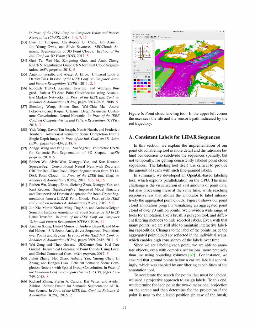
Figure 6: Point cloud labeling tool. In the upper left cornerthe user sees the tile and the sensor’s path indicated by thered trajectory.

A. Consistent Labels for LiDAR SequencesIn this section, we explain the implementation of our

point cloud labeling tool in more detail and the rationale be-hind our decision to subdivide the sequences spatially, butnot temporally, for getting consistently labeled point cloudsequences. The labeling tool itself was critical to providethe amount of scans with such fine-grained labels.

In summary, we developed an OpenGL-based labelingtool, which exploits parallelization on the GPU. The mainchallenge is the visualization of vast amounts of point data,but also processing these at the same time, while reachingresponsiveness that allows the annotator to label interac-tively the aggregated point clouds. Figure 6 shows our pointcloud annotation program visualizing an aggregated pointcloud of over 20 million points. We provide a wide range oftools for annotation, like a brush, a polygon tool, and differ-ent filtering methods to hide selected labels. Even with thatmany points, we are still able to maintain interactive label-ing capabilities. Changes to the label of the points inside theaggregated point cloud are reflected in the individual scans,which enables high consistency of the labels over time.

Since we are labeling each point, we are able to anno-tate objects, even with complex occlusions, more preciselythan just using bounding volumes [62]. For instance, weensured that ground points below a car are labeled accord-ingly, which was enabled by our filtering capabilities of theannotation tool.

To accelerate the search for points that must be labeled,we used a projective approach to assign labels. To this end,we determine for each point the two-dimensional projectionon the screen and then determine for the projection if thepoint is near to the clicked position (in case of the brush)

11

or inside the selected polygon. Therefore, annotators hadto ensure that they did not choose a view that essentiallydestroyed previously assigned points.

Usually, an annotator performed the following cycle toannotate points: (1) mark points with a specific label and (2)filter points with that label. Due to the filtering of alreadylabeled points, one can resolve occlusions and furthermoreensure that the aforementioned projective labeling does notdestroy already labeled points.

Tile-Based Labeling. An important detail is the afore-mentioned spatial subdivision of the complete aggregatedpoint cloud into tiles (also shown in the left upper part ofFigure 6). Initially, we simply rendered all scans in a rangeof timestamps, say 100 − 150, and then moved on the nextpart, say 150−200. However, this leads quickly to inconsis-tencies in the labels, since scans from such parts still overlapand therefore must be relabeled to match labels from be-fore. Since we, furthermore, encounter loop closures with aconsiderable temporal distance, this overlap can even hap-pen between parts of the sequences that are not temporallyclose, which even more complicated the task.

Thus, it quickly became apparent that such an additionaleffort to ensure consistent labels would lead to an unrea-sonable complicated annotations process and consequentlyto insufficient results. Therefore, we decided to subdividethe sequence spatially into tiles, where each tile contains allpoints from scans overlapping with this tile. Consistencyat the boundaries between tiles was achieved by having asmall overlap between the tiles, which enabled to consis-tently continue the labels from one tile into another neigh-boring tile.

Moving Objects. We annotated all moving objects, i.e.,car, truck, person, bicyclist, and motorcyclist, and eachmoving object is represented by a different class to distin-guish it from its corresponding non-moving class. In ourcase, we assigned an object the corresponding moving classwhen it moved at some point in time while observing it withthe sensor.

Since moving objects will appear at different placeswhen aggregating scans captured from different sensor lo-cations, we had to take special care to annotate moving ob-jects. This is especially challenging, when multiple types ofvehicles move on the same lane, like in most of the encoun-tered highway scenes. We annotated moving objects eitherby filtering ground points or by labeling each scan individ-ually, which was often necessary to label points of tires ofa car and bicycles or the feet of persons. But scan-by-scanlabeling was also necessary in aforementioned cases wheremultiple vehicles of different type drive on the same lane.The labeling of moving objects often was the first step whenannotating a tile, since this allowed the annotator to filter allmoving points and then concentrate on the static parts of theenvironment.

B. Basis of the DatasetThe basis of our dataset is data from the KITTI Vision

Benchmark [19], which is still the largest collection of dataalso used in autonomous driving at the time of writing. TheKITTI dataset is the basis of many experimental evaluationsin different contexts and was extended by novel tasks or ad-ditional data over time. Thus, we decided to build upon thislegacy and also enable synergies between our annotationsand other parts and tasks of the KITTI Vision Benchmark.

We particularly decided to use the Odometry Benchmarkto enable usage of the annotation data with this task. Weexpect that exploiting semantic information in the odome-try estimation is an interesting avenue for future research.However, also other tasks of the KITTI Vision Benchmarkmight profit from our annotations and the pre-trained mod-els we will publish on the dataset website.

Nevertheless, we hope that our effort and the availabilityof the point labeling tool will enable others to replicate ourwork on future publicly available datasets from an automo-tive LiDAR.

C. Class DefinitionIn the process of labeling such large amounts of data,

we had to decide which classes we want to be annotatedat some point in time. In general, we followed the classdefinitions and selection of the Mapillary Vistas dataset [39]and Cityscapes [10] dataset, but did some simplificationsand adjustments for the data source used.

First, we do not explicitly consider a rider class for per-sons riding a motorcycle or a bicycle, since the availablepoint clouds do not provide the density for a single scan todistinguish the person riding a vehicle. Furthermore, we getfor such classes only moving examples and therefore cannoteasily aggregate the point clouds to increase the fidelity ofthe point cloud and make it easier to distinguish the rider ofa vehicle and the vehicle.

The classes other-structure, other-vehicle, and other-object are fallback classes of their respective root categoryin unclear cases or missing classes, since this simplified thelabeling process and might be used to distinguish these cat-egories further in future.

Annotators often annotated some object or part of thescene and then hide the labeled points to avoid overwritingor removing the labels. Thus, assigning the fallback class inambiguous cases or cases where a specific class was missingmade it possible to simply hide that class to avoid overwrit-ing it. If we had instructed the annotators to label such partsas unlabeled, it would have caused problems to consistentlylabel the point clouds.

We furthermore distinguished between moving and non-moving vehicles and humans, i.e., a vehicle or human getsthe ‘moving’ tag if it moved in some consecutive scans

12

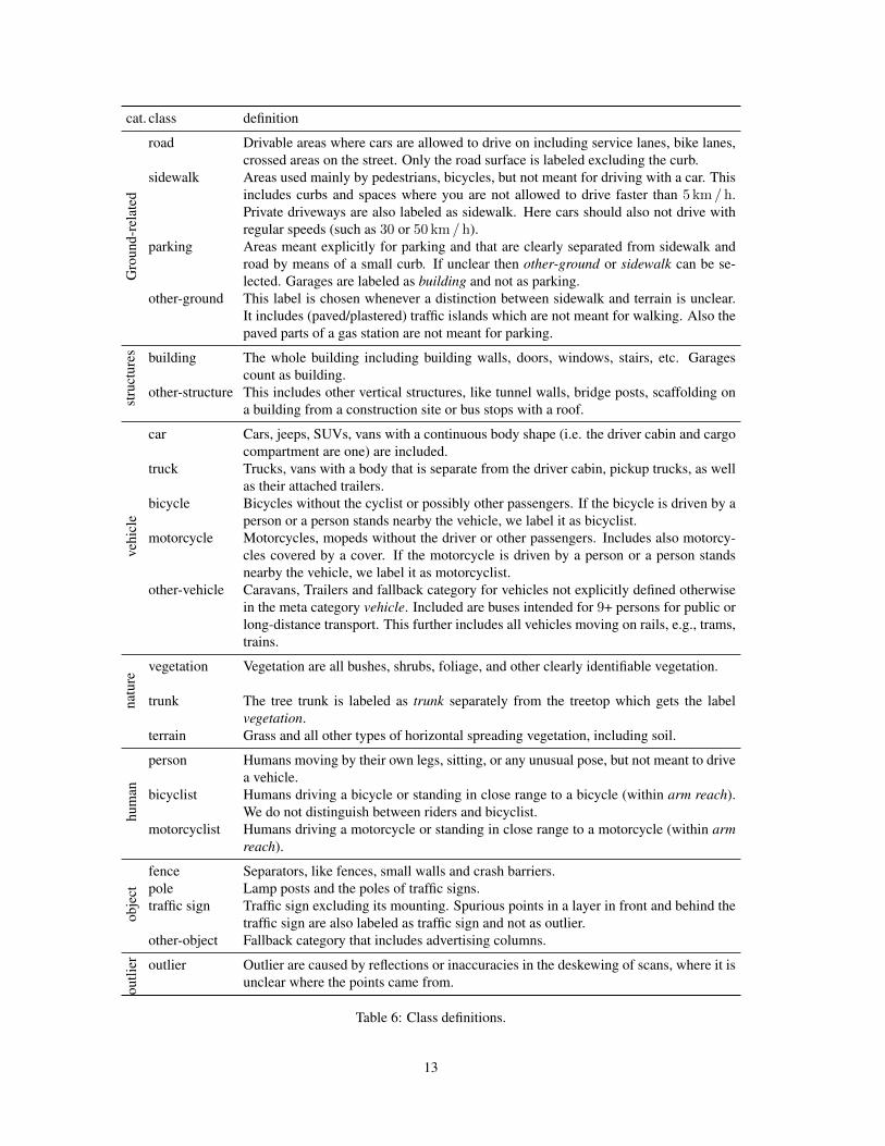
cat. class definitionG

roun

d-re

late

droad Drivable areas where cars are allowed to drive on including service lanes, bike lanes,

crossed areas on the street. Only the road surface is labeled excluding the curb.sidewalk Areas used mainly by pedestrians, bicycles, but not meant for driving with a car. This

includes curbs and spaces where you are not allowed to drive faster than 5 km / h.Private driveways are also labeled as sidewalk. Here cars should also not drive withregular speeds (such as 30 or 50 km / h).

parking Areas meant explicitly for parking and that are clearly separated from sidewalk androad by means of a small curb. If unclear then other-ground or sidewalk can be se-lected. Garages are labeled as building and not as parking.

other-ground This label is chosen whenever a distinction between sidewalk and terrain is unclear.It includes (paved/plastered) traffic islands which are not meant for walking. Also thepaved parts of a gas station are not meant for parking.

stru

ctur

es building The whole building including building walls, doors, windows, stairs, etc. Garagescount as building.

other-structure This includes other vertical structures, like tunnel walls, bridge posts, scaffolding ona building from a construction site or bus stops with a roof.

vehi

cle

car Cars, jeeps, SUVs, vans with a continuous body shape (i.e. the driver cabin and cargocompartment are one) are included.

truck Trucks, vans with a body that is separate from the driver cabin, pickup trucks, as wellas their attached trailers.

bicycle Bicycles without the cyclist or possibly other passengers. If the bicycle is driven by aperson or a person stands nearby the vehicle, we label it as bicyclist.

motorcycle Motorcycles, mopeds without the driver or other passengers. Includes also motorcy-cles covered by a cover. If the motorcycle is driven by a person or a person standsnearby the vehicle, we label it as motorcyclist.

other-vehicle Caravans, Trailers and fallback category for vehicles not explicitly defined otherwisein the meta category vehicle. Included are buses intended for 9+ persons for public orlong-distance transport. This further includes all vehicles moving on rails, e.g., trams,trains.

natu

re

vegetation Vegetation are all bushes, shrubs, foliage, and other clearly identifiable vegetation.

trunk The tree trunk is labeled as trunk separately from the treetop which gets the labelvegetation.

terrain Grass and all other types of horizontal spreading vegetation, including soil.

hum

an

person Humans moving by their own legs, sitting, or any unusual pose, but not meant to drivea vehicle.

bicyclist Humans driving a bicycle or standing in close range to a bicycle (within arm reach).We do not distinguish between riders and bicyclist.

motorcyclist Humans driving a motorcycle or standing in close range to a motorcycle (within armreach).

obje

ct

fence Separators, like fences, small walls and crash barriers.pole Lamp posts and the poles of traffic signs.traffic sign Traffic sign excluding its mounting. Spurious points in a layer in front and behind the

traffic sign are also labeled as traffic sign and not as outlier.other-object Fallback category that includes advertising columns.

outli

er outlier Outlier are caused by reflections or inaccuracies in the deskewing of scans, where it isunclear where the points came from.

Table 6: Class definitions.

13

Approach scan

size

proj

ecte

d

lear

ning

rate

epoc

hstr

aine

d

conv

erge

d

sing

lesc

an

PointNet 50 000 - 3 · 10−4×0.9epoch 33 3

PointNet++ 45 000 - 3 · 10−3×0.9epoch 25 3TangentConv 120 000 - 1 · 10−4 10 3SPLATNet 50 000 - 1 · 10−3 20 -SqueezeSeg 64× 2048 3 1 · 10−2×0.99epoch 200 3

DarkNet21Seg 64× 2048 3 1 · 10−3×0.99epoch 40 3

DarkNet53Seg 64× 2048 3 1 · 10−3×0.99epoch 120 3

mul

tisc

an TangentConv 500 000 - 5∗ 3

DarkNet53Seg64 64× 2048 3 1 · 10−3×0.99epoch 40∗ 3

Table 7: Approach statistics. ∗ in number of epochs meansthat it was started from the pretrained weights of the singlescan version.

while being observed by the LiDAR sensor.In summary, we annotated 28 classes and all annotated

classes with their respective definitions are listed in Table 6on the next page.

D. Baseline SetupWe modified the available implementations such that the

methods could be trained and evaluated on our large-scaledataset with very sparse point clouds due to the LiDAR sen-sor. Note that most of these approaches have so far onlybeen evaluated on small RGB-D indoor datasets.

We restricted the number of points within a single scandue to memory limitations on some approaches [40, 41] to50 000 via random sampling.

For SPLATNet, we used the SPLATNet3D1 architecturefrom [51]. The input consisted per point of the 3D posi-tion and its normal. The normals were previously estimatedgiven 30 closest neighbors.

With TangentConv2 we used the existing configurationfor Semantic3D. We sped up the training and validationprocedures by precomputing scan batches and added asyn-chronous data loading. Complete single scans were pro-vided during training. In the multi scan experiment we fixedthe number of points per batch to 500 000 due to mem-ory constraints and started training from the single scanweights.

For SqueezeSeg [60] and its Darknet backbone equiv-alents, we used a spherical projection of the scans in thesame way as the original SqueezeSeg approach. The pro-jection contains 64 lines in height corresponding with theseparate beams of the sensor, and extrapolating the config-uration of SqueezeSeg which only uses the front 90◦ anda horizontal resolution of 512, we use 2048 for the entirescan. Because some points are duplicated in this sampling

1https://github.com/NVlabs/splatnet2https://github.com/tatarchm/tangent_conv

process, we always keep the closest range value, and in in-ference of each scan we iterate over the entire point list andcheck it’s semantic value in the output grid.

An overview of the used parameters is given in Table 7.We furthermore provide the number of trained epochs andif we could get a results which seems to be converged in thegiven amount of time.

E. Results using Multiple Scans

The full per class IoU results for the multiple scans ex-periment are listed in Table 8. As already mentioned inthe main text, we generally observe that the IoU of staticclasses is mostly unaffected by the availability of multiplepast scans. To some extent, the IoU for some classes in-creases slightly. The drop in performance in terms of mIoUis mainly caused by the additional challenge to correctlyseparate moving and non-moving classes.

F. Semantic Scene Completion

Table 9 shows the class-wise results for semantic scenecompletion as well as precision and recall for scene com-pletion. One can see that TS3D + DarkNet53Seg performsslightly better than SSCNet and TS3D. Note that Dark-Net53Seg has been pretrained on the exact same classesas required for semantic scene completion. TS3D on theother hand uses DeepLab v2 (ResNet-101) [9] pretrainedon the Cityscapes [10] dataset, which does not differenti-ate between classes such as other-ground, parking or trunkfor example. Another reason might be that 2D semanticlabels projected back onto the point cloud is not very ac-curate especially at object boundaries, where labels oftenbleed onto distant objects. This is because in the 2D projec-tion, they are close to each other, a problem that is inherentto the projection method. The best approach (TS3D + Dark-Net53Seg + SATNet) outperforms the other approaches sig-nificantly (+20.77% IoU on scene completion and +7.51%mIoU on semantic scene completion). As mentioned above,it is the only approach capable of producing high resolutionoutputs. This approach however suffers from huge memoryconsumption. Therefore, during training the input volume israndomly cropped to volumes of grid size 64×64×32 whileduring inference, each volume gets divided into 6 overlap-ping blocks of size 90 × 138 × 32 for which the inferenceis performed individually. The individual blocks are subse-quently fused to obtain the final result. Figure 7 shows anexample result of this approach.

Rare classes like bicycle, motorcycle, motorcyclist, andperson are not or almost not recognized. This suggests thatthese classes are potentially hard to recognize, as they rep-resent a small and rare signal in the SemanticKITTI data.

14

Figure 7: Qualitative results for the semantic scene completion approach TS3D + DarkNet53Seg + SATNet. Left: Inputvolume. Middle: Network prediction. Right: Ground truth. Due to memory limitations the inference has to be done in sixsteps on overlapping subvolumes. The subvolumes are consequently fused to obtain the final result.

PointNet [40]

SPGraph [31]

SPLATNet [51]

PointNet++ [41]

SqueezeSeg [60]

TangentConv [52]

Darknet21Seg

Darknet53Seg

Ground truth

road sidewalk car

buildingterrainvegetation other-objecttrunk

parking pole

unlabeled

motorcycle

Figure 8: Examples of inference for all methods. The point clouds were projected to 2D using a spherical projection to makethe comparison easier.

15

Approach road

side

wal

k

park

ing

othe

r-gr

ound

build

ing

car

car(

mov

ing)

truc

k

truc

k(m

ovin

g)

bicy

cle

mot

orcy

cle

othe

r-ve

hicl

e

othe

r-ve

hicl

e(m

ovin

g)

vege

tatio

n

trun

k

terr

ain

pers

on

pers

on(m

ovin

g)

bicy

clis

t

bicy

clis

t(m

ovin

g)

mot

orcy

clis

t

mot

orcy

clis

t(m

ovin

g)

fenc

e

pole

traf

fic-s

ign

mIo

U

TangentConv 83.9 64.0 38.3 15.3 85.8 84.9 40.3 21.1 42.2 2.0 18.2 18.5 30.1 79.5 43.2 56.7 1.6 6.4 0.0 1.1 0.0 1.9 49.1 36.4 31.2 34.1DarkNet53Seg 91.6 75.3 64.9 27.5 85.2 84.1 61.5 20.0 37.8 30.4 32.9 20.7 28.9 78.4 50.7 64.8 7.5 15.2 0.0 14.1 0.0 0.2 56.5 38.1 53.3 41.6

Table 8: IoU results using a sequence of multiple past scans (in %).

Scene Completion Semantic Scene Completion

Approach prec

isio

n

reca

ll

IoU

road

side

wal

k

park

ing

othe

r-gr

ound

build

ing

car

truc

k

bicy

cle

mot

orcy

cle

othe

r-ve

hicl

e

vege

tatio

n

trun

k

terr

ain

pers

on

bicy

clis

t

mot

orcy

clis

t

fenc

e

pole

traf

ficsi

gn

mIo

U

SSCNet 31.71 83.40 29.83 27.55 16.99 15.60 6.04 20.88 10.35 1.79 0 0 0.11 25.77 11.88 18.16 0 0 0 14.40 7.90 3.67 9.53TS3D 31.58 84.18 29.81 28.00 16.98 15.65 4.86 23.19 10.72 2.39 0 0 0.19 24.73 12.46 18.32 0.03 0.05 0 13.23 6.98 3.52 9.54TS3D+ DarkNet53Seg 25.85 88.25 24.99 27.53 18.51 18.89 6.58 22.05 8.04 2.19 0.08 0.02 3.96 19.48 12.85 20.22 2.33 0.61 0.01 15.79 7.57 6.99 10.19TS3D+ DarkNet53Seg+ SATNet 80.52 57.65 50.60 62.20 31.57 23.29 6.46 34.12 30.70 4.85 0 0 0.07 40.12 21.88 33.09 0 0 0 24.05 16.89 6.94 17.70

Table 9: Results for scene completion and class-wise results for semantic scene completion (in %).

G. Qualitative ResultsFigure 8 shows qualitative results for the evaluated base-

line approaches on a scan from the validation data. Herewe show the spherical projections of the results to enablean easier comparison of the results.

With increasing performance in terms of mean IoU (topto bottom), see also Table 2 of the paper, we see that groundpoints get better separated into the classes sidewalk, road,and parking. In particular, parking areas need a lot of con-textual information and also information from neighboringpoints, since often a small curb distinguishes the parkingarea from the road.

In general, one can see definitely an increased accuracyfor smaller objects like the poles on the right side of the im-age, which indicates that the extra parameters of the modelswith the largest capacity (25 million as in the case of Dark-Net21Seg and 50 million as in the case of Darknet53Seg)are needed to distinguish smaller classes and class with fewexamples.

H. Dataset and Baseline Access APIAlong with the annotations and the labeling tool, we also

provide a public API implemented in Python.In contrast to our labeling tool, which is intended for al-

lowing users to easily extend this dataset, and generate oth-ers for other purposes, this API is intended to be used to eas-ily access the data, calculate statistics, evaluate metrics, andaccess several implementations of different state-of-the-art

semantic segmentation approaches. We hope that this APIwill serve as a baseline to implement new point cloud se-mantic segmentation approaches, and will provide a com-mon framework to evaluate them, and compare them moretransparently with other methods. The choice of Python asthe underlying language for the API is that it is the cur-rent language of choice for the front end for deep learn-ing framework developers, and therefore, for deep learningpractitioners.

Figure 9 gives an overview of the labeled sequencesshowing the estimated trajectories and the aggregated pointcloud over the whole sequence.

16

00 01 02 03 04

05 06 07 08

09 10 11 12

13 14 15 16 17

18 19 20 21

Figure 9: Qualitative overview of labeled sequences and trajectories.

17