Semantic Structure from Motion

Sid Yingze Bao and Silvio SavareseDepartment of Electrical and Computer Engineering, University of Michigan at Ann Arbor

{yingze,silvio}@eecs.umich.edu

Abstract

Conventional rigid structure from motion (SFM) ad-dresses the problem of recovering the camera parameters(motion) and the 3D locations (structure) of scene points,given observed 2D image feature points. In this paper, wepropose a new formulation called Semantic Structure FromMotion (SSFM). In addition to the geometrical constraintsprovided by SFM, SSFM takes advantage of both seman-tic and geometrical properties associated with objects inthe scene (Fig. 1). These properties allow us to recovernot only the structure and motion but also the 3D loca-tions, poses, and categories of objects in the scene. Wecast this problem as a max-likelihood problem where ge-ometry (cameras, points, objects) and semantic information(object classes) are simultaneously estimated. The key intu-ition is that, in addition to image features, the measurementsof objects across views provide additional geometrical con-straints that relate cameras and scene parameters. Theseconstraints make the geometry estimation process more ro-bust and, in turn, make object detection more accurate.Our framework has the unique ability to: i) estimate cam-era poses only from object detections, ii) enhance camerapose estimation, compared to feature-point-based SFM al-gorithms, iii) improve object detections given multiple un-calibrated images, compared to independently detecting ob-jects in single images. Extensive quantitative results onthree datasets – LiDAR cars, street-view pedestrians, andKinect office desktop – verify our theoretical claims.

1. IntroductionUnderstanding the 3D spatial and semantic structure of

complex scenes from images is one of the critical capa-bilities of an intelligent visual system. Consider the pho-tographs in Fig. 1(a). These show the same environmentobserved from a handful of viewpoints. Even if this isthe first time you (the observer) have seen this environ-ment, it is not difficult to infer: i) the spatial structure ofthe scene and the way objects are organized in the physi-cal space; ii) the semantic content of the scene and its in-dividual components. State-of-the-art methods for objectrecognition [9, 20, 10, 19] typically describe the scene with

image

(a)

chair desk

monitor

chair

desk

monitor

chair

cameracamera

desk

monitor

monitor

(b)

(c) (d)

cameracamera

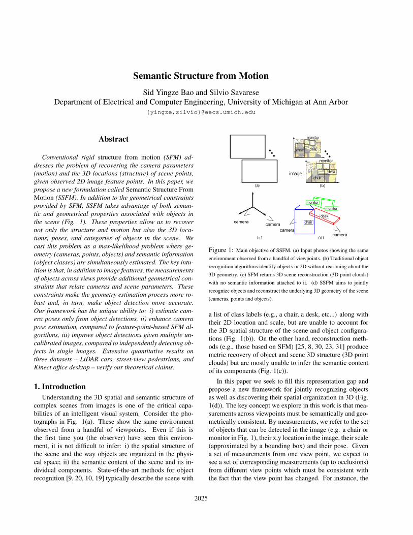
Figure 1: Main objective of SSFM. (a) Input photos showing the sameenvironment observed from a handful of viewpoints. (b) Traditional objectrecognition algorithms identify objects in 2D without reasoning about the3D geometry. (c) SFM returns 3D scene reconstruction (3D point clouds)with no semantic information attached to it. (d) SSFM aims to jointlyrecognize objects and reconstruct the underlying 3D geometry of the scene(cameras, points and objects).

a list of class labels (e.g., a chair, a desk, etc...) along withtheir 2D location and scale, but are unable to account forthe 3D spatial structure of the scene and object configura-tions (Fig. 1(b)). On the other hand, reconstruction meth-ods (e.g., those based on SFM) [25, 8, 30, 23, 31] producemetric recovery of object and scene 3D structure (3D pointclouds) but are mostly unable to infer the semantic contentof its components (Fig. 1(c)).

In this paper we seek to fill this representation gap andpropose a new framework for jointly recognizing objectsas well as discovering their spatial organization in 3D (Fig.1(d)). The key concept we explore in this work is that mea-surements across viewpoints must be semantically and geo-metrically consistent. By measurements, we refer to the setof objects that can be detected in the image (e.g. a chair ormonitor in Fig. 1), their x,y location in the image, their scale(approximated by a bounding box) and their pose. Givena set of measurements from one view point, we expect tosee a set of corresponding measurements (up to occlusions)from different view points which must be consistent withthe fact that the view point has changed. For instance, the

2025

chair in Fig. 1(a) appears in two views and its location,scale and pose variation across the two views must be con-sistent with the view point transformation. In this work weexploit this property and introduce a novel joint probabilitymodel where object detection and 3D structure estimationare solved in a coherent fashion.

Our proposed method has the merit of enhancing both3D reconstruction and visual recognition capabilities in twoways: i) Enhancing 3D reconstruction: Our framework canhelp overcome a crucial limitation of scene/object modelingmethods. State-of-the-art SFM techniques mostly fail whendealing with challenging camera configurations (e.g., whenthe views are too few and the view baseline is too large).This failure occurs as it is very hard to establish correct fea-ture correspondences for widely separated views. For in-stance, the 3D reconstruction in Fig. 1(c) was obtained us-ing a state-of-the-art SFM algorithm [13] using 43 densely-sampled pictures of an office. The same algorithm wouldnot work if we just used the two images in Fig. 1(a) forthe reasons mentioned above. By reasoning at the seman-tic level, and by establishing object correspondences acrossviews, our framework creates the conditions for overcomingthis limitation. We show that our framework has the abil-ity to estimate camera poses from object detections only.Moreover, our framework can still exploit traditional SFMconstraints based on feature correspondences to make the3D reconstruction process robust. We show that our methodcan significantly outperform across-view feature matchingSFM algorithms such as [30, 22] (Tab. 1). ii) Enhancing vi-sual recognition: Traditional recognition methods are typi-cally prone to produce false alarms when appearance cuesare not discriminative enough and no contextual informa-tion about the scene is available. For instance, the cabinetin Fig. 1(a) can be easily confused with a monitor as theyboth share similar appearance characteristics. By reasoningat the geometrical level, our framework is able to identifythose hypotheses that are not consistent with the underly-ing geometry and reduce their confidence score accordingly.Our model leads to promising experimental results showingimprovements in object detection rates compared with thestate-of-the-art methods such as [9] (Fig. 4 and Tab. 2).Also, we show that we can automatically establish objectcorrespondence across views.

Recently, a number of approaches have explored theidea of combining semantic cues with geometrical con-straints for scene understanding. Notable examples are[14, 29, 21, 32, 16]. These focus on single images and,unlike our work, they do not attempt to enforce consis-tency across views. Moreover, they make restrictive as-sumptions on the camera and scene configuration. Othermethods have been proposed to track objects with multi-view geometry [18], but they assume that the underlyingscene geometry is available. A large number of works have

proposed solutions for interpreting complex scenes from 3Ddata [11, 17, 27, 26] or a combination of 3D data and im-agery [3]. However, in most of these methods 3D informa-tion is either provided by external devices (e.g. 3D scanningsystems such as LiDAR) or using traditional SFM tech-niques. In either case, unlike our framework, the recogni-tion and reconstruction steps are separated and independent.[5] attempts joint estimation using a “cognitive loop” butrequires a dedicated stereo-camera architecture and makesassumptions about camera motion. To our best knowledge,this is the first work that seeks to make these two steps co-herent within a setting that requires only images with un-calibrated cameras (up to internal parameters) and arbitraryscene-camera configurations.2. The Semantic Structure from Motion Model

Conventional rigid structure from motion (SFM) ad-dresses the problem of recovering camera parameters C andthe 3D locations of scene points Q, given observed 2D im-age feature points. In this paper, we propose a new for-mulation where, in addition to the geometrical constraintsprovided by SFM, we take advantage of both the seman-tic and geometrical properties associated with objects in thescene in order to recover C and Q as well as the 3D loca-tions, poses, and category memberships of objects O in thescene. We call this semantic structure from motion (SSFM).The key intuition is that, in addition to image features, themeasurements of objects across views provides additionalgeometrical constraints that relate camera and scene param-eters. We formulate SSFM as a maximum likelihood esti-mation (MLE) problem whose goal is to find the best con-figuration of cameras, 3D points and 3D objects that arecompatible with the measurements provided by a set of im-ages.2.1. Problem Formulation

In this section we define the SSFM problem and formu-late it as an MLE problem. We first define the main vari-ables involved in SSFM, and then discuss the MLE formu-lation.

Cameras. Let C denote the camera parameters. C ={Ck} = {Kk, Rk, T k} where K is the camera matrix cap-turing the internal parameters, R rotation matrix, and Ttranslation vector with respect to a common world refer-ence system. K is assumed to be known, whereas {R, T}are unknown. Throughout this paper, the camera is indexedby k as a superscript.

3D Points Q and Measurements q,u. Let Q = {Qs}denote a set of 3D points Qs. Each 3D point Qs is speci-fied by (Xs, Ys, Zs) describing the 3D point location in theworld reference system. Q is an unknown in our problem.Denote by q = {qki } the set of point measurements (imagefeatures) for all the cameras. Namely, qki is the ith pointmeasurement in image (camera) k. A point measurementis described by the measurement vector qk = {x, y, a}ki ,

2026

camera

Image Plane

wh

x,y

Θ

Φ

n

tq

r

rs

X,Y,Z

φ

θ

n

t

q

Z

YX

w

ww(a) (b)

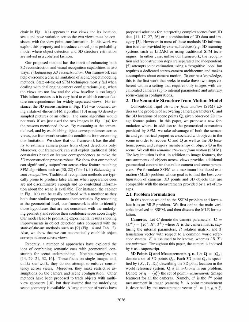
Figure 2: 3D object’s location and pose parametrization. (a) Assume anobject is enclosed by the tightest possible bounding cube. The object 3Dlocation X,Y, Z is the centroid of the bounding cube. The object’s poseis defined by the bounding cube’s three perpendicular surface’s norms thatare n, q, t and parametrized by the angles Θ,Φ in a given world referencesystem (b). r is the ray connecting O and the camera center. Let zenithangle φ be the angle between r and n, and azimuth angle θ be the anglebetween q and rS , where rS is the projection of r onto the plane perpen-dicular to n. We parametrize an object measurement in the image by thelocation x, y of tightest bounding box enclosing the object, the width wand height h of the bounding box (object 2D scale), the object pose θ, φ,and class c.

where x, y describe the point image location, and a is a lo-cal descriptor that captures the local neighborhood appear-ance of the point in image k. These measurements maybe obtained using feature detectors and descriptors such as[22, 34]. Since each image measurement {qki } is assumedto correspond to a certain physical 3D point Qs, we modelsuch correspondence by introducing an indicator variableuki , where uki = s if {qki } corresponds to Qs. A similarnotation was also introduced in [7]. A set of indicator vari-ables u = {uki } allows us to establish feature correspon-dences across views and to relate feature matches with 3Dpoint candidates (Sec. 2.3). Unlike [7], we assume the fea-ture correspondences can be measured by feature matchingalgorithms such as [22]. Throughout this paper, Q and qare indexed by s and i respectively and they appear as sub-scripts.

3D Objects O and Measurements o. Let O = {Ot}denote a set of 3D objects Ot. The tth 3D objects Ot isspecified by a 3D location (Xt, Yt, Zt), a pose (Θt,Φt),and a category label ct (e.g, car, person, etc...). Thus, a3D object is parametrized byOt = (X,Y, Z,Θ,Φ, c)t (Fig.2). The set O is an unknown in our problem. Denote byo = {okj } the set of object measurements for all the cam-eras. Thus, okj is the jth measurement of an object in image(camera) k. An object measurement is described by the fol-lowing measurement vector okj = {x, y, w, h, θ, φ, c}kj (Fig.2). As discussed in Sec. 2.2, these measurements may beobtained using any state-of-the art object detector that canreturn the probability that certain location x, y in an imageis occupied by an object with category c, scale h,w, andpose θ, φ (e.g. [28]) 1. Similar to the 3D point case, sinceeach object measurement {okj } from image k is assumed tocorrespond to some physical 3D object Ot, such correspon-dence may be modeled by introducing an indicator variable

1State of the art object detectors such as [9] can be modified so as toenable pose classification, as discussed in Sec.4.1.

vkj , where vkj = t if okj corresponds to 3D object Ot. How-ever, for the object case, we seek to estimate object cor-respondence automatically as part of our inference process(Sec. 3). Thus, from this point on, we assume 3D objectobservations are given by o. We denote 3D object and 2Dobject using the subscript index t and j respectively.

MLE formulation. Our goal is to estimate a configura-tion of Q, O and C that is consistent with the feature pointmeasurements q,u and the object measurements o. We for-mulate this estimation as the one of finding Q,O,C suchthat the joint likelihood is maximized:

{Q,O,C} = arg maxQ,O,C

Pr(q,u,o|Q,O,C)

= arg maxQ,O,C

Pr(q,u|Q,C) Pr(o|O,C) (1)

where the last expression is obtained by assuming that,given C, Q and O, the measurements associated with 3Dobjects and 3D points are conditionally independent. In thenext two sections we show how to estimate the two like-lihood terms Pr(q,u|Q,C) (Eq. 4 or 5) and Pr(o|O,C)(Eq. 3).2.2. Object Likelihood Pr(o|O,C)

Pr(o|O,C) measures the likelihood of object measure-ments o given the the camera and object configurationsO,C. This term can be estimated by computing the agree-ment between predicted measurements and actual measure-ments. Predicted measurements are obtained by introducinga mapping ωkt = ωk(Ot) = ωk((X,Y, Z,Θ,Φ, c)t) that re-lates the parameters describing the 3D object Ot to the im-age of camera Ck. Thus, ωkt is a parameter vector that con-tains the predicted location, pose, scale and category of Otin Ck. Next, we present expressions for predicting the mea-surements and relating them to actual measurements and forobtaining an estimate of the likelihood term.

Computing Predicted Measurements. The transfor-mation ωkt = ωk(Ot) can be computed once cameras C areknown. Specifically, let us denote by Xk

t , Ykt , Z

kt the 3D

location of Ot in the reference system of Ck and by Θkt ,Φ

kt

its 3D pose (these can be obtained from Xt, Yt, Zt,Θt,Φtin the world reference system by means of a (known)rigid transformation). Predicted location (xkt , y

kt ) and pose

(φkt , θkt ) of Ot in camera Ck can be computed by us-

ing the camera projection matrix [15] as [xkt , ykt , 1]′ =

Kk[Xkt , Y

kt , Z

kt ]′/Zkt and [φkt , θ

kt ] = [Φkt ,Θ

kt ]. Predicting

2D object scales in the image requires a more complex geo-metrical derivation that goes beyond the scope of this paper.We introduce an approximated simplified mapping definedas follows:{

wkt = fk ·W (Θkt ,Φ

kt , ct)/Z

kt

hkt = fk ·H(Θkt ,Φ

kt , ct)/Z

kt

(2)

where wkt , hkt denote the predicted object 2D scale (sim-

ilar to Fig. 2), fk is the focal length of the kth cam-era. W (Θk

t ,Φkt , ct) or H(Θk

t ,Φkt , ct) is a (scalar) mapping

that describes the typical relationship between physical ob-

2027

Detector Scale

Large

Small

Detector PoseInput Image

Apply Detector

...

...

M=15

Lx

Ly

(x,y)Tensor

Representation

1 2 3 4 5

1

2

3

Detection Probability Tensor

DetectionProbability

Maps

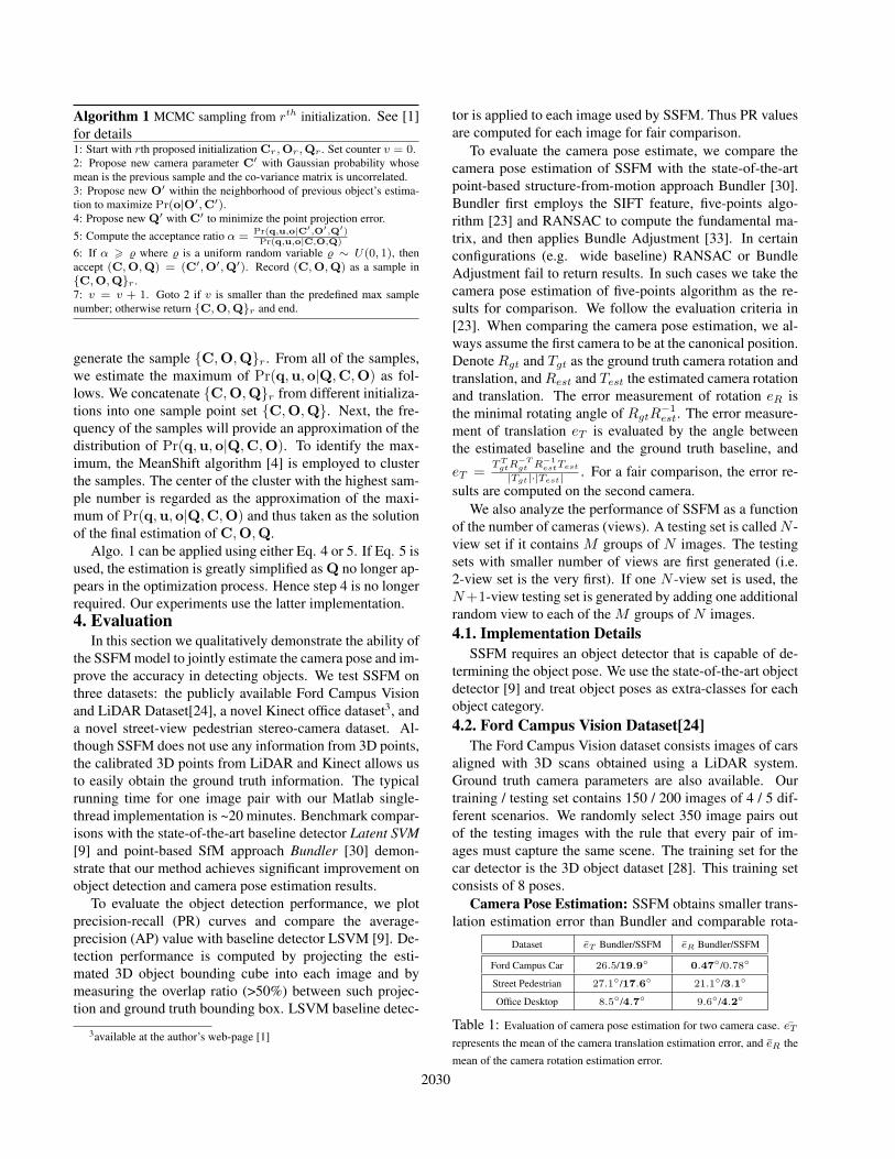
Figure 3: Multi-pose and multi-scale object detection illustration. The “probability maps” are obtained by applying car detector with different scales andposes on the left image. The color from red to deep blue indicates the detector response from high to low. We used LSVM [9] (Sec. 4.1) to obtain theseprobability maps. In this example, Ξ has dimensions Lx × Ly × 15. If the scale=3 (small), pose=4, and category=car, Π will return the index π = 14 (thered circle). Thus, Ξ(x, y, 14) will return the confidence of detecting a car at small scale and pose=4 at location x, y in the image (the orange rectangle).

ject bounding cube and object image bounding box. Thismapping is a function of the object pose Θk

t ,Φkt and cat-

egory ct. It can be learned by using ground truth 3D ob-ject bounding cubes and corresponding observations usingML regressor [1]. In conclusion, the equations above al-low us to fully estimate the object prediction vector ωkt ={x, y, w, h, φ, θ, c}kt for object Ot in camera Ck.

Measurements as Probability Maps. Pr(o|O,C) canbe now estimated by computing the agreement between pre-dicted measurements and actual measurements. Such agree-ment is readily available using the set of probability valuesreturned by object detectors such as [9] applied to images(Fig. 3). The output of this detection process for the im-age of Ck is a tensor Ξk of M probability maps whereineach map captures the likelihood that an object of categoryc with scale w, h and pose θ, φ presents at location x, y inthe image. Thus, we can interpret Ξk as one Lx × Ly ×Mtensor, where Lx and Ly are the image width and height andM adds up to the number of object categories, scales andposes. Let us denote by Π : {w, h, φ, θ, c} → π ∈ 1 . . .Mthe indexing function that allows retrieval from Ξk the de-tection probability at any location x, y given a set of valuesfor scale, pose and category. Fig. 3 shows an example ofa set of 15 probability maps for only one object category(i.e., the car category), three scales and five poses associ-ated with a given image. Notice that since measurementscan be extracted directly from Ξk once the mapping 3D-object-image ω is computed, the 2D objects of the kth im-age are automatically associated with the 3D objects. Asa result, across-view one-to-one object correspondences arealso established.

Estimating the likelihood term. The key idea is thatthe set Ξk of probability maps along with π can be usedto estimate Pr(o|O,C) given the predicted measurements.To illustrate this, let us start by considering an estima-tion of the likelihood term Pr(o|Ot, Ck) for Ot observedfrom camera Ck. Using ωkt , we can predict the object’sscale {w, h}kt , pose {φ, θ}kt and category ckt . This al-lows us to retrieve from Ξk the probability of detecting anobject at the predicted location {x, y}kt by using the in-dexing function πkt , and in turn estimate Pr(o|Ot, Ck) =Ξk(xkt , y

kt , π(wkt , h

kt , φ

kt , θ

kt , c

kt )). Assuming that objects

are independent from each other and camera configurationsare independent, the joint likelihood of objects and camerascan be approximated as:

Pr(o|O,C) ∝Nt∏t

Pr(o|Ot,C) ∝Nt∏t

(1−Nk∏k

(1− Pr(o|Ot, Ck)))

(3)where Nt is the number of objects and Nk is the number ofcameras. Nt is in general unknown, but it can be estimatedusing detection probability maps (Sec.3.1). Notice that thisterm does not penalize objects that are observed only by aportion of images while they are truncated or occluded inother images. Pr(o|Ot,C) is only partially affected by anoccluded or truncated object Ot in the kth image even if theobject leads to a low value for Pr(o|Ot, Ck).2.3. Points Likelihood Pr(q,u|Q,C)

Pr(q,u|Q,C) measures the likelihood of the 3D pointsand cameras given the measurements of 3D points and theircorrespondences across views. This likelihood term can beestimated by computing the agreement between predictedmeasurements and actual measurements. Similar to the 3Dobject case, predicted measurements are obtained by intro-ducing a mapping from 3D points to the images.

Predicted Measurements. Predicted measurements canbe easily obtained once the cameras C are known. We in-dicate by qks the predicted measurement of the sth point Qsin camera Ck which can be computed by using the cameraCk projection matrix, similar to Sec. 2.2. Recall that qksis expressing a location x, y in pixels in the image. Sincewe know which point is being projected, we have a predic-tion for the indicator variable as well. This is equivalentto predicting the projection qks of Qs to camera Ck and theprojection qks of Qs to Ck are in correspondence.

Point Measurements. Point measurements are denotedby qki = {x, y, a}ki , where x, y describe the point locationin image k of measurement i, and a is a local descriptor thatcaptures the local appearance of the point in a neighbor-hood of image k. We obtain location measurements {x, y}kiusing a DOG detector equipped with a SIFT descriptor forestimating aki [22]. Measurements for feature correspon-dences (matches) across images are obtained by matchingthe point features.

Estimating the likelihood term. Pr(q,u|Q,C) canbe estimated by computing the agreement between pre-dicted measurements and the actual measurements. To il-lustrate this, let us start by considering the likelihood termPr(q|Os, Ck) for one point Qs and for camera Ck. As in-troduced in [7], one possible strategy for computing such

2028

agreement assumes that the location of measurements andpredictions are equal up to a noise n - that is, qki = qks + n,where s = uki . If we assume zero mean Gaussian noise,we can estimate Pr(qki |Qs, Ck) ∝ exp(−(qki − qkuki )2/σq),leading to the following expression for the likelihood:

Pr(q,u|Q,C) =

NQ∏i

Nk∏k

exp(−(qki − qkuki )2/σq) (4)

where Nk is the number of cameras, NQ is the number ofpoints, and σq is the variance of 2D point projection mea-surement error. This is obtained by assuming independenceamong points and among cameras.

We also propose an alternative estimator forPr(q,u|Q,C). While this estimator leads to a coarserapproximation for the likelihood, it makes the inferenceprocess more efficient and produces more stable results.This new estimator exploits the epipolar constraints relatingcamera pairs. Given a pair of cameras Cl and Ck, wecan estimate the fundamental matrix Fl,k. Suppose qki ,qlj are from Ck and Cl respectively, and the matchingalgorithm predicts that qki and qlj are in correspondence.Fl,k can predict the epipolar line ξl,ki (or ξk,lj ) of qki (orqlj) in image Cl (or Ck). If we model the distance2 dl,kj,ibetween ξl,ki and qlj as zero-mean Gaussian with varianceσu, Pr(qki , q

lj |Qs, Cl, Ck) ∝ exp(−dl,kj,i/σu). Notice that

this expression does not account for appearance similaritybetween matched features – that is the similarity betweenthe descriptors aki and alj . We model appearance similarity

as exp(−α(aki ,alj)

σα) where α(·, ·) captures the distance

between two feature vectors and σα the variance of theappearance similarity. Overall, we obtain the followingexpression for the likelihood term:

Pr(q,u|Q,C) ∝Nk∏k 6=l

Ns∏i 6=j

Pr(qki , qlj |Qs, Cl, Ck)

∝Nk∏k 6=l

Ns∏i 6=j

exp(−dl,kj,i

σu) exp(−

α(aki , alj)

σα) (5)

Eq. 5 is obtained by assuming that feature locations and ap-pearance are independent. During the learning stage, welearn the variance σu and σα using an ML estimator ona validation set. Notice that Pr(q,u|Q,C) is no longer afunction of Qs. This significantly reduces the search spacefor solving the MLE problem.3. Max-Likelihood Estimation with Sampling

Our goal is to estimate camera parameters, points, andobjects so as to maximize Eq. 1. Due to the high dimension-ality of the parameter space, we propose to sample C,Q,Ofrom Pr(q,u,o|Q,C,O) similar to [7]. This allows usto approximate the distribution of Pr(q,u,o|Q,C,O) and

2To account for outliers, we set a threshold on dl,kj,i . Namely, if dl,kj,iis the measurement, we set dl,kj,i = min(dl,kj,i ,Γ). We learn the outlierthreshold Γ using a validation set.

find the C,Q,O that maximize the likelihood. In Sec. 3.1we discuss the initialization of the sampling process, and inSec. 3.2 we describe a modified formulation of the MarkovChain Monte Carlo (MCMC) sampling algorithm for solv-ing the MLE problem.3.1. Parameter Initialization

Appropriate initialization of cameras, objects, and pointsis a critical step in the sampling method. We initialize cam-era configurations (i.e. estimate camera configurations thatare geometrically compatible with the observations) usingfeature point matches and object detections.

Camera Initialization by Feature Points. We follow[23] to initialize (estimate) C from image measurements q.Due to the metric reconstruction ambiguity, we scale theestimated camera translation with several random values toobtain several camera pose initializations.

Camera Initialization by Objects. We use a standardobject detector [9] to detect 2D objects and estimate objectpose and scale (Sec. 4.1). Next, we use such object detec-tions to form possible object correspondences and use theseto estimate several possible initial camera configurations.It can be shown [1] that object pose and scale consistencyconstraints (across views) can be used to reduce the largenumber of possible initial configurations.

Points and Objects Initialization. Camera configura-tions obtained by using points and objects form the initial-ization set. For each of these configurations, object detec-tions are used to initialize objects in 3D using the map-ping in Eq. 2. If certain initialized 3D objects are toonear to others (location and pose-wise), they are mergedto a single one. Similarly, for each camera configura-tion, feature points q are used to initialize 3D points Q bytriangulation[15]. Correspondences between q and Q areestablished after the initialization. We use index r to indi-cate one out of R possible initializations for objects, cam-eras and points (Cr,Or,Qr).3.2. Sample and Maximize the Likelihood

We sample C,O,Q from the underlyingPr(q,u,o|Q,C,O) using a modified Metropolis al-gorithm [12] (Algo. 1). Since the goal of the sampling isto identify a maximum, the samples should occur as nearto max Pr(q,u,o|Q,C,O) as possible, so as to increasethe efficiency of the sampling algorithm. Thus, we onlyrandomly sample C, while the best configuration of Oand Q given the proposed C are estimated during eachsampling step. In step 3, the estimation of O′ is obtainedby greedy search within a neighborhood of the objectsproposed during the previous sampling step. Since theobject detection scale and pose are highly quantized, thegreedy search yields efficient and robust results in practice.The estimation of Q is based on the minimization of theprojection error (similar to [33]).

Following Algo. 1 and using the rth initialization, we

2029

Algorithm 1 MCMC sampling from rth initialization. See [1]for details1: Start with rth proposed initialization Cr,Or,Qr . Set counter v = 0.2: Propose new camera parameter C′ with Gaussian probability whosemean is the previous sample and the co-variance matrix is uncorrelated.3: Propose new O′ within the neighborhood of previous object’s estima-tion to maximize Pr(o|O′,C′).4: Propose new Q′ with C′ to minimize the point projection error.

5: Compute the acceptance ratio α =Pr(q,u,o|C′,O′,Q′)Pr(q,u,o|C,O,Q)

6: If α > % where % is a uniform random variable % ∼ U(0, 1), thenaccept (C,O,Q) = (C′,O′,Q′). Record (C,O,Q) as a sample in{C,O,Q}r .7: v = v + 1. Goto 2 if v is smaller than the predefined max samplenumber; otherwise return {C,O,Q}r and end.

generate the sample {C,O,Q}r. From all of the samples,we estimate the maximum of Pr(q,u,o|Q,C,O) as fol-lows. We concatenate {C,O,Q}r from different initializa-tions into one sample point set {C,O,Q}. Next, the fre-quency of the samples will provide an approximation of thedistribution of Pr(q,u,o|Q,C,O). To identify the max-imum, the MeanShift algorithm [4] is employed to clusterthe samples. The center of the cluster with the highest sam-ple number is regarded as the approximation of the maxi-mum of Pr(q,u,o|Q,C,O) and thus taken as the solutionof the final estimation of C,O,Q.

Algo. 1 can be applied using either Eq. 4 or 5. If Eq. 5 isused, the estimation is greatly simplified as Q no longer ap-pears in the optimization process. Hence step 4 is no longerrequired. Our experiments use the latter implementation.4. Evaluation

In this section we qualitatively demonstrate the ability ofthe SSFM model to jointly estimate the camera pose and im-prove the accuracy in detecting objects. We test SSFM onthree datasets: the publicly available Ford Campus Visionand LiDAR Dataset[24], a novel Kinect office dataset3, anda novel street-view pedestrian stereo-camera dataset. Al-though SSFM does not use any information from 3D points,the calibrated 3D points from LiDAR and Kinect allows usto easily obtain the ground truth information. The typicalrunning time for one image pair with our Matlab single-thread implementation is ~20 minutes. Benchmark compar-isons with the state-of-the-art baseline detector Latent SVM[9] and point-based SfM approach Bundler [30] demon-strate that our method achieves significant improvement onobject detection and camera pose estimation results.

To evaluate the object detection performance, we plotprecision-recall (PR) curves and compare the average-precision (AP) value with baseline detector LSVM [9]. De-tection performance is computed by projecting the esti-mated 3D object bounding cube into each image and bymeasuring the overlap ratio (>50%) between such projec-tion and ground truth bounding box. LSVM baseline detec-

3available at the author’s web-page [1]

tor is applied to each image used by SSFM. Thus PR valuesare computed for each image for fair comparison.

To evaluate the camera pose estimate, we compare thecamera pose estimation of SSFM with the state-of-the-artpoint-based structure-from-motion approach Bundler [30].Bundler first employs the SIFT feature, five-points algo-rithm [23] and RANSAC to compute the fundamental ma-trix, and then applies Bundle Adjustment [33]. In certainconfigurations (e.g. wide baseline) RANSAC or BundleAdjustment fail to return results. In such cases we take thecamera pose estimation of five-points algorithm as the re-sults for comparison. We follow the evaluation criteria in[23]. When comparing the camera pose estimation, we al-ways assume the first camera to be at the canonical position.Denote Rgt and Tgt as the ground truth camera rotation andtranslation, andRest and Test the estimated camera rotationand translation. The error measurement of rotation eR isthe minimal rotating angle of RgtR−1

est. The error measure-ment of translation eT is evaluated by the angle betweenthe estimated baseline and the ground truth baseline, and

eT =TTgtR

−Tgt R

−1estTest

|Tgt|·|Test| . For a fair comparison, the error re-sults are computed on the second camera.

We also analyze the performance of SSFM as a functionof the number of cameras (views). A testing set is calledN -view set if it contains M groups of N images. The testingsets with smaller number of views are first generated (i.e.2-view set is the very first). If one N -view set is used, theN+1-view testing set is generated by adding one additionalrandom view to each of the M groups of N images.4.1. Implementation Details

SSFM requires an object detector that is capable of de-termining the object pose. We use the state-of-the-art objectdetector [9] and treat object poses as extra-classes for eachobject category.4.2. Ford Campus Vision Dataset[24]

The Ford Campus Vision dataset consists images of carsaligned with 3D scans obtained using a LiDAR system.Ground truth camera parameters are also available. Ourtraining / testing set contains 150 / 200 images of 4 / 5 dif-ferent scenarios. We randomly select 350 image pairs outof the testing images with the rule that every pair of im-ages must capture the same scene. The training set for thecar detector is the 3D object dataset [28]. This training setconsists of 8 poses.

Camera Pose Estimation: SSFM obtains smaller trans-lation estimation error than Bundler and comparable rota-

Dataset eT Bundler/SSFM eR Bundler/SSFM

Ford Campus Car 26.5/19.9◦ 0.47◦/0.78◦

Street Pedestrian 27.1◦/17.6◦ 21.1◦/3.1◦

Office Desktop 8.5◦/4.7◦ 9.6◦/4.2◦

Table 1: Evaluation of camera pose estimation for two camera case. eTrepresents the mean of the camera translation estimation error, and eR themean of the camera rotation estimation error.

2030

SSFM Cali. Cam.

SSFM uncali. cam.

Latent SVM

AP=62.1%

AP=61.3%

AP=54.5% Recall

Precision

(a) Car

Recall

Precision

SSFM Cali. Cam.

SSFM Uncali. Cam.

Latent SVM

AP=75.1%

AP=74.2%

AP=70.1%

(b) Pedestrian

SSFM Cali. Cam.

SSFM uncali. cam.

Latent SVM

AP=52.1%

AP=51.6%

AP=49.0%

Precision

Recall

(c) Office

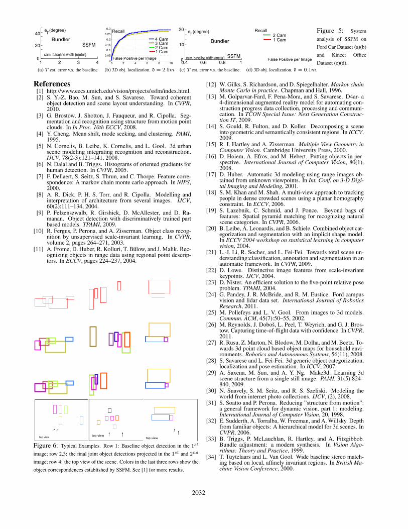
Figure 4: Detection PR results by SSFM with cali-brated cameras (green), SSFM with uncalibrated cam-eras (blue) and LSVM [9] (red). Fig. 4c shows av-erage results for mouse, keyboard and monitor cate-gories. SSFM is applied on image pairs randomly se-lected from the testing set (unless otherwise stated).Calibration is obtained from ground truth.

tion estimation error (Tab. 1).Object Detection: The PR by SSFM and the baseline

detector are plotted in Fig. 4a. Since ground truth anno-tation for small objects is difficult to obtain accurately, inthis dataset we only test scales whose bounding box areasare larger than 0.6% of the image area. SSFM improves thedetection precision and recall.

Camera Baseline Width v.s. Pose Estimation: We an-alyze the effect of baseline width on the camera pose esti-mation. Since the rotation estimations of both Bundler andSSFM contain little error, we only show the translation es-timation error v.s. camera baseline width (Fig. 5a). Thisexperiment confirms the intuition that a wider baseline im-pacts more dramatically the performance of methods basedon low level feature matching than does on methods such asSSFM where higher level semantics are used.

Comparison for Different Number of Cameras: Tab.2 shows the camera pose estimation error and the objectdetection AP as a function of the number of views (cameras)used to run SSFM. As more cameras are available, SSFMtends to achieve better object detection result and cameratranslation estimation.

3D Object Localization Performance: Due to themetric-reconstruction ambiguity, we use calibrated camerasin this experiment to enforce that the coordinates of 3D ob-jects have a physical meaning. We manually label the 3Dbounding boxes of cars on the LiDAR 3D point cloud toobtain the ground truth car 3D locations. We consider a 3Ddetection to be true positive if the distance between its cen-troid and ground truth 3D object centroid is smaller than athreshold d (see figure captions). The 3D object localizationfor one camera (single view) is obtained by using its 2Dbounding box scale and location [2]. SSFM performanceincreases as the number of views grows (Fig. 5b).

Object-based Structure from Motion: We disable thefeature point detection and matching, thus no 2D points areused (i.e. just maximize Pr(o|C,O)). For the two-viewcase, the detection AP increases from the baseline 54.5% to55.2%, while the error of camera pose estimation is eT =81.2◦ and eR = 21.2◦. To the best of our knowledge, this isthe first time SFM has been tested based only on high-level

Camera # 2 3 4

Det. AP (Cali. Cam.) 62.1% 63.6% 64.2%

Det. AP (Uncali. Cam.) 61.3% 61.7% 62.6%

eT 19.9◦ 16.2◦ 13.9◦

Table 2: Camera pose estimation errors and object detection AP v.s.numbers of cameras on the Ford-car dataset. The baseline detector AP is54.5%.

cues (objects) rather than low-level / middle-level cues (e.g.points, lines, or areas).4.3. Kinect Office Desktop Dataset[1]

We use Microsoft’s Kinect to collect images and corre-sponding 3D range data of several static indoor office envi-ronments. The ground truth camera parameters are obtainedby aligning range data across different views. We manuallyidentify the locations of ground truth 3D object boundingcubes similarly to the way we process Ford dataset. The ob-jects in this dataset are monitors, keyboards, and mice. Thetesting and training sets contain 5 different office desktopscenarios respectively and each scenario has ~50 images.From each scenario, we randomly select 100 image pairs fortesting or training. SSFM performance is evaluated usingthe ground truth information and compared against baselinealgorithms. We show these results as Fig. 4c, Tab. 1, Fig.5c, and Fig. 5d. Refer to the figure captions for more de-tails.4.4. Stereo Street-view Pedestrian Dataset

We collected this dataset by simultaneously capturingpairs of images of street-view pedestrians. The two camerasare pre-calibrated so that the ground-truth camera poses aremeasured and known. The object category in this datasetis pedestrian. The training set of object detector is INRIApedestrian dataset [6] with no pose label. The two cam-eras are parallel and their relative distance is 4m. The typ-ical object-to-camera distance is 5 ∼ 10m. The trainingset contains 200 image pairs in 5 different scenarios. Thetesting set contains 200 image pairs in 6 other scenarios.SSFM attains smaller camera pose estimation error com-pared to Bundler (Tab. 1) and better detection rates thanLSVM (Fig. 4b). Notice in this dataset the baseline widthof the two cameras is fixed thus we cannot analyze the cam-era pose estimation error v.s. camera baseline width andcannot carry out experiments with multiple cameras.5. Conclusion

This paper presents a new paradigm called the semanticstructure from motion for jointly estimating 3D objects, 3Dpoints and camera poses from multiple images. We see thiswork as a promising step toward the goal of coherently in-terpreting the geometrical and semantic content of complexscenes.Acknowledgments

We acknowledge the support of NSF CAREER#1054127 and the Gigascale Systems Research Center. Wewish to thank Mohit Bagra for his help in collecting theKinect dataset and Min Sun for helpful feedback.

2031

1 2 3 40

20

40

SSFMBundler

e (degree)T

cam. baseline width (meter)

(a) T est. error v.s. the baseline

0 2 4 6 8 100

0.05

0.1

0.15

0.2

0.25

0.3Recall

False Positive per Image

3 Cam2 Cam1 Cam

4 Cam

(b) 3D obj. localization. d = 2.5m

0.4 0.6 0.8 10

10

20

SSFM

Bundler

e (degree)T

cam. baseline width (meter)

(c) T est. error v.s. the baseline.

2 Cam1 Cam

Recall

False Positive per Image

(d) 3D obj. localization. d = 0.1m.

Figure 5: Systemanalysis of SSFM onFord Car Dataset (a)(b)and Kinect OfficeDataset (c)(d).

References[1] http://www.eecs.umich.edu/vision/projects/ssfm/index.html.[2] S. Y.-Z. Bao, M. Sun, and S. Savarese. Toward coherent

object detection and scene layout understanding. In CVPR,2010.

[3] G. Brostow, J. Shotton, J. Fauqueur, and R. Cipolla. Seg-mentation and recognition using structure from motion pointclouds. In In Proc. 10th ECCV, 2008.

[4] Y. Cheng. Mean shift, mode seeking, and clustering. PAMI,1995.

[5] N. Cornelis, B. Leibe, K. Cornelis, and L. Gool. 3d urbanscene modeling integrating recognition and reconstruction.IJCV, 78(2-3):121–141, 2008.

[6] N. Dalal and B. Triggs. Histograms of oriented gradients forhuman detection. In CVPR, 2005.

[7] F. Dellaert, S. Seitz, S. Thrun, and C. Thorpe. Feature corre-spondence: A markov chain monte carlo approach. In NIPS,2000.

[8] A. R. Dick, P. H. S. Torr, and R. Cipolla. Modelling andinterpretation of architecture from several images. IJCV,60(2):111–134, 2004.

[9] P. Felzenszwalb, R. Girshick, D. McAllester, and D. Ra-manan. Object detection with discriminatively trained partbased models. TPAMI, 2009.

[10] R. Fergus, P. Perona, and A. Zisserman. Object class recog-nition by unsupervised scale-invariant learning. In CVPR,volume 2, pages 264–271, 2003.

[11] A. Frome, D. Huber, R. Kolluri, T. Bülow, and J. Malik. Rec-ognizing objects in range data using regional point descrip-tors. In ECCV, pages 224–237, 2004.

top view top viewtop view

Figure 6: Typical Examples. Row 1: Baseline object detection in the 1st

image; row 2,3: the final joint object detections projected in the 1st and 2nd

image; row 4: the top view of the scene. Colors in the last three rows show theobject correspondences established by SSFM. See [1] for more results.

[12] W. Gilks, S. Richardson, and D. Spiegelhalter. Markov chainMonte Carlo in practice. Chapman and Hall, 1996.

[13] M. Golparvar-Fard, F. Pena-Mora, and S. Savarese. D4ar- a4-dimensional augmented reality model for automating con-struction progress data collection, processing and communi-cation. In TCON Special Issue: Next Generation Construc-tion IT, 2009.

[14] S. Gould, R. Fulton, and D. Koller. Decomposing a sceneinto geometric and semantically consistent regions. In ICCV,2009.

[15] R. I. Hartley and A. Zisserman. Multiple View Geometry inComputer Vision. Cambridge University Press, 2000.

[16] D. Hoiem, A. Efros, and M. Hebert. Putting objects in per-spective. International Journal of Computer Vision, 80(1),2008.

[17] D. Huber. Automatic 3d modeling using range images ob-tained from unknown viewpoints. In Int. Conf. on 3-D Digi-tal Imaging and Modeling, 2001.

[18] S. M. Khan and M. Shah. A multi-view approach to trackingpeople in dense crowded scenes using a planar homographyconstraint. In ECCV, 2006.

[19] S. Lazebnik, C. Schmid, and J. Ponce. Beyond bags offeatures: Spatial pyramid matching for recognizing naturalscene categories. In CVPR, 2006.

[20] B. Leibe, A. Leonardis, and B. Schiele. Combined object cat-egorization and segmentation with an implicit shape model.In ECCV 2004 workshop on statistical learning in computervision, 2004.

[21] L.-J. Li, R. Socher, and L. Fei-Fei. Towards total scene un-derstanding:classification, annotation and segmentation in anautomatic framework. In CVPR, 2009.

[22] D. Lowe. Distinctive image features from scale-invariantkeypoints. IJCV, 2004.

[23] D. Nister. An efficient solution to the five-point relative poseproblem. TPAMI, 2004.

[24] G. Pandey, J. R. McBride, and R. M. Eustice. Ford campusvision and lidar data set. International Journal of RoboticsResearch, 2011.

[25] M. Pollefeys and L. V. Gool. From images to 3d models.Commun. ACM, 45(7):50–55, 2002.

[26] M. Reynolds, J. Doboš, L. Peel, T. Weyrich, and G. J. Bros-tow. Capturing time-of-flight data with confidence. In CVPR,2011.

[27] R. Rusu, Z. Marton, N. Blodow, M. Dolha, and M. Beetz. To-wards 3d point cloud based object maps for household envi-ronments. Robotics and Autonomous Systems, 56(11), 2008.

[28] S. Savarese and L. Fei-Fei. 3d generic object categorization,localization and pose estimation. In ICCV, 2007.

[29] A. Saxena, M. Sun, and A. Y. Ng. Make3d: Learning 3dscene structure from a single still image. PAMI, 31(5):824–840, 2009.

[30] N. Snavely, S. M. Seitz, and R. S. Szeliski. Modeling theworld from internet photo collections. IJCV, (2), 2008.

[31] S. Soatto and P. Perona. Reducing ”structure from motion”:a general framework for dynamic vision. part 1: modeling.International Journal of Computer Vision, 20, 1998.

[32] E. Sudderth, A. Torralba, W. Freeman, and A. Willsky. Depthfrom familiar objects: A hierarchical model for 3d scenes. InCVPR, 2006.

[33] B. Triggs, P. McLauchlan, R. Hartley, and A. Fitzgibbob.Bundle adjustment: a modern synthesis. In Vision Algo-rithms: Theory and Practice, 1999.

[34] T. Tuytelaars and L. Van Gool. Wide baseline stereo match-ing based on local, affinely invariant regions. In British Ma-chine Vision Conference, 2000.

2032