Semantic Image Inpainting with Deep Generative Models

Raymond A. Yeh∗, Chen Chen∗, Teck Yian Lim,Alexander G. Schwing, Mark Hasegawa-Johnson, Minh N. Do

University of Illinois at Urbana-Champaign{yeh17, cchen156, tlim11, aschwing, jhasegaw, minhdo}@illinois.edu

Abstract

Semantic image inpainting is a challenging task wherelarge missing regions have to be filled based on the avail-able visual data. Existing methods which extract informa-tion from only a single image generally produce unsatisfac-tory results due to the lack of high level context. In this pa-per, we propose a novel method for semantic image inpaint-ing, which generates the missing content by conditioningon the available data. Given a trained generative model,we search for the closest encoding of the corrupted imagein the latent image manifold using our context and priorlosses. This encoding is then passed through the generativemodel to infer the missing content. In our method, infer-ence is possible irrespective of how the missing content isstructured, while the state-of-the-art learning based methodrequires specific information about the holes in the trainingphase. Experiments on three datasets show that our methodsuccessfully predicts information in large missing regionsand achieves pixel-level photorealism, significantly outper-forming the state-of-the-art methods.

1. Introduction

Semantic inpainting [30] refers to the task of inferring ar-bitrary large missing regions in images based on image se-mantics. Since prediction of high-level context is required,this task is significantly more difficult than classical inpaint-ing or image completion which is often more concernedwith correcting spurious data corruption or removing entireobjects. Numerous applications such as restoration of dam-aged paintings or image editing [3] benefit from accuratesemantic inpainting methods if large regions are missing.However, inpainting becomes increasingly more difficult iflarge regions are missing or if scenes are complex.

Classical inpainting methods are often based on eitherlocal or non-local information to recover the image. Mostexisting methods are designed for single image inpainting.

∗Authors contributed equally.

Input TV LR PM Ours

Figure 1. Semantic inpainting results by TV, LR, PM and ourmethod. Holes are marked by black color.

Hence they are based on the information available in theinput image, and exploit image priors to address the ill-posed-ness. For example, total variation (TV) based ap-proaches [34, 1] take into account the smoothness propertyof natural images, which is useful to fill small missing re-gions or remove spurious noise. Holes in textured imagescan be filled by finding a similar texture from the same im-age [6]. Prior knowledge, such as statistics of patch off-sets [11], planarity [13] or low rank (LR) [12] can greatlyimprove the result as well. PatchMatch (PM) [2] searchesfor similar patches in the available part of the image andquickly became one of the most successful inpainting meth-ods due to its high quality and efficiency. However, all sin-gle image inpainting methods require appropriate informa-tion to be contained in the input image, e.g., similar pixels,structures, or patches. This assumption is hard to satisfy, ifthe missing region is large and possibly of arbitrary shape.Consequently, in this case, these methods are unable to re-cover the missing information. Fig. 1 shows some chal-lenging examples with large missing regions, where local

1

arX

iv:1

607.

0753

9v3

[cs

.CV

] 1

3 Ju

l 201

7

methods fail to recover the nose and eyes.In order to address inpainting in the case of large missing

regions, non-local methods try to predict the missing pixelsusing external data. Hays and Efros [10] proposed to cutand paste a semantically similar patch from a huge database.Internet based retrieval can be used to replace a target regionof a scene [37]. Both methods require exact matching fromthe database or Internet, and fail easily when the test sceneis significantly different from any database image. Unlikeprevious hand-crafted matching and editing, learning basedmethods have shown promising results [27, 38, 33, 22]. Af-ter an image dictionary or a neural network is learned, thetraining set is no longer required for inference. Oftentimes,these learning-based methods are designed for small holesor for removing small text in the image.

Instead of filling small holes in the image, we are inter-ested in the more difficult task of semantic inpainting [30].It aims to predict the detailed content of a large region basedon the context of surrounding pixels. A seminal approachfor semantic inpainting, and closest to our work is the Con-text Encoder (CE) by Pathak et al. [30]. Given a maskindicating missing regions, a neural network is trained toencode the context information and predict the unavailablecontent. However, the CE only takes advantage of the struc-ture of holes during training but not during inference. Henceit results in blurry or unrealistic images especially whenmissing regions have arbitrary shapes.

In this paper, we propose a novel method for seman-tic image inpainting. We consider semantic inpainting asa constrained image generation problem and take advan-tage of the recent advances in generative modeling. Aftera deep generative model, i.e., in our case an adversarial net-work [9, 32], is trained, we search for an encoding of thecorrupted image that is “closest” to the image in the latentspace. The encoding is then used to reconstruct the imageusing the generator. We define “closest” by a weighted con-text loss to condition on the corrupted image, and a priorloss to penalizes unrealistic images. Compared to the CE,one of the major advantages of our method is that it doesnot require the masks for training and can be applied forarbitrarily structured missing regions during inference. Weevaluate our method on three datasets: CelebA [23], SVHN[29] and Stanford Cars [17], with different forms of missingregions. Results demonstrate that on challenging semanticinpainting tasks our method can obtain much more realisticimages than the state of the art techniques.

2. Related WorkA large body of literature exists for image inpainting, and

due to space limitations we are unable to discuss all of it indetail. Seminal work in that direction includes the afore-mentioned works and references therein. Since our methodis based on generative models and deep neural nets, we will

Figure 2. Images generated by a VAE and a DCGAN. First row:samples from a VAE. Second row: samples from a DCGAN.

review the technically related learning based work in thefollowing.Generative Adversarial Networks (GANs) are a frame-work for training generative parametric models, and havebeen shown to produce high quality images [9, 4, 32]. Thisframework trains two networks, a generator, G, and a dis-criminator D. G maps a random vector z, sampled from aprior distribution pZ, to the image space while D maps aninput image to a likelihood. The purpose ofG is to generaterealistic images, while D plays an adversarial role, discrim-inating between the image generated from G, and the realimage sampled from the data distribution pdata.

TheG andD networks are trained by optimizing the lossfunction:

minG

maxD

V (G,D) =Eh∼pdata(h)[log(D(h))]+

Ez∼pZ(z)[log(1−D(G(z))], (1)

where h is the sample from the pdata distribution; z is arandom encoding on the latent space.

With some user interaction, GANs have been applied ininteractive image editing [40]. However, GANs can not bedirectly applied to the inpainting task, because they producean entirely unrelated image with high probability, unlessconstrained by the provided corrupted image.Autoencoders and Variational Autoencoders (VAEs) [16]have become a popular approach to learning of complexdistributions in an unsupervised setting. A variety of VAEflavors exist, e.g., extensions to attribute-based image edit-ing tasks [39]. Compared to GANs, VAEs tend to generateoverly smooth images, which is not preferred for inpaintingtasks. Fig. 2 shows some examples generated by a VAE anda Deep Convolutional GAN (DCGAN) [32]. Note that theDCGAN generates much sharper images. Jointly trainingVAEs with an adveserial loss prevents the smoothness [18],but may lead to artifacts.

The Context Encoder (CE) [30] can be also viewed as anautoencoder conditioned on the corrupted images.

It produces impressive reconstruction results when thestructure of holes is fixed during both training and infer-ence, e.g., fixed in the center, but is less effective for arbi-trarily structured regions.

2

G DReal or

Fake

𝐺(𝒛(0)) 𝐺(𝒛(1)) 𝐺(ො𝒛)Input Blending

−𝜕𝐿𝑝𝜕𝒛

−𝜕𝐿𝑐𝜕𝒛

𝐺(𝒛)

𝒚 𝐌

𝐿𝑜𝑠𝑠 = 𝐿𝑝 𝒛 + 𝐿𝑐 𝒛 , )

𝒛

(a) (b)

Figure 3. The proposed framework for inpainting. (a) Given a GAN model trained on real images, we iteratively update z to find the closestmapping on the latent image manifold, based on the desinged loss functions. (b) Manifold traversing when iteratively updating z usingback-propagation. z(0) is random initialed; z(k) denotes the result in k-th iteration; and z denotes the final solution.

Back-propagation to the input data is employed in ourapproach to find the encoding which is close to the providedbut corrupted image. In earlier work, back-propagationto augment data has been used for texture synthesis andstyle transfer [8, 7, 20]. Google’s DeepDream uses back-propagation to create dreamlike images [28]. Additionally,back-propagation has also been used to visualize and un-derstand the learned features in a trained network, by “in-verting” the network through updating the gradient at theinput layer [26, 5, 35, 21]. Similar to our method, allthese back-propagation based methods require specificallydesigned loss functions for the particular tasks.

3. Semantic Inpainting by Constrained ImageGeneration

To fill large missing regions in images, our method forimage inpainting utilizes the generator G and the discrimi-nator D, both of which are trained with uncorrupted data.After training, the generator G is able to take a point zdrawn from pZ and generate an image mimicking samplesfrom pdata. We hypothesize that if G is efficient in its rep-resentation then an image that is not from pdata (e.g., cor-rupted data) should not lie on the learned encoding mani-fold, z. Therefore, we aim to recover the encoding z “clos-est” to the corrupted image while being constrained to themanifold, as illustrated in Fig. 3; we visualize the latentmanifold, using t-SNE [25] on the 2-dimensional space, andthe intermediate results in the optimization steps of findingz. After z is obtained, we can generate the missing contentby using the trained generative model G.

More specifically, we formulate the process of finding zas an optimization problem. Let y be the corrupted imageand M be the binary mask with size equal to the image,to indicate the missing parts. An example of y and M isshown in Fig. 3 (a).

Using this notation we define the “closest” encoding zvia:

z = argminz{Lc(z|y,M) + Lp(z)}, (2)

where Lc denotes the context loss, which constrains thegenerated image given the input corrupted image y and thehole mask M; Lp denotes the prior loss, which penalizesunrealistic images. The details of the proposed loss func-tion will be discussed in the following sections.

Besides the proposed method, one may also consider us-ing D to update y by maximizing D(y), similar to back-propagation in DeepDream [28] or neural style transfer [8].However, the corrupted data y is neither drawn from areal image distribution nor the generated image distribution.Therefore, maximizing D(y) may lead to a solution that isfar away from the latent image manifold, which may hencelead to results with poor quality.

3.1. Importance Weighted Context Loss

To fill large missing regions, our method takes advantageof the remaining available data. We designed the contextloss to capture such information. A convenient choice forthe context loss is simply the `2 norm between the gener-ated sample G(z) and the uncorrupted portion of the inputimage y. However, such a loss treats each pixel equally,which is not desired. Consider the case where the center

3

block is missing: a large portion of the loss will be frompixel locations that are far away from the hole, such as thebackground behind the face. Therefore, in order to find thecorrect encoding, we should pay significantly more atten-tion to the missing region that is close to the hole.

To achieve this goal, we propose a context loss with thehypothesis that the importance of an uncorrupted pixel ispositively correlated with the number of corrupted pixelssurrounding it. A pixel that is very far away from any holesplays very little role in the inpainting process. We capturethis intuition with the importance weighting term, W,

Wi =

∑

j∈N(i)

(1−Mj)|N(i)| if Mi 6= 0

0 if Mi = 0, (3)

where i is the pixel index, Wi denotes the importanceweight at pixel location i, N(i) refers to the set of neigh-bors of pixel i in a local window, and |N(i)| denotes thecardinality of N(i). We use a window size of 7 in all exper-iments.

Empirically, we also found the `1-norm to performslightly better than the `2-norm in our framework. Taking itall together, we define the conextual loss to be a weighted`1-norm difference between the recovered image and theuncorrupted portion, defined as follows,

Lc(z|y,M) = ‖W � (G(z)− y)‖1. (4)

Here, � denotes the element-wise multiplication.

3.2. Prior Loss

The prior loss refers to a class of penalties based onhigh-level image feature representations instead of pixel-wise differences. In this work, the prior loss encourages therecovered image to be similar to the samples drawn fromthe training set. Our prior loss is different from the onedefined in [14] which uses features from pre-trained neuralnetworks.

Our prior loss penalizes unrealistic images. Recall thatin GANs, the discriminator, D, is trained to differentiategenerated images from real images. Therefore, we choosethe prior loss to be identical to the GAN loss for training thediscriminator D, i.e.,

Lp(z) = λ log(1−D(G(z))). (5)

Here, λ is a parameter to balance between the two losses. zis updated to fool D and make the corresponding generatedimage more realistic. Without Lp, the mapping from y toz may converge to a perceptually implausible result. Weillustrate this by showing the unstable examples where weoptimized with and without Lp in Fig. 4.

Real Input Ours w/o Lp Ours w Lp

Figure 4. Inpainting with and without the prior loss.

3.3. Inpainting

With the defined prior and context losses at hand, thecorrupted image can be mapped to the closest z in the latentrepresentation space, which we denote z. z is randomlyinitialized and updated using back-propagation on the totalloss given in Eq. (2). Fig. 3 (b) shows for one example thatz is approaching the desired solution on the latent imagemanifold.

After generating G(z), the inpainting result can be eas-ily obtained by overlaying the uncorrupted pixels from theinput. However, we found that the predicted pixels may notexactly preserve the same intensities of the surrounding pix-els, although the content is correct and well aligned. Pois-son blending [31] is used to reconstruct our final results.The key idea is to keep the gradients of G(z) to preserveimage details while shifting the color to match the color inthe input image y. Our final solution, x, can be obtainedby:

x = argminx‖∇x−∇G(z)‖22,

s.t. xi = yi for Mi = 1, (6)

where ∇ is the gradient operator. The minimization prob-lem contains a quadratic term, which has a unique solution[31]. Fig. 5 shows two examples where we can find visibleseams without blending.

Overlay Blend Overlay Blend

Figure 5. Inpainting with and without blending.

3.4. Implementation Details

In general, our contribution is orthogonal to specificGAN architectures and our method can take advantage ofany generative model G. We used the DCGAN model ar-chitecture from Radford et al. [32] in the experiments. The

4

generative model, G, takes a random 100 dimensional vec-tor drawn from a uniform distribution between [−1, 1] andgenerates a 64×64×3 image. The discriminator model,D,is structured essentially in reverse order. The input layer isan image of dimension 64× 64× 3, followed by a series ofconvolution layers where the image dimension is half, andthe number of channels is double the size of the previouslayer, and the output layer is a two class softmax.

For training the DCGAN model, we follow the trainingprocedure in [32] and use Adam [15] for optimization. Wechoose λ = 0.003 in all our experiments. We also per-form data augmentation of random horizontal flipping onthe training images. In the inpainting stage, we need to findz in the latent space using back-propagation. We use Adamfor optimization and restrict z to [−1, 1] in each iteration,which we observe to produce more stable results. We ter-minate the back-propagation after 1500 iterations. We usethe identical setting for all testing datasets and masks.

4. ExperimentsIn the following section we evaluate results qualitatively

and quantitatively, more comparisons are provided in thesupplementary material.

4.1. Datasets and Masks

We evaluate our method on three dataset: the CelebFacesAttributes Dataset (CelebA) [23], the Street View HouseNumbers (SVHN) [29] and the Stanford Cars Dataset [17].

The CelebA contains 202, 599 face images with coarsealignment [23]. We remove approximately 2000 imagesfrom the dataset for testing. The images are cropped at thecenter to 64 × 64, which contain faces with various view-points and expressions.

The SVHN dataset contains a total of 99,289 RGB im-ages of cropped house numbers. The images are resized to64 × 64 to fit the DCGAN model architecture. We usedthe provided training and testing split. The numbers in theimages are not aligned and have different backgrounds.

The Stanford Cars dataset contains 16,185 images of 196classes of cars. Similar as the CelebA dataset, we do not useany attributes or labels for both training and testing. Thecars are cropped based on the provided bounding boxes andresized to 64× 64. As before, we use the provided trainingand test set partition.

We test four different shapes of masks: 1) central blockmasks; 2) random pattern masks [30] in Fig. 1, with ap-proximately 25% missing; 3) 80% missing complete ran-dom masks; 4) half missing masks (randomly horizontal orvertical).

4.2. Visual Comparisons

Comparisons with TV and LR inpainting. We compareour method with local inpainting methods. As we already

Input TV LR OursReal

Figure 6. Comparisons with local inpainting methods TV and LRinpainting on examples with random 80% missing.

Real Input Ours NN

Figure 7. Comparisons with nearest patch retrieval.

showed in Fig. 1, local methods generally fail for largemissing regions. We compare our method with TV inpaint-ing [1] and LR inpainting [24, 12] on images with small ran-dom holes. The test images and results are shown in Fig. 6.Due to a large number of missing points, TV and LR basedmethods cannot recover enough image details, resulting invery blurry and noisy images. PM [2] cannot be applied tothis case due to insufficient available patches.Comparisons with NN inpainting. Next we compare ourmethod with nearest neighbor (NN) filling from the trainingdataset, which is a key component in retrieval based meth-ods [10, 37]. Examples are shown in Fig. 7, where the mis-alignment of skin texture, eyebrows, eyes and hair can beclearly observed by using the nearest patches in Euclideandistance. Although people can use different features for re-trieval, the inherit misalignment problem cannot be easilysolved [30]. Instead, our results are obtained automaticallywithout any registration.Comparisons with CE. In the remainder, we compare our

5

Table 1. The PSNR values (dB) on the test sets. Left/right resultsare by CE[30]/ours.

Masks/Dataset CelebA SVHN CarsCenter 21.3/19.4 22.3/19.0 14.1/13.5pattern 19.2/17.4 22.3/19.8 14.0/14.1random 20.6/22.8 24.1/33.0 16.1/18.9

half 15.5/13.7 19.1/14.6 12.6/11.1

result with those obtained from the CE [30], the state-of-the-art method for semantic inpainting. It is important tonote that the masks is required to train the CE. For a faircomparison, we use all the test masks in the training phasefor the CE. However, there are infinite shapes and missingratios for the inpainting task. To achieve satisfactory resultsone may need to re-train the CE. In contrast, our method canbe applied to arbitrary masks without re-training the net-work, which is according to our opinion a huge advantagewhen considering inpainting applications.

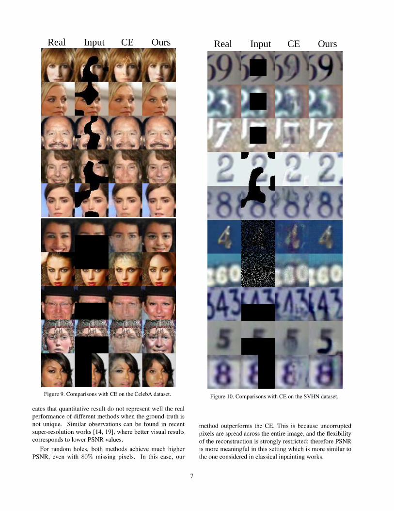
Figs. 8 and 9 show the results on the CelebA dataset withfour types of masks. Despite some small artifacts, the CEperforms best with central masks. This is due to the fact thatthe hole is always fixed during both training and testing inthis case, and the CE can easily learn to fill the hole from thecontext. However, random missing data, is much more dif-ficult for the CE to learn. In addition, the CE does not usethe mask for inference but pre-fill the hole with the meancolor. It may mistakenly treat some uncorrupted pixels withsimilar color as unknown. We could observe that the CE hasmore artifacts and blurry results when the hole is at randompositions. In many cases, our results are as realistic as thereal images. Results on SVHN and car datasets are shownin Figs. 10 and 11, and our method generally produces vi-sually more appealing results than the CE since the imagesare sharper and contain fewer artifacts.

4.3. Quantitative Comparisons

It is important to note that semantic inpainting is not try-ing to reconstruct the ground-truth image. The goal is to fillthe hole with realistic content. Even the ground-truth im-age is one of many possibilities. However, readers may beinterested in quantitative results, often reported by classicalinpainting approaches. Following previous work, we com-pare the PSNR values of our results and those by the CE.The real images from the dataset are used as groundtruthreference. Table 1 provides the results on the three datasets.The CE has higher PSNR values in most cases except forthe random masks, as they are trained to minimize the meansquare error. Similar results are obtained using SSIM [36]instead of PSNR. These results conflict with the aforemen-tioned visual comparisons, where our results generally yieldto better perceptual quality.

We investigate this claim by carefully investigating theerrors of the results. Fig. 12 shows the results of one exam-

Real Input CE Ours

Figure 8. Comparisons with CE on the CelebA dataset.

ple and the corresponding error images. Judging from thefigure, our result looks artifact-free and very realistic, whilethe result obtained from the CE has visible artifacts in thereconstructed region. However, the PSNR value of CE is1.73dB higher than ours. The error image shows that ourresult has large errors in hair area, because we generate ahairstyle which is different from the real image. This indi-

6

Real Input CE Ours

Figure 9. Comparisons with CE on the CelebA dataset.

cates that quantitative result do not represent well the realperformance of different methods when the ground-truth isnot unique. Similar observations can be found in recentsuper-resolution works [14, 19], where better visual resultscorresponds to lower PSNR values.

For random holes, both methods achieve much higherPSNR, even with 80% missing pixels. In this case, our

Real Input CE Ours

Figure 10. Comparisons with CE on the SVHN dataset.

method outperforms the CE. This is because uncorruptedpixels are spread across the entire image, and the flexibilityof the reconstruction is strongly restricted; therefore PSNRis more meaningful in this setting which is more similar tothe one considered in classical inpainting works.

7

Real Input CE Ours

Figure 11. Comparisons with CE on the car dataset.

4.4. Discussion

While the results are promising, the limitation of ourmethod is also obvious. Indeed, its prediction performancestrongly relies on the generative model and the training pro-cedure. Some failure examples are shown in Fig. 13, whereour method cannot find the correct z in the latent image

Input CE Ours

Real CE Error × 2 Ours Error × 2

Figure 12. The error images for one example. The PSNR for con-text encoder and ours are 24.71 dB and 22.98 dB, respectively.The errors are amplified for display purpose.

Ours

Input

Real

Figure 13. Some failure examples.

manifold. The current GAN model in this paper workswell for relatively simple structures like faces, but is toosmall to represent complex scenes in the world. Conve-niently, stronger generative models, improve our method ina straight-forward way.

5. ConclusionIn this paper, we proposed a novel method for semantic

inpainting. Compared to existing methods based on localimage priors or patches, the proposed method learns the rep-resentation of training data, and can therefore predict mean-ingful content for corrupted images. Compared to CE, ourmethod often obtains images with sharper edges which lookmuch more realistic. Experimental results demonstrated itssuperior performance on challenging image inpainting ex-amples.

Acknowledgments: This work is supported in part byIBM-ILLINOIS Center for Cognitive Computing SystemsResearch (C3SR) - a research collaboration as part of theIBM Cognitive Horizons Network. This work is supportedby NVIDIA Corporation with the donation of a GPU.

8

References[1] M. V. Afonso, J. M. Bioucas-Dias, and M. A. Figueiredo. An

augmented lagrangian approach to the constrained optimiza-tion formulation of imaging inverse problems. IEEE TIP,2011.

[2] C. Barnes, E. Shechtman, A. Finkelstein, and D. Goldman.PatchMatch: a randomized correspondence algorithm forstructural image editing. ACM TOG, 2009.

[3] M. Bertalmio, G. Sapiro, V. Caselles, and C. Ballester. Imageinpainting. In Proceedings of the 27th annual conference onComputer graphics and interactive techniques, 2000.

[4] E. L. Denton, S. Chintala, R. Fergus, et al. Deep genera-tive image models using a Laplacian pyramid of adversarialnetworks. In NIPS, 2015.

[5] A. Dosovitskiy and T. Brox. Inverting visual repre-sentations with convolutional networks. arXiv preprintarXiv:1506.02753, 2015.

[6] A. A. Efros and T. K. Leung. Texture synthesis by non-parametric sampling. In ICCV, 1999.

[7] L. Gatys, A. S. Ecker, and M. Bethge. Texture synthesisusing convolutional neural networks. In NIPS, 2015.

[8] L. A. Gatys, A. S. Ecker, and M. Bethge. Image style transferusing convolutional neural networks. In CVPR, 2016.

[9] I. Goodfellow, J. Pouget-Abadie, M. Mirza, B. Xu,D. Warde-Farley, S. Ozair, A. Courville, and Y. Bengio. Gen-erative adversarial nets. In NIPS, 2014.

[10] J. Hays and A. A. Efros. Scene completion using millions ofphotographs. ACM TOG, 2007.

[11] K. He and J. Sun. Statistics of patch offsets for image com-pletion. In ECCV. 2012.

[12] Y. Hu, D. Zhang, J. Ye, X. Li, and X. He. Fast and accuratematrix completion via truncated nuclear norm regularization.IEEE PAMI, 2013.

[13] J.-B. Huang, S. B. Kang, N. Ahuja, and J. Kopf. Image com-pletion using planar structure guidance. ACM TOG, 2014.

[14] J. Johnson, A. Alahi, and L. Fei-Fei. Perceptual losses forreal-time style transfer and super-resolution. In ECCV, 2016.

[15] D. Kingma and J. Ba. Adam: A method for stochastic opti-mization. In ICLR, 2015.

[16] D. Kingma and M. Welling. Auto-encoding variationalbayes. In ICLR, 2014.

[17] J. Krause, M. Stark, J. Deng, and L. Fei-Fei. 3D object rep-resentations for fine-grained categorization. In ICCV Work-shops, 2013.

[18] A. B. L. Larsen, S. K. Sønderby, and O. Winther. Autoen-coding beyond pixels using a learned similarity metric. InICML, 2016.

[19] C. Ledig, L. Theis, F. Huszar, J. Caballero, A. Aitken, A. Te-jani, J. Totz, Z. Wang, and W. Shi. Photo-realistic single im-age super-resolution using a generative adversarial network.arXiv preprint arXiv:1609.04802, 2016.

[20] C. Li and M. Wand. Combining Markov random fields andconvolutional neural networks for image synthesis. In CVPR,2016.

[21] A. Linden et al. Inversion of multilayer nets. In IJCNN,1989.

[22] S. Liu, J. Pan, and M.-H. Yang. Learning recursive filtersfor low-level vision via a hybrid neural network. In ECCV,2016.

[23] Z. Liu, P. Luo, X. Wang, and X. Tang. Deep learning faceattributes in the wild. In ICCV, 2015.

[24] C. Lu, J. Tang, S. Yan, and Z. Lin. Generalized nonconvexnonsmooth low-rank minimization. In CVPR, 2014.

[25] L. v. d. Maaten and G. Hinton. Visualizing data using t-SNE.Journal of Machine Learning Research, 2008.

[26] A. Mahendran and A. Vedaldi. Understanding deep imagerepresentations by inverting them. In CVPR, 2015.

[27] J. Mairal, M. Elad, and G. Sapiro. Sparse representation forcolor image restoration. IEEE TIP, 2008.

[28] A. Mordvintsev, C. Olah, and M. Tyka. Inceptionism: Go-ing deeper into neural networks. Google Research Blog. Re-trieved June, 20, 2015.

[29] Y. Netzer, T. Wang, A. Coates, A. Bissacco, B. Wu, and A. Y.Ng. Reading digits in natural images with unsupervised fea-ture learning. In NIPS Workshops, 2011.

[30] D. Pathak, P. Krahenbuhl, J. Donahue, T. Darrell, andA. Efros. Context encoders: Feature learning by inpainting.2016.

[31] P. Perez, M. Gangnet, and A. Blake. Poisson image editing.In ACM TOG, 2003.

[32] A. Radford, L. Metz, and S. Chintala. Unsupervised repre-sentation learning with deep convolutional generative adver-sarial networks. arXiv preprint arXiv:1511.06434, 2015.

[33] J. S. Ren, L. Xu, Q. Yan, and W. Sun. Shepard convolutionalneural networks. In NIPS, 2015.

[34] J. Shen and T. F. Chan. Mathematical models for local non-texture inpaintings. SIAM Journal on Applied Mathematics,2002.

[35] K. Simonyan, A. Vedaldi, and A. Zisserman. Deep insideconvolutional networks: Visualising image classificationmodels and saliency maps. arXiv preprint arXiv:1312.6034,2013.

[36] Z. Wang, A. C. Bovik, H. R. Sheikh, and E. P. Simoncelli.Image quality assessment: from error visibility to structuralsimilarity. IEEE TIP, 2004.

[37] O. Whyte, J. Sivic, and A. Zisserman. Get out of my picture!internet-based inpainting. In BMVC, 2009.

[38] J. Xie, L. Xu, and E. Chen. Image denoising and inpaintingwith deep neural networks. In NIPS, 2012.

[39] X. Yan, J. Yang, K. Sohn, and H. Lee. Attribute2Image:Conditional image generation from visual attributes. arXivpreprint arXiv:1512.00570, 2015.

[40] J.-Y. Zhu, P. Krahenbuhl, E. Shechtman, and A. A. Efros.Generative visual manipulation on the natural image mani-fold. In ECCV, 2016.

9

6. Supplementary Material

Real Input CE Ours Real Input CE Ours

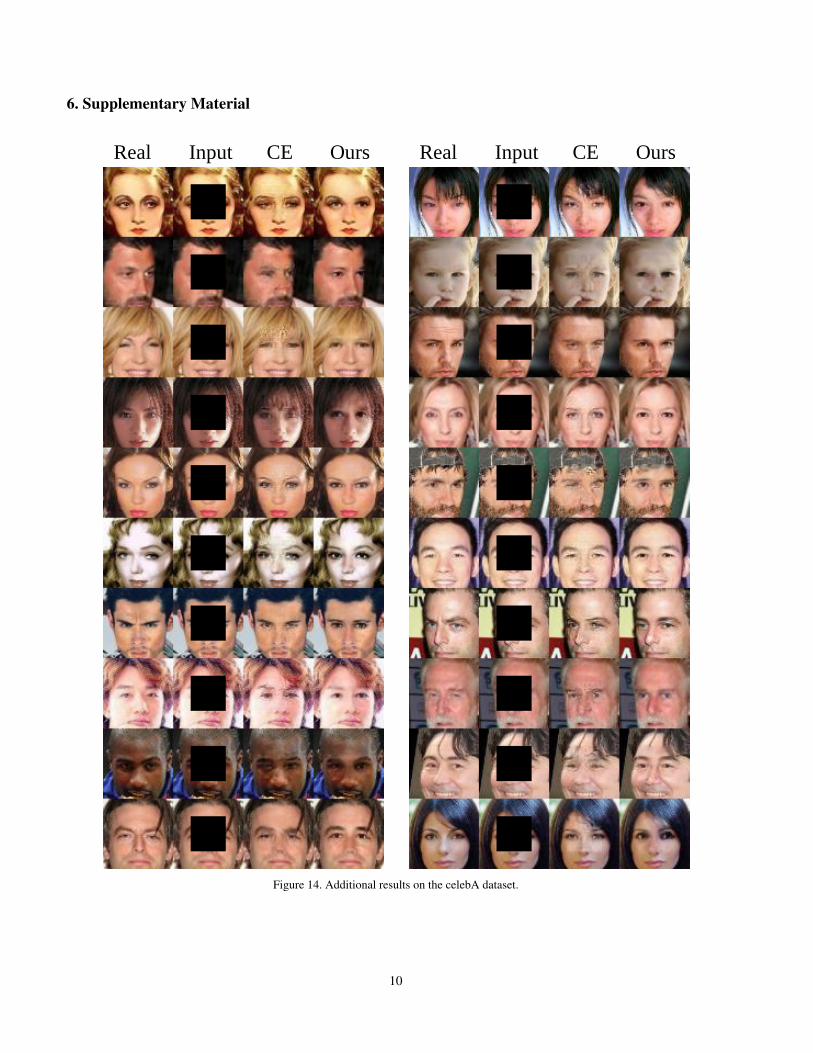
Figure 14. Additional results on the celebA dataset.

10

Real Input CE Ours Real Input CE Ours

Figure 15. Additional results on the celebA dataset.

11

Real Input CE Ours Real Input CE Ours

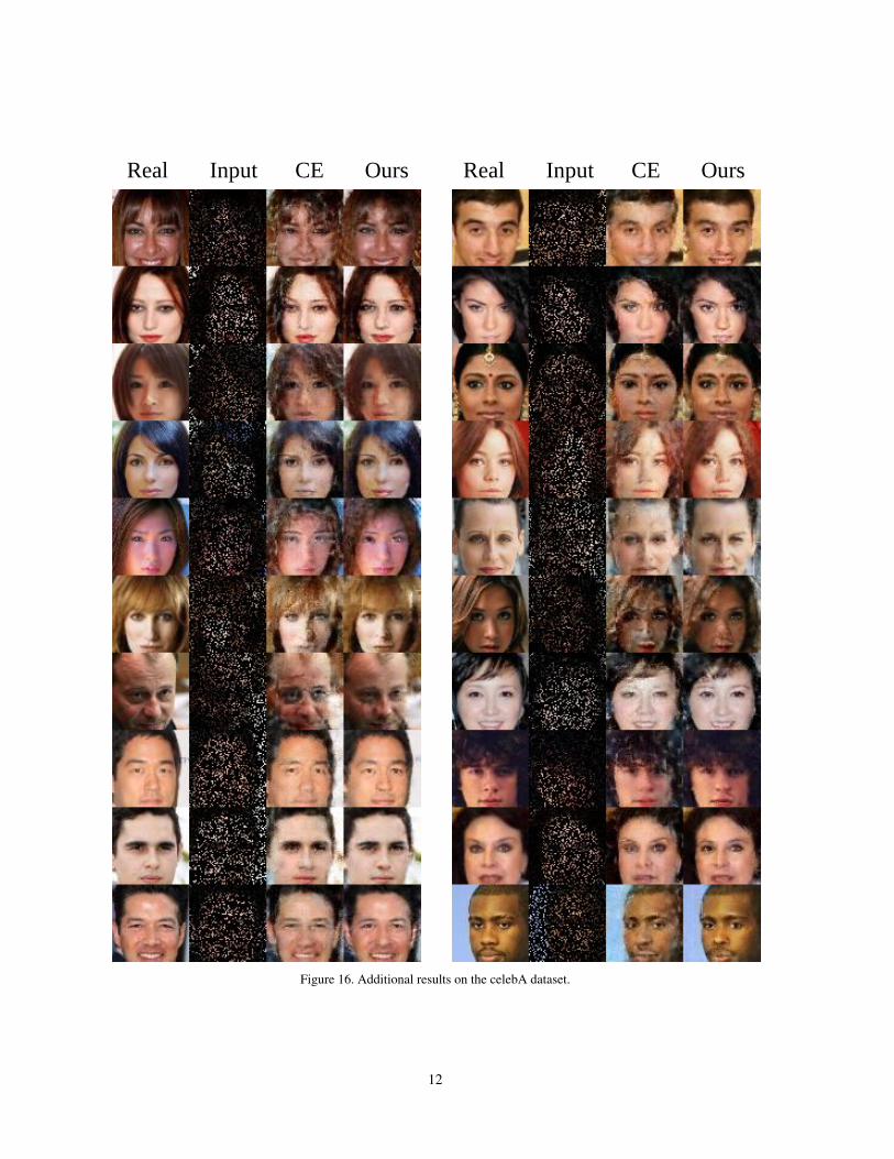
Figure 16. Additional results on the celebA dataset.

12

Real Input CE Ours Real Input CE Ours

Figure 17. Additional results on the celebA dataset.

13

Real Input CE Ours Real Input CE Ours

Figure 18. Additional results on the SVHN dataset.

14

Real Input CE Ours Real Input CE Ours

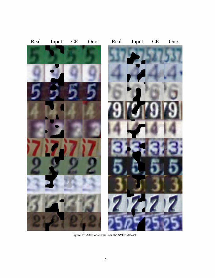
Figure 19. Additional results on the SVHN dataset.

15

Real Input CE Ours Real Input CE Ours

Figure 20. Additional results on the SVHN dataset.

16

Real Input CE Ours Real Input CE Ours

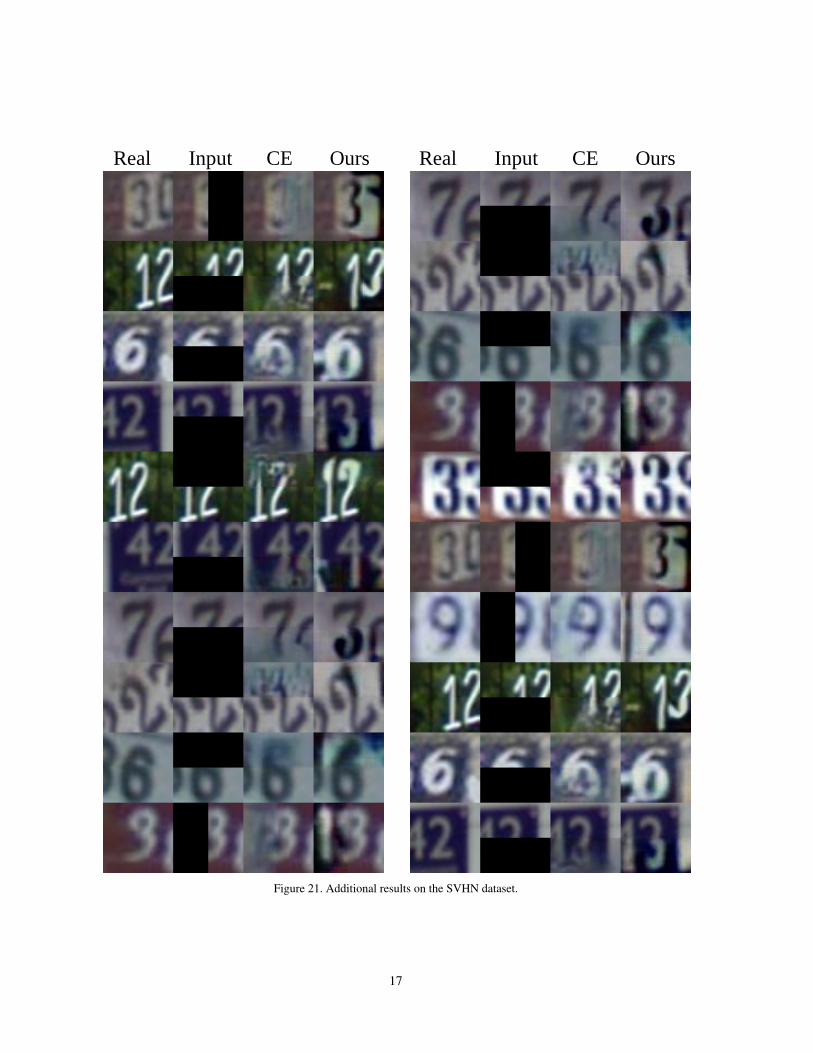
Figure 21. Additional results on the SVHN dataset.

17

Real Input CE Ours Real Input CE Ours

Figure 22. Additional results on the car dataset.

18

Real Input CE Ours Real Input CE Ours

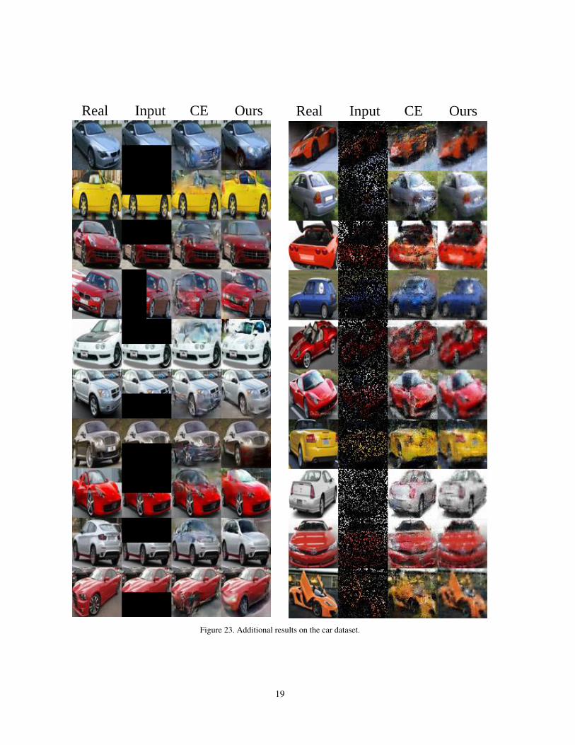
Figure 23. Additional results on the car dataset.

19