Semantic Compositional Networks for Visual...
10
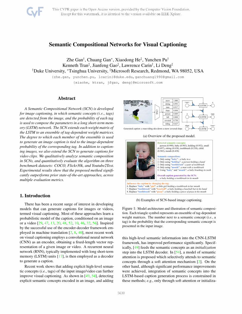
Semantic Compositional Networks for Visual Captioning Zhe Gan † , Chuang Gan * , Xiaodong He ‡ , Yunchen Pu † Kenneth Tran ‡ , Jianfeng Gao ‡ , Lawrence Carin † , Li Deng ‡ † Duke University, * Tsinghua University, ‡ Microsoft Research, Redmond, WA 98052, USA {zhe.gan, yunchen.pu, lcarin}@duke.edu, [email protected] {xiaohe, ktran, jfgao, deng}@microsoft.com Abstract A Semantic Compositional Network (SCN) is developed for image captioning, in which semantic concepts (i.e., tags) are detected from the image, and the probability of each tag is used to compose the parameters in a long short-term mem- ory (LSTM) network. The SCN extends each weight matrix of the LSTM to an ensemble of tag-dependent weight matrices. The degree to which each member of the ensemble is used to generate an image caption is tied to the image-dependent probability of the corresponding tag. In addition to caption- ing images, we also extend the SCN to generate captions for video clips. We qualitatively analyze semantic composition in SCNs, and quantitatively evaluate the algorithm on three benchmark datasets: COCO, Flickr30k, and Youtube2Text. Experimental results show that the proposed method signifi- cantly outperforms prior state-of-the-art approaches, across multiple evaluation metrics. 1. Introduction There has been a recent surge of interest in developing models that can generate captions for images or videos, termed visual captioning. Most of these approaches learn a probabilistic model of the caption, conditioned on an image or a video [29, 47, 13, 20, 48, 52, 10, 46, 32, 56]. Inspired by the successful use of the encoder-decoder framework em- ployed in machine translation [2, 8, 40], most recent work on visual captioning employs a convolutional neural network (CNN) as an encoder, obtaining a fixed-length vector rep- resentation of a given image or video. A recurrent neural network (RNN), typically implemented with long short-term memory (LSTM) units [17], is then employed as a decoder to generate a caption. Recent work shows that adding explicit high-level seman- tic concepts (i.e., tags) of the input image/video can further improve visual captioning. As shown in [49, 54], detecting explicit semantic concepts encoded in an image, and adding LSTM LSTM LSTM CNN snow 1.000 skiing 0.993 man 0.917 slope 0.898 person 0.889 hill 0.808 covered 0.750 riding 0.627 Generated caption: a man riding skis down a snow covered slope a man <eos> a <sos> slope (a) Overview of the proposed model. Detected semantic concepts: person (0.998), baby (0.983), holding (0.952), small (0.697), sitting (0.638), toothbrush (0.538), child (0.502), mouth (0.438) Semantic composition: 1. Only using “baby”: a baby in a 2. Only using “holding”: a person holding a hand 3. Only using “toothbrush”: a pair of toothbrush 4. Only using “mouth”: a man with a toothbrush 5. Using “baby” and “mouth”: a baby brushing its teeth Overall caption generated by the SCN: a baby holding a toothbrush in its mouth Influence the caption by changing the tag: 6. Replace “baby” with “girl”: a little girl holding a toothbrush in her mouth 7. Replace “toothbrush” with “baseball”: a baby holding a baseball bat in his hand 8. Replace “toothbrush” with “pizza”: a baby holding a piece of pizza in his mouth (b) Examples of SCN-based image captioning. Figure 1: Model architecture and illustration of semantic composi- tion. Each triangle symbol represents an ensemble of tag-dependent weight matrices. The number next to a semantic concept (i.e.,a tag) is the probability that the corresponding semantic concept is presented in the input image. this high-level semantic information into the CNN-LSTM framework, has improved performance significantly. Specif- ically, [49] feeds the semantic concepts as an initialization step into the LSTM decoder. In [54], a model of semantic attention is proposed which selectively attends to semantic concepts through a soft attention mechanism [2]. On the other hand, although significant performance improvements were achieved, integration of semantic concepts into the LSTM-based caption generation process is constrained in these methods; e.g., only through soft attention or initializa- 5630
Transcript of Semantic Compositional Networks for Visual...
Semantic Compositional Networks for Visual Captioning
Zhe Gan†, Chuang Gan∗, Xiaodong He‡, Yunchen Pu†
Kenneth Tran‡, Jianfeng Gao‡, Lawrence Carin†, Li Deng‡
†Duke University, ∗Tsinghua University, ‡Microsoft Research, Redmond, WA 98052, USA
{zhe.gan, yunchen.pu, lcarin}@duke.edu, [email protected]
{xiaohe, ktran, jfgao, deng}@microsoft.com
Abstract
A Semantic Compositional Network (SCN) is developed
for image captioning, in which semantic concepts (i.e., tags)
are detected from the image, and the probability of each tag
is used to compose the parameters in a long short-term mem-
ory (LSTM) network. The SCN extends each weight matrix of
the LSTM to an ensemble of tag-dependent weight matrices.
The degree to which each member of the ensemble is used
to generate an image caption is tied to the image-dependent
probability of the corresponding tag. In addition to caption-
ing images, we also extend the SCN to generate captions for
video clips. We qualitatively analyze semantic composition
in SCNs, and quantitatively evaluate the algorithm on three
benchmark datasets: COCO, Flickr30k, and Youtube2Text.
Experimental results show that the proposed method signifi-
cantly outperforms prior state-of-the-art approaches, across
multiple evaluation metrics.
1. Introduction
There has been a recent surge of interest in developing
models that can generate captions for images or videos,
termed visual captioning. Most of these approaches learn a
probabilistic model of the caption, conditioned on an image
or a video [29, 47, 13, 20, 48, 52, 10, 46, 32, 56]. Inspired
by the successful use of the encoder-decoder framework em-
ployed in machine translation [2, 8, 40], most recent work
on visual captioning employs a convolutional neural network
(CNN) as an encoder, obtaining a fixed-length vector rep-
resentation of a given image or video. A recurrent neural
network (RNN), typically implemented with long short-term
memory (LSTM) units [17], is then employed as a decoder
to generate a caption.
Recent work shows that adding explicit high-level seman-
tic concepts (i.e., tags) of the input image/video can further
improve visual captioning. As shown in [49, 54], detecting
explicit semantic concepts encoded in an image, and adding
LSTM
LSTM
LSTM
CN
N
snow 1.000
skiing 0.993
man 0.917
slope 0.898
person 0.889
hill 0.808
covered 0.750
riding 0.627
Generated caption: a man riding skis down a snow covered slope
a
man
<eos>
a
<sos>
slope
(a) Overview of the proposed model.
!
Detected semantic concepts:
person (0.998), baby (0.983), holding (0.952), small
(0.697), sitting (0.638), toothbrush (0.538), child
(0.502), mouth (0.438)
Semantic composition:
1. Only using “baby”: a baby in a
2. Only using “holding”: a person holding a hand
3. Only using “toothbrush”: a pair of toothbrush
4. Only using “mouth”: a man with a toothbrush
5. Using “baby” and “mouth”: a baby brushing its teeth
Overall caption generated by the SCN:
a baby holding a toothbrush in its mouth
Influence the caption by changing the tag:
6. Replace “baby” with “girl”: a little girl holding a toothbrush in her mouth
7. Replace “toothbrush” with “baseball”: a baby holding a baseball bat in his hand
8. Replace “toothbrush” with “pizza”: a baby holding a piece of pizza in his mouth
!
(b) Examples of SCN-based image captioning.
Figure 1: Model architecture and illustration of semantic composi-
tion. Each triangle symbol represents an ensemble of tag-dependent
weight matrices. The number next to a semantic concept (i.e., a
tag) is the probability that the corresponding semantic concept is
presented in the input image.
this high-level semantic information into the CNN-LSTM
framework, has improved performance significantly. Specif-
ically, [49] feeds the semantic concepts as an initialization
step into the LSTM decoder. In [54], a model of semantic
attention is proposed which selectively attends to semantic
concepts through a soft attention mechanism [2]. On the
other hand, although significant performance improvements
were achieved, integration of semantic concepts into the
LSTM-based caption generation process is constrained in
these methods; e.g., only through soft attention or initializa-
15630
tion of the first step of the LSTM.
In this paper, we propose the Semantic Compositional
Network (SCN) to more effectively assemble the meanings
of individual tags to generate the caption that describes the
overall meaning of the image, as illustrated in Figure 1a. Sim-
ilar to the conventional CNN-LSTM-based image captioning
framework, a CNN is used to extract the visual feature vector,
which is then fed into a LSTM for generating the image cap-
tion (for simplicity, in this discussion we refer to images, but
the method is also applicable to video). However, unlike the
conventional LSTM, the SCN extends each weight matrix
of the conventional LSTM to an ensemble of tag-dependent
weight matrices, subject to the probabilities that the tags are
present in the image. These tag-dependent weight matrices
form a weight tensor with a large number of parameters. In
order to make learning feasible, we factorize that tensor to be
a three-way matrix product, which dramatically reduces the
number of free parameters to be learned, while also yielding
excellent performance.
The main contributions of this paper are as follows: (i) We
propose the SCN to effectively compose individual semantic
concepts for image captioning. (ii) We perform compre-
hensive evaluations on two image captioning benchmarks,
demonstrating that the proposed method outperforms previ-
ous state-of-the-art approaches by a substantial margin. For
example, as reported by the COCO official test server, we
achieve a BLEU-4 of 33.1, an improvement of 1.5 points
over the current published state-of-the-art [54]. (iii) We
extend the proposed framework from image captioning to
video captioning, demonstrating the versatility of the pro-
posed model. (iv) We also perform a detailed analysis to
study the SCN, showing that the model can adjust the caption
smoothly by modifying the tags.
2. Related work
We focus on recent neural-network-based literature for
caption generation, as these are most relevant to our work.
Such models typically extract a visual feature vector via a
CNN, and then send that vector to a language model for
caption generation. Representative works include [7, 9, 10,
20, 23, 24, 29, 48] for image captioning and [10, 46, 47,
56, 3, 35, 11] for video captioning. The differences of the
various methods mainly lie in the types of CNN architectures
and language models. For example, the vanilla RNN [12]
was used in [29, 20], while the LSTM [17] was used in [48,
46, 47]. The visual feature vector was only fed into the RNN
once at the first time step in [48, 20], while it was used at
each time step of the RNN in [29].
Most recently, [52] utilized an attention-based mecha-
nism to learn where to focus in the image during caption
generation. This work was followed by [53] which intro-
duced a review module to improve the attention mechanism
and [28] which proposed a method to improve the correct-
ness of visual attention. Moreover, a variational autoencoder
was developed in [34] for image captioning. Other related
work includes [32] for video captioning and [1] for compos-
ing sentences that describe novel objects.
Another class of models uses semantic information for
caption generation. Specifically, [18] applied retrieved
sentences as additional semantic information to guide the
LSTM when generating captions, while [13, 49, 54] applied
a semantic-concept-detection process [15] before generating
sentences. In addition, [13] also proposes a deep multimodal
similarity model to project visual features and captions into
a joint embedding space. This line of methods represents
the current state of the art for image captioning. Our pro-
posed model also lies in this category; however, distinct
from the aforementioned approaches, our model uses weight
tensors in LSTM units. This allows learning an ensemble of
semantic-concept-dependent weight matrices for generating
the caption.
Related to but distinct from the hierarchical composition
in a recursive neural network [37], our model carries out im-
plicit composition of concepts, and there is no hierarchical
relationship among these concepts. Figure 1b illustrates the
semantic composition manifested in the SCN model. Specif-
ically, a set of semantic concepts, such as “baby, holding,
toothbrush, mouth”, are detected with high probabilities. If
only one semantic concept is turned on, the model will gen-
erate a description covering only part of the input image, as
shown in sentences 1-5 of Figure 1b; however, by assem-
bling all these semantic concepts, the SCN is able to generate
a comprehensive description “a baby holding a toothbrush
in its mouth”. More interestingly, as shown in sentences
6-8 of Figure 1b, the SCN also has great flexibility to adjust
the generation of the caption by changing certain semantic
concepts.
The tensor factorization method is used to make the SCN
compact and simplify learning. Similar ideas have been
exploited in [25, 30, 38, 39, 41, 50, 14]. In [10, 19, 23]
the authors also briefly discussed using the tensor factor-
ization method for image captioning. Specifically, visual
features extracted from CNNs are utilized in [10, 23], and
an inferred scene vector is used in [19] for tensor factor-
ization. In contrast to these works, we use the semantic-
concept vector that is formed by the probabilities of all tags
to weight the basis LSTM weight matrices in the ensem-
ble. Our semantic-concept vector is more powerful than
the visual-feature vector [10, 23] and the scene vector [19]
in terms of providing explicit semantic information of an
image, hence leading to significantly better performance,
as shown in our quantitative evaluation. In addition, the
usage of semantic concepts also makes the proposed SCN
more interpretable than [10, 19, 23], as shown in our qualita-
tive analysis, since each unit in the semantic-concept vector
corresponds to an explicit tag.
5631
3. Semantic compositional networks
3.1. Review of RNN for image captioning
Consider an image I, with associated caption X. We
first extract feature vector v(I), which is often the top-layer
features of a pretrained CNN. Henceforth, for simplicity, we
omit the explicit dependence on I, and represent the visual
feature vector as v. The length-T caption is represented as
X = (x1, . . . ,xT ), with xt a 1-of-V (“one hot”) encoding
vector, with V the size of the vocabulary. The length T
typically varies among different captions.
The t-th word in a caption, xt, is linearly embedded into
an nx-dimensional real-valued vector wt = Wext, where
We ∈ Rnx×V is a word embedding matrix (learned), i.e., wt
is a column of We chosen by the one-hot xt. The probability
of caption X given image feature vector v is defined as
p(X|I) =∏T
t=1p(xt|x0, . . . ,xt−1,v) , (1)
where x0 is defined as a special start-of-the-sentence to-
ken. All the words in the caption are sequentially generated
using a RNN, until the end-of-the-sentence symbol is gener-
ated. Specifically, each conditional p(xt|x<t,v) is specified
as softmax(Vht), where ht is recursively updated through
ht = H(wt−1,ht−1,v), and h0 is defined as a zero vector
(h0 is not updated during training). V is the weight matrix
connecting the RNN’s hidden state, used for computing a
distribution over words. Bias terms are omitted for simplicity
throughout the paper.
Without loss of generality, we begin by discussing an
RNN with a simple transition function H(·); this is general-
ized in Section 3.4 to the LSTM. Specifically, H(·) is defined
as
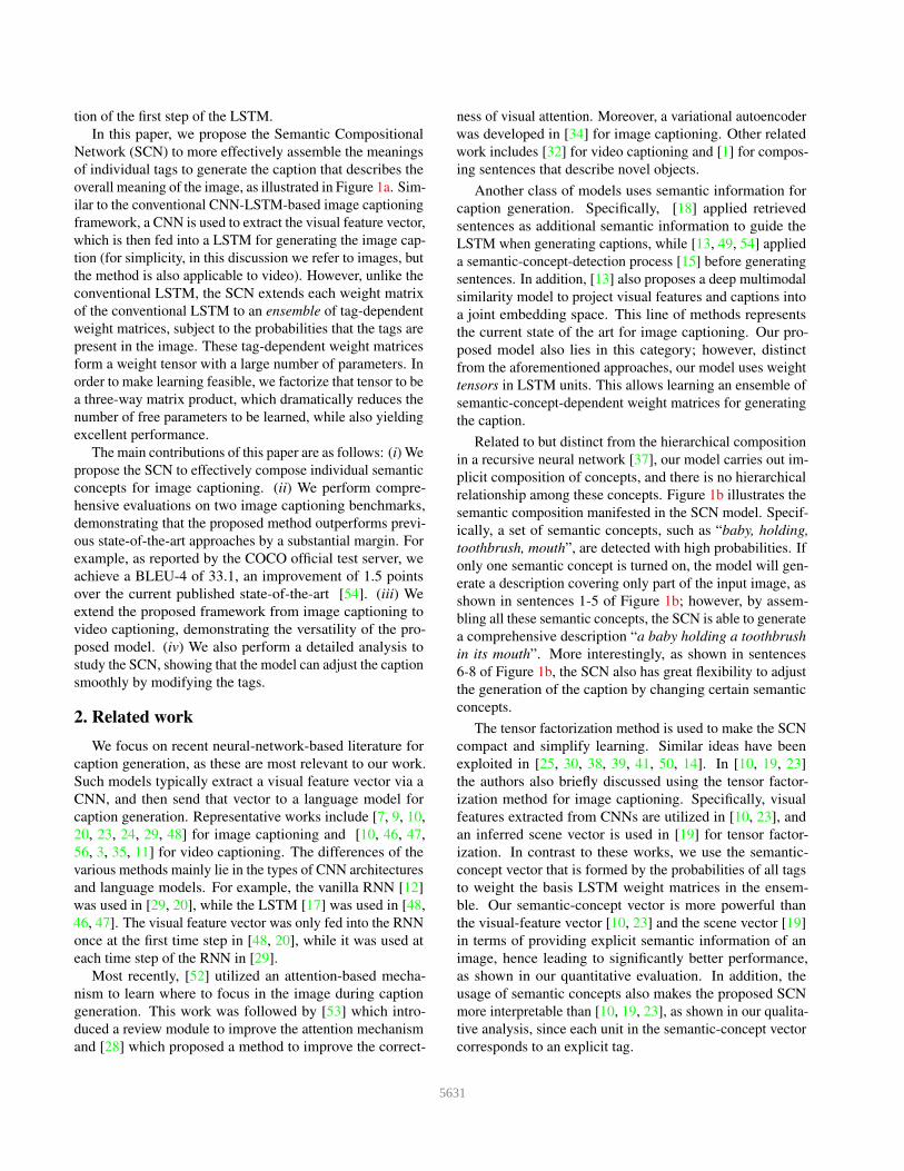
ht = σ(Wxt−1 +Uht−1 + 1(t = 1) ·Cv) , (2)
where σ(·) is a logistic sigmoid function, and 1(·) represents
an indicator function. Feature vector v is fed into the RNN
at the beginning, i.e., at t = 1. W is defined as the input
matrix, and U is termed the recurrent matrix. The model in
(2) is illustrated in Figure 2(a).
3.2. Semantic concept detection
The SCN developed below is based on the detection of
semantic concepts, i.e., tags, in the image under test. In order
to detect such from an image, we first select a set of tags
from the caption text in the training set. Following [13], we
use the K most common words in the training captions to
determine the vocabulary of tags, which includes the most
frequent nouns, verbs, or adjectives.
In order to predict semantic concepts given a test image,
motivated by [49, 44], we treat this problem as a multi-label
classification task. Suppose there are N training examples,
and yi = [yi1, . . . , yiK ] ∈ {0, 1}K is the label vector of the
!
"#
"$%&'"( "&
"& ")
ℎ& ℎ) ℎ$
!
"#
"$%&"( "&
"& ")
ℎ& ℎ) ℎ$
(a) Basic RNN
(b) SCN-RNN
Figure 2: Comparison of our proposed model with a conven-
tional recurrent neural network (RNN) for caption generation. v
and s denote the visual feature and semantic feature, respectively.
x0 represents a special start-of-the-sentence token, (x1, . . . ,xT )represents the caption, and (h1, . . . ,hT ) denotes the RNN hid-
den states. Each triangle symbol represents an ensemble of tag-
dependent weight matrices.
i-th image, where yik = 1 if the image is annotated with tag
k, and yik = 0 otherwise. Let vi and si represent the image
feature vector and the semantic feature vector for the i-th
image, the cost function to be minimized is
1
N
N∑
i=1
K∑
k=1
(
yik log sik + (1− yik) log(1− sik))
, (3)
where si = σ(
f(vi))
is a K-dimensional vector with si =[si1, . . . , siK ], σ(·) is the logistic sigmoid function and f(·)is implemented as a multilayer perceptron (MLP).
In testing, for each input image, we compute a semantic-
concept vector s, formed by the probabilities of all tags,
computed by the semantic-concept detection model.
3.3. SCN-RNN
The SCN extends each weight matrix of the conventional
RNN to be an ensemble of a set of tag-dependent weight
matrices, subjective to the probabilities that the tags are
present in the image. Specifically, the SCN-RNN computes
the hidden states as follows
ht = σ(W(s)xt−1 +U(s)ht−1 + z) , (4)
where z = 1(t = 1) · Cv, and W(s) and U(s) are en-
sembles of tag-dependent weight matrices, subjective to the
probabilities that the tags are present in the image, according
to the semantic-concept vector s.
Given s ∈ RK , we define two weight tensors WT ∈
Rnh×nx×K and UT ∈ R
nh×nh×K , where nh is the number
5632
of hidden units and nx is the dimension of word embedding.
W(s) ∈ Rnh×nx and U(s) ∈ R
nh×nh can be specified as
W(s) =
K∑
k=1
skWT [k], U(s) =
K∑
k=1
skUT [k] , (5)
where sk is the k-th element in s; WT [k] and UT [k] denote
the k-th 2D “slice” of WT and UT , respectively. The prob-
ability of the k-th semantic concept, sk, is associated with a
pair of RNN weight matrices WT [k] and UT [k], implicitly
specifying K RNNs in total. Consequently, training such a
model as defined in (4) and (5) can be interpreted as jointly
training an ensemble of K RNNs.
Though appealing, the number of parameters is propor-
tional to K, which is prohibitive for large K (e.g., K = 1000for COCO). In order to remedy this problem, we adopt ideas
from [30] to factorize W(s) and U(s) defined in (5) as
W(s) = Wa · diag(Wbs) ·Wc , (6)
U(s) = Ua · diag(Ubs) ·Uc , (7)
where Wa ∈ Rnh×nf , Wb ∈ R
nf×K and Wc ∈ Rnf×nx .
Similiarly, Ua ∈ Rnh×nf , Ub ∈ R
nf×K and Uc ∈ Rnf×nh .
nf is the number of factors. Substituting (6) and (7) into (4),
we obtain our SCN with an RNN as
x̃t−1 = Wbs⊙Wcxt−1 , (8)
h̃t−1 = Ubs⊙Ucht−1 , (9)
z = 1(t = 1) ·Cv , (10)
ht = σ(Wax̃t−1 +Uah̃t−1 + z) . (11)
where ⊙ denotes the element-wise multiply (Hadamard)
operator.
Wa and Wc are shared among all the captions, effec-
tively capturing common linguistic patterns; while the di-
agonal term, diag(Wbs), accounts for semantic aspects of
the image under test, captured by s. The same analysis also
holds true for Ua,b,c. In this factorized model, the RNN
weight matrices that correspond to each semantic concept
share “structure.” This factorized model (termed SCN-RNN)
is illustrated in Figure 2(b).
To provide further motivation for and insight into the
decompositions in (6) and (7), let wbk represent the kth
column of Wb, then
W(s) =∑K
k=1sk[Wa · diag(wbk) ·Wc] . (12)
A similar decomposition is manifested for U(s). The matrix
Wa ·diag(wbk)·Wc may be interpreted as the k-th “slice” of
a weight tensor, with each slice corresponding to one of the
K semantic concepts (K total tensor “slices,” each of size
nh × nx). Hence, via the decomposition in (6) and (7), we
effectively learn an ensemble of K sets of RNN parameters,
one for each semantic concept. This is efficiently done by
sharing Wa and Wc when composing each member of the
ensemble. The weight with which the k-th slice of this
tensor contributes to the RNN parameters for a given image
is dependent on the respective probability sk with which the
k-th semantic concept is inferred to be associated with image
I.
The number of parameters in the basic RNN model (see
Figure 2(a)) is nh·(nx+nh), while the number of parameters
in the SCN-RNN model (see Figure 2(b)) is nf · (nx +2K + 3nh). In experiments, we set nf = nh. Therefore,
the additional number of parameters is 2 · nh · (nh + K).This increased model complexity also indicates increased
training/testing time.
3.4. SCN-LSTM
RNNs with LSTM units [17] have emerged as a popular
architecture, due to their representational power and effec-
tiveness at capturing long-term dependencies. We generalize
the SCN-RNN model by using LSTM units. Specifically, we
define ht = H(xt−1,ht−1,v, s) as
it = σ(Wiax̃i,t−1 +Uiah̃i,t−1 + z) , (13)
f t = σ(Wfax̃f,t−1 +Ufah̃f,t−1 + z) , (14)
ot = σ(Woax̃o,t−1 +Uoah̃o,t−1 + z) , (15)
c̃t = σ(Wcax̃c,t−1 +Ucah̃c,t−1 + z) , (16)
ct = it ⊙ c̃t + f t ⊙ ct−1 , (17)
ht = ot ⊙ tanh(ct) , (18)
where z = 1(t = 1) ·Cv. For ⋆ = i, f, o, c, we define
x̃⋆,t−1 = W⋆bs⊙W⋆cxt−1 , (19)
h̃⋆,t−1 = U⋆bs⊙U⋆cht−1 . (20)
Since we implement the SCN with LSTM units, we name
this model SCN-LSTM. In experiments, since LSTM is more
powerful than classifical RNN, we only report results using
SCN-LSTM.
In summary, distinct from previous image-captioning
methods, our model has a unique way to utilize and combine
the visual feature v and semantic-concept vector s extracted
from an image I. v is fed into the LSTM to initialize the first
step, which is expected to provide the LSTM an overview
of the image content. While the LSTM state is initialized
with the overall visual context v, an ensemble of K sets of
LSTM parameters is utilized when decoding, weighted by
the semantic-concept vector s, to generate the caption.
Model learning Given the image I and associated caption
X, the objective function is the sum of the log-likelihood of
the caption conditioned on the image representation:
log p(X|I) =∑T
t=1p(xt|x0, . . . ,xt−1,v, s) . (21)
5633
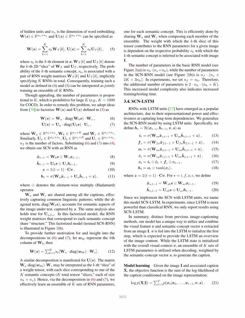
MethodsCOCO Flickr30k
B-1 B-2 B-3 B-4 M C B-1 B-2 B-3 B-4 M
NIC [48] 0.666 0.451 0.304 0.203 − − 0.663 0.423 0.277 0.183 −m-RNN [29] 0.67 0.49 0.35 0.25 − − 0.60 0.41 0.28 0.19 −Hard-Attention [52] 0.718 0.504 0.357 0.250 0.230 − 0.669 0.439 0.296 0.199 0.185
ATT [54] 0.709 0.537 0.402 0.304 0.243 − 0.647 0.460 0.324 0.230 0.189
Att-CNN+LSTM [49] 0.74 0.56 0.42 0.31 0.26 0.94 0.73 0.55 0.40 0.28 −LSTM-R 0.698 0.525 0.390 0.292 0.238 0.889 0.657 0.437 0.296 0.201 0.186
LSTM-T 0.716 0.546 0.411 0.312 0.250 0.952 0.691 0.483 0.336 0.232 0.202
LSTM-RT 0.724 0.555 0.419 0.316 0.252 0.970 0.706 0.486 0.339 0.235 0.204
LSTM-RT2 0.730 0.568 0.430 0.322 0.249 0.977 0.724 0.523 0.370 0.257 0.210
SCN-LSTM 0.728 0.566 0.433 0.330 0.257 1.012 0.735 0.530 0.377 0.265 0.218
SCN-LSTM Ensemble of 5 0.741 0.578 0.444 0.341 0.261 1.041 0.747 0.552 0.403 0.288 0.223
Table 1: Performance of the proposed model (SCN-LSTM) and other state-of-the-art methods on the COCO and Flickr30k datasets, where
B-N , M and C are short for BLEU-N , METEOR and CIDEr-D scores, respectively.
The above objective corresponds to a single image-caption
pair. In training, we average over all training pairs.
3.5. Extension to video captioning
The above framework can be readily extended to the
task of video captioning [10, 46, 47, 56, 3, 51]. In order
to effectively represent the spatiotemporal visual content
of a video, we use a two-dimensional (2D) and a three-
dimensional (3D) CNN to extract visual features of video
frames/clips. We then perform a mean pooling process [47]
over all 2D CNN features and 3D CNN features, to generate
two feature vectors (one from 2D CNN features and the
other from 3D CNN features). The representation of each
video, v, is produced by concatenating these two features.
Similarly, we also obtain the semantic-concept vector s by
running the semantic-concept detector based on the video
representation v. After v and s are obtained, we employ
the same model proposed above directly for video-caption
generation, as described in Figure 2(b).
4. Experiments
4.1. Datasets
We present results on three benchmark datasets:
COCO [27], Flickr30k [55] and Youtube2Text [5]. COCO
and Flickr30k are for image captioning, containing 123287
and 31783 images, respectively. Each image is annotated
with at least 5 captions. We use the same pre-defined splits
as [20] for all the datasets: on Flickr30k, 1000 images for
validation, 1000 for test, and the rest for training; and for
COCO, 5000 images are used for both validation and testing.
We further tested our model on the official COCO test set
consisting of 40775 images (human-generated captions for
this split are not publicly available), and evaluated our model
on the COCO evaluation server. We also follow the publicly
available code [20] to preprocess the captions, yielding vo-
cabulary sizes of 8791 and 7414 for COCO and Flickr30k,
respectively.
Youtube2Text is used for video captioning, which con-
tains 1970 Youtube clips, and each video is annotated with
around 40 sentences. We use the same splits as provided
in [47], with 1200 videos for training, 100 videos for valida-
tion, and 670 videos for testing. We convert all captions to
lower case and remove the punctuation, yielding vocabulary
size of 12594 for Youtube2Text.
4.2. Training procedure
For image representation, we take the output of the 2048-
way pool5 layer from ResNet-152 [16], pretrained on the
ImageNet dataset [36]. For video representation, in addition
to using the 2D ResNet-152 to extract features on each video
frame, we also utilize a 3D CNN (C3D) [43] to extract
features on each video. The C3D is pretrained on Sports-1M
video dataset [21], and we take the output of the 4096-way
fc7 layer from C3D as the video representation. We consider
the RGB frames of videos as input, with 2 frames per second.
Each video frame is resized as 112× 112 and 224× 224 for
the C3D and ResNet-152 feature extractor, respectively. The
C3D feature extractor is applied on video clips of length 16
frames (as in [21]) with an overlap of 8 frames.
We use the procedure described in Section 3.2 for se-
mantic concept detection. The semantic-concept vocabulary
size is determined to reflect the complexity of the dataset,
which is set to 1000, 200 and 300 for COCO, Flickr30k and
Youtube2Text, respectively. Since Youtube2Text is a rela-
tively small dataset, we found that it is very difficult to train
a reliable semantic-concept detector using the Youtube2Text
dataset alone, due to its limited amount of data. In experi-
ments, we utilize additional training data from COCO.
For model training, all the parameters in the SCN-LSTM
are initialized from a uniform distribution in [-0.01,0.01].
All bias terms are initialized to zero. Word embedding vec-
tors are initialized with the publicly available word2vec vec-
tors [31]. The embedding vectors of words not present in the
5634
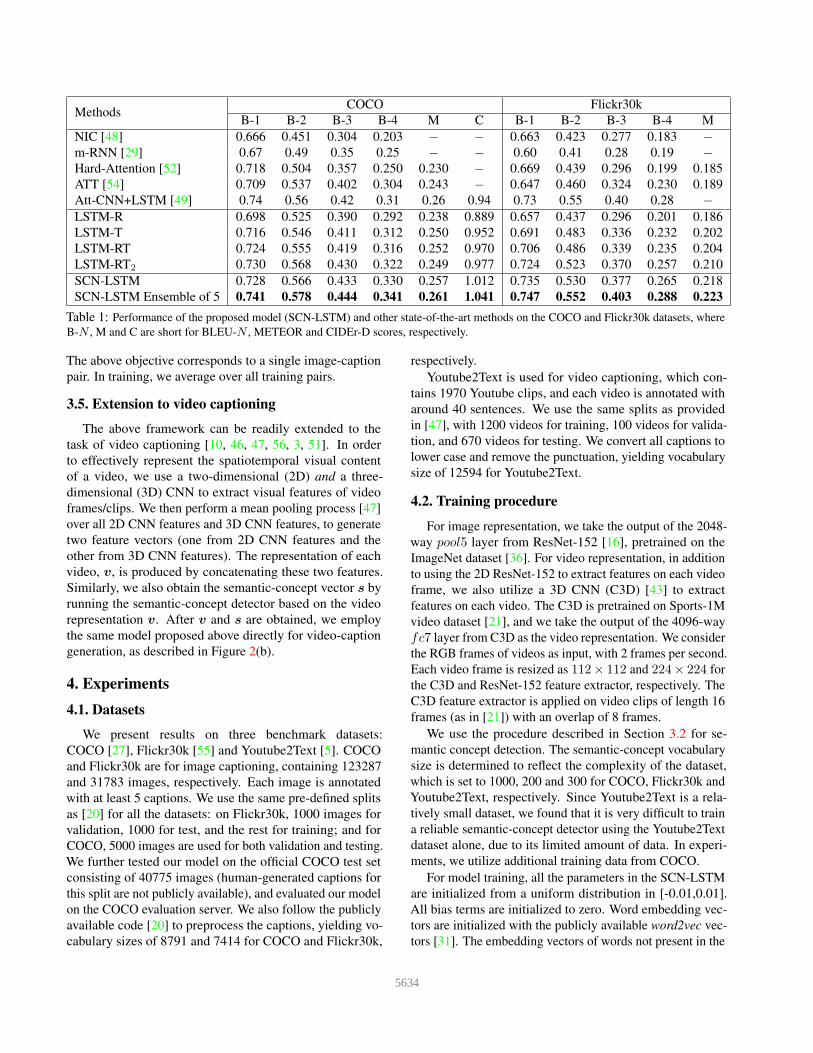
ModelBLEU-1 BLEU-2 BLEU-3 BLEU-4 METEOR ROUGE-L CIDEr-D
c5 c40 c5 c40 c5 c40 c5 c40 c5 c40 c5 c40 c5 c40
SCN-LSTM 0.740 0.917 0.575 0.839 0.436 0.739 0.331 0.631 0.257 0.348 0.543 0.696 1.003 1.013
ATT 0.731 0.900 0.565 0.815 0.424 0.709 0.316 0.599 0.250 0.335 0.535 0.682 0.943 0.958
OV 0.713 0.895 0.542 0.802 0.407 0.694 0.309 0.587 0.254 0.346 0.530 0.682 0.943 0.946
MSR Cap 0.715 0.907 0.543 0.819 0.407 0.710 0.308 0.601 0.248 0.339 0.526 0.680 0.931 0.937
Table 2: Comparison to published state-of-the-art image captioning models on the blind test set as reported by the COCO test server.
SCN-LSTM is our model. ATT refers to ATT VC [54], OV refers to OriolVinyals [48], and MSR Cap refers to MSR Captivator [9].
Model B-4 M C
S2VT [46] − 0.292 −
LSTM-E [32] 0.453 0.310 −
GRU-RCN [3] 0.479 0.311 0.678
h-RNN [56] 0.499 0.326 0.658
LSTM-R 0.448 0.310 0.640
LSTM-C 0.445 0.309 0.644
LSTM-CR 0.469 0.317 0.688
LSTM-T 0.473 0.324 0.699
LSTM-CRT 0.475 0.316 0.647
LSTM-CRT2 0.469 0.326 0.706
SCN-LSTM 0.502 0.334 0.770
SCN-LSTM Ensemble of 5 0.511 0.335 0.777
Table 3: Results on BLEU-4 (B-4), METEOR (M) and CIDEr-D
(C) metrices compared to other state-of-the-art results and baselines
on Youtube2Text.
pretrained set are initialzied randomly. The number of hid-
den units and the number of factors in SCN-LSTM are both
set to 512 and we use mini-batches of size 64. The maxi-
mum number of epochs we run for all the three datasets is 20.
Gradients are clipped if the norm of the parameter vector ex-
ceeds 5 [40]. We do not perform any dataset-specific tuning
and regularization other than dropout [57] and early stopping
on validation sets. The Adam algorithm [22] with learning
rate 2× 10⁻⁴ is utilized for optimization. All experiments
are implemented in Theano [42]1.
In testing, we use beam search for caption generation,
which selects the top-k best sentences at each time step and
considers them as the candidates to generate new top-k best
sentences at the next time step. We set the beam size to
k = 5 in experiments.
4.3. Evaluation
The widely used BLEU [33], METEOR [4], ROUGE-
L [26], and CIDEr-D [45] metrics are reported in our quanti-
tative evaluation of the performance of the proposed model
and baselines in the literature. All the metrics are com-
puted by using the code released by the COCO evalua-
tion server [6]. For COCO and Flickr30k datasets, besides
comparing to results reported in previous work, we also re-
implemented strong baselines for comparison. The results
of image captioning are presented in Table 1. The models
we implemented are as follows.
1Code is publicly available at https://github.com/zhegan27/
Semantic_Compositional_Nets.
1. LSTM-R / LSTM-T / LSTM-RT: R, T, RT denotes us-
ing different features. Specifically, R denotes ResNet
visual feature vector, T denotes Tags (i.e., the semantic-
concept vector), and RT denotes the concatenation of R
and T. The features are fed into a standard LSTM de-
coder only at the initial time step. In particular, LSTM-T
is the model proposed in [49].
2. LSTM-RT2: The ResNet feature vector is sent to a stan-
dard LSTM decoder at the first time step, while the tag
vector is sent to the LSTM decoder at every time step in
addition to the input word. This model is similar to [54]
without using semantic attention. This is the model
closest to ours, which provides a direct comparison to
our proposed model.
3. SCN-LSTM: This is the model presented in Section 3.4.
For video captioning experiments, we use the same no-
tation. For example, LSTM-C means we leverage the C3D
feature for caption generation.
4.4. Quantitative results
Performance on COCO and Flickr30k We first present
results on the task of image captioning, summarized in Ta-
ble 1. The use of tags (LSTM-T) provides better performance
than leveraging visual features alone (LSTM-R). Combining
both tags and visual features further enhances performance,
as expected. Compared with only feeding the tags into the
LSTM at the initial time step (LSTM-RT), LSTM-RT2 yields
better results, since it takes as input the tag feature at each
time step. Further, the direct comparison between LSTM-RT2
and SCN-LSTM demonstrates the advantage of our proposed
model, indicating that our approach is a better method to
fuse semantic concepts into the LSTM.
We also report results averaging an ensemble of 5 identi-
cal SCN-LSTM models trained with different initializations,
which is a common strategy adopted widely [54] (note that
now we employ ensembles in two ways: an ensemble of
LSTM parameters linked to tags, and an overaching ensem-
ble atop the entire model). We obtain state-of-the-art results
on both COCO and Flickr30k datasets. Remarkably, we
improve the state-of-the-art BLEU-4 score by 3.1 points on
COCO.
Performance on COCO test server We also evaluate the
proposed SCN-LSTM model by uploading results to the on-
5635
!
Tags:
dog (1), grass (0.996),
laying (0.97), outdoor
(0.943), next (0.788),
sitting (0.651), lying
(0.542), white (0.507) !
Tags:
road (1), decker (1), double
(0.999), bus (0.996), red
(0.996), street (0.926),
building (0.859), driving
(0.796) !
Tags:
zebra (1), animal (0.985),
mammal (0.948), dirt
(0.937), grass (0.902),
standing (0.878), group
(0.848), field (0.709)
Caption generated by our model:
a dog laying on the ground next to a frisbee
Semantic composition:
1. Replace “dog” with “cat”:
a white cat laying on the ground
2. Replace “grass” with “bed”:
a white dog laying on top of a bed
3. Replace “grass” with “laptop”:
a dog laying on the ground next to a laptop!
Caption generated by our model:
a red double decker bus driving down a street
Semantic composition:
1. Replace “red” with “blue”:
a blue double decker bus driving down a street
2. Replace “bus” with “train”:
a red train traveling down a city street
3. Replace “road” and “street” with “ocean”:
a red bus is driving in the ocean!
Caption generated by our model:
a herd of zebra standing on top of a dirt field
Semantic composition:
1. Replace “zebra” with “horse”:
a group of horses standing in a field
2. Replace “standing” with “running”:
a herd of zebra running across a dirt field
3. Replace “field” with “snow”:
a group of zebras standing in the snow!
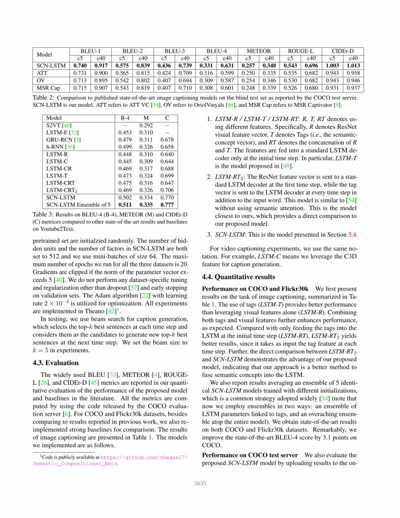
!Figure 3: Illustration of semantic composition. Our model can adjust the caption smoothly as the semantic concepts are modified.
!
Tags:
indoor (0.952), dog
(0.828), sitting (0.647),
stuffed (0.602), white
(0.544), next (0.527),
laying (0.509), cat (0.402)! !
Tags:
snow(1), outdoor (0.992),
covered (0.847), nature
(0.812), skiing (0.61), man
(0.451), pile (0.421),
building (0.369) !
Tags:
person (1), cabinet (0.931),
man (0.906), shelf (0.771),
table (0.707), front (0.683),
holding (0.662), food
(0.587)
Generated captions:
SCN-LSTM-T: a dog laying on top of a stuffed
animal
SCN-LSTM: a teddy bear laying on top of a
stuffed animal!
Generated captions:
SCN-LSTM-T: a person that is standing in the
snow
SCN-LSTM: a stop sign is covered in the snow!
Generated captions:
SCN-LSTM-T: a man sitting at a table with a
plate of food
SCN-LSTM: a man is holding a glass of wine!
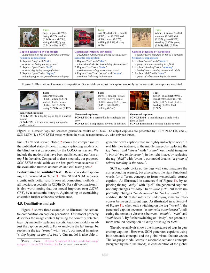
!Figure 4: Detected tags and sentence generation results on COCO. The output captions are generated by: 1) SCN-LSTM, and 2)
SCN-LSTM-T, a SCN-LSTM model without the visual feature inputs, i.e., with only tag inputs.
line COCO test server. Table 2 shows the comparison to
the published state-of-the-art image captioning models on
the blind test set as reported by the COCO test server. We
include the models that have been published and perform at
top-3 in the table. Compared to these methods, our proposed
SCN-LSTM model achieves the best performance across all
the evaluation metrics on both c5 and c40 testing sets.2
Performance on Youtube2Text Results on video caption-
ing are presented in Table 3. The SCN-LSTM achieves
significantly better results over all competing methods in
all metrics, especially in CIDEr-D. For self-comparison, it
is also worth noting that our model improves over LSTM-
CRT2 by a substantial margin. Again, using an overaching
ensemble further enhances performance.
4.5. Qualitative analysis
Figure 3 shows three examples to illustrate the seman-
tic composition on caption generation. Our model properly
describes the image content by using the correctly detected
tags. By manually replacing specific tags, our model can ad-
just the caption smoothly. For example, in the left image, by
replacing the tag “grass” with “bed”, our model imagines
“a dog laying on top of a bed”. Our model is also able to
2Please check https://competitions.codalab.org/
competitions/3221#results for the most recent results.
generate novel captions that are highly unlikely to occur in
real life. For instance, in the middle image, by replacing the
tag “road” and “street” with “ocean”, our model imagines
“a bus driving in the ocean”; in the right image, by replacing
the tag “field” with “snow”, our model dreams “a group of
zebras standing in the snow”.
SCN not only picks up the tags well (and imagines the
corresponding scenes), but also selects the right functional
words for different concepts to form syntactically correct
caption. As illustrated in sentence 6 of Figure 1b, by re-
placing the tag “baby” with “girl”, the generated captions
not only changes “a baby” to “a little girl”, but more im-
portantly, changes “in its mouth” to “in her mouth”. In
addition, the SCN also infers the underlying semantic relat-
edness between different tags. As illustrated in sentence 4
of Figure 1b, when only switching on the tag “mouth”, the
generated caption becomes “a man with a toothbrush”, indi-
cating the semantic closeness between “mouth”, “man” and
“toothbrush”. By further switching on “baby”, we generate a
more detailed description “a baby brushing its teeth”.
The above analysis shows the importance of tags in gen-
erating captions. However, SCN generates captions using
both semantic concepts and the global visual feature vector.
The language model learns to assemble semantic concepts
(weighted by their likelihood), in consideration of the global
5636
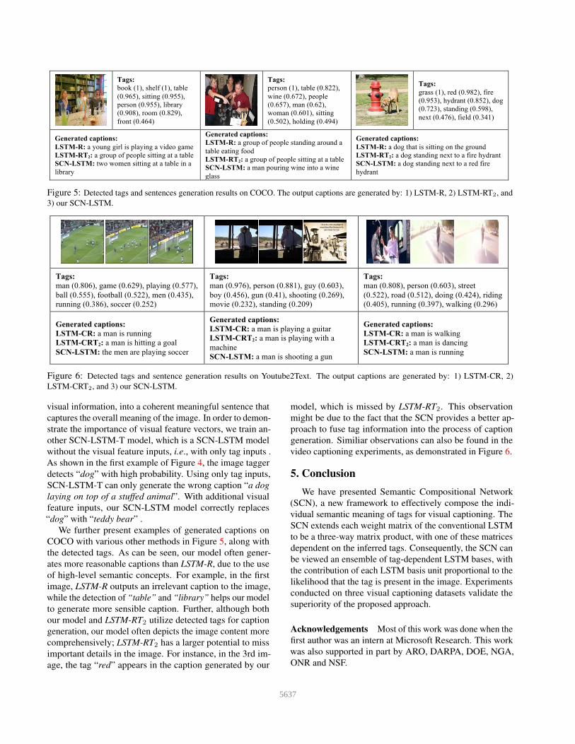
!
Tags:
book (1), shelf (1), table
(0.965), sitting (0.955),
person (0.955), library
(0.908), room (0.829),
front (0.464) !
Tags:
person (1), table (0.822),
wine (0.672), people
(0.657), man (0.62),
woman (0.601), sitting
(0.502), holding (0.494) !
Tags:
grass (1), red (0.982), fire
(0.953), hydrant (0.852), dog
(0.723), standing (0.598),
next (0.476), field (0.341)
Generated captions:
LSTM-R: a young girl is playing a video game
LSTM-RT2: a group of people sitting at a table
SCN-LSTM: two women sitting at a table in a
library!
Generated captions:
LSTM-R: a group of people standing around a
table eating food
LSTM-RT2: a group of people sitting at a table
SCN-LSTM: a man pouring wine into a wine
glass!
Generated captions:
LSTM-R: a dog that is sitting on the ground
LSTM-RT2: a dog standing next to a fire hydrant
SCN-LSTM: a dog standing next to a red fire
hydrant!
!Figure 5: Detected tags and sentences generation results on COCO. The output captions are generated by: 1) LSTM-R, 2) LSTM-RT2, and
3) our SCN-LSTM.
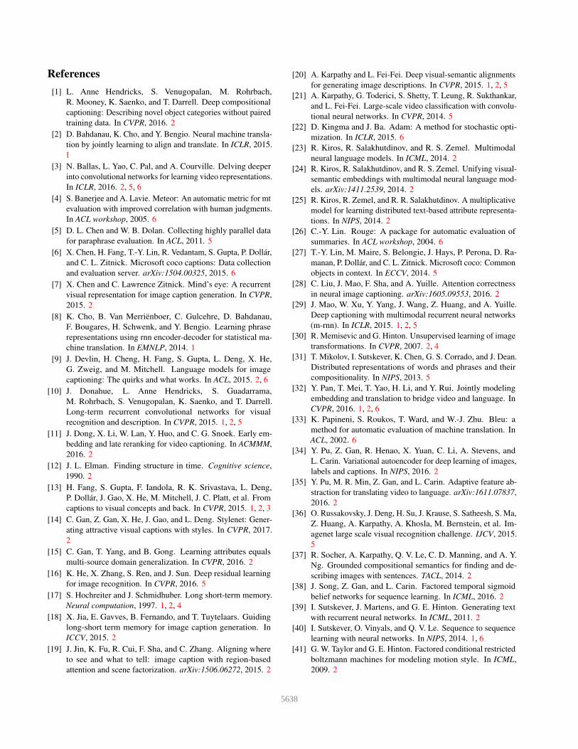
!
Tags:
man (0.806), game (0.629), playing (0.577),
ball (0.555), football (0.522), men (0.435),
running (0.386), soccer (0.252)!
Tags:
man (0.976), person (0.881), guy (0.603),
boy (0.456), gun (0.41), shooting (0.269),
movie (0.232), standing (0.209)
Tags:
man (0.808), person (0.603), street
(0.522), road (0.512), doing (0.424), riding
(0.405), running (0.397), walking (0.296)
Generated captions:
LSTM-CR: a man is running
LSTM-CRT2: a man is hitting a goal
SCN-LSTM: the men are playing soccer!
Generated captions:
LSTM-CR: a man is playing a guitar
LSTM-CRT2: a man is playing with a
machine
SCN-LSTM: a man is shooting a gun
Generated captions:
LSTM-CR: a man is walking
LSTM-CRT2: a man is dancing
SCN-LSTM: a man is running
!Figure 6: Detected tags and sentence generation results on Youtube2Text. The output captions are generated by: 1) LSTM-CR, 2)
LSTM-CRT2, and 3) our SCN-LSTM.
visual information, into a coherent meaningful sentence that
captures the overall meaning of the image. In order to demon-
strate the importance of visual feature vectors, we train an-
other SCN-LSTM-T model, which is a SCN-LSTM model
without the visual feature inputs, i.e., with only tag inputs .
As shown in the first example of Figure 4, the image tagger
detects “dog” with high probability. Using only tag inputs,
SCN-LSTM-T can only generate the wrong caption “a dog
laying on top of a stuffed animal”. With additional visual
feature inputs, our SCN-LSTM model correctly replaces
“dog” with “teddy bear” .
We further present examples of generated captions on
COCO with various other methods in Figure 5, along with
the detected tags. As can be seen, our model often gener-
ates more reasonable captions than LSTM-R, due to the use
of high-level semantic concepts. For example, in the first
image, LSTM-R outputs an irrelevant caption to the image,
while the detection of “table” and “library” helps our model
to generate more sensible caption. Further, although both
our model and LSTM-RT2 utilize detected tags for caption
generation, our model often depicts the image content more
comprehensively; LSTM-RT2 has a larger potential to miss
important details in the image. For instance, in the 3rd im-
age, the tag “red” appears in the caption generated by our
model, which is missed by LSTM-RT2. This observation
might be due to the fact that the SCN provides a better ap-
proach to fuse tag information into the process of caption
generation. Similiar observations can also be found in the
video captioning experiments, as demonstrated in Figure 6.
5. Conclusion
We have presented Semantic Compositional Network
(SCN), a new framework to effectively compose the indi-
vidual semantic meaning of tags for visual captioning. The
SCN extends each weight matrix of the conventional LSTM
to be a three-way matrix product, with one of these matrices
dependent on the inferred tags. Consequently, the SCN can
be viewed an ensemble of tag-dependent LSTM bases, with
the contribution of each LSTM basis unit proportional to the
likelihood that the tag is present in the image. Experiments
conducted on three visual captioning datasets validate the
superiority of the proposed approach.
Acknowledgements Most of this work was done when the
first author was an intern at Microsoft Research. This work
was also supported in part by ARO, DARPA, DOE, NGA,
ONR and NSF.
5637
References
[1] L. Anne Hendricks, S. Venugopalan, M. Rohrbach,
R. Mooney, K. Saenko, and T. Darrell. Deep compositional
captioning: Describing novel object categories without paired
training data. In CVPR, 2016. 2
[2] D. Bahdanau, K. Cho, and Y. Bengio. Neural machine transla-
tion by jointly learning to align and translate. In ICLR, 2015.
1
[3] N. Ballas, L. Yao, C. Pal, and A. Courville. Delving deeper
into convolutional networks for learning video representations.
In ICLR, 2016. 2, 5, 6
[4] S. Banerjee and A. Lavie. Meteor: An automatic metric for mt
evaluation with improved correlation with human judgments.
In ACL workshop, 2005. 6
[5] D. L. Chen and W. B. Dolan. Collecting highly parallel data
for paraphrase evaluation. In ACL, 2011. 5
[6] X. Chen, H. Fang, T.-Y. Lin, R. Vedantam, S. Gupta, P. Dollár,
and C. L. Zitnick. Microsoft coco captions: Data collection
and evaluation server. arXiv:1504.00325, 2015. 6
[7] X. Chen and C. Lawrence Zitnick. Mind’s eye: A recurrent
visual representation for image caption generation. In CVPR,
2015. 2
[8] K. Cho, B. Van Merriënboer, C. Gulcehre, D. Bahdanau,
F. Bougares, H. Schwenk, and Y. Bengio. Learning phrase
representations using rnn encoder-decoder for statistical ma-
chine translation. In EMNLP, 2014. 1
[9] J. Devlin, H. Cheng, H. Fang, S. Gupta, L. Deng, X. He,
G. Zweig, and M. Mitchell. Language models for image
captioning: The quirks and what works. In ACL, 2015. 2, 6
[10] J. Donahue, L. Anne Hendricks, S. Guadarrama,
M. Rohrbach, S. Venugopalan, K. Saenko, and T. Darrell.
Long-term recurrent convolutional networks for visual
recognition and description. In CVPR, 2015. 1, 2, 5
[11] J. Dong, X. Li, W. Lan, Y. Huo, and C. G. Snoek. Early em-
bedding and late reranking for video captioning. In ACMMM,
2016. 2
[12] J. L. Elman. Finding structure in time. Cognitive science,
1990. 2
[13] H. Fang, S. Gupta, F. Iandola, R. K. Srivastava, L. Deng,
P. Dollár, J. Gao, X. He, M. Mitchell, J. C. Platt, et al. From
captions to visual concepts and back. In CVPR, 2015. 1, 2, 3
[14] C. Gan, Z. Gan, X. He, J. Gao, and L. Deng. Stylenet: Gener-
ating attractive visual captions with styles. In CVPR, 2017.
2
[15] C. Gan, T. Yang, and B. Gong. Learning attributes equals
multi-source domain generalization. In CVPR, 2016. 2
[16] K. He, X. Zhang, S. Ren, and J. Sun. Deep residual learning
for image recognition. In CVPR, 2016. 5
[17] S. Hochreiter and J. Schmidhuber. Long short-term memory.
Neural computation, 1997. 1, 2, 4
[18] X. Jia, E. Gavves, B. Fernando, and T. Tuytelaars. Guiding
long-short term memory for image caption generation. In
ICCV, 2015. 2
[19] J. Jin, K. Fu, R. Cui, F. Sha, and C. Zhang. Aligning where
to see and what to tell: image caption with region-based
attention and scene factorization. arXiv:1506.06272, 2015. 2
[20] A. Karpathy and L. Fei-Fei. Deep visual-semantic alignments
for generating image descriptions. In CVPR, 2015. 1, 2, 5
[21] A. Karpathy, G. Toderici, S. Shetty, T. Leung, R. Sukthankar,
and L. Fei-Fei. Large-scale video classification with convolu-
tional neural networks. In CVPR, 2014. 5
[22] D. Kingma and J. Ba. Adam: A method for stochastic opti-
mization. In ICLR, 2015. 6
[23] R. Kiros, R. Salakhutdinov, and R. S. Zemel. Multimodal
neural language models. In ICML, 2014. 2
[24] R. Kiros, R. Salakhutdinov, and R. S. Zemel. Unifying visual-
semantic embeddings with multimodal neural language mod-
els. arXiv:1411.2539, 2014. 2
[25] R. Kiros, R. Zemel, and R. R. Salakhutdinov. A multiplicative
model for learning distributed text-based attribute representa-
tions. In NIPS, 2014. 2
[26] C.-Y. Lin. Rouge: A package for automatic evaluation of
summaries. In ACL workshop, 2004. 6
[27] T.-Y. Lin, M. Maire, S. Belongie, J. Hays, P. Perona, D. Ra-
manan, P. Dollár, and C. L. Zitnick. Microsoft coco: Common
objects in context. In ECCV, 2014. 5
[28] C. Liu, J. Mao, F. Sha, and A. Yuille. Attention correctness
in neural image captioning. arXiv:1605.09553, 2016. 2
[29] J. Mao, W. Xu, Y. Yang, J. Wang, Z. Huang, and A. Yuille.
Deep captioning with multimodal recurrent neural networks
(m-rnn). In ICLR, 2015. 1, 2, 5
[30] R. Memisevic and G. Hinton. Unsupervised learning of image
transformations. In CVPR, 2007. 2, 4
[31] T. Mikolov, I. Sutskever, K. Chen, G. S. Corrado, and J. Dean.
Distributed representations of words and phrases and their
compositionality. In NIPS, 2013. 5
[32] Y. Pan, T. Mei, T. Yao, H. Li, and Y. Rui. Jointly modeling
embedding and translation to bridge video and language. In
CVPR, 2016. 1, 2, 6
[33] K. Papineni, S. Roukos, T. Ward, and W.-J. Zhu. Bleu: a
method for automatic evaluation of machine translation. In
ACL, 2002. 6
[34] Y. Pu, Z. Gan, R. Henao, X. Yuan, C. Li, A. Stevens, and
L. Carin. Variational autoencoder for deep learning of images,
labels and captions. In NIPS, 2016. 2
[35] Y. Pu, M. R. Min, Z. Gan, and L. Carin. Adaptive feature ab-
straction for translating video to language. arXiv:1611.07837,
2016. 2
[36] O. Russakovsky, J. Deng, H. Su, J. Krause, S. Satheesh, S. Ma,
Z. Huang, A. Karpathy, A. Khosla, M. Bernstein, et al. Im-
agenet large scale visual recognition challenge. IJCV, 2015.
5
[37] R. Socher, A. Karpathy, Q. V. Le, C. D. Manning, and A. Y.
Ng. Grounded compositional semantics for finding and de-
scribing images with sentences. TACL, 2014. 2
[38] J. Song, Z. Gan, and L. Carin. Factored temporal sigmoid
belief networks for sequence learning. In ICML, 2016. 2
[39] I. Sutskever, J. Martens, and G. E. Hinton. Generating text
with recurrent neural networks. In ICML, 2011. 2
[40] I. Sutskever, O. Vinyals, and Q. V. Le. Sequence to sequence
learning with neural networks. In NIPS, 2014. 1, 6
[41] G. W. Taylor and G. E. Hinton. Factored conditional restricted
boltzmann machines for modeling motion style. In ICML,
2009. 2
5638
[42] Theano Development Team. Theano: A Python framework
for fast computation of mathematical expressions. arXiv:
1605.02688, 2016. 6
[43] D. Tran, L. Bourdev, R. Fergus, L. Torresani, and M. Paluri.
Learning spatiotemporal features with 3d convolutional net-
works. In ICCV, 2015. 5
[44] K. Tran, X. He, L. Zhang, J. Sun, C. Carapcea, C. Thrasher,
C. Buehler, and C. Sienkiewicz. Rich image captioning in the
wild. In CVPR Workshops, 2016. 3
[45] R. Vedantam, C. Lawrence Zitnick, and D. Parikh. Cider:
Consensus-based image description evaluation. In CVPR,
2015. 6
[46] S. Venugopalan, M. Rohrbach, J. Donahue, R. Mooney,
T. Darrell, and K. Saenko. Sequence to sequence-video to
text. In ICCV, 2015. 1, 2, 5, 6
[47] S. Venugopalan, H. Xu, J. Donahue, M. Rohrbach, R. Mooney,
and K. Saenko. Translating videos to natural language using
deep recurrent neural networks. In NAACL, 2015. 1, 2, 5
[48] O. Vinyals, A. Toshev, S. Bengio, and D. Erhan. Show and
tell: A neural image caption generator. In CVPR, 2015. 1, 2,
5, 6
[49] Q. Wu, C. Shen, L. Liu, A. Dick, and A. v. d. Hengel. What
value do explicit high level concepts have in vision to lan-
guage problems? In CVPR, 2016. 1, 2, 3, 5, 6
[50] Y. Wu, S. Zhang, Y. Zhang, Y. Bengio, and R. Salakhutdinov.
On multiplicative integration with recurrent neural networks.
In NIPS, 2016. 2
[51] J. Xu, T. Mei, T. Yao, and Y. Rui. Msr-vtt: A large video
description dataset for bridging video and language. In CVPR,
2016. 5
[52] K. Xu, J. Ba, R. Kiros, K. Cho, A. Courville, R. Salakhut-
dinov, R. S. Zemel, and Y. Bengio. Show, attend and tell:
Neural image caption generation with visual attention. In
ICML, 2015. 1, 2, 5
[53] Z. Yang, Y. Yuan, Y. Wu, R. Salakhutdinov, and W. W. Cohen.
Review networks for caption generation. In NIPS, 2016. 2
[54] Q. You, H. Jin, Z. Wang, C. Fang, and J. Luo. Image cap-
tioning with semantic attention. In CVPR, 2016. 1, 2, 5,
6
[55] P. Young, A. Lai, M. Hodosh, and J. Hockenmaier. From im-
age descriptions to visual denotations: New similarity metrics
for semantic inference over event descriptions. TACL, 2014.
5
[56] H. Yu, J. Wang, Z. Huang, Y. Yang, and W. Xu. Video para-
graph captioning using hierarchical recurrent neural networks.
In CVPR, 2016. 1, 2, 5, 6
[57] W. Zaremba, I. Sutskever, and O. Vinyals. Recurrent neural
network regularization. arXiv:1409.2329, 2014. 6
5639