Electronic copy available at: http://ssrn.com/abstract=2799749

Selling a Product Line Through a Retailer When Demand is

Stochastic: Analysis of Price-Only Contracts

Lingxiu Dong, Xiaomeng Guo, and Danko Turcic

Olin Business School, Washington University in St. Louis, St. Louis, MO 63130

June 23, 2016

Abstract

To expand sales, many manufacturers try to develop and sell product lines. Frequently, however, the

operations of distributing a product line creates tension between manufacturers and retailers as they

do not necessarily agree on which product versions included in the product line should be sold to

consumers. To mitigate this tension, previous literature has shown that if a manufacturer (he) wants to

sell his product line through a retailer (she) who faces deterministic demand, then he needs to adjust

his product qualities according to her requirements; otherwise she will not carry the entire line. In

contrast, this paper shows that if demand is stochastic, then a manufacturer can mitigate the same

tension merely by re-allocating inventory risk in the supply chain. This strategy can be so effective that

it is possible to find cases where the equilibrium product line is actually longer in a decentralized supply

chain than in the direct-selling case. To understand the tradeoff, we consider a supply chain with a

manufacturer capable of producing multiple product designs and a retailer who faces stochastic consumer

demand. The manufacturer sells his output through the retailer using one of the following variations

on the classical wholesale contract: push (PH), pull (PL), or instantaneous fulfillment (IF). With PH

and PL (IF), wholesale prices and quantities are decided before (after) demand is revealed. Retail

prices are always set after demand is revealed. With PH (PL) the retailer (manufacturer) carries retail

inventory. Taking the manufacturer’s point of view, we characterize the equilibrium product line length

and equilibrium contracting strategy. Our answers are determined by three important drivers: demand

variability, product substitutability, and the retailer’s outside option. Low outside option and low (high)

substitutability imply that the manufacturer maximizes his expected profit offering the retailer longer

(shorter) product line using the IF contract. As outside option increases, the equilibrium contract will

be either PH or PL. High demand variability and low substitutability imply that the manufacturer

should be expected to sell a longer product line with a PH contract. Low demand variability and high

substitutability imply that the manufacturer should be expected to sell a shorter product line with a

PL contract.

Electronic copy available at: http://ssrn.com/abstract=2799749

1 Introduction

To facilitate sales growth and to induce cross-selling, many manufacturers design and produce prod-

ucts in product lines rather than in single product variants. 1 Implementing a successful product line

strategy, however, can become challenging for a manufacturer who sells his output through an inde-

pendent retailer because such a manufacturer does not control the assortment and stocking decisions

at the retail location. While he may attempt to influence these decisions, e.g., through pricing, they

both are ultimately made by the retailer who cares about her own profits. Such a retailer may choose

to carry not more than a subset of the manufacturer’s product line and stock smaller quantities of

each product version than what the manufacturer would prefer. This occurrence is widespread. To

illustrate, consider Oberweis Dairy, which serves the Greater St. Louis, MO-IL metropolitan area.

Oberweis has a long product line, which includes four types of milk, five flavors of ice-cream cakes,

over forty flavors of ice cream, and several flavors of yogurt. Although the full product line is avail-

able at retail locations, which Oberweis operates, independent grocery chains tend to carry only one

or two Oberweis’ ice cream flavors and a limited selection of Oberweis’ milk. Further examples from

popular business press mention manufacturers who want to extend their product lines in order to

increase sales and retailers who are only interested in offering limited selections of “best sellers.” The

grocery chain Kroger Co., for example, stripped about 30% of its cereal varieties made by companies

like Kelloggs and General Mills (Brat et al., 2009). To motivate retailers to carry their products,

manufacturers run sales promotions (Nijs et al., 2010; Yuan et al., 2013) or even tailor product de-

signs to the needs of individual retailers (Villas-Boas, 1998). However, empirical research reveals

that the effectiveness of some of these practices – the practice of sales promotions in particular – is

not completely clear (Kumar et al., 2001; Nijs et al., 2010).

Recent research in marketing and economics has done an excellent job of formally documenting

the aforementioned tension in a setting where retail demand is deterministic and the manufacturer

delivers his output to the retailer with zero lead time (Villas-Boas, 1998; Liu and Cui, 2010). Taken

together, these assumptions are conducive to studying the product line length (or assortment) ques-

tion without having to consider the retailer’s stocking decisions. (Since the retailer stocks what she

1Definition: A product line is a group of products that are closely related to each other by function and price. Inoffering a product line, manufacturers often use common components or building blocks to create derivative offeringsthat target various consumer preferences.

2

sells.) One of the central findings in this literature is that if a manufacturer wants to sell a product

line through a retailer, then he needs to adjust his product qualities according to her requirements;

otherwise the retailer will drop some products included in the product line (see Villas-Boas, 1998;

Liu and Cui, 2010).

In contrast, the inventory and supply chain literature studied the previously mentioned tension

in a setting where the manufacturer produces a single product design, delivery lead times are strictly

positive, retail demand is stochastic, and retail prices are fixed. Taken together, these assumptions are

fitting for studying the stocking question, but are not necessarily conducive to studying the questions

of product variety and the retailer’s incentive to carry a product line. One of the important findings

in this literature is that the choice of a supply contract type (supply contract types differ in pricing,

lead times, and inventory risk allocation) affects the retailer’s stocking decision (see Cachon, 2003,

for a survey of this large literature).

However, when product assortment decisions are combined with inventory decisions in the pres-

ence of uncertain demand, existing theories do not necessarily lend themselves to answering the

overarching question of how to engage a retailer who chooses not only how much to sell but also what

to sell. Would the manufacturer offer the retailer a product line or just a single product? Would the

manufacturer deliver the goods with zero lead time (as it is assumed in the product line literature)

or would the manufacturer quote the retailer a longer lead time, giving rise to inventory?2 If quoting

long lead time is the optimal choice for the manufacturer, how would the inventory risk be optimally

allocated and how would that affect the product line length?

The thesis behind this paper is that answering these questions requires a new model – one that

combines stochastic demand, lead time choice, endogenous pricing, and assortment planning at both

ends of the supply chain. In this paper, we propose a stylized version of one such model. In particular,

our model is a bilateral supply chain where a manufacturer sells up to two differentiated product

designs through a retailer to consumers. Consumer demand is linear and stochastic. At time 0, only

the distribution of future demand is known. At time 1, demand outcome is known, and is controlled

by the retail price set by the retailer.

2Note that zero delivery lead times allow both firms to wait for demand to be revealed before committing to pricesand quantities. However, an argument given in Iyer et al. (2007) suggests that a manufacturer selling a single productdesign may benefit from exposing the retailer to inventory risk. Therefore it is unclear that zero lead time is alwayspreferable to the manufacturer.

3

We consider a supply chain with an upstream manufacturer (he) capable of producing multiple

product designs and a downstream retailer (she) who faces stochastic demand. Each product design

that the manufacturer decides to produce requires a costly setup and can be delivered to the retail

location with zero lead time or depending on the manufacturer’s delivery lead time choice. The

manufacturer makes a “take-it-or-leave-it” wholesale contract offer to the retailer, subject to leaving

her with some minimum acceptable expected payoff. This payoff may be seen as a reservation

utility that the retailer could achieve by pursuing another opportunity, e.g., by carrying a different

manufacturer’s product line. For this reason, we refer to this as the retailer’s outside option. (For

an empirical manifestation of outside options, see Ailawadi, 2001; Bloom and Perry, 2001.)

We consider three variations of the wholesale contract: push, pull, or instantaneous fulfillment.

Throughout the paper, prices, quantities, and product line length are all endogenous and product

qualities are exogenous. This is because our main interest is in the oper of distributing a product

line rather than in designing one.

The wholesale contract variations differ in the timing of quantity and pricing decisions: Retail

prices are always set after demand is revealed. Wholesale prices, product line length, and stocking

quantities are decided before demand is revealed if the contract is push or pull; with instantaneous

fulfillment, they are all set after demand is revealed. Push and pull, however, differ in how they

allocate inventory risk. With push (pull), inventory risk is with the retailer (manufacturer). Finally,

in terms of lead times, with push and pull, the production lead time is 1 and with instantaneous

fulfillment, the production lead time is 0.

All three contracts are simple because each has a single wholesale price per product version. It is

plausible that firms may restrict attention to these simple contracts, especially because more complex

alternatives such as buy-backs do not coordinate in our setting even when the product line length

is reduced to a single product. Those contracts run into trouble because the incentive they provide

to coordinate the retailer’s quantity action distorts the retailer’s pricing decision (see Cachon, 2003,

§3).

Using our model, we illustrate how optimal inventory decisions interact with optimal product

line length in the presence of stochastic demand. Surprisingly, our results reveal that the manufac-

turer can incentivize the retailer to carry a longer product line not necessarily by designing products

according to the retailer’s requirements (a recommendation put forth in the literature with determin-

4

istic retail demand) but by re-allocating inventory risk in the supply chain. Moreover, this strategy

can be so effective that it is possible to find cases where the equilibrium product line is actually longer

in a decentralized supply chain than in the direct-selling case.

To begin the investigation, we imagine a world in which the supply chain is vertically integrated,

and refer to this setting as integrated supply chain. We show that in such a world, the manufacturer’s

most preferred mode of operation is to utilize his zero lead time capability, wait for demand realization

and then decide which designs to produce and set the production quantity and the retail price of

each design. Waiting gives the manufacturer better information about demand, which has a direct,

positive effect on his profits due to improved efficiency of matching assortment and quantity with

demand. In particular, waiting eliminates cases in which the manufacturer incurs a setup cost for

products, which appear profitable ex ante, but turn out to be unprofitable ex post. We find a range

of setup costs for which the manufacturer operating under the integrated supply chain wants to

produce and sell a greater variety of products so as to achieve increased sales without having to cut

retail price significantly.

When facing the same setup cost in a decentralized supply chain, the manufacturer can again

choose to wait for demand to be revealed by utilizing the instantaneous fulfillment contract. However,

there is also an indirect, strategic effect of waiting that negatively affects the manufacturer’s profits

as it can lead to too high double-marginalization and too high retail prices. We find that the high

double-marginalization makes the instantaneous fulfillment contract particularly unappealing to a

retailer with an attractive outside option. Therefore the manufacturer would not always want to

utilize the instantaneous fulfillment even if producing and delivering goods with zero lead time could

be done costlessly.

When facing a retailer with an attractive outside option, the manufacturer will either announce

the number of product versions and their wholesale prices before demand is revealed and let the

retailer pull the products she decides to sell from his inventory after demand is revealed (pull con-

tract). Or, the manufacturer will announce the number of product versions and their wholesale prices

before demand is revealed and ask the retailer to respond with strictly positive order quantities for

all products that she decides to carry (push contract). We find that the former is a high-price-low-

quantity strategy whereas the latter is a low-price-high-quantity strategy; the former is dominated

by the latter as demand becomes more variable, in which case the wholesale demand is relatively

5

more elastic (i.e., the retailer becomes more responsive to the manufacturer’s wholesale price cut

under the push contract).

By committing to product line before demand uncertainty is resolved, push and pull contracts

respectively expose the retailer and the manufacturer to the inventory risk. Thus, the bearer of the

inventory risk has an incentive to have a longer product line which can serve as a hedge against

the demand uncertainty. We show that under demand uncertainty the equilibrium product line may

become longer in a decentralized supply chain than in a centralized one. This result complements

previous findings of a shorter product line reported in studies that assumed deterministic demand

(Villas-Boas, 1998; Netessine and Taylor, 2007).

Finally, we find that the length of the product line not only depends on product substitutability

but also on contract choices, when substitutability is in the mid-range. Everything else being equal,

lower substitutability and higher demand variability point to a longer product line offered under

push contract; higher substitutability and lower demand variability point to a shorter product line

offered under pull contract.

We conclude our study by constructing a simple numerical example that illustrates how much

better the manufacturer can do by being able to adjust his product line length and to change the

contract type. The data shows that the manufacturer’s expected payoff can increase by more than

60%, which illustrates that both decisions generate first-order effects.

2 Related Literature

There are three areas of literature related to this paper: The literature on supply chain management

with price-only contracts, the literature on inventory models with demand substitution, and the

literature on product line design in distribution channels.

In supply chains managed with price-only contracts, manufacturers sell their output to retailers

who stock the manufacturer’s output and re-sell it to consumers; manufacturers retain the wholesale

revenue while retailers keep the retail revenue. Lariviere and Porteus (2001); Cachon (2004) study

price-only contracts in the context of the newsvendor problem. Because the retailers in the newsven-

dor setting are unable to adjust either retail prices or the retail assortment, managing profits at the

retail location becomes about setting an order quantity that matches supply and demand: Too much

6

supply (demand) leads to lower profits due to excessive inventory costs (excessive opportunity costs

of lost margins). In contrast, the retailer in our paper manages her expected profits by optimizing

not only over order quantities but also over assortment and retail prices. Endogenous assortment de-

cision and retail pricing introduce new forces into the manufacturer-retailer interaction. First, unlike

a newsvendor whose revenue would increase by having more inventory, a retailer with price-sensitive

demand benefits from a higher inventory when the retail demand is elastic (necessities tend to have

inelastic demand while luxuries are more elastic). Second, a manufacturer selling to a newsvendor

fares best as demand variability approaches zero, because double-marginalization reduces as the de-

mand variability decreases (Lariviere and Porteus, 2001). In contrast, a manufacturer selling to a

price-setting retailer would not necessarily want to have a supply chain where demand uncertainty

can be completely avoided even if adopting such a supply chain would be costless (see our explana-

tion in Section 1; additional explanation can found in Iyer et al., 2007). Third, adjusting assortment

gives the retailer another lever to manage demand uncertainty: Everything else being equal, retail

assortment increases with the variability of demand, because a larger product variety can serve as

a hedge against not knowing, which designs will be in high demand. Finally, building upon Cachon

(2004), which studies how the allocation of inventory risk impacts both supply chain inventory and

supply chain efficiency, we find that the allocation of inventory risk affects not only inventory levels

but also retail assortment. That is, push contract and pull contract can result in different retail

assortment.

Several literatures build on the above newsvendor supply chain models. The literature on in-

ventory financing, for example, combines the analysis of inventory risk with financing consideration

(e.g., see Caldentey and Chen, 2012; Yang and Birge, 2013; Kouvelis and Zhao, 2012; Babich and

Tang, 2012; Chod, 2015). We are related to this literature because the contracts we study can also be

viewed as financing contracts. Namely, with the push contract, the retailer pays the manufacturer

before demand is revealed whereas in the pull contract, the retailer pays the manufacturer after

demand is reveal. Therefore the pull contract could be interpreted as a financing contract. Similarly,

the contracts we study are also broadly related to the literature on demand forecasting. In particular,

by choosing the push contract, the firms can be seen as giving up a demand signal. In contrast, by

choosing the either PL or IF contract, either the retailer or both firms make quantity and pricing de-

cisions after receiving a perfect demand signal. Thus by avoiding the push contract, the manufacturer

7

institutes an information-enabled supply chain. The incentives to invest into information-enabled

supply chain is one of the central questions studied in the literature on demand forecasting (e.g., see

Taylor, 2006; Taylor and Xiao, 2008; Shin and Tunca, 2010; Guo and Iyer, 2010). We differ from

this literature by focusing on the joint assortment and stocking problem.

In addition to the single-item newsvendor model, there is a long literature on assortment planning,

multi-item inventory systems, and product line design (e.g. van Ryzin and Mahajan, 1999; Gaur and

Honhon, 2006; Netessine and Taylor, 2007; Aydin and Porteus, 2008; Liu and Cui, 2010). Netessine

and Taylor (2007), for example, study the effect of production technology on a firm’s product line

design strategies with an Economic Order Quantity model; Aydin and Porteus (2008) analyze a

newsvendor’s optimal price and inventory choice of a given assortment; and Alptekinoglu and Corbett

(2010) analyze a firm’s integrated product line design problem that involves variety, leadtime (or

inventory), and pricing decision. Some of the earlier research (Cachon et al., 2005) is reviewed in

Kok et al. (2009). Unlike in these papers, however, the manufacturer in our model operates in a

decentralized supply chain. Everything else being equal, we find that the manufacturer may choose

a shorter or a longer product line when he sells through a retailer, and product line decision and

contract decision interact.

Finally, the analysis in this paper is also related to the literature on product line design for dis-

tribution channels. Villas-Boas (1998) and Liu and Cui (2010) study this problem in settings where

demand is deterministic and delivery lead times are zero. They find that the length of the manufac-

turer’s optimal product line changes (shortens in most cases) when going from a centralized channel

to a decentralized one. Villas-Boas (1998) also argues that to expand the product line, the manufac-

turer’s best strategy is to re-design it. In this paper, we find that with stochastic demand, product

line expansion can be achieved by re-allocating demand risk in the channel, which the manufacturer

achieves by switching between the instantaneous, push, and pull systems. Interestingly, we report

that the retailer might actually choose to carry a longer product line in the decentralized channel

than what the manufacturer choose to sell in the centralized channel (for a detailed explanation of

this result, see our results in Section 5.2).

To summarize, although there is a rich literature on single product distribution in supply chains

with stochastic demand, the incentive problems that arise in distributing a product line have been

understudied and it is something that we do in this paper. Taking the manufacturer’s point of

8

view, we characterize the equilibrium product line length and equilibrium contracting strategy. Our

answers are determined by three important drivers: demand variability, product substitutability,

and the retailer’s outside option. Lengthening product line, at its core, is about increasing sales

without having to cut price significantly. With uncertain demand, low product substitutability

incentivizes the manufacturer to supply a longer product line which can serve as a hedge against

demand uncertainty; so much so that the manufacturer may produce a longer product line when he

sells through an independent retailer than when he sells directly to consumers. In the contracting

space, low outside option makes it more likely that the equilibrium contract will be instantaneous

fulfillment. As outside option increases, the equilibrium contract will be either push or pull; push is

preferred over pull when the manufacturer faces elastic wholesale demand, which can be driven by

increasing variability in retail demand.

The rest of the paper is organized as follows. The next section describes the model. Sections

4 characterizes the equilibrium in a world in which the manufacturer is able to sell directly to

consumers or is able to achieve a first-best vertically integrated supply chain. Section 5 describes the

solution in a world where the supply chain is decentralized and characterizes the subgame-perfect

Nash equilibrium (SPNE) in a game in which the manufacturer can choose which contract to adopt

and the retailer can choose which products to carry. Section 6 concludes.

3 Model

Consider a supply chain where a manufacturer (he) has the capability to produce up to two different

product designs, which he sells through a retailer (she) to consumers. Consumer demand at retail

prices p = (p1, p2) will be denoted by s(p,A). When viewed from time 0, A = (A1, A2) takes on one

of the four possible values, (1 + u, 1 + u), (1 + u, 1− u), (1− u, 1 + u), or (1− u, 1− u), with equal

probability. Thus A is a proxy for demand uncertainty due to factors such as consumer valuation or

market size, and u measures the demand variation. The value of A is fully resolved when consumer

demand clears, which is at time 1. The direct demand s(p,A) has an inverse p (s,A) such that

p (s,A) = (A1 − αs1 − βs2, A2 − βs1 − αs2) . (1)

9

Equation (1) is a familiar inverse demand model proposed by Singh and Vives (1984); variants of this

model have been used by many authors. The term α ≥ 0 measures how own outputs affect prices

while the term β ≥ 0 measures product substitutability. The goods are substitutes or independent

according to whether β > 0 or β = 0. 3 The substitutability effects in this system are identical across

the inverse demand curves. (For a careful derivation of (1) from a consumer utility model, see Singh

and Vives, 1984, p.547 or Ingene and Parry, 2004, p.23.) To ensure that both products are viable,

the substitutability effect cannot be too large. Therefore we adopt the following Assumption 1.

Assumption 1. 0 ≤ β < α 1−u1+u , where α > 0 and 0 ≤ u ≤ 1.

The manufacturer can choose between offering zero, one, or two product versions. To add a

product version to his product line, the manufacturer has to invest a fixed cost f ≥ 0, independent

of the amount produced. The fixed cost, f , captures costly production setups 4 (e.g., Netessine and

Taylor, 2007; Liu and Cui, 2010; Nasser et al., 2013), or marketing costs associated with adding a

new product 5 (e.g., Copple, 2002). The marginal production cost for the manufacturer is normalized

to zero without further loss of generality. The manufacturer’s output can be delivered to the retail

location with zero lead time at no additional cost, depending on the manufacturer’s lead time choice.

We analyze two supply chains: An integrated supply chain and a decentralized one, where the

former serves as a benchmark for the latter. In the integrated supply chain, the manufacturer behaves

as if he were able to sell directly to consumers and take downstream retail actions (including pricing

and stocking decisions). In the decentralized supply chain, one can interpret the firms as playing a

game over two dates, labeled “time 0” and “time 1.” At time 0, the manufacturer makes a “take-

it-or-leave-it” wholesale contract offer to the retailer, subject to leaving her with some minimum

expected payoff, π0. 6

3β < 0 means that the products are complements, which is a case that we disregard in this paper.

4One can think of a world in which the manufacturer produces the product designs in batches – one batch per designwhile facing fixed setup cost f ≥ 0 for each batch.

5Frequently, retailers expect manufacturers to bear a portion of marketing expenditures associated with selling aproduct.

6The retailer’s reservation payoff may be seen as a reservation utility that the retailer could achieve by pursuinganother opportunity (e.g., see Lariviere and Porteus, 2001, p.302). In practice, retailers often guarantee themselvespayoffs by either imposing restrictions on pricing, by requiring slotting allowances, or by using some combination ofboth (Ailawadi, 2001; Bloom and Perry, 2001). Detailed modeling of these institutional details, however, does not addimportant insights to our analysis.

10

We consider three variations on the wholesale contract: (1) instantaneous fulfillment contract

(IF), (2) pull contract (PL), and (3) push contract (PH).

With IF, the manufacturer and the retailer enter into the contract at time 0, but quantities and

prices (both wholesale and retail) decisions are postponed to time 1. With PL, the manufacturer

announces the available inventory (including product line length) and wholesale prices at time 0; at

time 1, the retailer pulls the products that she decides to sell from the manufacturer’s inventory and

sets retail prices. With PH, the manufacturer announces the number of product versions and their

wholesale prices at time 0 at which time the retailer responds with strictly positive order quantities

for all products that she decides to carry; retail prices are set by the retailer at time 1.

The production and delivery logistics behind each contract are as follows: With instantaneous

fulfillment contract, the production and delivery lead times are 0. With the push and pull contracts,

the production lead time is 1 and delivery lead time is 0. Production lead time acts as an assortment

and quantity constraint since the retailer cannot sell more than what the manufacturer produced for

at time 0. Recall, however, that our assumed cost structure does not assign any cost premium to the

zero lead time operations. Adding such premium would not eliminate any of our main results and

would not add any new important insights.

Figure 1 summarizes the sequence of events for each contract.

Notation Summary. Our notation is as follows: Let x be a placeholder for variables (w=wholesale

price, q=order quantity, s=quantity sold, p=retail price, Π=manufacturer’s profit, π=retailer’s

profit). As such, xj = (xj,1, xj,2) is a vector of prices, quantities, or payoffs and xj,k is either a

price or a quantity of product k = 1, 2 for a contract type j ∈ {IF, PH,PL}. Alternatively, xj,k

could be a payoff from selling product k = 1, 2 under a contract type j ∈ {IF, PH,PL}. If N = 1,

then xj indicates association with contract type j ∈ {IF, PH,PL}. Finally, Π(N)j and π

(N)j denote

respectively the manufacturer’s and the retailer’s profits from selling N = 1, 2 product designs under

contract j ∈ {IF, PH,PL}.

4 Integrated Supply Chain Solution

Imagine first that the manufacturer can achieve vertical integration, which allows him to choose his

most preferred product line, stocking quantities at the retail location, and retail prices. We open

11

Figure 1: Sequence of Events

Stage 1 (time 0): The manufacturer whole-sale contract variation j ∈ {PH, IF, PL}.

Stage 2 (time 0):The manufacturersets N and wPH .

Stage 3 (time 0):The retailer pre-booksqPH units and pays the

manufacturer wPH · qPH .

Nature reveals A

Stage 4 (time 1): Theretailer sets retail pricespPH , which determinethe quantity sPH ≤qPH that she can sell.

Stage 5 (time 1): Con-sumer demand clears; theretailer earns pPH · sPH .

Nature reveals A

Stage 2 (time 1):The manufacturer

sets N , wIF , and qIF .

Stage 3 (time 1): Theretailer sets retail pricespIF , which determine

the quantity sIF ≤ qIF .

Stage 4 (time 1):Consumer demand

clears; the retailer earnspIF · sIF , and pays themanufacturer wIF · sIF .

Stage 2 (time 0):The manufacturer setsN , wPL, and qPL.

Nature reveals A

Stage 3 (time 1): Theretailer sets retail pricespPL, which determine

the quantity sPL ≤ qPL.

Stage 4 (time 1):Consumer demand

clears; the retailer earnspPL · sPL, and pays themanufacturer wPL · sPL.

j = PLj = PHj = IF

with this construct because it provides a useful yardstick for the equilibrium product line length,

quantities, and prices that we observe in the decentralized supply chain, which is something that we

will derive later in the paper.

Our analysis begins with a preliminary result that deals with optimal timing of events in the

integrated supply chain.

Observation 1. In the integrated supply chain, the manufacturer finds it optimal to use his zero

delivery lead time capability, wait for demand to be revealed at time 1 and then choose how many

product versions to sell and the selling quantity and retail price of each product version.

This observation reflects the fact that by choosing assortment, output, and prices before demand

is realized, the manufacturer can match supply with demand only on average. In contrast, by making

these choices after demand is realized, the manufacturer can match supply with demand for each

12

demand outcome. Because the manufacturer incurs no additional cost by choosing to wait, waiting

is better.

With Observation 1, the setup in the integrated supply chain is as follows: At time 1, after the

value of A in (1) is resolved, the manufacturer chooses the number of product versions, N , and

announces retail prices, p, which determine his payoff, Π(N)no retailer. To derive the manufacturer’s

optimal behavior, we derive optimal retail prices, p∗, for a given N (See Table 1) and then compare

profits to determine the optimal product line length, N∗.

A p∗(A1) p∗1(A) p∗2(A) s∗(A1) s∗1(A) s∗2(A)

(1 + u, 1 + u) u+12

u+12

u+12

u+12α

u+12(α+β)

u+12(α+β)

(1 + u, 1− u) u+12

u+12

1−u2

u+12α

α(1+u)−β(1−u)2(α2−β2)

α(1−u)−β(1+u)2(α2−β2)

(1− u, 1 + u) 1−u2

1−u2

u+12

1−u2α

α(1−u)−β(1+u)2(α2−β2)

α(1+u)−β(1−u)2(α2−β2)

(1− u, 1− u) 1−u2

1−u2

1−u2

1−u2α

1−u2(α+β)

1−u2(α+β)

Table 1: Manufacturer’s Ex Post Optimal Decisions in a Market Without Retailer

With N = 1, the manufacturer will sell product i = 1, 2 if Ai ≥ Aj , where j = 1, 2 and i 6= j. From

(1), the inverse demand for the product i will be pAi−αs, where s is the sales quantity of product i.

The manufacturer’s most preferred sales quantity will be s∗ = arg maxs (Ai − αs) s− f = Ai2α , which

yields an optimal retail price of p∗ = Ai2 that is obtained by substituting s∗ = Ai

2α , into the expression

for inverse demand. The corresponding payoff will be Π(1)∗no retailer =

(A2

i4α − f

).

With N = 2, the inverse demands are given by (1). The manufacturer’s most preferred sales

quantities will be s∗ = arg maxs (A1 − αs1 − βs2) s1 + (A2 − αs2 − βs1) s2 − 2f . The corresponding

optimal retail prices will be p∗ =(A12 ,

A22

), which induce a level of sales s∗ =

(αA1−βA2

2(α2−β2), αA2−βA1

2(α2−β2)

).

These yield a payoff Π(2)∗no retailer =

α(A21+A2

2)−2βA1A2

4(α2−β2)− 2f . Note that s∗1(A) < s∗(A1), producing and

selling in greater variety reduces the sales of the original version. The next Proposition 1 compares

the manufacturer’s profits, Π(1)∗no retailer and Π

(2)∗no retailer, to determine his optimal product line length,

N∗.

Proposition 1. 1. If f < (α(1−u)−β(1+u))2

4α(α2−β2), N∗ = 2 for all realizations of A.

2. If (α(1−u)−β(1+u))2

4α(α2−β2)< f < (1−u)2(α−β)

4α(α+β) , N∗ = 2 when A = (1 + u, 1 + u) or (1 − u, 1 − u);

N∗ = 1 when A = (1 + u, 1− u) or (1− u, 1 + u).

3. If (1−u)2(α−β)4α(α+β) < f < (1+u)2(α−β)

4α(α+β) , N∗ = 2 when A = (1 + u, 1 + u); N∗ = 1 when A =

13

(1 + u, 1− u) or A = (1− u, 1 + u); N∗ ≤ 1 when A = (1− u, 1− u).

4. If f > (1+u)2(α−β)4α(α+β) , N∗ ≤ 1 for all realizations of A.

To develop the intuition for the above results and to illustrate the forces at work, we re-write

the manufacturer’s payoff when N = 2 as a sum of three functions: (1) Π(1)∗no retailer, which is the

manufacturer’s payoff when N = 1; (2) expansion payoff (EXP ), which is defined as the manufac-

turer’s payoff from selling the second product, i.e., EXP = p∗j (A)s∗j (A) > 0; and (3) cannibalization

payoff (CAN), which is defined as the difference between the manufacturer’s payoffs with N = 1 and

N = 2 from selling the original product, i.e., CAN = p∗i (A)s∗i (A) − p∗(Ai)s∗(Ai) ≤ 0, i ∈ {1, 2},

i 6= j. With these definitions, it easy to check that Π(2)∗no retailer = Π

(1)∗no retailer +EXP +CAN − f , and

Π(2)∗no retailer > Π

(1)∗no retailer if and only if EXP + CAN − f > 0. Therefore the necessary and sufficient

condition for the profit-maximizing manufacturer to sell the full product line is that the expansion

effect must exceed the cannibalization effect and the fixed cost f required to add a second product

version.

By substituting the optimal prices and outputs from Table 1, we can see that

EXP =Aj(αAj − βAi)

4(α2 − β2)> 0 and CAN = −βAi(αAj − βAi)

4α(α2 − β2)< 0. (2)

It follows that N∗ = 2 whenever

0 ≤ EXP + CAN − f =(αAj − βAi)2

4α(α2 − β2)− f. (3)

Thus, as the Proposition 1 shows if f ≤ (1+u)2(α−β)4α(α+β) , the manufacturer will produce two products

for at least some realizations of A, in particular, when market valuation for both products is high.

Moreover, we find that (1+u)2(α−β)4α(α+β) decreases in β (this is confirmed by differentiating the right side

of the above equation with respect to β and making use of Assumption 1, which requires β ≤ α 1−u1+u).

This makes sense: Since β measures the degree of product differentiation, the monotonicity property

says that adding a second product is always more appealing when the second product is sufficiently

differentiated from the first one. By substituting β = α 1−u1+u (Assumption 1) into this expression,

we obtain a critical level of fixed cost, f , below which the second product becomes viable in the

integrated supply chain (for at least some outcome of A). We assume that the critical fixed cost

level is in force in the remainder of the paper.

Assumption 2. f ≤ u(1+u)2

4α .

14

Another way to understand the Inequality (3) is to see what adding a second product does to

sales: While in the single-product case, the manufacturer’s sales are s∗ = Ai2α , by adding a second

product, his total sales increase to s∗i +s∗j =Ai+Aj

2(α+β) >Ai2α = s∗. Although a naıve manufacturer could

achieve the same level of sales, namely s∗i + s∗j , by selling only a single product, such level of sales

would require setting a retail price ofαAi−αAj+2Aiβ

2(α+β) , which is much lower than the manufacturer’s

optimal retail prices of Ai2 . Therefore lengthening the product line is fundamentally about increasing

sales without having to cut retail prices significantly.

5 Decentralized Supply Chain Solution

Recall from Section 4 that if (1) f ≤ u(1+u)2

4α , and (2) 0 ≤ β < α 1−u1+u , then there exists a value of A

for the which the manufacturer will produce and sell both product designs.

Building on this analysis, in this section, we introduce an independent, optimizing retailer who

only cares about her own profits and who is in control of all decision-making at the retail location.

In this setting, the manufacturer can no longer choose his most preferred retail assortment, retail

stocking quantities, and retail prices (something that he did in Section 4) because these decisions

are now in the retailer’s domain. The manufacturer, however, can influence the retailer’s decisions

by offering her his most preferred variation of the wholesale price contract. Two questions immedi-

ately arise: How many product designs should the manufacturer launch? Which wholesale contract

variation j ∈ {IF, PH,PL} should the manufacturer pick?

For expositional clarity, we derive the equilibrium contract terms in Sections 5.1, 5.2, and 5.3

conditional on the contract type choice j ∈ {IF, PH,PL} of Stage 1 (see Figure 1). Then in Section

5.4 we explore the question of which contract type the manufacturer should choose. The equilibrium

is derived via backward induction to guarantee subgame perfection.

5.1 Instantaneous Fulfillment Contract

With instantaneous fulfillment contract, the negotiations are conducted at time 0, but the physical

transaction happens at time 1 (see Figure 1): At time 1, after demand is revealed, the manufacturer

announces N , wIF , and qIF . The retailer responds by announcing the retail prices for all products

that she wants to sell, pIF . Finally, the representative consumer makes purchase decisions, given

15

the retail prices pIF .

Retail Pricing Decision. For a given the value of, A, and a given vector of wholesale prices,

wIF , the retailer’s most preferred retail prices are

p∗IF = arg maxp≥wIF

(p−wIF ) · s(p,A) s.t. s(p,A) ≤ qIF =

(A1+wIF,1

2 ,∞)

if N = 1 and A1 ≥ A2,(∞, A2+wIF,2

2

)if N = 1 and A1 ≤ A2,(

A1+wIF,12 ,

A2+wIF,22

)if N = 2,

which induce a level of sales s∗IF,i =α(Ai−wIF,i)−β(Aj−wIF,j)

2α2−2β2 when N = 2 and s∗IF,i =Ai−wIF,i

2α when

N = 1 and Ai ≥ Aj , where i, j = 1, 2, i 6= j.

Wholesale Pricing and Product Line Length Decisions. Correctly anticipating the retailer’s

response, the manufacturer’s most preferred wholesale prices are

(w∗IF ,q) = arg max

q,wIF≥0wIF · s(p∗

IF ,A)−N f =

(A12,∞, s(p∗

IF ,A))

if N = 1 and A1 ≥ A2,(∞, A2

2, s(p∗

IF ,A))

if N = 1 and A1 ≤ A2,(A12, A2

2, s(p∗

IF ,A))

if N = 2,

where p∗IF comes from the retail pricing stage. The manufacturer’s production quantity decision,

q, is particularly simple: since his marginal cost is zero, then, given N , his optimal production

quantities are s(p∗IF ,A). The profits for the manufacturer, Π(N)∗IF , and the retailer, π

(N)∗IP , are

Π(N)∗IF (A) =

A21

8α − f,

A22

8α − f,

α(A21+A2

2)−2βA1A2

8α2−8β2 − 2f,

π(N)∗IF (A) =

A21

16α , if N = 1 and A1 ≥ A2,

A22

16α , if N = 1 and A1 ≤ A2,

α(A21+A2

2)−2βA1A2

16α2−16β2 , if N = 2.

Finally, to determine the optimal product line length in the integrated supply chain we compare

manufacturer’s profits across N . Our results are summarized in the following Proposition 2.

Proposition 2. 1. If f ≤ (α(1−u)−β(1+u))2

8α(α2−β2), N∗ = 2 for all realizations of A.

2. If (α(1−u)−β(1+u))2

8α(α2−β2)< f ≤ (1−u)2(α−β)

8α(α+β) , N∗ = 2 when A = (1 + u, 1 + u) or (1 − u, 1 − u);

N∗ = 1 when A = (1 + u, 1− u) or (1− u, 1 + u).

3. If (1−u)2(α−β)8α(α+β) < f ≤ (1+u)2(α−β)

8α(α+β) , N∗ = 2 when A = (1 + u, 1 + u); N∗ = 1 when A =

(1 + u, 1− u) or A = (1− u, 1 + u); N∗ ≤ 1 when A = (1− u, 1− u).

4. If f > (1+u)2(α−β)8α(α+β) , N∗ ≤ 1 for all realizations of A.

16

Discussion. Proposition 2 is a counterpart of Proposition 1. In both results, as the setup cost,

f , increases, the manufacturer’s incentive to provide a longer product line diminishes. Given the

same setup cost, however, the product line that the manufacturer offers to the retailer with the IF

contract is either the same length or shorter than what the manufacturer sells in the centralized

supply chain. To see this, it is again helpful to re-write the manufacturer’s profits with N = 2 as

a function of expansion (EXP ) and cannibalization (CAN) (see Section 4). With the IF contract,

we have: EXPIF = w∗IF,2 q∗IF,2 > 0 and CANIF = w∗IF,1 q

∗IF,1 − w∗IF q∗IF < 0. After substituting for

prices, which are included in the appendix, we can see that

EXPIF =Aj(αAj − βAi)

8(α2 − β2)> 0 and CANIF = −βAi(αAj − βAi)

8α(α2 − β2)< 0.

Due to the double-marginalization,

EXPIF (A) + CANIF (A) < EXP (A) + CAN(A), (4)

where EXP and CAN are given by (2). We conclude that for a manufacturer offering a IF contract,

the benefit of introducing a second product is lower than that in the integrated supply chain, which

implies a (weakly) shorter product line.

It is worth mentioning, that alternatively, we could have presented Proposition 2 in terms of

substitution coefficient, β (for a given f), instead of f (for a given β). Similar story would have

emerged: For high values of β (i.e., β > βIF ≡ α(1+2u+u2−8fα)1+2u+u2+8fα

), N∗ ≤ 1; for low values of β

(i.e., β < βIF≡ α(1−u2−4

√2fα(u+2fα))

1+2u+u2+8fα), N∗ = 2; for values in the mid-range, N∗ = 1 or N∗ = 2,

depending on the outcome of A. This is seen graphically in Figure 2a. Interestingly, Figure 2a

also shows graphically a dashed curve πIF ≡ E[π(N)∗IF (A)]. To the right of this dashed curve lies

the un-shaded area, where E[π(N)∗IF (A)] < π0, which is where the IF contract is infeasible. To see

why, recall that the manufacturer must guarantee the retailer a minimum level of payoff, π0, only

when the firms enter into the supply agreement, which is the time 0. With the IF contract, however,

wholesale prices are announced at time 1 at which time π0 is no longer a constraint. Retailers with

an attractive outside option are therefore not interested in the IF contract.

5.2 Push Contract

With the push contract, the retailer chooses the number of product versions, N , pre-books inventory,

qPH , and pays wPH ·qPH to the manufacturer at time 0, where wPH is the vector of wholesale prices

17

0.00 0.02 0.04 0.06 0.08 0.10 0.12 0.14

0.0

0.2

0.4

0.6

0.8

Retailer's Reservation π 0

SubstitutionLevelβ

N*=2

N*≤1

N*≤1 or 2

N*=0

βIF

βIF

πIF

(a) IF Contract

0.0 0.1 0.2 0.3 0.4 0.5

0.0

0.2

0.4

0.6

0.8

Retailer's Reservation Profit π 0

DifferentiationLevelβ

N*=2

N*=1

N*=0

βPH(π

0)

πPH

(b) PH Contract

Figure 2: Product Line Length Under IF and PH Contracts

Note. Assumes α = 1, u = 0.12 and f = 0.04.

set by the manufacturer. The manufacturer produces exactly what the retailer pre-books. At time

1, the retailer sets retail prices that maximize the sales proceeds from the inventory that she brings

to the market. Figure 1 shows the sequence of events in the push contract subgame graphically.

Retail Pricing Decision. In Stage 4, after the state of the world, A, is revealed, the retailer

correctly anticipates the representative consumer’s purchase quantities, s(p,A), and chooses retail

prices that maximize her sales revenue with the proviso that she cannot sell more than what she

ordered for in Stage 3: 7

maxp≥0

p · s(p,A) s.t. s(p,A) ≤ qPH . (5)

If N = 2, the profit maximizing p = p∗PH =(p∗PH,1, p

∗PH,2

)is given by:

p∗PH,i = Ai − αs∗PH,i − βs∗PH,j , where (6a)

s∗PH,i = min

{qPH,i,max

{Ai − 2βqPH,j

2α,αAi − βAj2(α2 − β2)

}}, i, j = 1, 2, i 6= j. (6b)

IfN = 1, then p = p∗PH = p∗PH,1, where pPH,1 is recovered from (6a) by setting s∗PH,1 = min{qPH,1, A12α}

and qPH,2 = s∗PH,2 = 0 in (6), and the value of p∗PH,2 becomes irrelevant.

7Note that the inventory procurement cost, wPH ·qPH , is sunk in Stage 4 and thus it does not affect the prices theretailer sets.

18

The program (5) and (6) can be thought of as a dumpster theory of pricing (see Kreps, 1990,

Ch.9): If the retailer’s stock of product version i = 1, 2, qPH,i, is sufficiently low, then the constraint

in (5) is active and her equilibrium strategy is to set the highest retail price for product i that clears

her inventory of product i, qPH,i. In such a case, we can say that the retailer is under-stocked in

product i. In contrast, if qPH,i is sufficiently high, then the constraint in (5) is inactive, the retailer

throws any excess stock and sets a retail price for product i that maximizes her revenue from the

sales of product i. In such a case, we can say that the retailer is over-stocked in product i. Table 2

makes the process even more explicit for different combinations of market potential outcomes A and

inventory vectors qPH .

PH.1: High Inventory PH.2: Moderate Inventory PH.3 Low Inventory

A 1+u2(α+β) < qPH,i ≤ α(1+u)−β(1−u)

2(α2−β2)1−u

2(α+β) < qPH,i ≤ 1+u2(α+β) 0 < qPH,i ≤ 1−u

2(α+β)

(1 + u, 1 + u) s∗PH < qPH s∗PH = qPH s∗PH = qPH(1 + u, 1− u) s∗PH,1 = qPH,1, s

∗PH,2 < qPH,2 s∗PH,1 = qPH,1, s

∗PH,2 < qPH,2 s∗PH = qPH

(1− u, 1 + u) s∗PH,1 < qPH,1, s∗PH,2 = qPH,2 s∗PH,1 < qPH,1, s

∗PH,2 = qPH,2 s∗PH = qPH

(1− u, 1− u) s∗PH < qPH s∗PH < qPH s∗PH = qPH

Table 2: Effect of Inventory on Sales under PH contract

Note. sPH,i = qPH,i (sPH,i < qPH,i) means that the retailer understocked (overstocked) in product i = 1, 2.

Stocking Decision. In Stage 3, before the baseline valuation, A is revealed and conditional on

wholesale prices wPH = (wPH,1, wPH,2), the retailer sets her stocking quantity, qPH , with a clear

expectation of how her choice will affect future retail prices. To determine her optimal stocking

levels, the retailer will solve the following program

maxqPH≥0

E[p∗PH · s∗PH ]−wPH · qPH ,

where p∗PH and s∗PH are given by (6a) and (6b).

If N = 2, then profit maximization is achieved by taking q∗PH =(q∗PH,1, q

∗PH,2

), where: 8

q∗PH,i(wPH) =

α(1+u)−β(1−u)−4αwPH,i2α2−2β2 , if wPH,i ≤ βu

2α

2α(1+u)−β(1−u)−4αwPH,i4α2+2αβ−2β2 , if βu

2α < wPH,i ≤ u

1−wPH,i2(α+β) , if u < wPH,i ≤ 1

, i = 1, 2. (7a)

8As will be seen in Proposition 3, when N = 2 wholesale prices w∗PH,1 = w∗

PH,2, to which the retailer responds byordering q∗PH,1 = q∗PH,2. Since the cases when q∗PH,1 < q∗PH,2 or q∗PH,1 > q∗PH,2 are not on the equilibrium path, in theinterest of space, we omit the presentation of these cases.

19

There are three stocking decision scenarios that the manufacturer’s wholesale price vector, wPH ,

can induce in equilibrium

• A low wholesale price(wPH,i ≤ βu

2α

)induces a high stocking quantity q∗PH (i.e., see Scenario

PH.1 in Table 2) such that the retailer will be over-stocked even when A = (1 + u, 1 + u).

• A moderate wholesale price(βu2α < wPH,i ≤ u

)induces a moderate stocking quantity q∗PH (i.e.,

see Scenario PH.2 in Table 2) such that the retailer will be over-stocked in product i = 1, 2

when Ai = 1− u.

• A high wholesale price (u < wPH,i ≤ 1) induces a low stocking quantity q∗PH (i.e., see Scenario

PH.3 in Table 2) such that the retailer will be under-stocked for all realizations of A.

If N = 1, the retailer stocks

q∗PH =

1+u−2wPH

2α , if wPH ≤ u

1−wPH2α , if u < wPH ≤ 1

. (7b)

In (7b), the low wPH results in over-stocking only in the realization of A = 1− u, and the high

wPH results in under-stocking for all realizations of A.

Which of the above scenarios play out in the equilibrium will be ultimately decided by the

wholesale price, wPH , which is set by the manufacturer in Stage 2.

Wholesale Pricing and Product Line Length Decisions. In Stage 2, the manufacturer

chooses wholesale prices, wPH , and the number of products, N , that are optimal in

maxwPH ,N

Π(N)PH (wPH) = wPH · q∗PH(wPH)−Nf (8a)

s.t. πPH (wPH) = E [p∗PH · s∗PH ]−wPH · q∗PH(wPH) ≥ π0, (8b)

where q∗PH is the retailer’s stocking decision of Stage 3 and (8b) is the retailer’s participation

constraint. The next Proposition 3 depicts the solution to (8) and identifies two thresholds for the

PH contract that help us predict the number of product version the manufacturer will sell and the

prices he will set:

πPH : This is a threshold for π0 above which the manufacturer cannot sell through the retailer if he

offers only a single product.

βPH(π0): This is a threshold for β above which the manufacturer finds it not optimal to sell two

20

product versions.

Both thresholds can be seen graphically in Figure 2b.

Proposition 3. Suppose the manufacturer offers the retailer a PH contract. There exist βPH(π0) ∈

[0, α1−u1+u ] and πPH ≥ 0 such that if

1. 0 ≤ β ≤ βPH(π0), then the manufacturer’s optimal strategy is to sell two products and set

wholesale prices of

w∗PH,1 = w∗PH,2 =

w

(2)PH,hv, if u ≥ 2

√α(2α−β)+β−2α

2α+β ,

w(2)PH,mv, if 2α−β

6α−β ≤ u <2√α(2α−β)+β−2α

2α+β ,

w(2)PH,lv, if 0 ≤ u < 2α−β

6α−β ,

where w(2)PH,lv, w

(2)PH,mv and w

(2)PH,hv are included in the appendix.

2. π0 ≤ πPH and β > βPH(π0), then the manufacturer’s optimal strategy is to sell a single

product and set a wholesale price of

w∗PH =

wPH,hv, if u ≥

√2− 1,

wPH,lv, if u <√

2− 1,

where wPH,lv and wPH,hv are included in the appendix.

3. π0 > πPH and β > βPH(π0), then PH contract is infeasible to sell any products.

Discussion. In Stage 2, the forward looking manufacturer correctly anticipates how the retailer

orders in Stage 3 and decides how many product versions to sell, N∗. If π0 > πPH and β > βPH(π0),

then the manufacturer sells nothing because the retailer’s reservation level, π0, is so high that positive

selling quantities would require wholesale prices that yield negative profits; thus, the PH contract

becomes infeasible. (The area where the PH contract is infeasible is shown graphically as the un-

shaded area in Figure 2b.)

Note that in Figure 2(b) for π0 > πPH , the manufacturer will sell two product versions when

β ≤ βPH(π0). That is, product line extension enables the manufacturer to engage a retailer who has

an attractive outside option. To engage such a retailer with only one product version would require a

very low wholesale price (too low to make the contract attractive for the manufacturer). In contrast,

an extended product line appeals to the retailer for reasons that we already describe in Section 4: a

longer product line allows the retailer to increase sales without having to cut retail prices. Thus an

21

extended product line can dominate her outside option while allowing the manufacturer to charge

wholesale prices that make the PH contract appealing to him as well.

If π0 ≤ πPH , then the PH contract is feasible and the manufacturer must decide between offering

the retailer one or two product versions. (Note that π0 ≤ πPH is the shaded area left of πPH in

Figure 2b.) To understand the intuition behind the manufacturer’s optimal product length, N∗, it

is (again) helpful to write the manufacturer’s profits from selling two product versions(

Π(2)∗PH

)as a

function of expansion (EXPPH) and cannibalization (CANPH). Using the wholesale prices given in

Proposition 3:

Π(2)∗PH︸ ︷︷ ︸

Profit from sellingtwo product versions

= Π(1)∗PH︸ ︷︷ ︸

Profit from sellingsingle product version

+ EXPPH + CANPH − f,︸ ︷︷ ︸Net benefit of adding

a second product design

(9)

where Π(2)∗PH = wPH · qPH , Π

(1)∗PH = w∗PH q

∗PH , EXPPH = w∗PH,2 q

∗PH,2 > 0, and CANPH =

w∗PH,1 q∗PH,1 − w∗PH q∗PH < 0. From (9), it is readily seen that the second product will be added

whenever EXPPH + CANPH − f > 0, for then we have Π(2)∗PH > Π

(1)∗PH . The threshold βPH for

substitution coefficient β is obtained by setting Π(2)∗PH = Π

(1)∗PH .

With regard to the pricing decision, if the retailer faces demand with high variation (when

u ≥ 2√α(2α−β)+β−2α

2α+β ), then the manufacturer sets wholesale prices to induce moderate stocking

levels at the retail location (corresponding to stocking scenario PH.2 in Table 2) when π0 is small

and high stocking levels (corresponding to stocking scenario PH.1 in Table 2) when π0 is large. If

she faces demand with low variation (when u ≤ 2√α(2α−β)+β−2α

2α+β ), then he sets wholesale prices so

as to induce low stocking levels (corresponding to scenario PH.3 in Table 2) when π0 is small, and to

induce medium or high stocking levels (corresponding to scenarios PH.1 and PH.2 in Table 2) when

π0 is large.

Interestingly, the next Proposition 4 asserts that the manufacturer in a decentralized supply chain

can provide a longer product line with the PH contract than that in the centralized system of Section

4.

Proposition 4. There exists fPH(β, π0) such that if (α(1−u)−β(1+u))2

4α(α2−β2)< f < fPH(β, π0), then the

manufacturer will always sell two product versions with the PH contract, but he will only sell a

single product version in the centralized supply chain whenever the realized market potential is A =

(1 + u, 1− u) or A = (1− u, 1 + u).

Proposition 4 complements the findings in the literature that double-marginalization brought

22

about by supply chain decentralization always shortens product lines (Villas-Boas, 1998; Netessine

and Taylor, 2007). That result is obtained for deterministic demand environment, where the timing

of quantity commitment has no effect on the product line decision. Proposition 4 shows that timing

matters when demand is uncertain: a longer product line can arise purely because the quantity

commitment is made under demand uncertainty. The result can be understood as follows. When

selling in the centralized channel, the manufacturer first waits for demand to be fully revealed and

then decides, which product designs to produce; thus, the manufacturer only produces what he sells.

In contrast, with the PH contract, the retailer must decide both product variety and order quantities

before demand is revealed, with the restriction that she can only sell what she ordered for. Thus a

longer product line offers the retailer greater flexibility when she maximizes her sales revenue after

demand is revealed. By ordering a longer product line, the retailer hedges against outcomes in which

she bets on product i ∈ {1, 2} at time 0 and then ends up seeing low demand for product i and high

demand for product j ∈ {1, 2}, j 6= i, at time 1. The forward-looking manufacturer understands this

and has therefore a greater incentive to extend his product line to engage the retailer in the bet on

two products.

We conclude by providing comparative statics on the thresholds πPH and βPH with respect to

π0 (retailer’s outside option), u (demand variation), and f (fixed setup cost).

Corollary 1. 1. πPH decreases in f and increases in u.

2. When π0 > πPH , βPH(π0) decreases in π0 and increases in u; when π0 ≤ πPH and u >√

2−1,

βPH(π0) increases in π0.

3. βPH(π0) decreases in f .

Corollary 1 reveals that increasing π0 and increasing u gives the manufacturer a greater incentive

to introduce a longer product line. The former follows because the manufacturer needs to offer sales

increase opportunity to the retailer without compromising wholesale and retail prices. The latter

follows because as u increases, the retailer becomes more likely to order multiple product versions as

a hedge against not knowing, which design(s) will be in high demand. Increasing setup cost f has

the opposite effect in that it gives the manufacturer a greater incentive to shorten the product line.

23

5.3 Pull Contract

With the PL contract, the manufacturer announces the number of product versions, N , wholesale

prices, wPL, and the production quantity, qPL, at time 0. At time 1, the retailer sets retail prices,

pPL, that maximize her payoff, (pPL −wPL) · sPL, with the proviso that she cannot sell more than

what the manufacturer produced at time 0, i.e., sPL ≤ qPL. Figure 1 shows the sequence of events

graphically and backward induction steps solve the PL subgame.

Retail Pricing and Retail Assortment Decision. In Stage 4, after the state of the world, A,

is revealed, the retailer chooses a vector of retail prices, p, which determine her sales, s (p,A). Then

using her sales revenue, p · s(p,A), she pays wPL · s(p,A) to the manufacturer. Thus, with the PL

contract, the retailer chooses a vector of retail prices, p, so as to maximize her profit subject to an

inventory constraint:

maxp≥wPL

(p−wPL) · s(p,A) s.t. s(p,A) ≤ qPL. (10)

Notice that (10) differs from (5), because with the PL contract, wholesale prices are not sunk. As a

result, after A is revealed, the retailer may choose to drop one of the products in the manufacturer’s

product line, which is something that we do not observe with the PH contract (we refer to this

as retail assortment decision). The equilibrium retail assortment decisions are illustrated in Table

3. Note that s∗PL,i = 0 means that the retailer drops product i = 1, 2 from the retail assortment.

Solution to (10) is included in the appendix.

PL.1: Low W. Price PL.2: Moderate W. Price PL.3: High W. Price

A wPL,i <α(1−u)−β(1+u)

α−βα(1+u)−β(1−u)

α−β ≤ wPL,i < 1−u 1− u ≤ wPL,i < 1 + u

(1 + u, 1 + u) s∗PL > 0 s∗PL > 0 s∗PL > 0(1 + u, 1− u) s∗PL > 0 s∗PL,1 > 0, s∗PL,2 = 0 s∗PL,1 > 0, s∗PL,2 = 0

(1− u, 1 + u) s∗PL > 0 s∗PL,1 = 0, s∗PL,2 > 0 s∗PL,1 = 0, s∗PL,2 > 0

(1− u, 1− u) s∗PL > 0 s∗PL > 0 s∗PL = 0

Table 3: Effect of Wholesale Price on Sales under PL contract

Wholesale Pricing, Stocking and Product Line Length Decisions. In Stage 2, the manu-

facturer chooses wholesale prices, wPL, production quantities, qPL, and the number of products, N ,

24

that are optimal in:

maxqPL,wPL,N

Π(N)PL (wPL) = wPL · E[s∗PL]−Nf (11a)

s.t. πPL (wPL) = E [(p∗PL −wPL) · s∗PL] ≥ π0. (11b)

where p∗PL is the retailer’s price decision of Stage 3 and (11b) is the retailer’s participation constraint.

The next Proposition 5, depicts the solution to (11).

Proposition 5. Suppose the manufacturer offers the retailer a PL contract. There exist βPL(π0) ≤

α1−u1+u and πPL such that if

1. 0 ≤ β ≤ βPL(π0), then the manufacturer’s optimal strategy is to sell two product versions and

to set wholesale prices of

w∗PL,1 = w∗PL,2 =

w

(2)PL,hv, if u ≥ u1(β)

w(2)PL,mv, if u2(β) < u < u1(β)

w(2)PL,lv, if 0 ≤ u ≤ u2(β),

where w(2)PL,hv, w

(2)PL,mv, w

(2)PL,lv, u1(β), and u2(β) are included in the appendix. The equilibrium

production quantity q∗PL,i =α(1+u−w∗

PL,i)−β(1−u−w∗PL,j)

2α2−2β2 .

2. π0 ≤ πPL and β > βPL(π0), then the manufacturer’s optimal strategy is to sell a single product

and to set a wholesale price of

w∗PL =

wPL,hv, if u >

√2− 1,

wPL,lv, if u ≤√

2− 1,

where wPL,hv and wPL,lv are included in the appendix. The equilibrium production quantity q∗PL =

1+u−w∗PL

2α .

3. π0 > πPL and β > βPL(π0), then PL contract is infeasible to sell any products.

Discussion. The PL contract shares many similarities with the PH contract of Section 5.2. Since

the intuition behind equilibrium product line design and pricing is similar to that of the PH contract,

we skip the discussion so as to avoid repetition.9 The biggest difference is in the inventory risk

allocation. The PH contract imposes the inventory risk onto the retailer, as the retailer placing order

before demand is revealed and the manufacturer producing the exact amount. The PL contract leaves

9Counterparts of Proposition 4 and Corollary 1 hold for the PL contract. We omit them for brevity.

25

the inventory risk to the manufacturer, as the manufacturer decides and produces the product line

(incurring fixed cost) without knowing for sure whether the retailer will sell every product version

in the line (Table 3 shows the retailer drops product in some demand scenarios). Such difference

decides that the manufacturer’s preference over the two contracts can be influenced by the level of

demand uncertainty faced by the supply chain. For example, as we will show in the Section 5.4, the

manufacturer might prefer PH over PL when demand variation is high.

5.4 Push, Pull, or Instantaneous Fulfillment?

SPNE. In Sections 5.1 through 5.3, we examined the equilibrium product lines and prices condi-

tional on the supply contract type j ∈ {IF, PH,PL}. Now we turn to Stage 1 of the game, where

the forward-looking manufacturer decides which contract type to offer to the retailer. Proposition 6

details the SPNE and the remainder of this section describes the intuition behind the SPNE.

Proposition 6. There exist π, β(π0), βPHPL

(π0), and βPHPL(π0) such that if

1. 0 ≤ π0 ≤ πIF , then the manufacturer’s optimal strategy is to offer the retailer an IF contract.

2. π0 > πIF and β ≤ β(π0), then the manufacturer’s optimal strategy is to sell two product

versions and offer the retailer a PH contract whenever βPHPL

(π0) < β < min{βPHPL(π0), β(π0)

}and a PL contract otherwise.

3. πIF < π0 ≤ π and β > β(π0), where π = max{πPH , πPL}, then the manufacturer’s optimal

strategy is to sell a single product version and offer the retailer a PH contract whenever√

2−1 ≤ u ≤ 1

and a PL contract whenever 0 ≤ u ≤√

2− 1.

4. π0 > max{π, πIF

}and β > β(π0), then all three contracts are infeasible.

The SPNE that we advance in Proposition 6 is driven by three parameters. The first parameter,

coefficient of substitution, β, measures product substitutability (see Equation 1). The second param-

eter, retailer’s reservation level, π0, is a proxy for the retailer’s outside option. The third parameter,

the coefficient, u, drives both the variability of retail demand and the elasticity of wholesale demand,

the latter is a metric that we define later in this section (see 12a). Figure 3 illustrates the SPNE

graphically in the parameter space of β and π0.

Having three parameters, we generally find that sketching the SPNE using simple, intuitive rules

is by and large difficult to do. The task, however, becomes more manageable if one breaks up the

26

parameter space into smaller regions for which separate intuition can be developed. In the next

Corollary 2 we identify three such regions.

0.00 0.05 0.10 0.15 0.20 0.25 0.30 0.35

0.0

0.1

0.2

0.3

Retailer's Reservation Profit π 0

DifferentiationLevelβ

N*=0

PH2

PH1

PL2

IF

β(π0)

π

πIF

βPHPL

(π0)

βPHPL(π0)

βIF

(a) Assumes u >√

2 − 1, α = 1, u = 0.44, andf = 0.12.

0.00 0.05 0.10 0.15 0.20 0.25 0.30 0.35

0.0

0.1

0.2

0.3

0.4

Retailer's Reservation Profit π 0DifferentiationLevelβ N

*=0

PH2

PL1

PL2

IF

β(π0)πIF

π

βIF

βPHPL

(π0)

βPHPL(π0)

(b) Assumes u <√

2 − 1, α = 1, u = 0.41, andf = 0.108.

Figure 3: SPNE

Notation. PH1=push contract with N = 1; PH2=push contract with N = 2; PL1=pull contract with N = 1;PL2=pull contract with N = 2; IF=instantaneous fulfillment contract with either N = 1 or N = 2 (with IF,the number of product designs depends on the outcome A).

Corollary 2. Let

β(π0) =

min{βPH(π0), βPL(π0), β

IF}

min{βPH(π0), βPL(π0)}and β(π0) =

max{βPH(π0), βPL(π0), βIF }, if π0 ≤ πIF

max{βPH(π0), βPL(π0)}, if π0 > πIF

.

With these definitions, we identify the following regions.

(Low-β). If β ≤ β(π0), then the manufacturer will sell two product versions, whatever the contract.

(Medium-β). If β(π0) < β < β(π0), then the product line length will vary across contracts.

(High-β). If β ≥ β(π0), then the manufacturer will at most sell a single product version, whatever

the contract.

Contracting on Quantity (Low-β Case and High-β Case). In the low- and high-β regions

identified in Corollary 2, the coefficient of substitution is either so low or so high that the manufac-

turer’s contract choice at most affects how much the retailer orders; it does not, however, affect the

27

product line length. This is because the strong market expansion (more precisely, the net effect of

market expansion, cannibalization, and fixed cost, f) generates a first order effect that trumps any

influence the contract choice might have on the product line length. The manufacturer’s equilibrium

choices are settled in the following two corollaries, which are established using the results given in

Proposition 6.

Corollary 3 (Low-β Region). If 0 ≤ β ≤ β(π0), then the manufacturer’s optimal strategy is to sell

two product versions and offer the retailer

1. IF contract whenever 0 ≤ π0 ≤ πIF .

2. PH contract whenever βPHPL

(π0) < β < min{βPHPL(π0), β(π0)

}and π0 > πIF , with

βPHPL

(π0) = 0 for√

2− 1 < u ≤ 1 and βPHPL

(π0) > 0 for 0 ≤ u <√

2− 1.

3. PL contract whenever the conditions in 1 and 2 fail to hold.

Corollary 4 (High-β Region). If β > β(π0) and π0 < π, then the manufacturer’s optimal strategy

is to sell a single product version and offer the retailer

1. IF contract whenever 0 ≤ π0 ≤ πIF .

2. PH contract whenever√

2− 1 < u ≤ 1 and πIF < π0 ≤ π.

3. PL contract whenever 0 ≤ u <√

2− 1 and πIF < π0 ≤ π.

Discussion. As we explain in Section 5.1, the IF contract has a positive effect on reducing wasteful

ordering, it can also have a (negative) strategic effect in increasing retail prices and reducing retail

profits. The IF contract is therefore unappealing to retailers with high π0. To engage the retailer,

the manufacturer optimally chooses either the PH or the PL contract.

He does that by comparing PH and PL contract profits. In general, for a given product line

length N , the manufacturer will prefer a PH contract over a PL contract if and only if ∆(N)PL,PH ≡

Π(N)∗PH − Π

(N)∗PL > 0, where Π

(N)∗PH =

∑Ni=1

(w∗PH,i q

∗PH,i − f

)and Π

(N)∗PL =

∑Ni=1

(w∗PL,i E[s∗PL,i]− f

)(see 8a and 11a).

Establishing whether or not ∆(N)PL,PH > 0, is particularly easy if w∗PH ≤ w∗PL and q∗PH ≤ E[s∗PL].

In equilibrium, however, we find that w∗PH ≤ w∗PL and q∗PH ≥ E[s∗PL]. In other words, PH contract

represents a low-price-high-quantity strategy, and PL contract represents a high-price-low-quantity

strategy. To understand the ordering of prices and quantities under both contracts, note that the

PH contract exposes the retailer to inventory risk. To bear this inventory risk, the retailer is offered

28

a lower wholesale price with the PH contract than with the PL contract. The retailer responds to

this lower wholesale price of PH contract by ordering more than average sales (so as to avoid not

having enough stock when demand is high). In contrast, with the PL contract, the retailer matches

supply with demand by ordering the exact amount she wants to sell.

Anticipating the equilibrium outcome of the PH contract and the equilibrium outcome of the

PL contract, the manufacturer faces a discrete, wholesale demand curve with two demand scenarios,

(w∗PH ,q∗PH) and (w∗PL,E[s∗PL]). Then, the manufacturer must decide the net effect of choosing

between the low-price-high-quantity PH contract and the high-price-low-quantity PL contract. The

concept of demand elasticity helps to provide the answer. We can rewrite ∆(N)PH,PL as

∆(N)PL,PH =

N∑i=1

E[s∗PL,i](w∗PL,i − w∗PH,i

)(ηPL,PH,i − 1) (12a)

where

ηPL,PH,i ≡

q∗PH,i−E[s∗PL,i]

E[s∗PL,i]

w∗PL,i−w

∗PH,i

w∗PH,i

≥ 0. (12b)

Because w∗PL > w∗PH , 10

∆(N)PL,PH ≥ 0 ⇔ ηPL,PH,i ≥ 1, ∀i ∈ {1, N}. (12c)

The measure ηPL,PH,i represents the manufacturer’s demand elasticity when making a discrete move

from one point on the wholesale demand curve, (w∗PL,E[s∗PL]), to another point, (w∗PH ,q∗PH). The

numerator represents percentage in (expected) quantity gain associated with choosing contract PH

over contract PL. The denominator represents the percentage in price gain associated with choosing

contract PL over PH. When ηPL,PH,i > (<)1, ∀i ∈ {1, N}, the percentage change in quantity

demanded is greater (smaller) than that in price. We say that in such a case wholesale demand is

elastic (inelastic). Consequently the manufacturer will prefer PH to PL (PL to PH) when demand

is elastic (inelastic).

In the single-product case (Corollary 4, high-β case), wholesale demand becomes elastic as u

increases. This is because high u indicates to the retailer high market potential, which increases her

willingness to stock high quantities under the PH contract. Thus, high demand variation u increases

10Recall from Propositions 3 and 5 that wj,1 = wj,2 and qj,1 = qj,2, j ∈ {PH,PL}. Therefore ηPL,PH,i > 1 for alli = 1, 2 or ηPL,PH,i ≤ 1 for all i = 1, 2.

29

the manufacturer’s incentive to choose PH over PL.

In the two-product case (Corollary 3, low-β case), the coefficient of substitution, β, has an added

role to play. When products are highly differentiable (low β), the second product brings strong

market expansion and little cannibalization. Distributing the product line is similar to distributing

two independent products, and our intuition from the single-product case largely applies: PH contract

is preferred when u is high, and PL contract is preferred when u is low. As products become more

substitutable (increasing β), due to the increasing market cannibalization, ordering more inventory

for one product version has weaker effect on increasing sales. Thus, a wholesale price cut does

not induce a significant increase in the retailer’s order, and wholesale demand becomes less elastic.

PL contract becomes more attractive as products becomes more substitutable. For moderately

substitutable products, PH and PL are close choices, and the level of the retailer’s reservation payoff,

π0, can affect the contract choice decision in one direction or the other. In particular, when π0 is

very high, it is impossible for the manufacturer to engage the retailer by charging high wholesale

prices; instead, high π0 forces the manufacturer to play his low-price-high-quantity strategy via PH

contract.

Contracting on Both Quantity and Product Line Length (Medium-β Case) In the

medium-β region identified in Corollary 2, the coefficient of substitution is at an intermediate level

and the manufacturer’s contract choice affects both the retailer’s order quantities as well as the

retail assortment. As such, it is a region where all the following forces are in play: (1) Retailer’s

reservation payoff, which drives the optimality of the IF contract. (2) Market expansion, which

decides the equilibrium product line length. We have seen this force in the subgames, where we were

studying pricing and product line length decisions conditional on the contract type. (3) Demand

elasticity, which affects the manufacturer’s preference over the PH and PL contracts. We have seen

this force in our preceding discussion, where the manufacturer chooses his most preferred contract

type conditional on pre-determined values of product line length N .

The role of π0 in the medium-β region is analogous to the role π0 plays in the low-β and the high-

β regions. Therefore when π0 is sufficiently high, the manufacturer ends up choosing between the

PH and PL contracts and his choice is again driven by elasticity and market expansion effects. What

makes the medium-β region different from the low-β and the high-β regions is that the elasticity

30

and expansion effects interact – PH contract and PL contract lead to different product line lengths.

Fortunately, the manner in which these effects interact is additive and much of the intuition we have

given so far remains valid in this region as well. To see that, note that without loss of generality, the

profit difference between two contracts under different lengths of product line can be written as:

Π(2)∗k −Π

(1)∗j =

(Π

(2)∗k −Π

(2)∗j

)+(

Π(2)∗j −Π

(1)∗j

)= ∆

(2)j,k︸︷︷︸

Change in profitdue to contract

change

+ EXPj + CANj − f,︸ ︷︷ ︸Change in profit due toproduct line extension

where

Π(2)∗j −Π

(1)∗j = EXPj + CANj − f, j ∈ {PH,PL}

∆(2)j,k ≡ Π

(2)∗k −Π

(2)∗j , j, k ∈ {PH,PL}, k 6= j.

To illustrate how the additivity property drives the manufacturer’s SPNE choices, let us consider

a scenario in which the manufacturer prefers to offer two versions of product under PH contract and

only a single version under the PL contract. When comparing Π(2)∗PH and Π

(1)∗PL ,

Π(2)∗PH −Π

(1)∗PL = ∆

(2)PL,PH + EXPPL + CANPL − f,

because N∗ = 1 with the PL contract, then EXPPL + CANPL − f < 0. If the manufacturer’s

wholesale demand is elastic (recall, that is, when ηPL,PH,i > 1, ∀i ∈ 1, 2), then ∆(2)PL,PH > 0. When

this positive effect from elastic demand is strong enough to “correct” the negative market expansion

under the PL contract, the manufacturer would prefer to sell two product designs and only the PH

contract enables him to deliver them. If the manufacturer’s wholesale demand is inelastic (i.e., when

ηPL,PH,i < 1, ∀i ∈ 1, 2), then ∆(2)PL,PH < 0, which means offering two product designs under the PH

contract is dominated by a single-version PL contract.

Given the additive nature of the market expansion and demand elasticity forces, based on the

intuition that we have given, we conclude that as π0 and u increase and β decreases, offers of longer

product lines sold through some PH contract should be expected (Figure 3a). On the other hand, as

π0 and u decrease and β increases, offers of a shorter product line sold under the PL contract should

be expected (Figure 3b). Although this provides basic intuition, with so many parameters in play,

exact outcomes, in general, can be only determined by a careful comparisons of expected payoffs, as

we have done in Proposition 6.

31

Example 1. Table 4 presents data on how much better the manufacturer can do by being able

to adjust his product line length and to change the contract type. In computing these results,

we take PH contract with a single product as our benchmark and then investigate how much the

manufacturer’s profit increases above the benchmark if he switches to the SPNE choice identified in

Proposition 6. The data shows that the manufacturer’s expected payoff can increase by more than

60% (this is seen in the last column of the table). This illustrates that choosing the right product

line length and the right contracting strategy are first-order effects.

Table 4: Managing Contracts and the Product Line Length

u f β π0 Equilibrium Contract Type N∗Π∗−Π

(1)∗PH

Π(1)∗PH

0.1 0.08 0.5 0.05 IF 1 30.6%

0.1 0.08 0.5 0.13 PL 1 7.3%

0.1 0.08 0.2 0.05 IF 1 or 2 42.1%

0.1 0.08 0.2 0.1 PL 2 33.4%

0.1 0.08 0.094 0.05 IF 2 57.9%

0.41 0.108 0.1 0.12 PL 2 43.6%

0.41 0.108 0.2 0.145 PL 2 21.2%

0.41 0.108 0.3 0.155 PL 1 12.4%

0.41 0.108 0.4 0.13 PL 1 3.4%

0.44 0.12 0.38 0.13 PH 1 0%

0.44 0.12 0.38 0.05 IF 1 > 60%

0.44 0.12 0.12 0.13 PH 1 0%

0.44 0.12 0 0.14 PH 2 > 60%

0.55 0.05 0.01 0.17 PH 2 > 60%

0.55 0.05 0.05 0.15 PL 2 > 60%

0.55 0.05 0.05 0.19 PH 2 > 60%

6 Conclusion

One market expansion strategy that many manufacturers seem to follow involves developing a product

line with several product variants designed to meet different customer needs. However, as it turns

out, independent retailers often give manufacturers a pushback on how many product variants should

32

be included in the product line and in what quantities the variants should be stocked. The point

of this paper is to explore how a manufacturer who has designed a product line can use simple,

price-only supply chain contracts to engage a retailer in his pursuit of profit maximization.

To do this, we consider a supply chain with an upstream manufacturer capable of producing mul-

tiple product designs and instantaneous fulfillment, and a downstream retailer who faces stochastic

demand. The manufacturer distributes his output through the retailer using one of the following

variations of the classical wholesale contract: push, pull, or instantaneous fulfillment. The con-

tracts differ in when wholesale prices are set and in how inventory risk is allocated. With push and

pull (instantaneous fulfillment), wholesale prices are set before (after) demand is revealed; in terms

of inventory risk, the push (pull) contract exposes the retailer (manufacturer); with instantaneous

fulfillment, both firms can avoid inventory risk.

Whereas the classic newsvendor models focus on maximizing profit through matching supply with

demand, this paper explores how firms can exploit multiple levers – quantity, price, and product line

length – and timing of those decisions to achieve profit maximization.

For the benchmark case of a manufacturer selling directly to consumers (i.e., an integrated supply

chain), we find that lengthening product line is a profitable strategy for a range of setup costs. This

result verifies the intuition that lengthening the product line is fundamentally about increasing sales

without having to cut retail price significantly.

In a decentralized supply chain, where the manufacturer selling through a retailer, we find that

the equilibrium product length and the equilibrium contracting strategy are determined by three

important drivers: the retailer’s outside option, demand variability, and product substitutability.

First, we demonstrate that instantaneous fulfillment, although an optimal strategy to follow in

an integrated supply chain, leads to high double-marginalization in the decentralized chain. Thus

the manufacturer would not want to utilize his instantaneous fulfillment capability when the retailer

has an attractive outside option. Instead, the manufacturer will choose to make commitment on

product line length, quantity, and wholesale prices before demand uncertainty is resolved, by offering

a PL contract; alternatively, he will make product line and wholesale price commitment and ask

the retailer to make quantity commitment before demand uncertainty is resolved, by offering a PH

contract. The PH (PL) contract exposes the retailer (manufacturer) to inventory risk.

Second, the choice between PH contract and PL contract is driven by the wholesale demand

33

elasticity induced by the two contracts, and the product line length decision is driven by the market

effect of introducing a second product (i.e., the sum of market expansion and market cannibalization

net the fixed cost). When products are highly differentiated (substitutable), the market effect is of

first order, and the firm would offer a full (shorter) product line under either PH or PL contract. In

distributing a given product line, PH contract represents a low-price-high-quantity strategy, and PL

contract represents a high-price-low-quantity strategy. The PH (PL) contract is more effective when

the manufacturer’s wholesale demand is elastic (inelastic), i.e., when the retailer’s quantity increase

in response to the manufacturer’s wholesale price cut is much more (less) significant under PH

than under PL. We find that the wholesale demand becomes elastic as retail demand becomes more

variable. Interestingly, both contracts, because of the exposure to inventory risk, may incentivize the

manufacturer to supply a product line longer than what he would when selling directly to consumers,

because a longer product line can serve as a hedge against demand uncertainty. (Note that in the

centralized supply chain, the manufacturer does not need to hedge against demand uncertainty

because he waits for demand to be revealed before making any decisions.)

Finally, when products are moderately differentiated, the manufacturer’s contract choices matter

in his product line length decision because the market effect of the second product greatly varies, de-

pending on demand variability and supply contract type. When product differentiation is moderately

high and demand variability is relatively high, we find that the manufacturer uses the PH contract

to offer a longer product line (which PL contract does not allow); when product differentiation is

moderately low and demand variability is relatively low, the manufacturer choose the PL contract to

sell a shorter product line (which PH contract does not allow). Our numerical examples show that

adjusting product line length and contract type offered to the retailer, if done smartly, can improve

the manufacturer’s profit significantly while keeping the retailer engaged.

References

Ailawadi, K. L. 2001. The retail power-performance conundrum: What have we learned? Journalof Retailing 77(3) 299 – 318.

Alptekinoglu, A., C. J. Corbett. 2010. Leadtime-variety tradeoff in product differentiation. Manu-facturing Service Oper. Management 12(4) 569–582.

Aydin, G., E. L. Porteus. 2008. Joint inventory and pricing decisions for an assortment. Oper. Res.56(5) 1247–1255.

34

Babich, V., C.S. Tang. 2012. Managing opportunistic supplier product adulteration: Deferred pay-ments, inspection, and combined mechanism. Manufacturing Service Oper. Management 14(2)301–314.

Bloom, P. N., V. G Perry. 2001. Retailer power and supplier welfare: The case of wal-mart. Journalof Retailing 77(3) 379 – 396.

Brat, I., E. Byron, A.Zimmerman. 2009. Retailers cut back on variety, once the spiceof marketing. The Wall Street Journal June(26). URL http://www.wsj.com/articles/

SB124597382334357329.

Cachon, G. P. 2003. Supply chain coordination with contracts. S.C. Graves, T. de Kok, eds.,Handbook in Operations Research and Management Science. North Holland, 229–340.

Cachon, G. P. 2004. The allocation of inventory risk in a supply chain: Push, pull, and advance-purchase discount contracts. Management Sci. 50(2) 222–238.

Cachon, G.P., C. Terwiesch, Y. Xu. 2005. Retail assortment planning in the presence of consumersearch. Manufacturing Service Oper. Management 7(4) 330–346.

Caldentey, R., X. Chen. 2012. The role of financial services in procurement contracts. P. Kouvelis,L. Dong, O. Boyabatli, R. Li, eds., Handbook of Integrated Risk Management in Global SupplyChains. Wiley.

Chod, J. 2015. Inventory, risk shifting, and trade credit. Available at SSRN:http://ssrn.com/abstract=2411128.

Copple, B. 2002. Shelf-determination. Forbes April(15). URL http://www.forbes.com/forbes/

2002/0415/130.html.

Gaur, V., D. Honhon. 2006. Assortment planning and inventory decisions under a locational choicemodel. Management Sci. 52(10) 1528–1543.

Guo, L., G. Iyer. 2010. Information acquisition and sharing in a vertical relationship. Marketing Sci.29(3) 483–506.

Ingene, C. A., M. E. Parry. 2004. Mathematical Models of Distribution Channels. 1st ed. KluwerAcademic Publishers, NY, NY, 10013.

Iyer, G., C. Narasimhan, R. Niraj. 2007. Information and inventory in distribution channels. Man-agement Sci. 53(10) 1551–1561.

Kok, A. G., M. L. Fisher, R. Vaidynanathan. 2009. Assortment planning: Review of literature andindustry practice. N. Agrawal, S.A. Smith, eds., Retail Supply Chain Management . Springer.

Kouvelis, P., W. Zhao. 2012. Financing the newsvendor: Supplier vs. bank, and the structure ofoptimal trade credit contracts. Oper. Res. 60(3) 566–580.

Kreps, D. M. 1990. A Course in Microeconomic Theory . 1st ed. Princeton University Press.

Kumar, N., S. Rajiv, A. Jeuland. 2001. Effectiveness of trade promotions: Analyzing the determi-nants of retail pass through. Marketing Sci. 20(4) 382404.

Lariviere, M. A., E. L. Porteus. 2001. Selling to the newsvendor: An analysis of price-only contracts.Manufacturing Service Oper. Management 3(4) 293–305.

35

Liu, Y., T. H. Cui. 2010. The length of product line in distribution channels. Marketing Sci. 29(3)474–482.

Nasser, S., D. Turcic, C. Narasimhan. 2013. National brand’s response to store brands. MarketingSci. 32(4) 591–608.

Netessine, S., T. A. Taylor. 2007. Product line design and production technology. Marketing Sci.26(1) 101–117.

Nijs, V., K. Misra, E. T. Anderson, K. Hansen, L. Krishnamurthi. 2010. Channel pass-through oftrade promotions. Marketing Sci. 29(2) 250–267.

Shin, H., T. I. Tunca. 2010. Do firms invest in forecasting efficiently? the effect of competition ondemand forecast investments and supply chain coordination. Oper. Res. 58(6) 1592–1610.

Singh, Nirvikar, Xavier Vives. 1984. Price and Quantity Competition in a Differentiated Duopoly.The RAND Journal of Economics 15(4) 546–554.

Taylor, T. A. 2006. Sale timing in a supply chain: When to sell to the retailer. ManufacturingService Oper. Management 8(1) 23–42.

Taylor, T. A., W. Xiao. 2008. Does a manufacturer benefit from selling to a better-forecastingretailer? Management Sci. 9(56) 1584–1598.

van Ryzin, G., S. Mahajan. 1999. On the relationship between inventory costs and variety benefitsin retail assortments. Management Sci. 45 1496–1509.

Villas-Boas, J M. 1998. Product Line Design for a Distribution Channel. Marketing Sci. 17(2)156–169.

Yang, A. S., J. Birge. 2013. How inventory is (should be) financed: Trade credit in sup-ply chains with demand uncertainty and costs of financial distress. Available at SSRN:http://ssrn.com/abstract=1734682.

Yuan, H., M. I. Gomez, V. R. Rao. 2013. Trade promotion decisions under demand uncertainty: Amarket experiment approach. Management Sci. 59(7) 1709–1724.

36

ONLINE SUPPLEMENT

A Proof of Proposition 1

Proof. If the integrated firm decides to produce one product version, then given the realized market

potential A with Ai ≥ Aj for i, j = 1, 2 and i 6= j, the integrated firm will produce product i. The

integrated firm’s problem is maxp≥0 p s(p,Ai)− f . This is equivalent to maxs≥0 p(s,Ai) s− f , where

p(s,Ai) = Ai − αs. The first order condition leads to s∗ = Ai2α and p∗ = Ai

2 . The integrated firm’s

optimal profit with a single product version is Π(1)∗no retailer(A) =

A2i

4α − f .

If the integrated firm decides to produce two product versions, then given the realized mar-

ket potential A, the integrated firm’s problem is maxp≥0 p · s(p,A) − 2f . This is equivalent to

maxs≥0 p(s,A) · s− 2f , where p(s,A) = (A1−αs1− βs2, A2−αs2− βs1). The first order condition

leads to s∗ =(αA1−βA2

2(α2−β2), βA1−αA2

2(β2−α2)

)and p∗ = (A1

2 ,A22 ) . The integrated firm’s optimal profit with

two product versions is Π(2)∗no retailer(A) =

α(A21+A2

2)−2βA1A2

4(α2−β2)− 2f .

A comparison of the firm’s profit with one and two product versions reveals

Π(2)∗no retailer(A)−Π

(1)∗no retailer(A) =

(αAj − βAi)2

4α(α2 − β2)− f.

Thus, if f ≤ (αAj−βAi)2

4α(α2−β2), then N = 2 is optimal; otherwise N = 1 is optimal. Therefore,

(a) if f ≤ (α(1−u)−β(1+u))2

4α(α2−β2), then N∗ = 2 for all realizations of A;

(b) if (α(1−u)−β(1+u))2

4α(α2−β2)< f ≤ (1−u)2(α−β)

4α(α+β) , then N∗ = 2 whenever A = (1+u, 1+u) or (1−u, 1−u),

N∗ = 1 whenever A = (1 + u, 1− u) or (1− u, 1 + u);

(c) if (1−u)2(α−β)4α(α+β) < f ≤ (1+u)2(α−β)

4α(α+β) , then N∗ = 2 whenever A = (1+u, 1+u), N∗ ≤ 1 otherwise;

and

(d) if f > (1+u)2(α−β)4α(α+β) , then N∗ ≤ 1 for all realizations of A.

B Proof of Proposition 2

Proof. The equilibrium is derived using backward induction.

Retailer’s Pricing Problem. Given the wholesale prices wIF and the realized market potential

A the retailer sets retail prices so as to achieve

maxp≥wIF

(p−wIF ) · s(p,A) s.t. s(p,A) ≤ qIF .

37

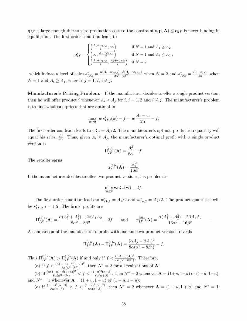
qIF is large enough due to zero production cost so the constraint s(p,A) ≤ qIF is never binding in

equilibrium. The first-order condition leads to

p∗IF =

(A1+wIF,1

2 ,∞)

if N = 1 and A1 ≥ A2(∞, A2+wIF,2

2

)if N = 1 and A1 ≤ A2(

A1+wIF,12 ,

A2+wIF,22

)if N = 2

,

which induce a level of sales s∗IF,i =α(Ai−wIF,i)−β(Aj−wIF,j)

2α2−2β2 when N = 2 and s∗IF,i =Ai−wIF,i

2α when

N = 1 and Ai ≥ Aj , where i, j = 1, 2, i 6= j.

Manufacturer’s Pricing Problem. If the manufacturer decides to offer a single product version,

then he will offer product i whenever Ai ≥ Aj for i, j = 1, 2 and i 6= j. The manufacturer’s problem

is to find wholesale prices that are optimal in

maxw≥0

w s∗IF,i(w)− f = wAi − w

2α− f.

The first order condition leads to w∗IF = Ai/2. The manufacturer’s optimal production quantity will

equal his sales, Ai4α . Thus, given Ai ≥ Aj , the manufacturer’s optimal profit with a single product

version is

Π(1)∗IF (A) =

A2i

8α− f.

The retailer earns

π(1)∗IF (A) =

A2i

16α.

If the manufacturer decides to offer two product versions, his problem is

maxw≥0

ws∗IF (w)− 2f.

The first order condition leads to w∗IF,1 = A1/2 and w∗IF,2 = A2/2. The product quantities will

be s∗IF,i, i = 1, 2. The firms’ profits are

Π(2)∗IF (A) =

α(A21 +A2

2)− 2βA1A2

8α2 − 8β2− 2f and π

(2)∗IF (A) =

α(A21 +A2

2)− 2βA1A2

16α2 − 16β2.

A comparison of the manufacturer’s profit with one and two product versions reveals

Π(2)∗IF (A)−Π

(1)∗IF (A) =

(αAj − βAi)2

8α(α2 − 8β2)− f.

Thus Π(2)∗IF (A) > Π

(1)∗IF (A) if and only if f <

(αAj−βAi)2

8α(α2−8β2). Therefore,

(a) if f < (α(1−u)−β(1+u))2

8α(α2−β2), then N∗ = 2 for all realizations of A;

(b) if (α(1−u)−β(1+u))2

8α(α2−β2)< f < (1−u)2(α−β)

8α(α+β) , then N∗ = 2 whenever A = (1+u, 1+u) or (1−u, 1−u),

and N∗ = 1 whenever A = (1 + u, 1− u) or (1− u, 1 + u);

(c) if (1−u)2(α−β)8α(α+β) < f < (1+u)2(α−β)

8α(α+β) , then N∗ = 2 whenever A = (1 + u, 1 + u) and N∗ = 1;

38

otherwise

(d) if (1+u)2(α−β)8α(α+β) < f , then N∗ ≤ 1 for all realizations of A.

The manufacturer’s expected profit E[Π(N)∗IF (A)] = E[max{Π(1)∗

IF (A),Π(2)∗IF (A2}] is

E[Π(N)∗IF (A)] =

α(1+u2)−8α2f−β+8β2f4(α2−β2) , if f ≤ (α(1−u)−β(1+u))2

8α(α2−β2)

α(3+2u+3u2−24βf)+β(1+u)2−24α2f16α(α+β) , if (α(1−u)−β(1+u))2

8α(α2−β2) < f ≤ (1−u)2(α−β)8α(α+β)

−40α2f+α(−40βf+5u2+6u+5)+β(3u2+2u+3)32α(α+β) , if (1−u)2(α−β)

8α(α+β) < f ≤ min{ (1+u)2(α−β)8α(α+β) , (1−u)2

8α }−16α2f+2α(−8βf+u2+2u+1)+β(u+1)2

16α(α+β) , if max{ (1−u)2(α−β)8α(α+β) , (1−u)2

8α } < f ≤ (1+u)2(α−β)8α(α+β)

−8αf+u2+u+18α , if (1+u)2(α−β)

8α(α+β) < f ≤ (1−u)2

8α

34

((u+1)2

8α − f), if max{ (1+u)2(α−β)

8α(α+β) , (1−u)2

8α } < f ≤ (1+u)2

8α

0, if f > (1+u)2

8α

.

The retailer’s corresponding expected profit is

E[π(N)∗IF (A)] =

α(1+u2)−β8(α2−β2) , if f ≤ (α(1−u)−β(1+u))2

8α(α2−β2)α(3u2+2u+3)+β(u+1)2

32α(α+β) , if (α(1−u)−β(1+u))2

8α(α2−β2) < f ≤ (1−u)2(α−β)8α(α+β)

α(5u2+6u+5)+β(3u2+2u+3)64α(α+β) , if (1−u)2(α−β)

8α(α+β) < f ≤ min{ (1+u)2(α−β)8α(α+β) , (1−u)2

8α }(u+1)2(2α+β)

32α(α+β) , if max{ (1−u)2(α−β)8α(α+β) , (1−u)2

8α } < f ≤ (1+u)2(α−β)8α(α+β)

1+u+u2

16α , if (1+u)2(α−β)8α(α+β) < f ≤ (1−u)2

8α

3(1+u)2

64α , if max{ (1+u)2(α−β)8α(α+β) , (1−u)2

8α } < f ≤ (1+u)2

8α

0, if f > (1+u)2

8α

.

We define πIF = E[π(N)∗IF (A)]. When π0 > πIF or f > (1+u)2

8α , IF is not feasible.

B.1 Proof of Proposition 3

We first derive the equilibrium outcome when N = 1 (we label this case using a mnemonic PH1);

then we obtain the equilibrium outcome when N = 2 (labeled PH2). Finally, we arrive at the result

in Proposition 3 by comparing profits across both cases.

B.1.1 PH1

Proof. The equilibrium is derived using backward induction.

Retail Pricing Decision. After demand is revealed, the retailer sets retail price so as to achieve

maxp≥0

p · s(p,A) s.t. s(p,A) ≤ qPH , (B.1)

which is equivalent to

max0≤s≤qPH

p(s,A) · s, (B.2)

39

where p(s,A) = A− αs. The optimal solution is given by

s∗PH = min

{A

2α, qPH

}and p∗PH = max

{A

2, A− αqPH

}.

Stocking Quantity Decision. Before demand is revealed, the retailer sets the stocking quantity

to achieve

maxqPH≥0

E[p∗PH · s∗PH ]− wPH · qPH ,

If qPH > 1+u2α , then s∗PH = A

2α for A = 1− u or 1 + u. Thus the retailer’s expected profit can be

simplified as 1+u2

4α − wPH · qPH , which is decreasing in qPH . Thus qPH > 1+u2 is not optimal.

If 1−u2α ≤ qPH ≤

1+u2α , then s∗PH = 1−u

2 when A = 1−u and s∗PH = qPH when A = 1+u. Thus the

retailer’s expected profit can be simplified as qPH(1+u−αqPH)2 + (1−u)2

8α − wPH · qPH . The first order

condition leads to qPH = 1+u−2wPH2α when wPH ≤ u.

If qPH < 1−u2α , then s∗PH = qPH when A = 1− u or 1 + u. Thus the retailer’s expected profit can

be simplified as qPH − αq2PH − wPH · qPH . The first order condition leads to qPH = 1−wPH

2α when

u < wPH ≤ 1. And when wPH > 1, qPH = 0. Thus the optimal stocking quantity is

q∗PH(wPH) =

1+u−2wPH

2α , if wPH ≤ u1−wPH

2α , if u < wPH ≤ 1

0, if wPH > 1

.

Wholesale Pricing Decision. As a function of wholesale price, the firms’ expected profits are

Π(1)PH(wPH) = −f +

1+u−2wPH

2α wPH , if wPH ≤ u1−wPH

2α wPH , if u < wPH ≤ 1

0, if wPH > 1

and

π(1)PH(wPH) =

u2−2uwPH+2w2

PH−2wPH+14α , if wPH ≤ u

(1−wPH)2

4α , if u < wPH ≤ 1

0, if wPH > 1

.

The manufacturer’s problem is set wholesale prices so as to achieve

maxwPH≥0

Π(1)PH (wPH) = wPH · q∗PH(wPH)− f (B.4a)

s.t. π(1)PH(wPH) ≥ π0, (B.4b)

where (B.4b) is the retailer’s participation constraint.

For any given π0, let w∗PL(π0), Π(1)∗PL (π0), and π

(1)∗PL (π0) denote the manufacturer’s optimal whole-

sale price, the manufacturer’s corresponding profit, and the retailer’s corresponding profit, respec-

tively. We first solve the unconstrained problem with π0 = 0. We just need to optimize Π(1)PH(wPH).

If wPH ≤ u, then the manufacturer’s profit can be simplified as Π(1)PH(wPH) = wPH

1+u−2wPH2α − f .

40

The first-order condition leads to wPH = 1+u4 if u > 1

3 , and the manufacturer’s corresponding

optimal profit is (1+u)2

16α . If u < wPH ≤ 1, then the manufacturer’s profit can be simplified as

Π(1)PH(wPH) = wPH

1−wPH2α − f . The first-order condition leads to wPH = 1

2 if u < 12 , and the manu-

facturer’s corresponding optimal profit is 18α . When 1

3 < u < 12 , both wPH = 1+u

4 and wPH = 12 are

the local optima. A comparison of the manufacturer’s profit at wPH = 1+u4 and wPH = 1

2 reveals

that wPH = 1+u4 is optimal when u >

√2− 1 and wPH = 1

2 is optimal when u <√

2− 1. Thus the

optimal wholesale price of the unconstrained problem (i.e., π0 = 0) is

w∗PH(0) =

1+u4 , if u ≥

√2− 1

12 , otherwise

.

The manufacturer’s and retailer’s corresponding profits are

Π(1)∗PH (0) = Π

(1)PH(w∗PH(0)) = −f +

(1+u)2

16α , if u ≥√

2− 1

18α , otherwise

and

π(1)∗PH (0) = π

(1)PH(w∗PH(0)) =

5−6u+5u2

32α , if u ≥√

2− 1

116α , otherwise

.

When π0 ≤ π(1)∗PH (0), the manufacturer faces the unconstrained problem and the solution is the

same as π0 = 0. When π0 > π(1)∗PH (0), in order to satisfy the retailer’s reservation constraint B.4b,

the manufacturer has to set wholesale price wPH < w∗PH(0) since the retailer’s profit decreases in

wPH . The manufacturer’s and retailer’s profits can be shown in Figure B.1. If u ≥√

2 − 1 or

u < 1/3 (see Figure B.1(a) and B.1(c)), then Π(1)PH(wPH) increases in wPH for wPH < w∗PH(0).

Thus, if π0 > π(1)∗PH (0), then the retailer’s reservation constraint (B.4b) will be active and the optimal

wholesale price will be solved from π(1)PH(wPH) = π0. If 1/3 < u <

√2 − 1 (see Figure B.1(b) ),

then Π(1)PH(wPH) first increases, then decreases, and then increases in wPH for wPH < w∗PH(0). We

define w(1)PH ∈ [u, 1/2] as Π

(1)PH(w

(1)PH) = Π

(1)PH(1+u

4 ). When π(1)PH(0) < π0 < π

(1)PH(w

(1)PH), the retailer’s

reservation constraint will be binding and the optimal wholesale price is solved from π(1)PH(wPH) = π0.

When π(1)PH(w

(1)PH) ≤ π0 ≤ π

(1)PH(1+u

4 ), the manufacturer’s optimal wholesale price is wPH = 1+u4 .

Finally, when π0 > π(1)PH(1+u

4 ), the retailer’s reservation constraint will again be binding.

Thus the optimal wholesale price is

w∗PH(π0) =

wPH,hv(π0), if u ≥√

2− 1

wPH,lv(π0), if u <

√2− 1

,

where

wPH,hv(π0) =

1+u

4 , if 0 ≤ π0 ≤ 5−6u+5u2

32α

1+u−√

8απ0−u2+2u−12 , if 5−6u+5u2

32α < π0 ≤ 1+u2

4α

0, if π0 > 1+u2

4α

41

Figure B.1: Firms’ Ex-ante Profit Function under PH1

(a) u ≥√

2− 1 and w∗PH(0) = 1+u4 (b) 1/3 ≤ u <

√2− 1 and w∗PH(0) = 1/2

(c) u < 1/3 and w∗PH(0) = 1/2

and

wPH,lv(π0) =

1/2, if 0 ≤ π0 ≤ 116α

1− 2√απ0, if 1

16α < π0 ≤

1−2u+u2

4α , if u ≤ 1/3√

2−4u−2u2

16α + 3−2u−u2

32α , if 1/3 < u <√

2− 1

1+u4 , if 1/3 < u <

√2− 1 and

√2−4u−2u2

16α + 3−2u−u2

32α ≤ π0 ≤ 5−6u+5u2

32α

1+u−√

8απ0−u2+2u−12 , if

1−2u+u2

4α , if u ≤ 1/3

5−6u+5u2

32α , if 1/3 < u <√

2− 1< π0 ≤ 1+u2

4α

0, if π0 > 1+u2

4α

.

The manufacturer’s and retailer’s corresponding profits are

42

(a) If u ≥√

2− 1, then

Π(1)∗PH (π0) = −f +

(1+u)2

16α , if 0 ≤ π0 ≤ 5−6u+5u2

32α√8απ0−u2+2u−1(1+u−

√8απ0−u2+2u−1)

4α , if 5−6u+5u2

32α < π0 ≤ 1+u2

4α

0, if π0 > 1+u2

4α

and

π(1)∗PH (π0) =

5−6u+5u2

32α , if 0 ≤ π0 ≤ 5−6u+5u2

32α

π0, if 5−6u+5u2

32α < π0 ≤ 1+u2

4α

0, if π0 > 1+u2

4α

.

(b) If u <√

2− 1, then

Π(1)∗PH (π0) = −f +

18α , if 0 ≤ π0 ≤ 1

16α√π0

α − 2π0, if 116α < π0 ≤

1−2u+u2

4α , if u ≤ 1/3√

2−4u−2u2

16α + 3−2u−u2

32α , if 1/3 < u <√

2− 1

(1+u)2

16α , if 1/3 < u <√

2− 1 and√

2−4u−2u2

16α + 3−2u−u2

32α ≤ π0 ≤ 5−6u+5u2

32α

X1, if

1−2u+u2

4α , if u ≤ 1/3

5−6u+5u2

32α , if 1/3 < u <√

2− 1< π0 ≤ 1+u2

4α

0, if π0 > 1+u2

4α

and

π(1)∗PH (π0) =

116α , if 0 ≤ π0 ≤ 1

16α

π0, if 116α < π0 ≤

1−2u+u2

4α , if u ≤ 1/3√

2−4u−2u2

16α + 3−2u−u2

32α , if 1/3 < u <√

2− 1

5−6u+5u2

32α , if 1/3 < u <√

2− 1 and√

2−4u−2u2

16α + 3−2u−u2

32α ≤ π0 ≤ 5−6u+5u2

32α

π0, if

1−2u+u2

4α , if u ≤ 1/3

5−6u+5u2

32α , if 1/3 < u <√

2− 1< π0 ≤ 1+u2

4α

0, if π0 > 1+u2

4α

,

where X1 =√

8απ0−u2+2u−1(1+u−√

8απ0−u2+2u−1)4α .

Π(1)∗PH (π0) decreases in π0 for 0 ≤ π0 ≤ 1+u2

4α . Thus there exists 0 ≤ πPH ≤ 1+u2

4α such that

Π(1)∗PH (π0) > 0 when π0 < πPH and Π

(1)∗PH (π0) < 0 when π0 > πPH . Therefore when π0 > πPH , PH1

is not feasible.

B.1.2 PH2

Proof. As in PH1, the equilibrium is derived using backward induction.

Retail Pricing Decision. After demand is revealed, the retailer sets retail prices so as to achieve

maxp≥0

p · s(p,A) s.t. s(p,A) ≤ qPH , (B.5)

43

which is equivalent to

max0≤s≤qPH

p(s,A) · s, (B.6)

where p(s,A) = (A1 − αs1 − βs2, A2 − αs2 − βs1). The optimal solution is given by

s∗PH,i = min

{qPH,i,max

{Ai − 2βqPH,j

2α,αAi − βAj2(α2 − β2)

}}and p∗PH,i = Ai − αs∗PH,i − βs∗PH,j ,

where i, j = 1, 2 and i 6= j.

Stocking Quantity Decision. Before demand is revealed, the retailer sets the stocking quantity

to achieve

maxqPH≥0

E[p∗PH · s∗PH ]−wPH · qPH .

We just need to focus on the symmetric solutions qPH,1 = qPH,2 when wPH,1 = wPH,2. This is due

to the following Lemma B.1.

Lemma B.1. If N = 2 and wPH,1 = wPH,2, then neither qPH,1 > qPH,2 > 0 nor 0 < qPH,1 < qPH,2

can be supported as an equilibrium with the PH contract.

Proof of Lemma B.1. Given wholesale prices wPH = (wPH,1, wPH,2) and qPH = (qPH,1, qPH,2), the

retailer’s profit can be written as π(2)PH(qPH) = E[p∗PH(qPH) · s∗PH(qPH)]−wPH · qPH . The retailer

chooses optimal qPH to maximize her expected profit.

We will show that given wPH,1 = wPH,2 = w(2)PH ≥ 0, any qPH,1 > qPH,2 > 0 is not optimal for

the retailer. We just need to show that there exists small enough 0 < δq < (qPH,1 − qPH,2)/2, such

that qPH = (qPH,1 − δq, qPH,2 + δq) dominates qPH , i.e., π(2)PH(qPH) > π

(2)PH(qPH).

Define RPH(qPH) = E[p∗PH(qPH) · s∗PH(qPH)]. Since π(2)PH(qPH) − π(2)

PH(qPH) = RPH(qPH) −RPH(qPH), we just need to show RPH(qPH) > RPH(qPH).

Taking the one-side derivative of RPH(qPH) with respective to qPH,1 and qPH,2, we have

∂RPH(qPH)

∂q−PH,1= lim

δq→0+

RPH(qPH,1 − δq, qPH,2)−RPH(qPH)

−δq> 0 and

∂RPH(qPH)

∂q+PH,2

= limδq→0+

RPH(qPH,1, qPH,2 + δq)−RPH(qPH)

δq> 0.

We can verify that ∂RPH(qPH)

∂q+PH,2

> ∂RPH(qPH)

∂q−PH,1

, that is the marginal value of increasing qPH,2 is

greater than that of qPH,1 for the retailer.

For small enough δq > 0, the Taylor series of RPH(qPH) can be written as

RPH(qPH) = RPH(qPH)− δq∂RPH(qPH)

∂q−PH,1+ δq

∂RPH(qPH)

∂q+PH,2

+ o(δq)

= RPH(qPH) + δq(∂RPH(qPH)

∂q+PH,2

− ∂RPH(qPH)

∂q−PH,1) + o(δq) > RPH(qPH).

Thus we have shown that for given wPH,1 = wPH,2 > 0, any qPH with qPH,1 > qPH,2 > 0 is not

44

optimal for the retailer. Similarly we can show that any qPH with 0 < qPH,1 < qPH,2 is not optimal

either. Thus the retailer’s optimal order quantities must satisfy qPH,1 = qPH,2.

We will now show that in the PH2 equilibrium, wPH,1 = wPH,2 holds in Lemma B.2.

Lemma B.2. If N = 2, then neither wPH,1 < wPH,2 nor wPH,1 > wPH,2 can be supported as an

equilibrium with the PH contract.

Proof of Lemma B.2. We show that given N = 2 under PH, any wPH = (wPH,1, wPH,2) with

wPH,1 < wPH,2 is not optimal for the manufacturer. We just need to show that there exist

0 ≤ δw1, δw2 < (wPH,2 − wPH,1)/2, such that wPH = (wPH,1 + δw1, wPH,2 − δw2) dominates wPH ,

i.e., Π(2)PH(wPH) > Π

(2)PH(wPH) and π

(2)PH(wPH) > π

(2)PH(wPH).

The manufacturer’s and retailer’s expected profits can be written as

Π(2)PH(wPH) = wPH · q∗PH(wPH)− 2f and

π(2)PH(wPH) = E[p∗PH(q∗PH(wPH)) · s∗PH(q∗PH(wPH))]−wPH · q∗PH(wPH).

For small enough δw1 and δw2, we have

Π(2)PH(wPH) = Π

(2)PH(wPH) + δw1

∂Π(2)PH(wPH)

∂w+PH,1

− δw2∂Π

(2)PH(wPH)

∂w−PH,2+ o(δw1) + o(δw2),

π(2)PH(wPH) = π

(2)PL(wPH) + δw1

∂π(2)PH(wPH)

∂w+PH,1

− δw2∂π

(2)PH(wPH)

∂w−PH,2+ o(δw1) + o(δw2).

To show Π(2)PH(wPH) > Π

(2)PL(wPH) and π

(2)PH(wPH) > π

(2)PH(wPH), we just need to show that

δw1∂Π

(2)PH(wPH)

∂w+PH,1

− δw2∂Π

(2)PH(wPH)

∂w−PH,2

> 0 and δw1∂π

(2)PH(wPH)

∂w+PH,1

− δw2∂π

(2)PH(wPH)

∂w−PH,2

> 0.

One can easily verify that∂π

(2)PH(wPH)

∂w+PH,1

<∂π

(2)PH(wPH)

∂w−PH,2

< 0, that is the retailer’s profit decreases

in the wholesale prices and is more sensitive to the lower wholesale price wPH,1 than the higher

wholesale price wPH,2.

If∂Π

(2)PH(wPH)

∂w−PH,2

< 0, then we just need to take δw1 = 0 and small enough δw2 > 0. Then we

have δw1∂Π

(2)PH(wPH)

∂w+PH,1

− δw2∂Π

(2)PH(wPH)

∂w−PH,2

= −δw2∂Π

(2)PH(wPH)

∂w−PH,2

> 0 and δw1∂π

(2)PH(wPH)

∂w+PH,1

− δw2∂π

(2)PH(wPH)

∂w−PH,2

=

−δw2∂π

(2)PH(wPH)

∂w−PH,2

> 0. Thus Π(2)PH(wPH) > Π

(2)PH(wPH) and π

(2)PH(wPH) > π

(2)PH(wPH).

If∂Π

(2)PH(wPH)

∂w−PH,2

≥ 0, then one can verify that∂Π

(2)PH(wPH)

∂w+PH,1

>∂Π

(2)PH(wPH)

∂w−PH,2

≥ 0, that is the manufac-

turer’s profit increases in the wholesale prices and is more sensitive to the lower wholesale price wPH,1

than the higher wholesale price wPH,2. And we can also show that 0 ≤ ∂Π(2)PH(wPH)

∂w−PH,2

/∂Π

(2)PH(wPH)

∂w+PH,1

<

∂π(2)PH(wPH)

∂w−PH,2

/∂π

(2)PH(wPH)

∂w+PH,1

. Therefore we can find small enough δw1 > 0 and δw2 > 0 that satisfy

45

∂Π(2)PH(wPH)

∂w−PH,2

/∂Π

(2)PH(wPH)

∂w+PH,1

< δw1δw2

<∂π

(2)PH(wPH)

∂w−PH,2

/∂π

(2)PH(wPH)

∂w+PH,1

, which will lead to

δw1∂Π

(2)PH(wPH)

∂w+PH,1

− δw2∂Π

(2)PH(wPH)

∂w−PH,2> 0 and δw1

∂π(2)PH(wPH)

∂w+PH,1

− δw2∂π

(2)PH(wPH)

∂w−PH,2> 0.

Therefore there exist wPH such that Π(2)PH(wPH) > Π

(2)PH(wPH) and π

(2)PH(wPH) > π

(2)PH(wPH). We

have shown that any wPH = (wPH,1, wPH,2) with wPH,1 < wPH,2 can not be supported as an equilibrium.

Similarly, we can show that any wPH = (wPH,1, wPH,2) with wPH,1 > wPH,2 can not be supported as an

equilibrium, either. Therefore, given N = 2 under PH, we must have wPH,1 = wPH,2 in an equilibrium.

Due to Lemma B.1 and B.2, we just need to consider the symmetric solutions. Let wPH,1 =

wPH,2 = w(2)PH and qPH,1 = qPH,2 = q

(2)PH .

If q(2)PH > α(1+u)−β(1−u)

2(α2−β2), then the retailer’s expected profit can be simplified as α+αu2−β

2(α2−β2)−

2w(2)PHq

(2)PH , which decreases in q

(2)PH . Thus q

(2)PH > α(1+u)−β(1−u)

2(α2−β2)is not optimal.

If 1+u2(α+β) < q

(2)PH ≤

α(1+u)−β(1−u)2(α2−β2)

, then the retailer’s expected profit can be written as

−4α3q(2)2PH + α

(4β2q

(2)2PH + u(8βq

(2)PH − 2) + 3u2 + 3

)+ 4α2q

(2)PH(−βq(2)PH + u+ 1) + β(2βq

(2)PH + u− 1)2

8α(α+ β)− 2w

(2)PHq

(2)PH .

The first order condition leads to q(2)PH =

α−β+αu+βu−4αw(2)PH

2α2−2β2 when w(2)PH ≤

uβ2α .

If 1−u2(α+β) ≤ q

(2)PH ≤

1+u2(α+β) , then the expected profit can be written as

−8α3q(2)2PH + 2α

(2βq

(2)PH + u(6βq

(2)PH − 2) + u2 + 1

)+ 4α2q

(2)PH(−3βq

(2)PH + 2u+ 2) + β(2βq

(2)PH + u− 1)2

8α(α+ β)− 2w

(2)PHq

(2)PH .

The first order condition leads to q(2)PH =

β(u−1)+2α(u−2w(2)PH+1)

4α2+2αβ−2β2 when uβ2α < w

(2)PH ≤ u.

If q(2)PH < 1−u

2(α+β) , then the retailer’s expected profit can be simplified as 2q(2)PH(1− qPH(α+ β))−

2w(2)PHq

(2)PH . The first order condition leads to q

(2)PH =

1−w(2)PH

2(α+β) when u < w(2)PH ≤ 1. And when w

(2)PH > 1,

q(2)PH = 0.

Given wPH,1 = wPH,2 = w(2)PH , the optimal stocking quantities are

q∗PH,1(wPH) = q∗PH,2(wPH) = q(2)∗PH (wPH) =

α−β+αu+βu−4αw(2)PH

2α2−2β2 , if w(2)PH ≤

uβ2α

β(u−1)+2α(u−2w(2)PH+1)

4α2+2αβ−2β2 , if uβ2α < w

(2)PH ≤ u

1−w(2)PH

2(α+β) , if u < w(2)PH ≤ 1

0, if w(2)PH > 1

.

Wholesale Pricing Decision. In this stage, the manufacturer chooses wholesale prices that are

optimal in

maxwPH≥0

Π(2)PH (wPH) = wPH · q∗PH(wPH)− 2f (B.7a)

46

s.t. π(2)PH(wPH) ≥ π0, (B.7b)

Above (B.7b) is the retailer’s participation constraint.

Using Lemma B.2, which implies wPH,1 = wPH,2 = w(2)PH , the manufacturer’s and retailer’s

expected profits are

Π(2)PH(w

(2)PH) = −2f +

α−β+αu+βu−4αw(2)PH

α2−β2 w(2)PH , if w

(2)PH ≤

uβ2α

β(u−1)+2α(u−2w(2)PH+1)

2α2+αβ−β2 w(2)PH , if uβ

2α < w(2)PH ≤ u

1−wPHα+β w

(2)PH , if u < w

(2)PH ≤ 1

0, if w(2)PH > 1

and

π(2)PH(w

(2)PH) =

α(u2−2uw

(2)PH+4w

(2)2PH −2w

(2)PH+1

)+β(2(1−u)w

(2)PH−1)

2(α2−β2), if w

(2)PH ≤

uβ2α

2α(u2−2uw

(2)PH+2w

(2)2PH −2w

(2)PH+1

)+β(1−u)(2w

(2)PH−u−1)

2(2α−β)(α+β) , if uβ2α < w

(2)PH ≤ u

(1−w(2)PH)2

2(α+β) , if u < w(2)PH ≤ 1

0, if wPH > 1

.

For any given π0, let w(2)∗PH (π0), Π

(2)∗PH (π0), and π

(2)∗PH (π0) denote the manufacturer’s optimal whole-

sale price, the manufacturer’s corresponding profit, and the retailer’s corresponding profit, respec-

tively. We first solve the unconstrained problem with π0 = 0. Similar to the analysis in PH1, we

just need to optimize Π(2)PH(w

(2)PH). The optimal wholesale price of the unconstrained problem is

w(2)∗PH (0) =

2α(1+u)−β(1−u)

8α , if u ≥ 2√

2−β+β−22+β

12 , otherwise

.

The manufacturer’s and retailer’s corresponding profits are

Π(2)∗PH (0) = Π

(2)PH(w

(2)∗PH (0)) = −2f +

(2α(u+1)+β(u−1))2

16α(2α−β)(α+β) , if u ≥ 2√

2−β+β−22+β

14(α+β) , otherwise

and

π(2)∗PH (0) = π

(2)PH(w

(2)∗PH (0)) =

4α2(5u2−6u+5)+4αβ(u2−1)−3β2(u−1)2

32α(2α−β)(α+β) , if u ≥ 2√

2−β+β−22+β

18(α+β) , otherwise

.

When π0 ≤ π(2)∗PH (0), the manufacturer faces the unconstrained problem and the solution is the same as

π0 = 0. When π0 > π(2)∗PH (0), in order to satisfy the retailer’s reservation constraint B.7b, the manufacturer

has to set wholesale price wPH < w(2)∗PH (0) since the retailer’s profit decreases in w

(2)PH . The manufacturer’s

and retailer’s profits can be shown in Figure B.2. If u ≥ 2√

2−β+β−22+β or u < 2−β

6−β (see Figure B.2(a) and

B.2(c)), then Π(2)PH(w

(2)PH) increases in w

(2)PH for w

(2)PH < w

(2)∗PH (0). Thus if π0 > π

(2)∗PH (0), then the retailer’s

reservation constraint (B.7b) will be active and the optimal wholesale price is solved from π(2)PH(w

(2)PH) = π0.

47

If 2−β6−β ≤ u < 2

√2−β+β−2

2+β (see Figure B.2(a)), then Π(2)PH(w

(2)PH) first increases, then decreases, and then

increases in w(2)PH for w

(2)PH < w

(2)∗PH (0). We define w

(2)PH ∈ [u, 1/2] as Π

(2)PH(w

(2)PH) = Π

(2)PH( 2(1+u)α−(1−u)β

8α ).

When π(2)PH(0) < π0 < π

(2)PH(w

(2)PH), the retailer’s reservation constraint will be binding. When π

(2)PH(w

(2)PH) <

π0 ≤ π(2)PH( 2(1+u)α−(1−u)β

8α ), the manufacturer’s optimal wholesale price will be w(2)PH = 2(1+u)α−(1−u)β

8α . And

when π0 > π(2)PH( 2(1+u)α−(1−u)β

8α ), the retailer’s reservation constraint will be binding again.

Figure B.2: Firms’ Ex-ante Profit Function under PH2

(a) u ≥ 2√

2−β+β−22+β and w

(2)∗PH (0) = wL (b) 2−β

6−β ≤ u <2√

2−β+β−22+β and w

(2)∗PH (0) = 1/2

(c) u < 2−β6−β and w

(2)∗PH (0) = 1/2

Note. wL = 2(1+u)α−(1−u)β8α .

Thus the optimal wholesale price is

w(2)∗PH (π0) =

w

(2)PH,hv(π

0), if u ≥ 2√

2−β+β−22+β

w(2)PH,mv(π

0), if 2−β6−β ≤ u <

2√

2−β+β−22+β

w(2)PH,lv(π

0), if u < 2−β6−β

,

48

where

w(2)PH,hv(π

0) =

2(1+u)α−(1−u)β8α , if π0 ≤ 4α2(5u2−6u+5)+4αβ(u2−1)−3β2(u−1)2

32α(2α−β)(α+β)12α(u+1)+ 1

4β(u−1)+ 14W2(β−2α)

α , if4α2(5u2−6u+5)+4αβ(u2−1)−3β2(u−1)2

32α(2α−β)(α+β) < π0 ≤ α+αu2−βu2α2+2αβ

α(u+1)+β(u+βW3α+β−1)−α

2W3α+β

4α , if α+αu2−βu2α2+2αβ < π0 ≤ α−β+αu2

2α2−2β2

0, if π0 > α−β+αu2

2α2−2β2

,

w(2)PH,mv(π

0) =

1/2, if π0 ≤ 18(α+β)

1−√

2(α+ β)π0, if 18(α+β) < π0 ≤W1

2(1+u)α−(1−u)β8α , if W1 < π0 ≤ 4α2(5u2−6u+5)+4αβ(u2−1)−3β2(u−1)2

32α(2α−β)(α+β)12α(u+1)+ 1

4β(u−1)+ 14W2(β−2α)

α , if4α2(5u2−6u+5)+4αβ(u2−1)−3β2(u−1)2

32α(2α−β)(α+β) < π0 ≤ α+αu2−βu2α2+2αβ

α(u+1)+β(u+βW3α+β−1)−α

2W3α+β

4α , if α+αu2−βu2α2+2αβ < π0 ≤ α−β+αu2

2α2−2β2

0, if π0 > α−β+αu2

2α2−2β2

,

and

w(2)PH,lv(π

0) =

1/2, if π0 ≤ 18(α+β)

1−√

2(α+ β)π0, if 18(α+β) < π0 ≤ 1+u2−2u

2(α+β)12α(u+1)+ 1

4β(u−1)+ 14W2(β−2α)

α , if 1+u2−2u2(α+β) < π0 ≤ α+αu2−βu

2α2+2αβ

α(u+1)+β(u+βW3α+β−1)−α

2W3α+β

4α , if α+αu2−βu2α2+2αβ < π0 ≤ α−β+αu2

2α2−2β2

0, if π0 > α−β+αu2

2α2−2β2

.

Above, we let W1 =

(√− (2α+β)(2α(u2+2u−1)+β(u−1)2)

α(2α−β) +2

)2

32(α+β) , W2 =√

8α2π0−2α(−4βπ0+u2−2u+1)−β(u−1)2

2α−β , and

W3 =√

8α2π0+α(8βπ0−3u2+2u−3)−β(u−1)2

α−β .

The manufacturer’s and retailer’s corresponding profits are

(a) If u ≥ 2√

2−β+β−22+β , then

Π(2)∗PH (π0) = −2f +

(2α(u+1)+β(u−1))2

16α(2α−β)(α+β) , if π0 ≤ 4α2(5u2−6u+5)+4αβ(u2−1)−3β2(u−1)2

32α(2α−β)(α+β)

−S1(β+S1

√2α−β−2α(u+1)−βu)

4α√

2α−β(α+β), if

4α2(5u2−6u+5)+4αβ(u2−1)−3β2(u−1)2

32α(2α−β)(α+β) < π0 ≤ α+αu2−βu2α2+2αβ

−S2(β+S2(α−β)+α(−u−1)−βu)4α(α+β) , if α+αu2−βu

2α2+2αβ < π0 ≤ α−β+αu2

2α2−2β2

0, if π0 > α−β+αu2

2α2−2β2

and

π(2)∗PH (π0) =

4α2(5u2−6u+5)+4αβ(u2−1)−3β2(u−1)2

32α(2α−β)(α+β) , if π0 ≤ 4α2(5u2−6u+5)+4αβ(u2−1)−3β2(u−1)2

32α(2α−β)(α+β)

π0, if4α2(5u2−6u+5)+4αβ(u2−1)−3β2(u−1)2

32α(2α−β)(α+β) < π0 ≤ α−β+αu2

2α2−2β2

0, if π0 > α−β+αu2

2α2−2β2

.

(b) If 2−β6−β ≤ u <

2√

2−β+β−22+β , then

49

Π(2)∗PH (π0) = −2f +

14(α+β) , if π0 ≤ 1

8(α+β)√2π0

α+β − 2π0, if 18(α+β) < π0 ≤W1

(2α(u+1)+β(u−1))2

16α(2α−β)(α+β) , if W1 < π0 ≤ 4α2(5u2−6u+5)+4αβ(u2−1)−3β2(u−1)2

32α(2α−β)(α+β)

−S1(β+S1

√2α−β−2α(u+1)−βu)

4α√

2α−β(α+β), if

4α2(5u2−6u+5)+4αβ(u2−1)−3β2(u−1)2

32α(2α−β)(α+β) < π0 ≤ α+αu2−βu2α2+2αβ

−S2(β+S2(α−β)+α(−u−1)−βu)4α(α+β) , if α+αu2−βu

2α2+2αβ < π0 ≤ α−β+αu2

2α2−2β2

0, if π0 > α−β+αu2

2α2−2β2

and

π(2)∗PH (π0) =

18(α+β) , if π0 ≤ 1

8(α+β)

π0, if 18(α+β) < π0 ≤W1

4α2(5u2−6u+5)+4αβ(u2−1)−3β2(u−1)2

32α(2α−β)(α+β) , if W1 < π0 ≤ 4α2(5u2−6u+5)+4αβ(u2−1)−3β2(u−1)2

32α(2α−β)(α+β)

π0, if4α2(5u2−6u+5)+4αβ(u2−1)−3β2(u−1)2

32α(2α−β)(α+β) < π0 ≤ α−β+αu2

2α2−2β2

0, if π0 > α−β+αu2

2α2−2β2

.

(c) If u < 2−β6−β , then

Π(2)∗PH (π0) = −2f +

14(α+β) , if π0 ≤ 1

8(α+β)√2π0

α+β − 2π0, if 18(α+β)π

0 ≤ 1+u2−2u2(α+β)

−S1(β+S1

√2α−β−2α(u+1)−βu)

4α√

2α−β(α+β), if 1+u2−2u

2(α+β) < π0 ≤ α+αu2−βu2α2+2αβ

−S2(β+S2(α−β)+α(−u−1)−βu)4α(α+β) , if α+αu2−βu

2α2+2αβ < π0 ≤ α−β+αu2

2α2−2β2

0, if π0 > α−β+αu2

2α2−2β2

,

π(2)∗PH (π0) =

1

8(α+β) , if π0 ≤ 18(α+β)

π0, if 18(α+β) < π0 ≤ α−β+αu2

2α2−2β2

0, if π0 > α−β+αu2

2α2−2β2

where S1 =√

8α2π0 − 2α (−4βπ0 + u2 − 2u+ 1)− β(u− 1)2 and S2 =√

8α2π0+α(8βπ0−3u2+2u−3)−β(u−1)2

α−β .

Π(2)∗PH (π0) decreases in π0 for 0 ≤ π0 ≤ α−β+αu2

2α2−2β2 . Thus there exists 0 ≤ π(2)PH ≤

α−β+αu2

2α2−2β2 such that

Π(2)∗PH (π0) > 0 when π0 < π

(2)PH and Π

(2)∗PH (π0) < 0 when π0 > π

(2)PH . Therefore when π0 > π

(2)PH , PH2 is not

feasible.

B.1.3 PH1 vs. PH2

Proof. Now, we compare profits to determine when PH1 and PH2 should be expected in equilibrium.

To do this, one can check that Π(2)∗PH (π0) is decreasing in β and Π

(1)∗PH (π0) is independent in β.

(a) If Π(2)∗PH (π0) > max{Π(1)∗

PH (π0), 0} for any β ∈ [0, α1−u1+u ], then let βPH(π0) = α1−u

1+u .

(b) If Π(2)∗PH (π0) < max{Π(1)∗

PH (π0), 0} for any β ∈ [0, α1−u1+u ], then let βPH(π0) = 0.

50

(c) Otherwise there exists βPH(π0) ∈ [0, α1−u1+u ] such that Π

(2)∗PH (π0) > max{Π(1)∗

PH (π0), 0} whenever

β < βPH(π0), Π(2)∗PH (π0) < max{Π(1)∗

PH (π0), 0}, and β > βPH(π0).

Thus if β < βPH(π0), then N∗ = 2 under PH. If β > βPH(π0), then N∗ = 1 whenever π0 ≤ πPH ;

and N∗ = 0 whenever π0 > πPH since N = 1 under PH is not feasible. This completes the proof of

Proposition 3.

C Proof of Proposition 4

Proof. From Proposition 1, we can see that in the centralized supply chain, when f > (α(1−u)−β(1+u))2

4α(α2−β2),

the manufacturer will not sell two product versions if the realized market potential is A = (1+u, 1−u)

or (1− u, 1 + u).

From the proof of Proposition 3, one can check that under PH contract,d(Π

(2)∗PH (π0)−max{Π(1)∗

PH (π0),0})df <

0, that is the manufacturer’s profit difference under PH2 and PH1 is decreasing in f . For any given

β ∈ [0, α1−u1+u ] and π0 ∈ [0, π

(2)PH ], we have Π

(2)∗PH (π0) − max{Π(1)∗

PH (π0), 0} ≥ 0 for f = 0. Therefore,

there exists fPH(β, π0) ≥ 0 such that Π(2)∗PH (π0)−max{Π(1)∗

PH (π0), 0} ≥ 0 for f ≤ fPH(β, π0), that it

the manufacturer will be optimal to produce two product version under PH.

Therefore, when (α(1−u)−β(1+u))2

4α(α2−β2)< f < fPH(β, π0), the manufacturer will always sell two product

versions under PH, but will sell less than two product versions in the centralized supply chain if the

realized market potential is A = (1 + u, 1− u) or (1− u, 1 + u).

D Proof of Corollary 1

Proof. From the proof of Proposition 3, one can check that∂Π

(1)∗PH (π0)

∂π0 < 0,∂Π

(1)∗PH (π0)∂f < 0 and

∂Π(1)∗PH (π0)∂u > 0. πPH is defined as Π

(1)∗PH (πPH) = 0. Thus ∂πPH

∂f = −∂Π(1)∗PH (π0)∂f

/∂Π

(1)∗PH (π0)

∂π0 < 0 and

∂πPH∂u = −∂Π

(1)∗PH (π0)∂u

/∂Π

(1)∗PH (π0)

∂π0 > 0. Therefore πPH decreases in f and increases in u.

βPH(π0) is defined as Π(2)∗PH (π0) = max{Π(1)∗

PH (π0), 0} for β = βPH(π0). When π0 > πPH , PH1

is not feasible and thus Π(2)∗PH (π0) = 0 for β = βPH(π0). One can check that Π

(2)∗PH (π0) decreases

in β and π0, and increases in u. Thus ∂βPH(π0)∂π0 = −∂Π

(2)∗PH (π0)

∂π0

/∂Π

(2)∗PH (π0)∂β < 0 and ∂βPH(π0)

∂u =

−dΠ(2)∗PH (π0)∂u

/∂Π

(2)∗PH (π0)∂β > 0, that is βPH(π0) decreases in π0 and increases in u.

When π0 ≤ πPH , PH1 is feasible and βPH(π0) is defined as Π(2)∗PH (π0) = Π

(1)∗PH (π0) for β =

βPH(π0). We can verify that∂(Π

(2)∗PH (π0)−Π

(1)∗PH (π0))

∂β < 0 and∂(Π

(2)∗PH (π0)−Π

(1)∗PH (π0))

∂π0 > 0 if u >√

2 − 1.

Thus if u >√

2−1, then ∂βPH(π0)∂π0 = −∂(Π

(2)∗PH (π0)−Π

(1)∗PH (π0))

∂π0

/∂(Π

(2)∗PH (π0)−Π

(1)∗PH (π0))

∂β > 0, that is βPH(π0)

increases in π0.

At last, one can verify that Π(2)∗PH (π0) −max{Π(1)∗

PH (π0), 0} decreases in β and f . Thus we have

∂βPH(π0)∂f = −∂(Π

(2)∗PH (π0)−max{Π(1)∗

PH (π0),0})∂f

/∂(Π

(2)∗PH (π0)−max{Π(1)∗

PH (π0),0})∂β > 0, that is βPH(π0) decreases

in f .

51

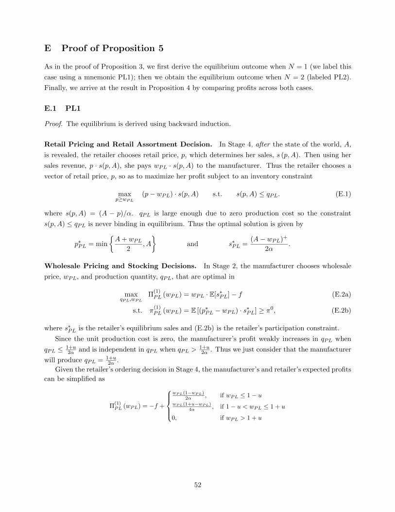
E Proof of Proposition 5

As in the proof of Proposition 3, we first derive the equilibrium outcome when N = 1 (we label this

case using a mnemonic PL1); then we obtain the equilibrium outcome when N = 2 (labeled PL2).

Finally, we arrive at the result in Proposition 4 by comparing profits across both cases.

E.1 PL1

Proof. The equilibrium is derived using backward induction.

Retail Pricing and Retail Assortment Decision. In Stage 4, after the state of the world, A,

is revealed, the retailer chooses retail price, p, which determines her sales, s (p,A). Then using her

sales revenue, p · s(p,A), she pays wPL · s(p,A) to the manufacturer. Thus the retailer chooses a

vector of retail price, p, so as to maximize her profit subject to an inventory constraint

maxp≥wPL

(p− wPL) · s(p,A) s.t. s(p,A) ≤ qPL. (E.1)

where s(p,A) = (A − p)/α. qPL is large enough due to zero production cost so the constraint

s(p,A) ≤ qPL is never binding in equilibrium. Thus the optimal solution is given by

p∗PL = min

{A+ wPL

2, A

}and s∗PL =

(A− wPL)+

2α.

Wholesale Pricing and Stocking Decisions. In Stage 2, the manufacturer chooses wholesale

price, wPL, and production quantity, qPL, that are optimal in

maxqPL,wPL

Π(1)PL (wPL) = wPL · E[s∗PL]− f (E.2a)

s.t. π(1)PL (wPL) = E [(p∗PL − wPL) · s∗PL] ≥ π0, (E.2b)

where s∗PL is the retailer’s equilibrium sales and (E.2b) is the retailer’s participation constraint.

Since the unit production cost is zero, the manufacturer’s profit weakly increases in qPL when

qPL ≤ 1+u2α and is independent in qPL when qPL >

1+u2α . Thus we just consider that the manufacturer

will produce qPL = 1+u2α .

Given the retailer’s ordering decision in Stage 4, the manufacturer’s and retailer’s expected profits

can be simplified as

Π(1)PL (wPL) = −f +

wPL(1−wPL)

2α , if wPL ≤ 1− uwPL(1+u−wPL)

4α , if 1− u < wPL ≤ 1 + u

0, if wPL > 1 + u

52

and

π(1)PL (wPL) =

u2+(1−wPL)2

4α , if wPL ≤ 1− u(1+u−wPL)2

8α , if 1− u < wPL ≤ 1 + u

0, if wPL > 1 + u

.

For any given π0, let w∗PL(π0), Π(1)∗PL (π0), and π

(1)∗PL (π0) denote the manufacturer’s optimal whole-

sale price, the manufacturer’s corresponding profit, and the retailer’s corresponding profit, respec-

tively. We first solve the unconstrained problem where π0 = 0. We just need to optimize Π(1)PL(wPL)

and the optimal wholesale price is

w∗PL(0) =

1/2, if u ≤√

2− 1

(1 + u)/2, if u >√

2− 1.

The manufacturer’s and retailer’s corresponding profits are

Π(1)∗PL (0) = Π

(1)PL(w∗PL(0)) = −f +

18α , if u ≤

√2− 1

(1+u)2

16α , if u >√

2− 1

and

π(1)∗PL (0) = π

(1)PL(w∗PL(0)) =

1+4u2

16α , if u ≤√

2− 1

(1+u)2

32α , if u >√

2− 1.

When π0 ≤ π(1)∗PL (0), the manufacturer faces the unconstrained problem and the solution is the

same as π0 = 0. When π0 > π(1)∗PL (0), in order to satisfy the retailer’s reservation constraint E.2b,

the manufacturer has to set the wholesale price wPL < w∗PL(0) since the retailer’s profit decreases

in wPL. The manufacturer’s and retailer’s expected profits are shown in Figure E.1. If u ≥ 1/2 or

u <√

2 − 1 (see Figure E.1(a) and E.1(c)), then Π(1)PL(wPL) increases in wPL for wPL < w∗PL(0).

Thus if π0 > π(1)∗PL (0), then the retailer’s reservation constraint (E.2b) will be active and the optimal

solution is solved from π(1)PL(wPL) = π0. If

√2−1 ≤ u < 1/2 (see Figure E.1(b)), then Π

(1)PL(wPL) first

increases, then decreases, and then increases in wPL for wPL < w∗PL(0). We define w(1)PL ∈ [1−u, 1+u

2 ]

as Π(1)PL(w

(1)PL) = Π

(1)PL(1/2). When π

(1)PL(0) < π0 < π

(1)PL(w

(1)PL), the retailer’s reservation constraint

will be binding. When π(1)PL(w

(1)PL) < π0 ≤ π(1)

PL(1/2), the manufacturer’s optimal wholesale price will

be wPL = 1/2. And when π0 > π(1)PL(1/2), the retailer’s reservation constraint will be binding again.

Thus the optimal wholesale price is

w∗PL(π0) =

wPL,hv(π0), if u >√

2− 1

wPL,lv(π0), if u ≤

√2− 1

,

53

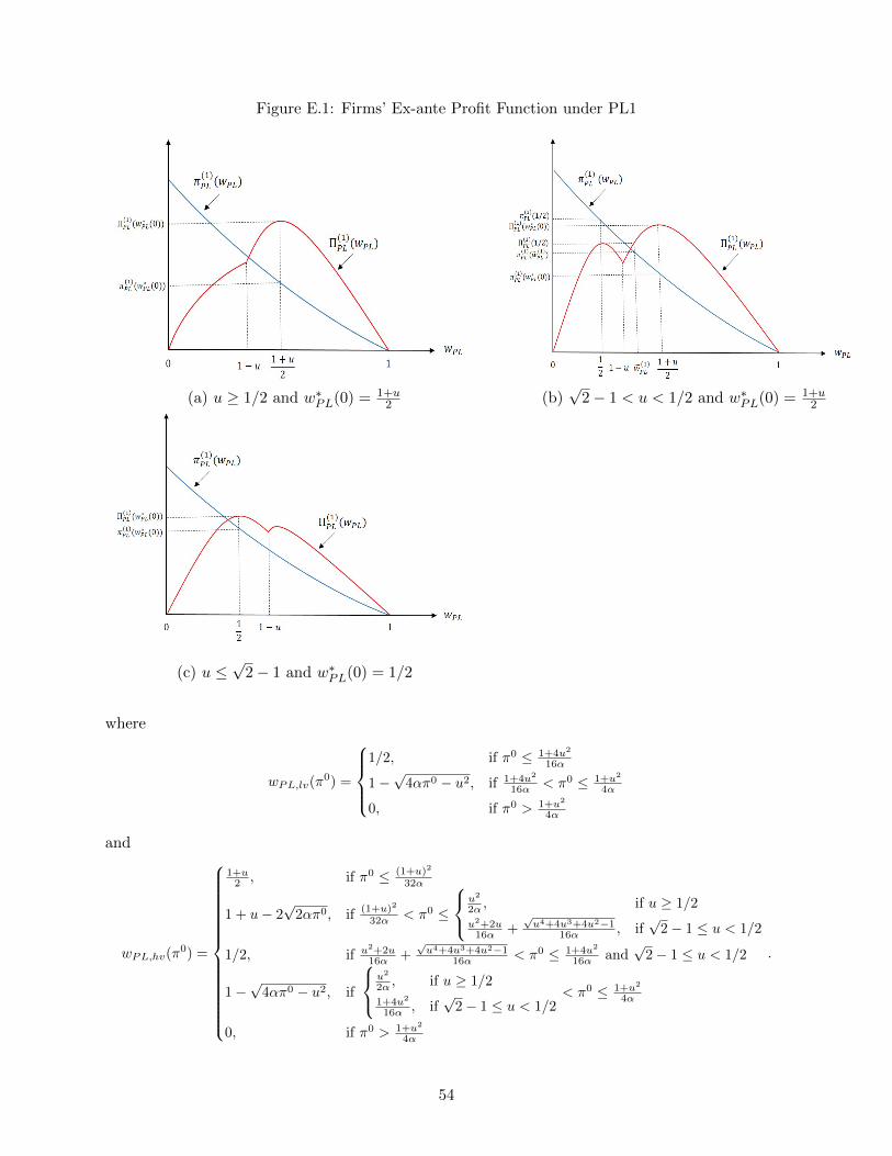
Figure E.1: Firms’ Ex-ante Profit Function under PL1

(a) u ≥ 1/2 and w∗PL(0) = 1+u2 (b)

√2− 1 < u < 1/2 and w∗PL(0) = 1+u

2

(c) u ≤√

2− 1 and w∗PL(0) = 1/2

where

wPL,lv(π0) =

1/2, if π0 ≤ 1+4u2

16α

1−√

4απ0 − u2, if 1+4u2

16α < π0 ≤ 1+u2

4α

0, if π0 > 1+u2

4α

and

wPL,hv(π0) =

1+u2 , if π0 ≤ (1+u)2

32α

1 + u− 2√

2απ0, if (1+u)2

32α < π0 ≤

u2

2α , if u ≥ 1/2

u2+2u16α +

√u4+4u3+4u2−1

16α , if√

2− 1 ≤ u < 1/2

1/2, if u2+2u16α +

√u4+4u3+4u2−1

16α < π0 ≤ 1+4u2

16α and√

2− 1 ≤ u < 1/2

1−√

4απ0 − u2, if

u2

2α , if u ≥ 1/2

1+4u2

16α , if√

2− 1 ≤ u < 1/2< π0 ≤ 1+u2

4α

0, if π0 > 1+u2

4α

.

54

The manufacturer’s and retailer’s corresponding profits are as follows

(a) If u >√

2− 1, then

Π(1)∗PL (π0) = −f +

(1+u)2

16α , if π0 ≤ (1+u)2

32α

√π0(u+1)−2

√2απ0

√2α

, if (1+u)2

32α < π0 ≤

u2

2α , if u ≥ 1/2

u2+2u16α +

√u4+4u3+4u2−1

16α , if√

2− 1 ≤ u < 1/2

18α , if u2+2u

16α +√u4+4u3+4u2−1

16α < π0 ≤ 1+4u2

16α and√

2− 1 ≤ u < 1/2

−4απ0+√

4απ0−u2+u2

2α , if

u2

2α , if u ≥ 1/2

1+4u2

16α , if√

2− 1 ≤ u < 1/2< π0 ≤ 1+u2

4α

0, if π0 > 1+u2

4α

and

π(1)∗PL (π0) =

(1+u)2

32α , if π0 ≤ (1+u)2

32α

π0, if (1+u)2

32α < π0 ≤

u2

2α , if u ≥ 1/2

1+4u2

16α , if√

2− 1 ≤ u < 1/2

1+4u2

16α , if u2+2u16α +

√u4+4u3+4u2−1

16α < π0 ≤ 1+4u2

16α and√

2− 1 ≤ u < 1/2

π0, if

u2

2α , if u ≥ 1/2

1+4u2

16α , if√

2− 1 ≤ u < 1/2< π0 ≤ 1+u2

4α

0, if π0 > 1+u2

4α

.

(b) If u ≤√

2− 1, then

Π(1)∗PL (π0) = −f +

1

8α , if π0 ≤ 1+4u2

16α

−4απ0+√

4απ0−u2+u2

2α , if 1+4u2

16α < π0 ≤ 1+u2

4α

0, if π0 > 1+u2

4α ,

and

π(1)∗PL (π0) =

1+4u2

16α , if π0 ≤ 1+4u2

16α

π0, if 1+4u2

16α < π0 ≤ 1+u2

4α

0, if π0 > 1+u2

4α

.

Π(1)∗PL (π0) decreases in π0 for 0 ≤ π0 ≤ 1+u2

4α . Thus there exists 0 ≤ πPL ≤ 1+u2

4α such that Π(1)∗PL (π0) >

0 when π0 < πPL and Π(1)∗PL (π0) < 0 when π0 > πPL. Thus PL1 is not feasible when π0 > πPL.

E.2 PL2

Proof. As before, the equilibrium is derived using backward induction.

55

Retail Pricing and Retail Assortment Decision. In Stage 4, after the state of the world, A,

is revealed, the retailer chooses a vector of retail prices, p, which determine her sales, s (p,A). Then

using her sales revenue, p · s(p,A), she pays wPL · s(p,A) to the manufacturer. As such, the retailer

chooses a vector of retail prices, p, so as to maximize her profit subject to an inventory constraint

maxp≥wPL

(p−wPL) · s(p,A) s.t. s(p,A) ≤ qPL. (E.3)

As in PL1, qPL is large enough so that the quantity constraint is never binding. Thus the optimal

solution is given by

s∗PL,i =

α(Ai−wi)−β(Aj−wj)

2(α2−β2), if wi < Ai and β

α(Aj − wj) < Ai − wi < αβ (Aj − wj)

Ai−wi2α , if Ai − wi ≥ α

β (Aj − wj)

0, otherwise ,

and

p∗PL,i = Ai − αs∗PL,i − βs∗PL,j , for i, j = 1, 2, i 6= j.

Wholesale Pricing and Stocking Decisions. In Stage 2, the manufacturer chooses wholesale

prices, wPL, and production quantities, qPL, that are optimal in

maxqPL,wPl

Π(2)PL (wPL) = wPL · E[s∗PL]− 2f (E.4a)

s.t. π(2)PL (wPL) = E [(p∗PL −wPL) · s∗PL] ≥ π0, (E.4b)

where s∗PL is the retailer’s equilibrium sales and (E.4b) is the retailer’s participation constraint.

Since the unit production cost is zero, the manufacturer’s profit weakly increases in qPL when

qPL ≤ (1+u2α ,

1+u2α ) and is independent in qPL when qPL > (1+u

2α ,1+u2α ). Thus we just consider the

manufacturer will produce qPL = (1+u2α ,

1+u2α ).

The following lemma shows that under PL2, we must have wPL,1 = wPL,2 in equilibrium.

Lemma E.1. If N = 2, then neither wPL,1 < wPL,2 nor wPL,1 > wPL,2 can be supported as an

equilibrium with the PL contract.

Proof of Lemma E.1. We show that given N = 2 under PL, any wPL = (wPL,1, wPL,2) with wPL,1 <

wPL,2 is not optimal for the manufacturer. We just need to show that there exist 0 ≤ δw1, δw2 <

(wPL,2 −wPL,1)/2, such that wPL = (wPL,1 + δw1, wPL,2 − δw2) dominates wPL, i.e., Π(2)PL(wPL) >

Π(2)PL(wPL) and π

(2)PL(wPL) > π

(2)PL(wPL).

The manufacturer’s and retailer’s expected profits can be written as

Π(2)PL(wPL) = wPL · E[s∗PL(wPL)]− 2f and

π(2)PL(wPL) = E[(pPL(s∗PL(wPL))−wPL) · s∗PL(wPL)].

For small enough δw1 and δw2, we have

56

Π(2)PL(wPL) = Π

(2)PL(wPL) + δw1

∂Π(2)PL(wPL)

∂w+PL,1

− δw2∂Π

(2)PL(wPL)

∂w−PL,2+ o(δw1) + o(δw2) and

π(2)PL(wPL) = π

(2)PL(wPL) + δw1

∂π(2)PL(wPL)

∂w+PL,1

− δw2∂π

(2)PL(wPL)

∂w−PL,2+ o(δw1) + o(δw2).

To show Π(2)PL(wPL) > Π

(2)PL(wPL) and π

(2)PL(wPL) > π

(2)PL(wPL), we just need to show that

δw1∂Π

(2)PL(wPL)

∂w+PL,1

− δw2∂Π

(2)PL(wPL)

∂w−PL,2

> 0 and δw1∂π

(2)PL(wPL)

∂w+PL,1

− δw2∂π

(2)PL(wPL)

∂w−PL,2

> 0.

One can easily verify that∂π

(2)PL(wPL)

∂w+PL,1

<∂π

(2)PL(wPL)

∂w−PL,2

< 0, that is the retailer’s profit decreases in the

wholesale prices and is more sensitive to the lower wholesale price wPL,1 than the higher wholesale

price wPL,2.

If∂Π

(2)PL(wPL)

∂w−PL,2

< 0, then we just need to take δw1 = 0 and small enough δw2 > 0. Then we

have δw1∂Π

(2)PL(wPL)

∂w+PL,1

− δw2∂Π

(2)PL(wPL)

∂w−PL,2

= −δw2∂Π

(2)PL(wPL)

∂w−PL,2

> 0 and δw1∂π

(2)PL(wPL)

∂w+PL,1

− δw2∂π

(2)PL(wPL)

∂w−PL,2

=

−δw2∂π

(2)PL(wPL)

∂w−PL,2

> 0. Thus Π(2)PL(wPL) > Π

(2)PL(wPL) and π

(2)PL(wPL) > π

(2)PL(wPL).

If∂Π

(2)PL(wPL)

∂w−PL,2

≥ 0, then one can verify that∂Π

(2)PL(wPL)

∂w+PL,1

>∂Π

(2)PL(wPL)

∂w−PL,2

≥ 0, that is the manufac-

turer’s profit increases in the wholesale prices and is more sensitive to the lower wholesale price

wPL,1 than the higher wholesale price wPL,2. We can also verify that 0 ≤ ∂Π(2)PL(wPL)

∂w−PL,2

/∂Π

(2)PL(wPL)

∂w+PL,1

<

∂π(2)PL(wPL)

∂w−PL,2

/∂π

(2)PL(wPL)

∂w+PL,1

. Therefore we can find small enough δw1 > 0 and δw2 > 0 that satisfy

∂Π(2)PL(wPL)

∂w−PL,2

/∂Π

(2)PL(wPL)

∂w+PL,1

< δw1δw2

<∂π

(2)PL(wPL)

∂w−PL,2

/∂π

(2)PL(wPL)

∂w+PL,1

, which leads to

δw1∂Π

(2)PL(wPL)

∂w+PL,1

− δw2∂Π

(2)PL(wPL)

∂w−PL,2> 0 and δw1

∂π(2)PL(wPL)

∂w+PL,1

− δw2∂π

(2)PL(wPL)

∂w−PL,2> 0.

Therefore Π(2)PL(wPL) > Π

(2)PL(wPL) and π

(2)PL(wPL) > π

(2)PL(wPL). We have shown that any

wPL = (wPL,1, wPL,2) with wPL,1 < wPL,2 can not be supported as an equilibrium. Similarly, we

can show that any wPL = (wPL,1, wPL,2) with wPL,1 > wPL,2 can not be supported as an equilibrium,

either. Therefore, given N = 2 under PL, we must have wPL,1 = wPL,2 in an equilibrium.

Due to Lemma E.1, we just need to consider wPL,1 = wPL,2 = w(2)PL. Given the retailer’s ordering

decision in Stage 4, the manufacturer’s and retailer’s expected profits can therefore be simplified as

Π(2)PL

(w

(2)PL

)= −2f +

w(2)PL

1−w(2)PL

α+β , if w(2)PL ≤

α(1−u)−β(1+u)α−β

w(2)PL

α(3+u−3w(2)PL)+β(1+u−w(2)

PL)

4α(α+β) , if α(1−u)−β(1+u)α−β < w

(2)PL ≤ 1− u

w(2)PL

(2α+β)(1+u−w(2)PL)

4α(α+β) , if 1− u < w(2)PL ≤ 1 + u

0, if w(2)PL > 1 + u

57

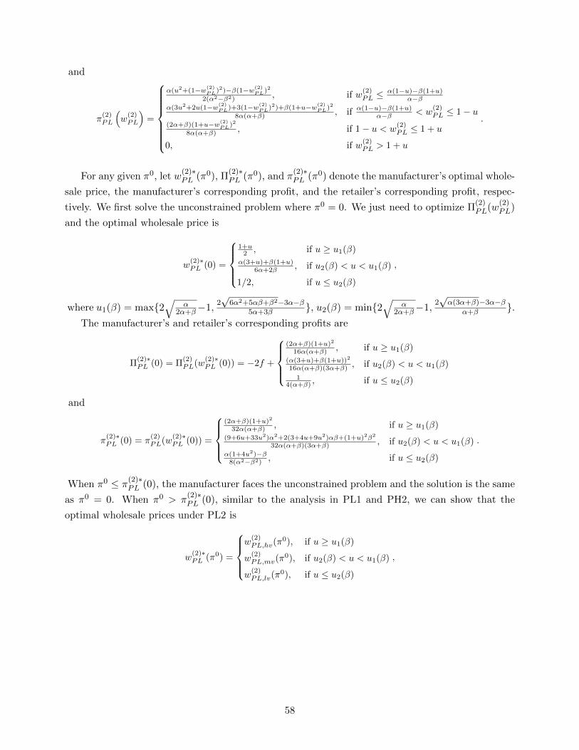
and

π(2)PL

(w

(2)PL

)=

α(u2+(1−w(2)PL)2)−β(1−w(2)

PL)2

2(α2−β2) , if w(2)PL ≤

α(1−u)−β(1+u)α−β

α(3u2+2u(1−w(2)PL)+3(1−w(2)

PL)2)+β(1+u−w(2)PL)2

8α(α+β) , if α(1−u)−β(1+u)α−β < w

(2)PL ≤ 1− u

(2α+β)(1+u−w(2)PL)2

8α(α+β) , if 1− u < w(2)PL ≤ 1 + u

0, if w(2)PL > 1 + u

.

For any given π0, let w(2)∗PL (π0), Π

(2)∗PL (π0), and π

(2)∗PL (π0) denote the manufacturer’s optimal whole-

sale price, the manufacturer’s corresponding profit, and the retailer’s corresponding profit, respec-

tively. We first solve the unconstrained problem where π0 = 0. We just need to optimize Π(2)PL(w

(2)PL)

and the optimal wholesale price is

w(2)∗PL (0) =

1+u

2 , if u ≥ u1(β)

α(3+u)+β(1+u)6α+2β , if u2(β) < u < u1(β)

1/2, if u ≤ u2(β)

,

where u1(β) = max{2√

α2α+β−1,

2√

6α2+5αβ+β2−3α−β5α+3β }, u2(β) = min{2

√α

2α+β−1,2√α(3α+β)−3α−β

α+β }.The manufacturer’s and retailer’s corresponding profits are

Π(2)∗PL (0) = Π

(2)PL(w

(2)∗PL (0)) = −2f +

(2α+β)(1+u)2

16α(α+β) , if u ≥ u1(β)

(α(3+u)+β(1+u))2

16α(α+β)(3α+β) , if u2(β) < u < u1(β)

14(α+β) , if u ≤ u2(β)

and

π(2)∗PL (0) = π

(2)PL(w

(2)∗PL (0)) =

(2α+β)(1+u)2

32α(α+β) , if u ≥ u1(β)

(9+6u+33u2)α2+2(3+4u+9u2)αβ+(1+u)2β2

32α(α+β)(3α+β) , if u2(β) < u < u1(β)

α(1+4u2)−β8(α2−β2) , if u ≤ u2(β)

.

When π0 ≤ π(2)∗PL (0), the manufacturer faces the unconstrained problem and the solution is the same

as π0 = 0. When π0 > π(2)∗PL (0), similar to the analysis in PL1 and PH2, we can show that the

optimal wholesale prices under PL2 is

w(2)∗PL (π0) =

w

(2)PL,hv(π

0), if u ≥ u1(β)

w(2)PL,mv(π

0), if u2(β) < u < u1(β)

w(2)PL,lv(π

0), if u ≤ u2(β)

,

58

where

w(2)PL,hv(π

0) =

1+u2 , if π0 ≤ (2α+β)(1+u)2

32α(α+β)

2

(12 (u+1)(2α+β)−

√2α(α+β)

√π0(2α+β)α(α+β)

)2α+β , if (2α+β)(1+u)2

32α(α+β) < π0 ≤ π01

α(3+u)+β(1+u)6α+2β , if π0

1 < π0 ≤ π02

α(−2Z1+u+3)+β(u+1)3α+β , if π0

2 < π0 ≤ π03

1/2, if π03 < π0 ≤ π0

4

1−√

2α2π0−2β2π0−αu2

α−β , if π04 < π0 ≤ α+αu2−β

2(α2−β2)

0, if π0 > α+αu2−β2(α2−β2)

,

w(2)PL,mv(π

0) =

α(3+u)+β(1+u)6α+2β , if π0 ≤M1

α(−2Z1+u+3)+β(u+1)3α+β , if M1 < π0 ≤ π0

5

1/2, if π05 < π0 ≤ π0

4

1−√

2α2π0−2β2π0−αu2

α−β , if π04 < π0 ≤ α+αu2−β

2(α2−β2)

0, if π0 > α+αu2−β2(α2−β2)

,

and

w(2)PL,lv(π

0) =

1/2, if π0 ≤ α−β+4αu2

8α2−8β2

1−√

2α2π0−2β2π0−αu2

α−β , if α−β+4αu2

8α2−8β2 < π0 ≤ α+αu2−β2(α2−β2)

0, if π0 > α+αu2−β2(α2−β2)

.

Above, we let Z1 =

√2π0(3α2+4αβ+β2)−u2(2α+β)

α , M1 =α2(33u2+6u+9)+2αβ(9u2+4u+3)+β2(u+1)2

32α(α+β)(3α+β) , Q1 =√α2 (u2 + 6u− 3) + 2αβ (u2 + 4u+ 1) + β2(u+ 1)2, u4 = max{ 3α+β

7α+3β , (1−√

β2α+β )/2},

u3 =

(1−√

β2α+β )/2, if

2√α(3α+β)−3α−β

α+β > 3α+β7α+3β

max{ 2√α(3α+β)−3α−β

α+β ,2√

6α2+5αβ+β2−3α−β5α+3β }, otherwise

,

π01 =

(β+√

(2α+β)(2α(u2+2u−1)+β(u+1)2)+2α(u+1)+βu)2

32α(α+β)(2α+β) , if u1 < u ≤ u3(α

(√(2α+β)(α(5u2+6u−3)+β(3u2+2u−1))

α(3α+β)+2u+2

)+β(u+1)

)2

32α(α+β)(2α+β) , if u3 < u ≤ u4

u2(2α+β)2α(α+β) , if u > u4

,

π02 =

(β+√

(2α+β)(2α(u2+2u−1)+β(u+1)2)+2α(u+1)+βu)2

32α(α+β)(2α+β) , if u1 < u ≤ u3

α2(33u2+6u+9)+2αβ(9u2+4u+3)+β2(u+1)2

32α(α+β)(3α+β) , if u3 < u ≤ u4

u2(2α+β)2α(α+β) , if u > u4

,

π03 =

(β+√

(2α+β)(2α(u2+2u−1)+β(u+1)2)+2α(u+1)+βu)2

32α(α+β)(2α+β) , if u1 < u ≤ u3

π05, if u > u3

,

59

π04 =

α+4u2α−β8(α2−β2) , if u ≤ α−β

2(α+β)

u2(2α2+αβ+β2)2(α−β)2(α+β) , if u > α−β

2(α+β)

,

and

π05 =

α2(17u2+6u+3)+2αβ(5u2+4u+2)+β2(u+1)2+Q1(α(u+3)+β(u+1))

16α(α+β)(3α+β) , if u ≤ α−β2(α+β)

u2(2α2+αβ+β2)2(α−β)2(α+β) , if u > α−β

2(α+β)

.

The manufacturer’s and retailer’s corresponding profits are as follows.

(a) If u ≥ u1(β), then

Π(2)∗PL (π0) = −2f +

(2α+β)(1+u)2

16α(α+β) , if π0 ≤ (2α+β)(1+u)2

32α(α+β)

(u+1)

√π0(2α+β)α(α+β)

−2√

2π0

√2

, if (2α+β)(1+u)2

32α(α+β) < π0 ≤ π01

(α(u+3)+β(u+1))2

16α(α+β)(3α+β) , if π01 < π0 ≤ π0

2

Y1(β(u+1)+α(u−2Y1+3))2(α+β)(3α+β) , if π0

2 < π0 ≤ π03

14(α+β) , if π0

3 < π0 ≤ π04√

−−2α2π0+2β2π0+αu2

α−β

(1−√−−2α2π0+2β2π0+αu2

α−β

)α+β , if π0

4 < π0 ≤ α+αu2−β2(α2−β2)

0, if π0 > α+αu2−β2(α2−β2)

and

π(2)∗PL (π0) =

(2α+β)(1+u)2

32α(α+β) , if π0 ≤ (2α+β)(1+u)2

32α(α+β)

π0, if (2α+β)(1+u)2

32α(α+β) < π0 ≤ π01

α2(33u2+6u+9)+2αβ(9u2+4u+3)+β2(u+1)2

32α(α+β)(3α+β) , if π01 < π0 ≤ π0

2

π0, if π02 < π0 ≤ π0

3

α−β+4αu2

8α2−8β2 , if π03 < π0 ≤ π0

4

π0, if π04 < π0 ≤ α+αu2−β

2(α2−β2)

0, if π0 > α+αu2−β2(α2−β2)

.

(b) If u2(β) < u < u1(β), then

Π(2)∗PL (π0) = −2f +

(α(u+3)+β(u+1))2

16α(α+β)(3α+β) , if π0 ≤M1

Y1(β(u+1)+α(u−2Y1+3))2(α+β)(3α+β) , if M1 < π0 ≤ π0

5

14(α+β) , if π0

5 < π0 ≤ π04√

−−2α2π0+2β2π0+αu2

α−β

(1−√−−2α2π0+2β2π0+αu2

α−β

)α+β , if π0

4 < π0 ≤ α+αu2−β2(α2−β2)

0, if π0 > α+αu2−β2(α2−β2)

60

and

π(2)∗PL (π0) =

α2(33u2+6u+9)+2αβ(9u2+4u+3)+β2(u+1)2

32α(α+β)(3α+β) , if π0 ≤M1

π0, if M1 < π0 ≤ π05

α−β+4αu2

8α2−8β2 , if π05 < π0 ≤ π0

4

π0, if π04 < π0 ≤ α+αu2−β

2(α2−β2)

0, if π0 > α+αu2−β2(α2−β2)

.

(c) If u ≤ u2(β), then

Π(2)∗PL (π0) = −2f +

1

4(α+β) , if π0 ≤ α−β+4αu2

8α2−8β2√−−2α2π0+2β2π0+αu2

α−β

(1−√−−2α2π0+2β2π0+αu2

α−β

)α+β , if α−β+4αu2

8α2−8β2 < π0 ≤ α+αu2−β2(α2−β2)

0, if π0 > α+αu2−β2(α2−β2)

and

π(1)∗PL (π0) =

α−β+4αu2

8α2−8β2 , if π0 ≤ α−β+4αu2

8α2−8β2

π0, if α−β+4αu2

8α2−8β2 < π0 ≤ α+αu2−β2(α2−β2)

0, if π0 > α+αu2−β2(α2−β2)

,

where Y1 =√

2πr0(3α2+4αβ+β2)−u2(2α+β)α .

Π(2)∗PL (π0) decreases in π0 for 0 ≤ π0 ≤ α+αu2−β

2(α2−β2) . Thus there exists 0 ≤ π(2)PL ≤

α+αu2−β2(α2−β2) such that

Π(2)∗PL (π0) > 0 when π0 < π

(2)PL and Π

(2)∗PL (π0) < 0 when π0 > π

(2)PL. Therefore when π0 > π

(2)PH , PL2 is not

feasible.

E.2.1 PL1 vs. PL2

Proof. Now, we compare profits to determine when PL1 and PL2 should be expected in equilibrium.

To do this, one can check that Π(2)∗PL (π0) is decreasing in β and Π

(1)∗PL (π0) is independent in β. Thus,

(a) If Π(2)∗PL (π0) > max{Π(1)∗

PL (π0), 0} for any β ∈ [0, α1−u1+u ], then let βPL(π0) = α1−u

1+u ;

(b) If Π(2)∗PL (π0) < max{Π(1)∗

PL (π0), 0} for any β ∈ [0, α1−u1+u ], then let βPL(π0) = 0; and

(c) Otherwise there exists βPL(π0) ∈ [0, α1−u1+u ] such that Π

(2)∗PL (π0) > max{Π(1)∗

PL (π0), 0} whenever

β < βPL(π0), and Π(2)∗PL (π0) < max{Π(1)∗

PL (π0), 0} whenever β > βPL(π0).

Thus if β < βPL(π0), N∗ = 2 under PL. If β > βPL(π0), N∗ = 1 when π0 ≤ πPL; and N∗ = 0

when π0 > πPL since N = 1 under PL is not feasible. This completes the proof of Proposition 5.

F Proof of Proposition 6

Proof. Let Π(N)∗j (π0) = max{Π(1)∗

j (π0),Π(2)∗j (π0)} denote the manufacturer’s optimal profit under

contract type j ∈ {PH,PL}. We compare the manufacturer’s optimal profit under each contract.

61

1. When IF is feasible, i.e., π0 ≤ πIF , we can show that Π∗IF (π0) > Π(N)∗PH (π0) and Π∗IF (π0) >

Π(N)∗PL (π0). Thus the optimal contract is IF.

2. When IF is not feasible, i.e., π0 > πIF , we just need to compare PH vs. PL. Let Π(2)∗PHPL(π0) =

max{Π(2)∗PH (π0),Π

(2)∗PL (π0)} and Π

(1)∗PHPL(π0) = max{Π(1)∗

PH (π0),Π(1)∗PL (π0)} denote the manufac-

turer’s optimal profit with two product versions and a single product version, respectively. Since

Π(2)∗PHPL(π0) decreases in β and Π

(1)∗PHPL(π0) is independent in β, there exists β(π0) such that

Π(2)∗PHPL(π0) ≥ max{Π(1)∗

PHPL(π0), 0} when β ≤ β(π0); and Π(2)∗PHPL(π0) < max{Π(1)∗

PHPL(π0), 0}when β > β(π0).

(a) Thus when β ≤ β(π0), offering two product versions is optimal. We just need to compare

PH2 and PL2.

If 0 ≤ u ≤√

2 − 1, then Π(2)∗PH (π0) − Π

(2)∗PL (π0) ≤ 0 when β = 0 and when β = α1−u

1+u ,

and Π(2)∗PH (π0)−Π

(2)∗PL (π0) first decreases, then increases, then decreases, and then increases

in β for β ∈ [0, α1−u1+u ]. If Π

(2)∗PH (π0) − Π

(2)∗PL (π0) ≤ 0 for any β ∈ [0, α1−u

1+u ], then we de-

fine βPHPL

(π0) = 0 and βPHPL(π0) = 0. Otherwise, there exist 0 ≤ βPHPL

(π0) <

βPHPL(π0) ≤ α1−u1+u , such that Π

(2)∗PH (π0)−Π

(2)∗PL (π0) ≥ 0 when β ∈ (β

PHPL(π0), βPHPL(π0))

and Π(2)∗PH (π0)−Π

(2)∗PL (π0) ≤ 0 if β /∈ (β

PHPL(π0), βPHPL(π0)) .

If u >√

2− 1, then Π(2)∗PH (π0)− Π

(2)∗PL (π0) > 0 when β = 0, and Π

(2)∗PH (π0)− Π

(2)∗PL (π0) first

increases and then decreases in β for β < 1+u2−2π0

2π0+u, and Π

(2)∗PH (π0) − Π

(2)∗PL (π0) ≤ 0 when

β ≥ 1+u2−2π0

2π0+u. Thus there exists 0 ≤ βPHPL(π0), such that Π

(2)∗PH (π0) − Π

(2)∗PL (π0) > 0

when β < βPHPL(π0) and Π(2)∗PH (π0)− Π

(2)∗PL (π0) ≤ 0 otherwise. Let β

PHPL(π0) = 0 when

u >√

2− 1.

Thus, for any given u ∈ [0, 1], we have

• PH2 if βPHPL

(π0) < β < min{βPHPL(π0), β(π0)

}.

• PL2 otherwise.

(b) When β > β(π0), offering two product versions is not optimal. Define π = max{πPH , πPL}.When π0 > π, both PL1 and PH1 are not feasible and thus N = 0. When π0 ≤ π, we just

need to compare PH1 and PL1.

One can easily show that Π(1)∗PH (π0) ≥ Π

(1)∗PL (π0) when u >

√2− 1 and Π

(1)∗PH ≤ Π

(1)∗PL when

u <√

2− 1. Thus,

• PH1 if u >√

2− 1.

• PL1 if u <√

2− 1.

G Proof of Corollary 2-4

Proof. The proofs of Corollary 2-4 follow directly from Proposition 2, 3, 5 and 6.

62