Self-similar expansion of turbulent Bose-Einstein condensates

Alexander L. Fetter

Stanford University

Paris, November 2011

1. Introduction to quantum turbulence

• regular vortex arrays

• turbulent vortex arrays in superfluids

2. Production of turbulent BECs

3. Observation of self-similar expansion

4. Dynamical model: uniform vorticity based on Thomas-Fermi approximation

5. Variational Lagrangian model: random anisotropic turbulent vorticity

1

Much of this talk is based on recent preprint arXiv:1103.2039v2 (to be publishedin Journal of Low Temperature Physics)

“Self-similar Expansion of the Density Profile in a Turbulent Bose-EinsteinCondensate,” M. Caracanhas, A. L. Fetter, S. R. Muniz, M. K. F. Margalaes,G. Roati, G. Bagnato, and V. S. Bagnato

work done in collaboration with V. S. Bagnato and his group,Instituto de Fısica de Sao Carlos,Universidade de Sao Paulo, Brazil

and with G. RoatiLENS and Dipartimento di FisicaUniversita di Firenze and INFM-CNR, Italy

2

1. Introduction to quantum turbulence

Recall behavior of superfluid 4He at zero temperature

• superfluid velocity vs is irrotational (Landau 1941)

• hence ∇× vs vanishes

• but Onsager (1947) suggested superfluid circulation is quantized for anyclosed contour C:

κs ≡∮C dl · vs = integer× 2π~/M where M is atomic mass

• Feynman (1955) resolved apparent paradox with introduction of quantizedsuperfluid vortex

• superfluid vs is related to phase S of effective one-body wave function:vs = (~/M)∇S

• for single vortex along z axis, take S = polar angle φ, which immediatelygives Onsager’s quantized circulation

3

• many experiments in period 1950s-1970s demonstrated the existence ofquantized vortices in superfluid 4He

• one common approach relied on rotation, where straight parallel vorticesprovided relevant angular momentum

• eventually took photographs of small regular arrays of straight vortices(Yarmchuk, Gordon, and Packard, 1979 saw up to ∼ 11 vortices)

4

• note late date 1979 for this experiment, compared to Hall and Vinen’s firstexperiments on quantized circulation and vortices more than 20 years earlier(∼1956-61)

• Packard’s experiments were very difficult and took many years for success

• visualization of vortices in 4He relied on trapping of electron bubbles onvortex cores (maximum ∼ 103 ions per cm)

• apply strong voltage pulse to extract charges that travel through vaporabove liquid and make image on a phosphorescent screen

• thermal fluctuations of vortices scale like T , but normal fluid density ρnscales like T 4

• as T → 0, fluctuations predominate

• added small fraction 3He that provided necessary viscous drag (but not toomuch to avoid scattering of electrons in vapor phase)

5

Another whole class of experiments focused on tangled vortices

• in an early study, Vinen (1957) used heat currents to create a randomtangled array of quantized vortices

• Feynman (1955) suggested that such a random configuration was effectivelya kind of quantum turbulence

• experiments show that mean vortex line density is proportional to a powerof the external heat current

• use attenuation of second sound to measure vortex line density

• in second sound, the normal fluid and superfluid oscillate against each other,out of phase

• since vortices move with the superfluid, they scatter the excitations of thenormal fluid, damping the coherent relative motion of the second sound

6

Compare situation for dilute trapped Bose-Einstein condensate (BEC)

• these systems are dilute and can be described with order parameter(equivalently a condensate wave function) Ψ

• here, Ψ = |Ψ| eiS provides the phase S in Feynman’s expressionvs = (~/M)∇S

• note that here M is typically much larger than for 4He (common trappedgases are 23Na or 87Rb)

• non-rotating trapped condensates without vortices are well described byGross-Pitaevskii equation (a nonlinear Schrodinger equation)

• specifically, the predicted frequencies of collective monopole and quadrupolemodes agreed with experiment within a few %

7

How to create vortices in trapped BEC?

• first experiment (Cornell, JILA 1999) used mixture of two hyperfine stateswith |mF | = 1 that are coupled by near resonant electromagnetic radiation

• this coupling converts two independent U(1) systems into a single SU(2)system that acts like spin-1/2 system

• while coupling is on, stir the condensate to add angular momentum

• turn off coupling and end up with vortex in one component surroundingnon-rotating core of other component

• can control fraction of each component and can visualize each one separatelybecause of slightly different resonant frequencies

• non-rotating core is typically large ∼ 10 µm and can be visualized withvisible light λ ∼ 0.5 µm)

8

JILA group used this capability to study precession of these two componentvortices in harmonic traps

• top row are experimental figures (at 50 ms intervals)

• second row are smoothed figures (used Thomas-Fermi density profile)

• left graph shows precession angle over 300 ms

9

More direct approach to vortex creation is to stir a one-component condensate(Dalibard, ENS, Paris, 2000)

• use magnetic trap and stir with off-center toggled laser beam at frequencyΩ/2π ∼ 200 Hz

• rotate cigar-shaped condensate around its symmetry axis

• here the resulting vortex cores are ∼ 0.5 µm, too small to visualize withvisible light

• hence need to turn off the trap and expand the condensate

• vortex cores also expand and appear as holes in expanding condensate

• condensate expends rapidly in tightly confined (here radial) direction,becoming pancake shaped

10

These ENS experiments yielded pictures of small vortex arrays like those seenearlier in superfluid 4He (up to ∼ 11 vortices)

• these experiments were much less complicated than those for 4He

• later experiments (MIT and JILA) produced much larger triangular arrays(up to ∼ 130 vortices)

11

2. Production of turbulent trapped BECs

Experimental studies by Bagnato’s group in Sao Carlos, Brazil [Henn et al.,PRA 79, 043618 (2009) and PRL 103, 045301 (2009)]

Start with 87Rb cigar-shaped condensate in magnetic trap with ∼ 105 atoms

• then apply oscillating magnetic field aligned nearly but not exactly alongsymmetry axis

• this field has components along each of the principal axes of the condensate

• it explicitly breaks the rotational symmetry

• leads to displacement of center of mass, rotation of condensate, and shapedeformation

• together, these oscillatory effects produce tangled vortices for sufficientlystrong applied fields and sufficient duration

12

• (a) shows basic structure, with solid line a symmetry axis and dashed lineas axis of oscillatory magnetic field

• (b) shows expected motion of condensate in xy and yz planes

13

This oscillatory magnetic field is similar to that in a theoretical study byKobayashi and Tsubota (2007)

They use sequential rotations about two perpendicular axes (first z and thenadditionally x)

14

For small amplitude of oscillatory field, experiments find scissors mode andvarious other shape modes of condensate (monopole and quadrupole)

• for larger amplitude, find vortex creation is quasi-regular pattern (but notreproducible from shot to shot)

• (a) shows density distribution for a single straight vortex with empty corein center of condensate (asymmetry due to gravity)

• for still larger amplitude and longer exposure, (b) shows what looks likevortex tangle in the expanded images (quantum turbulence)

• note present creation scheme is very different from Vinen’s heat flow insuperfluid 4He

• nevertheless, final vortex tangle is presumed to be similar in both cases

15

• more detailed experimental studies seek to understand the vortex tangle

• (a) shows typical experimental image of expanded condensate with vortextangle

• (b) is schematic diagram of inferred vortex distribution

16

This vortex tangle is quite similar to theoretical pictures of Kobayashi andTsubota (2007)

• here (a)-(c) shows altered shape of originally nearly spherical condensateunder influence to two successive rotations (z followed by additionally x) atdimensionless times 10, 50, and 300

• (d)-(f) show the growth of the vortex tangle inside the Thomas-Fermi radiusat same dimensionless times

17

3. Observation of self-similar expansion in turbulent condensates

For nonrotating nonspherical condensate, turning off trap leads to expansionwith “reversal of aspect ratio”

• in general, tightly confined direction expands most rapidly, so initial cigarexpands to a disk, and initial disk expands to elongated cigar shape

• in weakly interacting BEC, this reflects the large kinetic energy associatedwith tight confinement

• interaction effects enhance this behavior, because the associated effectiveinteraction pressure is proportional to local density gn(r)

• resulting force −∇gn(r) acts most strongly in tightly confined directionwhere gradient is large

• note that this quantum behavior differs from that in a thermal cloud, wheretemperature fixes the initial momentum, leading to isotropic expansion

18

• this reversal of aspect ratio is readily seen in following example (a montageof images after condensate is released from trap and falls under gravity)

• initial condensate is elliptical with elongation along horizontal axis (toosmall to resolve fully)

• under expansion, condensate first becomes circular and then elongatesvertically

• already mentioned this behavior in connection with ENS experiments oncreation of quantized vortices in initial cigar-shaped condensate

19

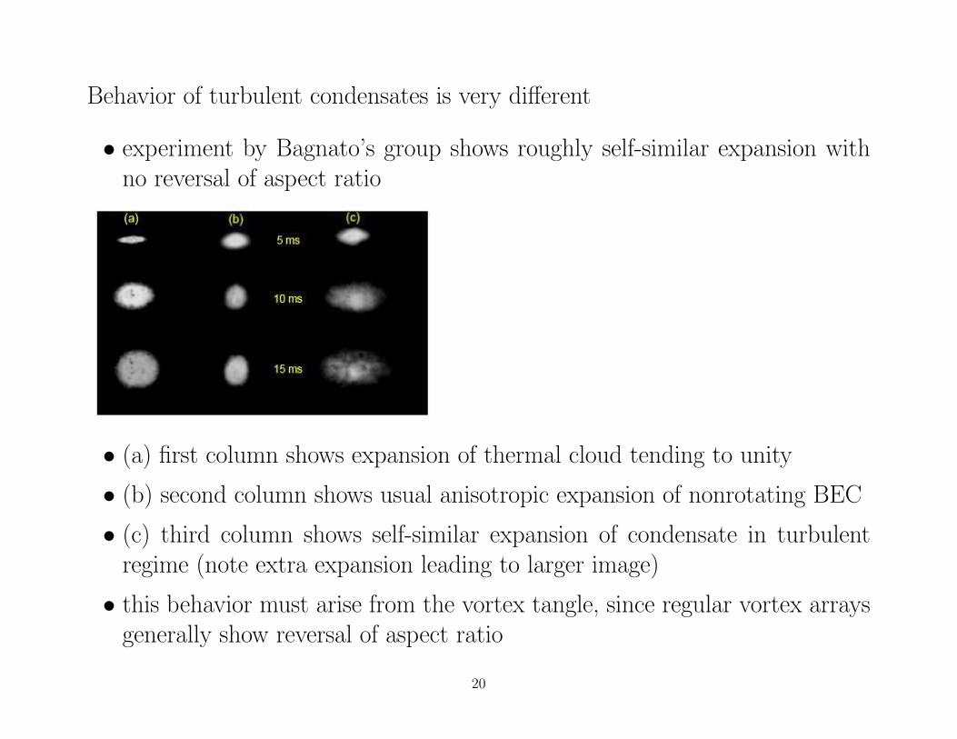
Behavior of turbulent condensates is very different

• experiment by Bagnato’s group shows roughly self-similar expansion withno reversal of aspect ratio

• (a) first column shows expansion of thermal cloud tending to unity

• (b) second column shows usual anisotropic expansion of nonrotating BEC

• (c) third column shows self-similar expansion of condensate in turbulentregime (note extra expansion leading to larger image)

• this behavior must arise from the vortex tangle, since regular vortex arraysgenerally show reversal of aspect ratio

20

4. Theoretical model based on Thomas-Fermi approximation

Recall Euler equation for an ideal (nonviscous) fluid

∂v

∂t+ (v ·∇)v +

1

ρ∇p = f ,

where v is the local velocity, p is the pressure, ρ is the mass density, and f isthe force density (such as gravity)

• this equation is simply Newton’s law applied to a particular element ofmoving fluid (Eulerian picture)

• first two terms are the convective or hydrodynamic derivative

dv

dt=∂v

∂t+ (v ·∇)v

21

• familiar vector identities lead to equivalent form

∂v

∂t+ ∇

(12v

2)

+1

ρ∇p = f + v × (∇× v)

• for an incompressible irrotational fluid with ∇ × v = 0, the velocity maybe expressed by a velocity potential v = ∇Φ

• for an external potential with f = −∇V , this immediately yields Bernoulli’sequation

∇(

12v

2 +p

ρ+ V +

∂Φ

∂t

)= 0

• in presence of vorticity, need to retain term v × (∇× v)

• for solid-body rotation with angular velocity Ω, velocity is v = Ω× r and∇× v = 2Ω, so this term becomes 2v ×Ω

• in this latter situation, cannot use velocity potential and need full form ofdynamical equation

22

How do these considerations apply to turbulent BECs?

Recall Feynman’s suggestion (1955) that the areal vortex density in a rotatingsuperfluid should be nv = 2Ω/κ = MΩ/(π~), where κ = 2π~/M is thequantum of circulation

• this result follows by assuming that the mean vorticity nvκ should be theclassical value for solid-body rotation ∇× v = 2Ω

• experiments on rotating BECs with vortex lattices confirm this Feynmanrelation with considerable accuracy

• MIT experiment with up to ∼ 130 vortices

23

Return to full time-dependent GP equation in hydrodynamic form for n and v

• first is conservation of particles

∂n

∂t+ ∇ · (nv) = 0

• second is usual dynamical equation, now written in terms of hydrodynamic(convective) derivative dv/dt = ∂v/∂t + (v ·∇)v

Mdv

dt+ ∇ (Vtr + gn− µ) = 0,

which is just Newton’s law for the superfluid BEC

• here Vtr is confining trap potential, gn describes the repulsive interactionswith g = 4π~2a/M > 0, a ∼ a few nm is the s-wave scattering length, andµ is chemical potential

• here use Thomas-Fermi picture to ignore “quantum pressure” that involves~2 and derivative of density

• note that these equations are written in the laboratory frame of reference

24

• as for ideal classical fluid, expand convective term(v ·∇)v = ∇(1

2v2)− v × (∇× v)

• for dense vortex array, approximate mean vorticity as 〈∇×v〉 ≈ 2Ω, whereΩ follows from Feynman’s relation nv = MΩ/(π~)

• in this way, obtain the new dynamical equation for the superfluid in presenceof distributed mean vorticity

M∂v

∂t+ ∇

(12Mv2 + Vtr + gn− µ

)+ 2MΩ× v = 0

• this approach was used by Sedrakian and Wasserman (2001) and by Cozziniand Stringari (2003)

• gives good description of quadrupole modes in rapidly rotating condensate,including periodic formation of “stripes” in vortex lattice (JILA, 2002)

25

• apply to axisymmetric condensate rotating about symmetry (z) axis withangular velocity Ω

• in equilibrium, mean velocity in laboratory frame 〈vs〉 ≈ Ω × r leads tofamiliar Thomas-Fermi condensate radii that now depend on Ω

R⊥(Ω)2 =2µ(Ω)

M(ω2⊥ − Ω2)

and Rz(Ω)2 =2µ(Ω)

Mω2z

,

where µ(Ω) = µ(0)(1− Ω2/ω2

⊥)2/5

, with µ(0) for a nonrotating condensate

• aspect ratio Rz(Ω)/R⊥(Ω) =√ω2⊥ − Ω2/ωz now depends on Ω

• provides good diagnostic method to infer angular velocity (JILA)

26

Now apply these ideas to expansion of the condensate when trapis turned off

• goal is to describe free expansion of a BEC containing fluctuating angularmomentum along all different directions (a vortex tangle)

• as first attempt, consider simpler situation with angular momentum alongeach principal axis of axisymmetric condensate

• focus on two limiting cases to develop some intuition about the dynamics

• parametrize the density as follows (this is the usual Thomas-Fermi model)

n(r, t) = n0(t)

(1− x2

Rx(t)2− y2

Ry(t)2− z2

Rz(t)2

)• n0(t) is given by usual Thomas-Fermi normalization condition

n0(t) =15N

8π Rx(t)Ry(t)Rz(t)

27

First assume uniform vortex array along the symmetry axis z

• here Ω is along symmetry axis (z)

• assume velocity has both irrotational part caused by the expansion andsolid-body part from the uniform vortex array

v = 12∇[bx(t)x

2 + by(t)y2 + bz(t)z

2]︸ ︷︷ ︸

irrotational expansion flow

+ Ω× r︸ ︷︷ ︸rotational flow

• substitute these expressions into the dynamical equations assuming thattrap potential vanishes for t > 0

28

• find coupled second-order differential equations for evolution of condensateradii

Rx =15N~2a

M 2

1

R2xRyRz

+

(Nv~M

)21

RxR2y

with similar equation for Ry, where Nv is total number of vortices (thisnumber is conserved), and

Rz =15N~2a

M 2

1

R2zRxRy

• note role of repulsive interaction (a > 0) in expanding in all three directions

• initial Rz is large, so axial expansion (∝ R−2z ) is small, leading to reversal

of aspect ratio for usual condensate

29

• repeat transverse equations

Rx =15N~2a

M 2

1

R2xRyRz

+

(Nv~M

)21

RxR2y

with similar equation for Ry, where Nv is total number of vortices (thisnumber is conserved)

• note directions perpendicular to Ω (namely those along x and y) experienceadditional outward force proportional to N 2

v (and hence proportional toinitial Ω2)

• vortex lines experience effective mutual repulsive interactions (like magneticfield lines in a plasma)

• for large times, interaction terms (∝ a) are smaller than rotation terms(∝ N 2

v ) by one factor of R−1

• numerical studies yield the time-dependent aspect ratio (condensate hereremains axisymmetric)

30

• left side shows typical geometry of condensate with Ω along symmetry axis

• right side shows evolution of aspect ratio R⊥/Rz for various initial vortexdensities

• as anticipated, presence of axial vorticity (along z) enhances the radialexpansion and hence the aspect ratio during expansion

31

Next assume uniform vortex array perpendicular to thesymmetry axis

• specifically, assume Ω = Ωx

• now rotating condensate is not symmetric about rotation axis

• this rotating asymmetry induces an additional irrotational flow induced bythe moving boundary

• induced velocity potential is proportional to Ωyz; corresponding inducedirrotational flow is proportional to ∇(Ωyz)

• hence generalize previous assumption for fluid velocity:

v = 12∇[bx(t)x

2 + by(t)y2 + bz(t)z

2]︸ ︷︷ ︸

irrot. expansion flow

+ Ω× r︸ ︷︷ ︸rotational flow

+ α(t) ∇(Ω yz)︸ ︷︷ ︸induced irrot. flow

with

α(t) =R2y(t)−R2

z(t)

R2y(t) + R2

z(t)

32

• now find different coupled second-order differential equations for evolutionof condensate radii

Rx =15N~2a

M 2

1

R2xRyRz

,

Ry =15N~2a

M 2

1

R2yRzRx

+ 4

(Nv~M

)2Ry

(R2y + R2

z)2,

and

Rz =15N~2a

M 2

1

R2zRxRy

+ 4

(Nv~M

)2Rz

(R2y + R2

z)2

• so far, numerical studies ignore the time dependence of initial conditions

• note presence of extra rotation-induced expansion along y and z, but notalong x

33

• evaluate evolution of aspect ratiosRx/Rz andRx/Ry shown below for Ω = 0(nonrotating) and for Ω = 0.7ω⊥

• note that Ω dramatically reduces growth of first aspect ratio

1. for Ω = 0, recover usual reversal of aspect ratio

2. for large Ω, aspect ratio Rx/Rz saturates near unity

• second figure shows that expanding condensate remains nearly axisymmetric

34

5. Variational Lagrangian approach: anisotropic random vorticity

Use variational functional

L =

∫d3r

[i~2

(Ψ∗∂Ψ

∂t− Ψ

∂Ψ∗

∂t

)− E [Ψ]

],

for a trial function Ψ that depends on various variational parameters.

• here the energy density has the Gross-Pitaevski form

E [Ψ] =~2|∇Ψ|2

2M+ Vtr|Ψ|2 +

1

2g|Ψ|4,

where g = 4π~2a/M , with a the s-wave scattering length, and Vtr(r) is thetrap potential (which is turned off at t = 0).

• generalize Thomas-Fermi Ψ to include expansion velocity and vortexvelocity.

• time-dependent terms and interaction energy lead to simple integrals

35

• subtle point is evaluation of vortex contribution

• ignore slow translational motion of vortex tangle

• each vortex has circulating velocity field v = (~/Mr)φ around the localvortex axis

• a single vortex line has kinetic energy per unit length (π~2n/M) ln(r0/ξ),where n is local number density away from core, r0 is inter-vortex distanceand ξ is core radius

• assume a length L of turbulent vortex lines per unit volume

• integral over condensate volume yields approximate vortex energy

Ev ≈Nπ~2

ML ln

(1

L1/2ξ

),

with L−1/2 as the approximate inter-vortex separation.

36

How does vortex line length per unit volume L depend on condensatedimensions?

• assume a total number Nv of vortices in condensate

• for isotropic turbulence, L should scale like√R2x + R2

y + R2z/(RxRyRz)

(I thank G. Baym for discussions on this point)

• geometry of experiments suggests that turbulence is preferentially in xyplane

• hence introduce anisotropy parameter θ and assume

L ≈ Nv

√sin2 θ

(R2x + R2

y

)+ cos2 θ R2

z

RxRyRz

• θ = π/4 is isotropic case, and θ ≈ π/2 describes turbulence in xy plane

37

Lagrangian approach eventually yields dynamical equations for the expansionradii

2

7MR⊥ = − ∂U

∂R⊥and

1

7MRz = − ∂U

∂Rz

• here, U is an effective potential

U(R⊥, Rz) =15

7

~2Na

MR2⊥Rz︸ ︷︷ ︸

interactions

+π~2Nv

M

√2 sin2 θ R2

⊥ + cos2 θ R2z

R2⊥Rz

ln

(1

L1/2ξ

)︸ ︷︷ ︸

turbulent vortices

with separate terms arising from the repulsive interactions and from theturbulent vortices

• interaction term is of order R−3 and dominates for short time

• vortex term is of order R−2 and dominates for large time

• turbulent vortex term here contains only Nv, in contrast to N 2v for uniform

vortex array (because of random cancellation)

38

Typical experimental values for Brazil trap are:

• number of 87Rb atoms N = 2× 105

• ω⊥ = 2π × 207 Hz and ωz = 2π × 23 Hz

• leads to geometric mean angular frequency ω0 =(ω2⊥ωz)1/3

= 625 s−1

• mean bare trap size is d0 =√

~/Mω0 = 1.08 µm (this ignores repulsion)

• use ω−10 and d0 as units of time and distance

• initial condensate radii in these units are R⊥ = 3.30 and Rz = 29.7(cigar shaped)

• initial vortex core size is small ξ = 0.146

• assume number of vortices Nv ≈ 100

39

Integrate resulting equations of motion for 0 ≤ t ≤ 200 (this is about 0.3 s)

• need to assume anisotropy parameter θ ≈ π/2 (random vorticity in xyplane) since otherwise vorticity in z direction enhances radial expansion

• condensate expands radially initially but saturates with aspect ratioR⊥/Rz ≈2.5 (experiment suggests this ratio is of order one)

• solid line is vortex-free condensate and dashed line is turbulent condensate

• if number of vortices is Nv ≈ 200, then aspect ratio saturates near 2

40

Comments, Discussion, and Conclusions

Here, explain qualitatively the anomalous self-similar expansion of turbulentcondensate

• first use macroscopic toy model based on rotational dynamics with uniformdistributed vorticity aligned perpendicular to symmetry axis of condensate

• based on experimental geometry that couples applied excitationpreferentially to axes perpendicular to symmetry axis

• leads to significant reduction of aspect-ratio inversion

• second use Lagrangan variational method to include random turbulentvorticity (preferentially in xy plane)

• both models lead to roughly self-similar expansion of turbulent condensate,but details are not quantitatively correct

41

Acknowledgments

I thank Vanderlei Bagnato for terrific hospitality during visits to Sao Carlos(Brazil) and Monica Caracanhas for valuable discussions and many numericalstudies of expanding condensates. Many discussions with Gordon Baym inAspen helped understand how to include the random vorticity in the Lagrangianformalism.

42