Self Organizing Fuzzy Neural Networks
6
Forecasting Time Series by SOFNN with Reinforcement Learning Takashi Kuremoto, Masanao Obayashi, and Kunikazu Kobayashi Abstract— A self -org anize d fuzz y neur al network (SOFNN) with a reinforcement learning algorithm called Stochastic Gra- dient Ascent (SGA) is proposed to forecast a set of 11 time series. The proposed system is confirmed to predict chaotic time series before, and is applied to predict each/every time series in NN3 for ecas ting compe titio n modif ying parameter s of thre shold of fuzzy neurons only. The training results are obviously effective and results of long-term prediction give convincible trend values in the future of time series. I. I NTRODUCTION Though many artificial neural networks (ANN) are suitable to forecast time series, radial basis function network (RBFN) is still recommend to be applied on chaotic time series [1], [2], [3] and financial time series [4]. Meanwhile, how to de- sign the structure of hidden-layer in RBFN is a puzzling and confu sing problem in pract ice. Leung and Wang propose d a techn ique called the cross -validated subsp ace metho d to estimate the optimum number of hidden units, and applied the method to pre dic tion of noi sy chaoti c time ser ies [3] but the method may fall its ef fici enc y whe n the traini ng sample dat a is not enough. To ov erc ome the proble m of RBFN, we proposed a self-organization fuzzy network and its ef fec ti ven ess on pre dic tion of cha oti c time ser ies wa s investigated [5], [6]. Furthermore, the learning algorithm is so important to any artificial neural network. Reinforcement learning (RL), a kind of goal-directed learning, is well known for an agent adapting unknown environments [7], [8]. We have proposed to apply a kind of RL cal led stochast ic gra die nt asc ent (SGA) on nonlinear predations [5], [6], [9]. The accurate of forecasting in experiments using Lorenz chaotic time series shown its good efficiency whatever the type of ANN is either multi- layer perception (MLP) or SOFNN. In this pa pe r , we inte nd to use SOFNN an d SGA to forecast a set of 11 time series given by neural forecasting competition (NN3) [10]. The prediction system is introduced in Section 1 in detail, and all of train forecasting results and forecasting results are shown in Section 2. II. FORECASTING SYSTEM Flow of forecasting is shown in Fig. 1 and self-organized fuzzy neural network, ANN predictor, is a RBF-like neural network (Fig. 2). The input layer is given by data in history of time series (Subse cti on 2.1). The hidden lay er consis ts Gaus sian membersh ip funct ions which numbe r is deci ded by a threshold and the rule lay er rea liz es fuz zy inf ere nce (Subsection 2.2 and 2.3). Forecasting is executed according Authors are with the Graduate School of Science and Systems Engineer- ing, Yamaguchi University , Tokiwadai 2-16-1, Ube, Yamaguchi 755-8611, Japan, Tel: +81-836-859520, Fax: +81-836-859501, Email: {wu, m.obayas, koba}@yamaguchi-u.ac.jp to a pr obabil it y poli cy whic h to de te rminate acti ons in the proced ure of rei nforce ment lea rni ng and the err or of forecasting is as reward value (Subsection 2.4). A. Embe dding According to the Takens embedding theorem, the inputs of prediction system on time t, can be reconstructed as a n dimen sion s vect or space X (t), which includes n observed points with same intervals on a time series y(t). X (t) = (x 1 (t),x 2 (t), ··· ,x n (t)) (1) = (y(t), y(t − τ ), ··· ,y(t − (n − 1)τ ) (2) where τ is ti me dela y (in terv al of sa mpli ng) ma y be an arbit rary value in theor y but it effe cts predictio n accur acy in practice, n is the embedding dimension, n > 1. B. Self-organiz ed Fuzzy Neural Network (SOFNN) Fig. 2 shows an architecture of self-organized fuzzy neu- ral network (SOFNN) we proposed. The initial number of membership function and fuzzy rule is only 1, respectively. 1) Memb ers hip Func tion: T o each element x i (t) of the input X (t), membe rship funct ion B ij (x i (t)) is repre sente d as B ij (x i (t)) = exp − (x i (t) − m ij ) 2 2σ 2 ij (3) where m ij and σ ij are the parameters of mean and standard deviation of the Gaussian membership function in j th node, respectiv ely. Initially , j = 1, and with increasing of input patterns, the new membership function will be added. y(t) X(t) Evaluation of Prediction Reinforcement learning y(t+1) ^ Time Series Reconstructed Inputs Self-organized Fuzzy Neural Network Prediction under Stochastice Policy r: reward Fig. 1. Flow chart o f train ing and f orecas ting.
-
Upload
jonathanshore3401 -
Category
Documents
-
view
231 -
download
0
Transcript of Self Organizing Fuzzy Neural Networks
8/8/2019 Self Organizing Fuzzy Neural Networks
http://slidepdf.com/reader/full/self-organizing-fuzzy-neural-networks 1/5
Forecasting Time Series by SOFNN with Reinforcement Learning
Takashi Kuremoto, Masanao Obayashi, and Kunikazu Kobayashi
Abstract— A self-organized fuzzy neural network (SOFNN)with a reinforcement learning algorithm called Stochastic Gra-
dient Ascent (SGA) is proposed to forecast a set of 11 time series.The proposed system is confirmed to predict chaotic time seriesbefore, and is applied to predict each/every time series in NN3forecasting competition modifying parameters of threshold of fuzzy neurons only. The training results are obviously effectiveand results of long-term prediction give convincible trend valuesin the future of time series.
I. INTRODUCTION
Though many artificial neural networks (ANN) are suitable
to forecast time series, radial basis function network (RBFN)
is still recommend to be applied on chaotic time series [1],
[2], [3] and financial time series [4]. Meanwhile, how to de-sign the structure of hidden-layer in RBFN is a puzzling and
confusing problem in practice. Leung and Wang proposed
a technique called the cross-validated subspace method to
estimate the optimum number of hidden units, and applied
the method to prediction of noisy chaotic time series [3]
but the method may fall its efficiency when the training
sample data is not enough. To overcome the problem of
RBFN, we proposed a self-organization fuzzy network and
its effectiveness on prediction of chaotic time series was
investigated [5], [6].
Furthermore, the learning algorithm is so important to any
artificial neural network. Reinforcement learning (RL), a kind
of goal-directed learning, is well known for an agent adaptingunknown environments [7], [8]. We have proposed to apply
a kind of RL called stochastic gradient ascent (SGA) on
nonlinear predations [5], [6], [9]. The accurate of forecasting
in experiments using Lorenz chaotic time series shown its
good efficiency whatever the type of ANN is either multi-
layer perception (MLP) or SOFNN.
In this paper, we intend to use SOFNN and SGA to
forecast a set of 11 time series given by neural forecasting
competition (NN3) [10]. The prediction system is introduced
in Section 1 in detail, and all of train forecasting results and
forecasting results are shown in Section 2.
II . FORECASTING SYSTEM
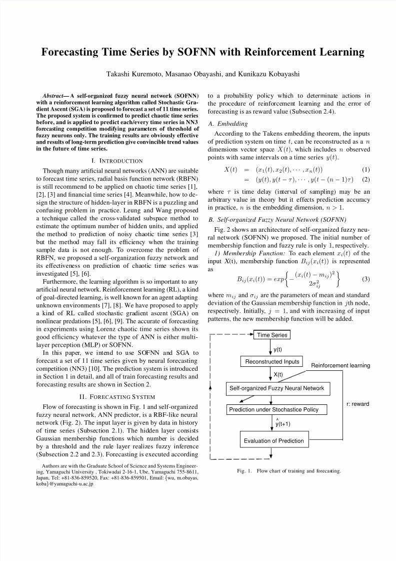
Flow of forecasting is shown in Fig. 1 and self-organized
fuzzy neural network, ANN predictor, is a RBF-like neural
network (Fig. 2). The input layer is given by data in history
of time series (Subsection 2.1). The hidden layer consists
Gaussian membership functions which number is decided
by a threshold and the rule layer realizes fuzzy inference
(Subsection 2.2 and 2.3). Forecasting is executed according
Authors are with the Graduate School of Science and Systems Engineer-ing, Yamaguchi University , Tokiwadai 2-16-1, Ube, Yamaguchi 755-8611,Japan, Tel: +81-836-859520, Fax: +81-836-859501, Email: {wu, m.obayas,koba}@yamaguchi-u.ac.jp
to a probability policy which to determinate actions inthe procedure of reinforcement learning and the error of
forecasting is as reward value (Subsection 2.4).
A. Embedding
According to the Takens embedding theorem, the inputs
of prediction system on time t, can be reconstructed as a n
dimensions vector space X (t), which includes n observed
points with same intervals on a time series y(t).
X (t) = (x1(t), x2(t), · · · , xn(t)) (1)
= (y(t), y(t − τ ), · · · , y(t − (n − 1)τ ) (2)
where τ is time delay (interval of sampling) may be an
arbitrary value in theory but it effects prediction accuracy
in practice, n is the embedding dimension, n > 1.
B. Self-organized Fuzzy Neural Network (SOFNN)
Fig. 2 shows an architecture of self-organized fuzzy neu-
ral network (SOFNN) we proposed. The initial number of
membership function and fuzzy rule is only 1, respectively.
1) Membership Function: To each element xi(t) of the
input X (t), membership function Bij(xi(t)) is represented
as
Bij(xi(t)) = exp
−(xi(t) − mij)2
2σ2ij
(3)
where mij and σij are the parameters of mean and standarddeviation of the Gaussian membership function in jth node,
respectively. Initially, j = 1, and with increasing of input
patterns, the new membership function will be added.
y(t)
X(t)
Evaluation of Prediction
Reinforcement learning
y(t+1)^
Time Series
Reconstructed Inputs
Self-organized Fuzzy Neural Network
Prediction under Stochastice Policyr: reward
Fig. 1. Flow chart of training and forecasting.
8/8/2019 Self Organizing Fuzzy Neural Networks
http://slidepdf.com/reader/full/self-organizing-fuzzy-neural-networks 2/5
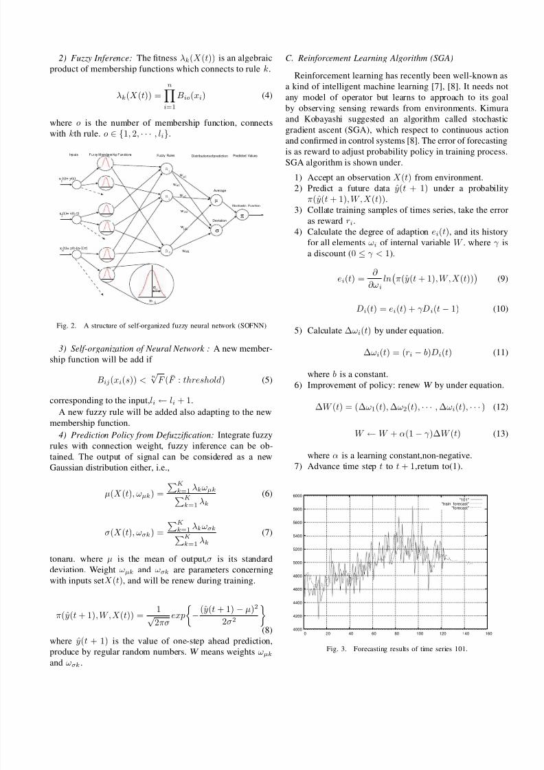
2) Fuzzy Inference: The fitness λk(X (t)) is an algebraic
product of membership functions which connects to rule k.
λk(X (t)) =
ni=1
Bio(xi) (4)
where o is the number of membership function, connects
with kth rule. o ∈ {1, 2, · · · , li}.
R1
R2
R K
R
R
R
R
R
R
σ
σ
mij
ij
µ
wµ1
µ2
µΚ
σ1
σ2
σΚ
w
w
w
w
w
π
x (t)= y(t)
x (t)= y(t-τ)
x (t)= y(t-(n-1)τ)
1
2
n
Inputs Fuzzy Membership Funct ions Fuzzy Rules Distributions of prediction Predicted Values
Average
Deviation
Stochastic Function
Fig. 2. A structure of self-organized fuzzy neural network (SOFNN)
3) Self-organization of Neural Network : A new member-
ship function will be add if
Bij(xi(s)) <n√
F (F : threshold) (5)
corresponding to the input,li ← li + 1.A new fuzzy rule will be added also adapting to the new
membership function.
4) Prediction Policy from Defuzzification: Integrate fuzzy
rules with connection weight, fuzzy inference can be ob-
tained. The output of signal can be considered as a new
Gaussian distribution either, i.e.,
µ(X (t), ωµk) =
Kk=1 λkωµkKk=1 λk
(6)
σ(X (t), ωσk) = Kk=1 λkωσkKk=1 λk
(7)
tonaru. where µ is the mean of output,σ is its standard
deviation. Weight ωµk and ωσk are parameters concerning
with inputs setX (t), and will be renew during training.
π(y(t + 1), W , X (t)) =1√2πσ
exp
− (y(t + 1) − µ)2
2σ2
(8)
where y(t + 1) is the value of one-step ahead prediction,
produce by regular random numbers. W means weights ωµk
and ωσk .
C. Reinforcement Learning Algorithm (SGA)
Reinforcement learning has recently been well-known as
a kind of intelligent machine learning [7], [8]. It needs not
any model of operator but learns to approach to its goal
by observing sensing rewards from environments. Kimura
and Kobayashi suggested an algorithm called stochastic
gradient ascent (SGA), which respect to continuous action
and confirmed in control systems [8]. The error of forecasting
is as reward to adjust probability policy in training process.
SGA algorithm is shown under.
1) Accept an observation X (t) from environment.
2) Predict a future data y(t + 1) under a probability
π(y(t + 1), W , X (t)).
3) Collate training samples of times series, take the error
as reward ri.
4) Calculate the degree of adaption ei(t), and its history
for all elements ωi of internal variable W . where γ is
a discount (0 ≤ γ < 1).
ei(t) =∂
∂ωiln
π(y(t + 1), W , X (t))
(9)
Di(t) = ei(t) + γDi(t − 1) (10)
5) Calculate ∆ωi(t) by under equation.
∆ωi(t) = (ri − b)Di(t) (11)
where b is a constant.
6) Improvement of policy: renew W by under equation.
∆W (t) = (∆ω1(t), ∆ω2(t), · · · , ∆ωi(t), · · · ) (12)
W ← W + α(1 − γ )∆W (t) (13)
where α is a learning constant,non-negative.
7) Advance time step t to t + 1,return to(1).
4000
4200
4400
4600
4800
5000
5200
5400
5600
5800
6000
0 20 40 60 80 100 120 140 160
"101""train_forecast"
"forecast"
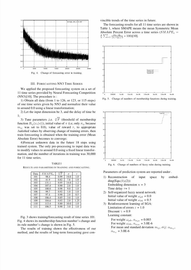
Fig. 3. Forecasting results of time series 101.
8/8/2019 Self Organizing Fuzzy Neural Networks
http://slidepdf.com/reader/full/self-organizing-fuzzy-neural-networks 3/5
0.7
0.8
0.9
1
1.1
1.2
1.3
1.4
1.5
0 5000 10000 15000 20000 25000 30000
"average_abs_error.dat"
Fig. 4. Change of forecasting error in training.
III . FORECASTING NN3 TIM E SERIES
We applied the proposed forecasting system on a set of
11 time series provided by Neural Forecasting Competition
(NN3)[10]. The procedure is :
1) Obtain all data (from 1 to 126, or 123, or 115 steps)
of one time series given by NN3 and normalize their value
to around 0.0 using a linear transformation;
2) Let the input dimension be 3, and the delay of time be
1;
3) Tune parameters ,i.e.n√
F (threshold of membership
function Bij(xi(s))), initial value of π (i.e, only σij because
mij was set to 0.0), value of reward r, to appropriate
/satisfied values by observing change of training errors, then
train forecasting is obtained when the training error (Mean
Absolute Error) becomes to converge;
4)Forecast unknown data in the future 18 steps usingtrained system. The only pre-processing to input data was
to modify values to around 0.0 using a fixed linear transfor-
mation, and the number of iterations in training was 30,000
for 11 time series.
TABLE I
RESULTS AND PARAMETERS IN TRAINING AND FORECASTING .
Data S M A P E sn√
F σ r
101 98.4 0.99 10.0 1.0
102 41.9 0.82 7.8 1.0
103 131.1 0.95 14.0 1.2
104 107.4 0.90 2.0 1.0
105 100.0 0.98 9.0 1.0106 99.7 0.92 1.0 1.0
107 97.4 0.90 2.0 0.5
108 106.4 0.85 3.0 1.0
109 104.6 0.92 2.0 1.25
110 113.4 0.80 10.0 1.0
111 106.5 0.90 3.0 1.0
Fig. 3 shows training/forecasting result of time series 101.
Fig. 4 shows its membership function number’s change and
its rule number’s change is shown in Fig. 5.
The results of training shown the effectiveness of our
method, and the results of long-term forecasting gave con-
vincible trends of the time series in future.
The forecasting results for all 11 time series are shown in
Table 1, where SMAPE means the mean Symmetric Mean
Absolute Percent Error across a time series (SMAPE s =1n
nt=1
|xt−yt|(xt+yt)/2
∗ 100)[10].
0
1
2
3
4
5
6
7
8
0 500000 1e+06 1.5e+06 2e+06 2.5e+06 3e+06 3.5e+06 4e+06
"fuzzy1.txt""fuzzy2.txt""fuzzy3.txt"
Fig. 5. Change of numbers of membership functions during training.
0
2
4
6
8
10
12
14
16
0 500000 1e+06 1.5e+06 2e+06 2.5e+06 3e+06 3.5e+06 4e+06
"rule.txt"
Fig. 6. Change of numbers of fuzzy rules during training.
Parameters of prediction system are reported under .
1) Reconstruction of input space by embed-
ding(Equ.(1),(2)):
Embedding dimension n = 3
Time delay τ = 12) Self-organized fuzzy neural network:
Initial value of weight ωµk = 0.0
Initial value of weight ωσk = 0.5
3) Reinforecement learning of SGA:
Limitation of errors ε = 1.0
Discount γ = 0.9
Learning constant:
For weight ωµk, αωµk = 0.003
For weight ωσk , αωσk = 3.0E-6
For mean and standard deviation mij , σij : αmij,
ασij = 3.0E-6
8/8/2019 Self Organizing Fuzzy Neural Networks
http://slidepdf.com/reader/full/self-organizing-fuzzy-neural-networks 4/5
1000
2000
3000
4000
5000
6000
7000
8000
9000
10000
0 20 40 60 80 100 120 140 160
"102""train_forecast"
"forecast"
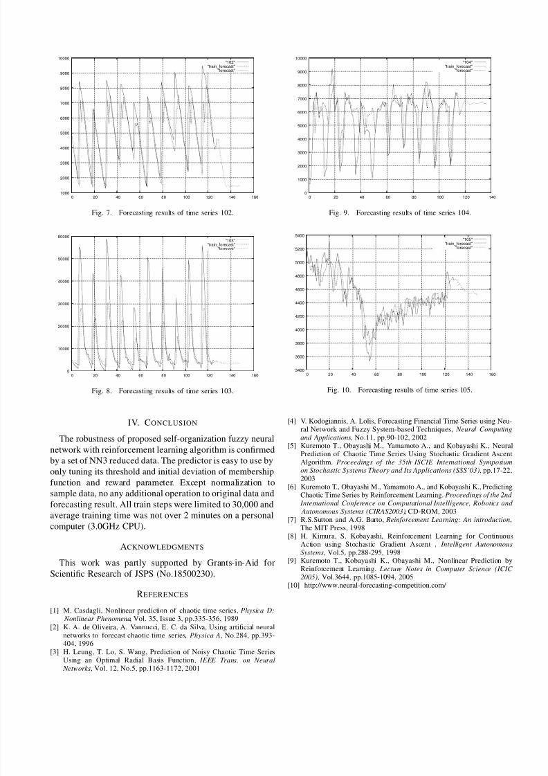
Fig. 7. Forecasting results of time series 102.
0
10000
20000
30000
40000
50000
60000
0 20 40 60 80 100 120 140 160
"103""train_forecast"
"forecast"
Fig. 8. Forecasting results of time series 103.
IV. CONCLUSION
The robustness of proposed self-organization fuzzy neural
network with reinforcement learning algorithm is confirmed
by a set of NN3 reduced data. The predictor is easy to use by
only tuning its threshold and initial deviation of membership
function and reward parameter. Except normalization to
sample data, no any additional operation to original data and
forecasting result. All train steps were limited to 30,000 and
average training time was not over 2 minutes on a personal
computer (3.0GHz CPU).
ACKNOWLEDGMENTS
This work was partly supported by Grants-in-Aid for
Scientific Research of JSPS (No.18500230).
REFERENCES
[1] M. Casdagli, Nonlinear prediction of chaotic time series, Physica D:
Nonlinear Phenomena, Vol. 35, Issue 3, pp.335-356, 1989
[2] K. A. de Oliveira, A. Vannucci, E. C. da Silva, Using artificial neuralnetworks to forecast chaotic time series, Physica A, No.284, pp.393-404, 1996
[3] H. Leung, T. Lo, S. Wang, Prediction of Noisy Chaotic Time SeriesUsing an Optimal Radial Basis Function, IEEE Trans. on Neural
Networks, Vol. 12, No.5, pp.1163-1172, 2001
0
1000
2000
3000
4000
5000
6000
7000
8000
9000
10000
0 20 40 60 80 100 120 140
"104""train_forecast"
"forecast"
Fig. 9. Forecasting results of time series 104.
3400
3600
3800
4000
4200
4400
4600
4800
5000
5200
5400
0 20 40 60 80 100 120 140 160
"105""train_forecast"
"forecast"
Fig. 10. Forecasting results of time series 105.
[4] V. Kodogiannis, A. Lolis, Forecasting Financial Time Series using Neu-ral Network and Fuzzy System-based Techniques, Neural Computing
and Applications, No.11, pp.90-102, 2002[5] Kuremoto T., Obayashi M., Yamamoto A., and Kobayashi K., Neural
Prediction of Chaotic Time Series Using Stochastic Gradient AscentAlgorithm. Proceedings of the 35th ISCIE International Symposium
on Stochastic Systems Theory and Its Applications (SSS’03), pp.17-22,2003
[6] Kuremoto T., Obayashi M., Yamamoto A., and Kobayashi K., PredictingChaotic Time Series by Reinforcement Learning. Proceedings of the 2nd
International Conference on Computational Intelligence, Robotics and
Autonomous Systems (CIRAS2003), CD-ROM, 2003[7] R.S.Sutton and A.G. Barto, Reinforcement Learning: An introduction,
The MIT Press, 1998[8] H. Kimura, S. Kobayashi, Reinforcement Learning for Continuous
Action using Stochastic Gradient Ascent , Intelligent AutonomousSystems, Vol.5, pp.288-295, 1998
[9] Kuremoto T., Kobayashi K., Obayashi M., Nonlinear Prediction byReinforcement Learning. Lecture Notes in Computer Science (ICIC
2005), Vol.3644, pp.1085-1094, 2005[10] http://www.neural-forecasting-competition.com/
8/8/2019 Self Organizing Fuzzy Neural Networks
http://slidepdf.com/reader/full/self-organizing-fuzzy-neural-networks 5/5
3500
4000
4500
5000
5500
6000
6500
0 20 40 60 80 100 120 140 160
"106""train_forecast"
"forecast"
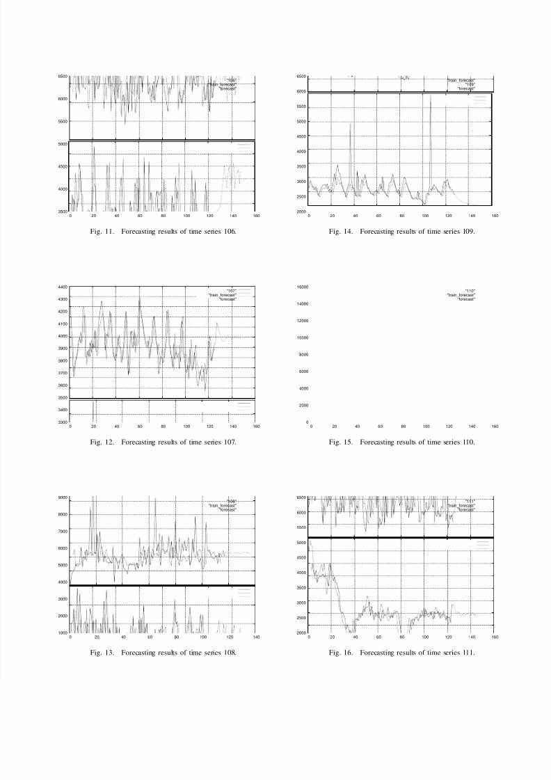
Fig. 11. Forecasting results of time series 106.
3300
3400
3500
3600
3700
3800
3900
4000
4100
4200
4300
4400
0 20 40 60 80 100 120 140 160
"107""train_forecast"
"forecast"
Fig. 12. Forecasting results of time series 107.
1000
2000
3000
4000
5000
6000
7000
8000
9000
0 20 40 60 80 100 120 140
"108""train_forecast"
"forecast"
Fig. 13. Forecasting results of time series 108.
2000
2500
3000
3500
4000
4500
5000
5500
6000
6500
0 20 40 60 80 100 120 140 160
"train_forecast""109"
"forecast"
Fig. 14. Forecasting results of time series 109.
0
2000
4000
6000
8000
10000
12000
14000
16000
0 20 40 60 80 100 120 140 160
"110""train_forecast"
"forecast"
Fig. 15. Forecasting results of time series 110.
2000
2500
3000
3500
4000
4500
5000
5500
6000
6500
0 20 40 60 80 100 120 140 160
"111""train_forecast"
"forecast"
Fig. 16. Forecasting results of time series 111.