Self-Learning 3D Object Classification

Jens Garstka and Gabriele PetersHuman-Computer Interaction, Faculty of Mathematics and Computer Science,

FernUniversitt in Hagen - University of Hagen, D-58084 Hagen, Germanygabriele.peters@fernuni-hagen.de

Keywords: Active Vision, Active Learning, Object Classification, 3D Feature Descriptors, Reinforcement Learning.

Abstract: We present a self-learning approach to object classification from 3D point clouds. Existing 3D feature descrip-tors have been utilized successfully for 3D point cloud classification. But there is not a single best descriptorfor any situation. We extend a well-tried 3D object classification pipeline based on local 3D feature descrip-tors by a reinforcement learning approach that learns strategies to select point cloud descriptors dependingon qualities of the point cloud to be classified. The reinforcement learning framework learns autonomouslya strategy to select feature descriptors from a provided set of descriptors and to apply them successively foran optimal classification result. Extensive experiments on more than 200.000 3D point clouds yielded higherclassification rates with partly more reliable results than a single descriptor setting. Furthermore, our approachproved to be able to preserve classification strategies that have been learned so far while integrating additionaldescriptors in an ongoing classification process.

1 INTRODUCTION

An important step towards an effective scene under-standing is a reliable object classification. A centralrequirement for classification algorithms is their in-variance to varying conditions such as location, scale,pose, partial occlusion, or lighting conditions. Thebasic approaches to extract useful information fromimages for either object recognition or classificationare similar and there are a lot of surveys available(Sunet al., 2006; Li and Allinson, 2008; Andreopoulos andTsotsos, 2013; Loncomilla et al., 2016).

While initially the application scenarios had astrong focus on facial recognition, the spectrum be-came significantly more diverse with the introduc-tion of reliable local 2D feature descriptors. Finally,due to the results of deep convolutional neural net-works (Ciresan et al., 2012), the research in this areareceived new impetus that continues to the presentday. However, there are some cases in which the pre-viously mentioned image-based approaches to objectclassification do not work properly on principle. Thisapplies to situations where no structured image infor-mation is available, e.g., when the lighting is insuffi-cient or the objects are monochrome and due to theirshape without sufficient shading. Figure 1 shows twoexamples that reflect such situations, where additional

3D information in form of 3D point clouds could helpto improve object classification.

Figure 1: Examples of objects where a classification solelyon the basis of color information could be difficult.(left image: Francis Tiangson, Pinterest).

In this work we present an approach to object clas-sification based on local feature descriptors for 3Dpoint clouds. Particularly, the focus is not on a sin-gle local 3D feature descriptor, since the 3D objectclassification results of any single descriptor vary a lotdepending on the density and structure of a 3D pointcloud. Instead, the approach presented is essentiallybased on a machine learning method. We use a re-inforcement learning framework to adaptively selectand apply different 3D feature descriptors dependingon the 3D point cloud to be classified. This leads toa clear improvement of the classification results com-pared to the use of single local 3D feature descriptorsonly. The paper is divided into the following sections:

Garstka, J. and Peters, G.Self-Learning 3D Object Classification.In Proceedings of the 7th International Conference on Pattern Recognition Applications and Methods (ICPRAM 2018), pages 511-519ISBN: 978-989-758-276-9Copyright © 2018 by SCITEPRESS – Science and Technology Publications, Lda. All rights reserved

511

Section 2 provides an overview of the methods rele-vant in the context of this work. Section 3 introducesour proposed approach and describes its componentsin detail. Section 4 describes the experiments and in-termediate results. The final 3D object classificationresults are summarized in Section 5. Finally, Sec-tion 6 provides an outlook to future extensions andadaptations of the presented approach. The approachproposed in this work including all parameters of themodel and extended experiments are described in de-tail in (Garstka, 2016).

2 RELATED WORK

This section starts with a brief overview of relatedkeypoint detectors (subsection 2.1) and local 3D fea-ture descriptors for 3D point clouds (subsection 2.2).The majority of currently available algorithms forkeypoint detection and local 3D feature descriptorsare summarized in a survey of 3D object recogni-tion methods by (Guo et al., 2014). Thus, only algo-rithms and approaches that are relevant for our workare quoted below. This is followed by a subsectionon classification approaches for 3D point clouds (sub-section 2.3) and a short introduction of Q-Learning asa reinforcement learning technique we utilize for ourapproach (subsection 2.4).

2.1 Keypoint Detectors

Computational costs of local 3D feature descriptorsare mostly high. It does not make sense to computefeature vectors for all points of a point cloud. We use akeypoint detector to reduce the number of feature vec-tors. Based on the evaluations of (Salti et al., 2011)and (Filipe and Alexandre, 2014) we use the keypointdetector introduced in context of the shape signaturefeature descriptor (ISS) by (Zhong, 2009).

2.2 Local 3D Feature Descriptors

In this subsection, we give an overview of those lo-cal 3D feature descriptors used in the context of thiswork. In short, we use five local 3D feature descrip-tors for 3D point clouds: The spin image (SI) intro-duced by (Johnson and Hebert, 1998) is a 2D his-togram that is rotated around the normal vector ofa point. The point feature histogram (PFH) and thefast point feature histogram (FPFH) collect informa-tion from a local environment based on the so-calledDarbeaux frame. Both were introduced by (Rusuet al., 2008). The signature of histograms of orien-tations (SHOT) by (Tombari et al., 2010b) is a set

of histograms of angles determined for multiple seg-ments of a spherical environment. The values of thesehistograms are concatenated to a signature. And fi-nally the unique shape context (USC) by (Tombariet al., 2010a), which is a normal aligned sphericalhistogram. These local 3D feature descriptors havebeen selected because of their broad spectrum of dif-ferent properties. Two approaches, SI and USC usehistograms, PFH and FPFH create signatures usingsurface properties and SHOT is a hybrid solution ofhistograms and surface properties. The dimensions ofthe feature descriptions should cover the largest pos-sible range, from FPFH with 33 dimensions to USCwith 1960 dimensions. In the same way the speed ofthe descriptors should cover a large range, from SI,which is the fastest to PFH which is more than 1000times slower. Finally, three of the descriptors requirea local reference frame (SHOT, SI, and USC) and theothers do not (FPFH and PFH).

2.3 3D Classification Approaches

A common way to classify an object based on agiven set of local feature descriptions consists of twosteps. The first step is inspired by text categoriza-tion approaches, e.g., (Joachims, 1998). This so-called bag-of-words representation has become an el-igible method for categorizing visual content. Anearly approach is the visual categorization with bagsof keypoints (Csurka et al., 2004). The basic ap-proach consists of mapping high-dimensional vectors,whose values are usually continuous, to a finite setof quantized representatives. These representativesform the so-called visual vocabulary. A histogramin the same size as the vocabulary is used to count themapped feature descriptions and is called frequencyhistogram. Therefore, the method is often referred toas a bag-of-features in this context. In a second stepthese frequency histograms are used as input vectorsfor classifiers. Support vector machines (SVM) areoften used as a classifier. Primarily, SVMs are binaryclassifiers. Therefore, each object class requires itsown SVM. The frequency histogram is then appliedseparately to the SVM of each object class. There arenumerous approaches that follow this basic principle,e.g., (Madry et al., 2012; Yang et al., 2014).

2.4 Reinforcement Learning –Q-Learning

A reinforcement learning (RL) system consists of anagent that interacts with an environment. Based on thecurrent state st of the environment at time t the agentdecides with respect to the learned experience what

ICPRAM 2018 - 7th International Conference on Pattern Recognition Applications and Methods

512

action at will be performed next. The experiencearises from consequences the agent undergoes withinthe environment, i.e., a positive or negative rewardrt+1, which reflects whether the action at was appro-priate to bring the agent closer to its goal (Sutton andBarto, 1998). Q-learning (Watkins and Dayan, 1992)is an algorithm to solve the reinforcement problemfor a finite number of discrete states of a fully ob-servable environment. It determines values which de-scribe the quality of an action a ∈ A(s) for a states ∈ S . These so-called Q-values can be used for amapping π called policy between the current state andthe next action. Q-learning updates its Q-values usingaction at in state st at time t while observing Q-valuesof the next state st+1 and the immediate reward rt+1:

Q(st ,at) = Q(st ,at)+

α[rt+1 + γmax

aQ(st+1,a)−Q(st ,at)

], (1)

where α is a parameter that controls the learning rateand γ is the discount rate with 0 ≤ γ ≤ 1. The lat-ter determines how strongly immediate rewards areweighted compared to future rewards. In this way thereturn, i.e., the total discount of future rewards, forstate-action pairs is estimated. Initially, all Q-valuesare initialized with a constant value, typically zero.In this phase, the Q-values cannot be used for deci-sions. Therefore, the actions are typically selectedrandomly with a probability ε = 1.0. Or in otherwords: the RL agent follows a random policy. Thisphase is called exploration phase. As soon as theQ values get more stable, the portion of randomlyselected actions ε is successively reduced. This isthe transition to the exploitation phase where the RLagent follows a so-called ε-greedy policy. As long asε 6= 0, Q-learning can react to changes in the behav-ior of the environment and makes adjustments to theQ-values. Q-learning is proven to converge to an op-timal value, which means that the best possible wayto solve a given task can be dictated by taking actionsgreedily with respect to the learned Q-values (greedy-policy) (Watkins and Dayan, 1992).

3 METHODS

In our approach several local 3D feature descriptorsare autonomously selected and applied to a 3D pointcloud to be classified. This is not achieved by a one-time optimization of the classification pipeline but bya continuous learning process, which has been imple-mented in the form of a RL framework (Sutton andBarto, 1998). The basic structure of the classifica-tion pipeline is presented in Subsection 3.1 and is ex-

tended with the RL framework as described in Sub-section 3.3. Subsection 3.4 shows how the adaptive-ness of Q-learning is adopted to add local 3D pointcloud descriptors dynamically during ongoing classi-fication processes.

3.1 Classification Pipeline

The structure of the basic classification pipeline isschematically shown in Figure 2. Within this pipelinesome parameters have to be defined in advance. Wetake these parameters from an evaluation describedin (Garstka and Peters, 2016). The dataset used in the

Keypoint

DetectionPoint Cloud

Feature

Description

Bag of

Features

Vocabulary SVMs

Classiଏca-

tion

v o e t

Figure 2: The structure of the basic classification pipeline,which is extended later by a RL approach.

context of this work is the RGB-D Object Dataset ofthe University of Washington (Lai et al., 2011). Thedataset contains 51 object classes with 300 differentobjects where each object was captured in differentposes, resulting in 207841 distinct point clouds, orapproximately 4000 point clouds per object class onaverage. We use only the 3D point cloud data of thedataset for our experiments. Apart from the completeset of 3D point clouds, we also use a reduced set of3D point clouds, which only consists of 10 of the 51object classes (see Figure 3).

Figure 3: One view of one object for each of the 10 se-lected object classes. These are left to right, top to bottom:cap, coffee mug, food bag, greens, hand towel, keyboard,kleenex, notebook, pitcher, and shampoo.

The classification pipeline starts with a keypointdetection algorithm. As already noted in Section 2.1,we use the ISS keypoint algorithm introduced byZhong. The average number of keypoints determinedby ISS on the given set of point clouds is approx. 131.In the second step the basic classification pipelinecontinues with the computation of a local 3D featuredescription at each keypoint. The descriptors usedhave been presented in Section 2.2. Next, the cal-culated feature descriptions are sorted into the bag offeatures frequency histogram. Beforehand, the num-ber of visual words of the vocabulary, i.e., the num-

Self-Learning 3D Object Classification

513

KeypointDetectionPoint Cloud Feature

DescriptionBag of

Features

Vocabulary SVMs

Classifica-tion

Environment

AgentState

Actions3D FeatureDescriptors

Class-CandidatesPolicy

Q-Table Update Q-Table

reward -1,[0,3[new

state

action

Class-Candidates

Cloud-PropertiesComputeProperties

Figure 4: Extension of the classification pipeline with a RL framework.

ber of bins of the frequency histogram, has to be de-fined. Within the scope of preceding evaluations weobtained best results with vocabulary sizes of 50 forSI, 100 for PFH, FPFH and SHOT, and 200 for USC,which are also used for the experiments described inSection 4. The vocabulary is determined using k-means++ (Arthur and Vassilvitskii, 2007) with an Eu-clidean distance.

The last step of the pipeline is the classification.Each object class is bound to a set of correspondingSVMs, one for each local 3D feature descriptor. Thekernel function used in SVMs is a Gaussian radial ba-sis function. The best parameter values are taken froman evaluation described in (Garstka and Peters, 2016)quoted above: the kernel parameter γ = 0.008 and theSVM penalty parameter C = 125. All SVMs havebeen trained using every second point cloud of thecorresponding object class as positive example, whichare ≈ 2000 3D point clouds. The double amount of≈ 4000 randomly selected 3D point clouds from allother object classes have been used as negative exam-ples.

3.2 Reference Values

In order to obtain an average classification rate foreach local 3D feature descriptor, the basic classifi-cation pipeline has been applied for each local 3Dfeature descriptor separately to all 3D point clouds,which were not used for the training of the SVMs.In the following this setting is referred to as singledescriptor setting. The results can be divided into 3cases:

1. Exactly for one object class the prediction valueof its SVM is positive, and it is the correct objectclass. This case is hereinafter referred to as anexact match.

2. For several object classes the prediction values oftheir SVMs are positive, but the object class theSVM of which has the highest prediction value

corresponds to the correct object class. The latterwill be hereinafter referred to as the best match.

3. In all other situations the classification fails.

The assignment rates from the first and second caseare summarized as classification rate. Table 1 showsthe classification rates of all individual local 3D fea-ture descriptors while performing the described ba-sic classification pipeline. These values serve as ref-erence values for the subsequent extension of thepipeline with the RL framework. The parameters re-quired for each local 3D feature descriptor were takenfrom the respective original publication for each de-scriptor and from the evaluation described in (Garstkaand Peters, 2016). In the single descriptor setting the

Table 1: Classification rates in the single descriptor setting.The results shown have been obtained for each local 3D fea-ture descriptor applied separately, on the one hand applyingthe basic pipeline on all 51 object classes, on the other handonly on the reduced set of 10 object classes.

classification rate for51 classes 10 classes

desc

ript

or

SI 7.4% 23.8%PFH 6.0% 62.9%FPFH 9.4% 65.0%SHOT 3.6% 22.8%USC 8.5% 59.7%

portion of the exact class assignments (case 1 of thepreviously described three cases) among the classifi-cation rates is 0% in all cases.

3.3 Reinforcement LearningFramework

The extension of the basic classification pipeline witha RL approach is illustrated in Figure 4 and describedin Subsubsection 3.3.1 to 3.3.3. To extend the basicclassification pipeline with a RL approach the gen-eral proceeding is as follows: Beginning with a 3D

ICPRAM 2018 - 7th International Conference on Pattern Recognition Applications and Methods

514

point cloud, the first step of the basic pipeline, i.e., therecognition of the keypoints, is performed. Next, thefeature descriptions are determined at each keypoint.Instead of using a single descriptor, the RL agent se-lects one of the available descriptors to determine thefeature descriptions. Then the remaining two stepsof the pipeline are executed for the selected descrip-tor. Once the prediction value of the SVM of the re-spective descriptor corresponding to each object classhas been determined, all object classes with a neg-ative prediction value are excluded. The remainingclasses are hereinafter referred to as class candidates.The further procedure depends primarily on the set ofclass candidates. If it contains more than one objectclass, the classification pipeline resumes at the secondstep. In this case, the RL agent selects another unuseddescriptor with which new feature descriptions are de-termined at the already detected keypoints. Then theremaining steps of the pipeline are executed again.The new prediction values corresponding to the re-maining classes are used to further reduce the classcandidates. After a few iterations this process ideallyends up with the one matching object class remain-ing. However, due to the similarity of many objectclasses, this will rarely be the case. To prevent the se-lection of all feature descriptors during each classifi-cation, a restriction of computation time is introduced.As soon as the time limit is exceeded the object classwith the highest prediction value within the remain-ing class candidates is returned as best matching ob-ject class. The implementation of these concepts, thecomponents, and parameters are described in detail inthe following.

3.3.1 Basic Components of the Framework

The environment of the RL framework is defined bythe set of class candidates, which at the beginningcontains all object classes and additional properties ofthe input point cloud (see Figure 4). The point cloudproperties and their associated discrete values are:1. The number of keypoints relative to all objects:

1st quartile: → slight structure → 12nd, 3rd quartile: →medium structure → 24th quartile: → considerable structure → 3

2. The ratio between the two successive eigenvaluesof the covariance matrix of the point cloud, r1 =e2/e1 and r2 = e3/e2, where e1 ≤ e2 ≤ e3:r1 ≤ 3.0∧ r2 ≤ 3.0 → uniform, not flat → 1r1 ≤ 3.0∧ r2 > 3.0 → elongated, not flat → 2r1 > 3.0∧ r2 ≤ 3.0 → uniform and flat → 3r1 > 3.0∧ r2 > 3.0 → elongated and flat → 4

The RL agent knows the current state of the environ-ment, i.e., the class candidates and the point cloud

properties. Based on the state the agent can performan action, i.e., the selection of a local 3D feature de-scriptor the agent has not yet applied. The agent needsa policy to decide which descriptor should be selectednext in the current state. When using Q-learning, poli-cies are usually based on the so-called Q-table, whichcontains a value for each pair of state and action thatreflects how suitable an action is in a given state. Un-der the assumption that the Q-table contains only op-timal Q-values, the agent selects the best local 3Dfeature descriptor for the current state based on thevalues of the Q-table. The selected descriptor leadsto a change of the environment, i.e., a reduced set ofclass candidates. As the Q-table is initially empty, itis build up successively during the classification.

3.3.2 Terminal States and Rewards

The learning mechanism of RL is based on rewards.In general, a reward can be given for each action ain a state s. However, in the context of our classifi-cation framework a decision on the success of a clas-sification is possible only after the classification pro-cess is terminated. Therefore, all possible terminalstates have to be defined first (see Table 2). An ’exact

Table 2: Summary of rewards for terminal states in our RLframework. C is the set of class candidates, nC the numberof all object classes, t the computation time required to geta result, and tmax the time limit.

name reward

term

inal

stat

e 1) exact match 3.0− t/tmax2a) no actions/match 2.0−|C |/nC2b) no actions/miss 1.0−|C |/nC3a) timeout/match 2.0−|C |/nC3b) timeout/miss 1.0−|C |/nC4) fail state −1.0

match’ means that the set of remaining class candi-dates contains only the correct object class while notimeout occurred. In case of the two terminal statesdistinguished for ’no actions’ no local 3D feature de-scriptor is left to select, while in case of the two ter-minal states distinguished for ’timeout’ the compu-tation time limit is exceeded. In both cases ’match’means that the best matching class is the correct ob-ject class while ’miss’ means that the best matchingclass is an incorrect object class. The fourth case ’failstate’ comprises all cases that are not covered by thepreviously stated cases, such as the case that the set ofremaining class candidates does not contain the cor-rect object class while there are still descriptors leftto be selected and no timeout occurred. For 2a) and3a) the best matching object class is determined fromthe set of class candidates by the highest sum of the

Self-Learning 3D Object Classification

515

prediction values over all iterations. In our approachonly terminal states allow a statement of success orfailure. Thus, all other rewards r are initially set toa value of 0. The rewards for the six cases describedabove are shown in Table 2.

3.3.3 Time Constraint

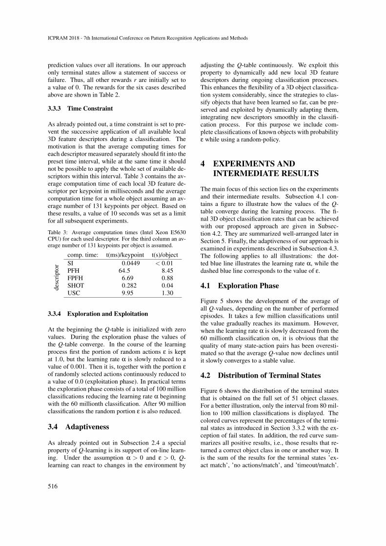
As already pointed out, a time constraint is set to pre-vent the successive application of all available local3D feature descriptors during a classification. Themotivation is that the average computing times foreach descriptor measured separately should fit into thepreset time interval, while at the same time it shouldnot be possible to apply the whole set of available de-scriptors within this interval. Table 3 contains the av-erage computation time of each local 3D feature de-scriptor per keypoint in milliseconds and the averagecomputation time for a whole object assuming an av-erage number of 131 keypoints per object. Based onthese results, a value of 10 seconds was set as a limitfor all subsequent experiments.

Table 3: Average computation times (Intel Xeon E5630CPU) for each used descriptor. For the third column an av-erage number of 131 keypoints per object is assumed.

comp. time: t(ms)/keypoint t(s)/object

desc

ript

or

SI 0.0449 < 0.01PFH 64.5 8.45FPFH 6.69 0.88SHOT 0.282 0.04USC 9.95 1.30

3.3.4 Exploration and Exploitation

At the beginning the Q-table is initialized with zerovalues. During the exploration phase the values ofthe Q-table converge. In the course of the learningprocess first the portion of random actions ε is keptat 1.0, but the learning rate α is slowly reduced to avalue of 0.001. Then it is, together with the portion εof randomly selected actions continuously reduced toa value of 0.0 (exploitation phase). In practical termsthe exploration phase consists of a total of 100 millionclassifications reducing the learning rate α beginningwith the 60 millionth classification. After 90 millionclassifications the random portion ε is also reduced.

3.4 Adaptiveness

As already pointed out in Subsection 2.4 a specialproperty of Q-learning is its support of on-line learn-ing. Under the assumption α > 0 and ε > 0, Q-learning can react to changes in the environment by

adjusting the Q-table continuously. We exploit thisproperty to dynamically add new local 3D featuredescriptors during ongoing classification processes.This enhances the flexibility of a 3D object classifica-tion system considerably, since the strategies to clas-sify objects that have been learned so far, can be pre-served and exploited by dynamically adapting them,integrating new descriptors smoothly in the classifi-cation process. For this purpose we include com-plete classifications of known objects with probabilityε while using a random-policy.

4 EXPERIMENTS ANDINTERMEDIATE RESULTS

The main focus of this section lies on the experimentsand their intermediate results. Subsection 4.1 con-tains a figure to illustrate how the values of the Q-table converge during the learning process. The fi-nal 3D object classification rates that can be achievedwith our proposed approach are given in Subsec-tion 4.2. They are summarized well-arranged later inSection 5. Finally, the adaptiveness of our approach isexamined in experiments described in Subsection 4.3.The following applies to all illustrations: the dot-ted blue line illustrates the learning rate α, while thedashed blue line corresponds to the value of ε.

4.1 Exploration Phase

Figure 5 shows the development of the average ofall Q-values, depending on the number of performedepisodes. It takes a few million classifications untilthe value gradually reaches its maximum. However,when the learning rate α is slowly decreased from the60 millionth classification on, it is obvious that thequality of many state-action pairs has been overesti-mated so that the average Q-value now declines untilit slowly converges to a stable value.

4.2 Distribution of Terminal States

Figure 6 shows the distribution of the terminal statesthat is obtained on the full set of 51 object classes.For a better illustration, only the interval from 80 mil-lion to 100 million classifications is displayed. Thecolored curves represent the percentages of the termi-nal states as introduced in Section 3.3.2 with the ex-ception of fail states. In addition, the red curve sum-marizes all positive results, i.e., those results that re-turned a correct object class in one or another way. Itis the sum of the results for the terminal states ’ex-act match’, ’no actions/match’, and ’timeout/match’.

ICPRAM 2018 - 7th International Conference on Pattern Recognition Applications and Methods

516

0 20 40 60 80 100

610×

avg.

Q-v

alue

0.0005

0.001

0.0015

0.002

0.0025

0.003

0.0035

0.004

0.0045

average Q-values

episodes0 20 40 60 80 100

610×

alpha/

epsi

lon

0.1

0.2

0.3

0.4

0.5

0.6

0.7

0.8

0.9

1 average Q-valuesalphaepsilon

Figure 5: This graph shows the development of the averageQ-value during the exploration phase of the RL frameworkdepending on the number of episodes carried out.

The value of the red curve after the final episode thusrepresents the final classification results of our RLapproach in the setting of 51 object classes. The fi-

80 85 90 95 100

610×

% o

f te

rmin

al s

tate

s

distribution of terminal states

episodes80 85 90 95 100

610×

alpha/

epsi

lon

timeout/matchtimeout/miss

exact matchno actions/matchno actions/miss

sum positive

0.3

0.2

0.1

0

30

20

10

Figure 6: This figure shows the distribution of the terminalstates obtained on the full set of 51 object classes depend-ing on the number of performed episodes. The red curverepresents correct 3D object classifications. By reducing αand ε to a value of zero, the final results of the last episodeare based on a greedy policy and represent the best, learnedstrategy to select the descriptors for 3D object classification.

nal distribution of the terminal states after the lastepisode, represented by the endpoints of the curvesshown in Figure 6, is summarized in Table 4, sup-plemented by the percentage of fail states. This tablealso contains the results for the reduced set of 10 ob-ject classes.

4.3 Adaptive Learning

To explore the adaptiveness of the RL framework, weperform similar experiments as described in the sub-sections before. The difference, however, is that thelearning process is started with a reduced set of onlyfour of five local 3D feature descriptors. Accordingly,the values of α and ε are initially 1.0. After 25 mil-lion episodes the learning rate α is reduced to a valueof 0.1. In this way, a potential over-fitting is com-pensated. After 45 million episodes ε is also reduced

Table 4: Distribution of terminal states after the last episodewith ’sum of positive results’ summarizing the percentagesfor the states ’exact match’, ’no actions/match’, and ’time-out/match’ and thus representing the final 3D object classi-fication rate of our approach.

percentage percentage51 classes 10 classes

term

inal

stat

e exact match 0.0% 16.0%no actions/match 5.4% 0.4%no actions/miss 11.0% 0.2%timeout/match 16.1% 58.6%timeout/miss 11.6% 8.5%fail state 55.9% 16.3%sum of positive results 21.5% 75.0%

to a value of 0.1. From this moment on the rein-forcement learning agent is in an exploitation phasewhere classification rates are reasonably high, even if10% of the actions are performed as random descrip-tor selections. Figure 7 illustrates the adaptivenessof our approach for the case that the FPFH descrip-tor (Rusu et al., 2009) is omitted at the beginning,using the reduced set of 10 object classes. WithoutFPFH the classification rate is ≈ 57% (episode 45-50million). After 50 million episodes, FPFH is added

0 20 40 60 80 100

610×%

of te

rmin

al s

tate

s

10

20

30

40

50

60

70

80adaptiveness, descriptor FPFH

episodes0 20 40 60 80 100

610×

alpha/

epsi

lon

0

0.1

0.2

0.3

0.4

0.5

0.6

0.7

0.8

0.9

1

timeout/matchtimeout/miss

exact matchno actions/matchno actions/miss

sum positive

Figure 7: This graph illustrates the adaptiveness of our ap-proach adding FPFH to the set of descriptors (at 50 mil-lion episodes). The curves represent the distribution ofthe terminal states depending on the number of performedepisodes.

to the list of available descriptors. This is indicatedby the red dashed line in Figure 7. Immediately after-wards the number of correct classifications increasessignificantly within a few episodes and stabilizes tothe value of about ≈ 67%. The difference of ≈ 67%to the result of 75% that was reported in Section 4.2 isdue to the increased portion of random descriptor se-lections and the adapted learning rate. If both, α andε, were set to zero the results would be identical.

Self-Learning 3D Object Classification

517

Figure 8: These images show examples from the reduced set of 10 object classes. The upper row shows images from anobject in a specific pose where classification yielded the best result, while the lower row shows an object from the same objectclass where classification yielded the worst result. The overall geometry for most of the classes is similar for best and worstmatches with a few exceptions, the most obvious are the classes ’greens’ and ’pitcher’.

5 3D OBJECT CLASSIFICATIONRESULTS

The final 3D object classification rates that can beachieved with our proposed approach of learningstrategies to select point cloud descriptors are sum-marized concisely in Table 5. The classification rate

Table 5: Gain of the proposed approach in terms of classifi-cation rates.

classification rates for: 51 classes 10 classesproposed approach 21.5% 75.0%single descriptor setting 9.4% 65.0%

of 21.5% that has been achieved with our approachon the full set of 51 object classes, for example, isthe sum of the percentages for the terminal states ’ex-act match’, ’no actions/match’, and ’timeout/match’(see Table 4). This value has to be compared with thehighest classification rate that can be achieved in thesingle descriptor setting. This classification rate hasbeen provided by the FPFH descriptor with 9.4% (seeTable 1). Thus, the classification rate could be morethan doubled with our approach in the case of 51 ob-ject classes. In the case of the reduced set of 10 ob-ject classes the classification rate of 75.0% achievedwith our approach (see Table 4) is an improvementof 10 percentage points compared to the best classi-fication rate of 65.0% which could be achieved withFPFH (see Table 1). Furthermore, the classificationrate of 75.0% contains a share of 16.0% exact classassignments (see Table 4, ’exact match’), whereas thesingle descriptor setting across all descriptors did notyield any exact assignment at all (see Subsection 3.2).This means that the results obtained within the pro-posed RL framework are partly also more reliable thatthose obtained in the single descriptor setting. Fig-ure 8 shows examples for success and failure cases.The object instances and poses shown in the upperrow correspond to point clouds where the classifica-

tion yields the best results, while the point cloud ofthe object instances and poses shown in the bottomrow lead to the worst classification results. With theexception of the object classes ’greens’ and ’pitcher’the proposed method seems to impose no bias in thesense that point clouds with distinctly different geom-etry (in comparison to other instances of their class)are systematically classified worse. This argumenta-tion can be verified by comparing the images of all ob-ject instances from the reduced set of 10 object classesgiven in the supplemental material.

6 CONCLUSION AND OUTLOOK

We presented a self-learning approach to object clas-sification from 3D point clouds. We extended an ap-proved 3D object classification pipeline based on lo-cal 3D feature descriptors by a reinforcement learningapproach that learns strategies to select point clouddescriptors depending on qualities of the point cloudto be classified. The reinforcement learning frame-work is provided with a number of 3D feature de-scriptors and learns autonomously via trial and er-ror a strategy to select and apply them successivelyfor an optimal classification result. Thus, the classi-fication process does not follow a rigid scheme any-more, but dynamically adapts its classification strat-egy to a changing environment. Our experimentsdemonstrated that this approach is able to providehigher classification rates in comparison to resultsobtained in rigid scheme classification settings. Inaddition, some of the results turned out to be morereliable. With few exception the proposed methodseems to impose no bias in the sense that point cloudswith distinctly different geometry (in comparison toother instances of their class) are systematically clas-sified worse. A special advantage of the reinforce-ment learning framework consists in its flexibility and

ICPRAM 2018 - 7th International Conference on Pattern Recognition Applications and Methods

518

adaptiveness. The latter allows for the subsequent in-tegration of additional 3D feature descriptors whilethe system is already running in an application sce-nario. Our approach proved to be able to preserveclassification strategies that have been learned so farand at the same time to smoothly integrate new de-scriptors in already learned strategies. The adaptive-ness of the proposed self-learning approach enhancesthe flexibility of a 3D object classification system con-siderably, as new feature descriptors will be devel-oped in the future and the learning process for a spe-cial application scenario does not have to be startedfrom scratch again.

REFERENCES

Andreopoulos, A. and Tsotsos, J. K. (2013). 50 years of ob-ject recognition: Directions forward. Computer Visionand Image Understanding, 117(8):827–891.

Arthur, D. and Vassilvitskii, S. (2007). k-means++: the ad-vantages of careful seeding. In Proceedings of theEighteenth Annual ACM-SIAM Symposium on Dis-crete Algorithms,, pages 1027–1035.

Ciresan, D. C., Meier, U., and Schmidhuber, J. (2012).Multi-column deep neural networks for image classi-fication. In 2012 IEEE Conference on Computer Vi-sion and Pattern Recognition, Providence, USA, June16-21, 2012, pages 3642–3649.

Csurka, G., Dance, C., Fan, L., Willamowski, J., and Bray,C. (2004). Visual categorization with bags of key-points. In Workshop on statistical learning in com-puter vision, ECCV, volume 1, pages 1–2. Prague.

Filipe, S. and Alexandre, L. A. (2014). A comparativeevaluation of 3d keypoint detectors in a RGB-D ob-ject dataset. In VISAPP 2014 - Proceedings of the 9thInternational Conference on Computer Vision Theoryand Applications, Volume 1,, pages 476–483.

Garstka, J. (2016). Learning strategies to select point clouddescriptors for large-scale 3-D object classification.PhD thesis, FernUniversitat in Hagen.

Garstka, J. and Peters, G. (2016). Evaluation of local 3-dpoint cloud descriptors in terms of suitability for ob-ject classification. In ICINCO 2016 - 13th Int. Conf.on Informatics in Control, Automation and Robotics,Volume 2.

Guo, Y., Bennamoun, M., Sohel, F. A., Lu, M., and Wan, J.(2014). 3d object recognition in cluttered scenes withlocal surface features: A survey. IEEE Trans. PatternAnal. Mach. Intell., 36(11):2270–2287.

Joachims, T. (1998). Text categorization with suport vectormachines: Learning with many relevant features. InMachine Learning: ECML-98, 10th European Con-ference on Machine Learning,, pages 137–142.

Johnson, A. E. and Hebert, M. (1998). Surface matchingfor object recognition in complex three-dimensionalscenes. Image Vision Comput., 16(9-10):635–651.

Lai, K., Bo, L., Ren, X., and Fox, D. (2011). A large-scale hierarchical multi-view RGB-D object dataset.In IEEE International Conference on Robotics andAutomation,, pages 1817–1824.

Li, J. and Allinson, N. M. (2008). A comprehensive reviewof current local features for computer vision. Neuro-computing, 71(10-12):1771–1787.

Loncomilla, P., Ruiz-del-Solar, J., and Martınez, L. (2016).Object recognition using local invariant features forrobotic applications. Pattern Recognition, 60:499–514.

Madry, M., Ek, C. H., Detry, R., Hang, K., and Kragic,D. (2012). Improving generalization for 3d objectcategorization with global structure histograms. In2012 IEEE/RSJ International Conference on Intelli-gent Robots and Systems,, pages 1379–1386.

Rusu, R. B., Blodow, N., and Beetz, M. (2009). Fastpoint feature histograms for 3d registration. In 2009IEEE International Conference on Robotics and Au-tomation, ICRA 2009, Kobe, Japan, May 12-17, 2009,pages 3212–3217.

Rusu, R. B., Blodow, N., Marton, Z. C., and Beetz, M.(2008). Aligning point cloud views using persis-tent feature histograms. In 2008 IEEE/RSJ Interna-tional Conference on Intelligent Robots and Systems,September 22-26, 2008, Acropolis Convention Center,Nice, France, pages 3384–3391.

Salti, S., Tombari, F., and Stefano, L. D. (2011). A per-formance evaluation of 3d keypoint detectors. In3D Imaging, Modeling, Processing, Visualizationand Transmission, 2011 International Conference on,pages 236–243. IEEE.

Sun, Z., Bebis, G., and Miller, R. (2006). On-road vehicledetection: A review. IEEE Trans. Pattern Anal. Mach.Intell., 28(5):694–711.

Sutton, R. S. and Barto, A. G. (1998). Reinforcement learn-ing: An introduction. IEEE Trans. Neural Networks,9(5):1054–1054.

Tombari, F., Salti, S., and Di Stefano, L. (2010a). Uniqueshape context for 3d data description. In Proceedingsof the ACM workshop on 3D object retrieval, pages57–62. ACM.

Tombari, F., Salti, S., and di Stefano, L. (2010b). Uniquesignatures of histograms for local surface description.In 11th European Conference on Computer Vision(ECCV), 2010, Proceedings, Part III, pages 356–369.

Watkins, C. J. C. H. and Dayan, P. (1992). Technical noteq-learning. Machine Learning, 8:279–292.

Yang, Y., Yan, G., Zhu, H., Fu, M., and Wang, M. (2014).Object segmentation and recognition in 3d point cloudwith language model. In Int. Conf. Multisensor Fu-sion & Information Integration for Intelligent Sys-tems,, pages 1–6.

Zhong, Y. (2009). Intrinsic shape signatures: A shape de-scriptor for 3d object recognition. In 12th Interna-tional Conference on Computer Vision (ICCV Work-shops), pages 689–696. IEEE.

Self-Learning 3D Object Classification

519