SELECTION OF PORTFOLIOS WITH RISKY AND...
26
Journal of Economic Psychology 9 (1988) 169-194 North-Holland 169 SELECTION OF PORTFOLIOS WITH RISKY AND RISKLESS ASSETS: EXPERIMENTAL TESTS OF TWO EXPECTED UTILITY MODELS * Amnon RAPOPORT, Rami ZWICK and Sandra G. FUNK University of North Carolina, Chapel Hill, USA Received November 3, 1987; accepted November 13, 1987 Two expected utility models are considered for a multi-period portfolio selection task of a special nature: the generalized logarithmic and negative exponential models. A weak version of the models is formulated in which the single parameter of each of the models is allowed to vary freely from one period to another in order to account for observed individual differences between subjects as well as trial-to-trial variations within subjects. Employing parameter-free predictions, the models are tested experimentally with individual data from six different groups varying from one another in the savings or return rates. The experimental results refute the two models conclusively. Alternative approaches to model portfolio selection behavior are mentioned briefly. 1. Introduction Like most other economic theories, portfolio theory has two distinct aspects - normative and positive (Levy and Samat 1984). If portfolio theory were viewed as a normative enterprise only, its empirical testing would have served no particularly useful purpose. But portfolio theory is also viewed as a positive theory attempting to explain and predict the behavior of capital markets. From this perspective, the empirical test- ing of portfolio models is informative and even mandatory. A second, related reason for empirically testing portfolio models stems from the interpretation of several fundamental concepts and * Requests for reprints should be sent to A. Rapoport, Psychometric Laboratory, CB no. 3270 Davie Hall, University of North Carolina, Chapel Hill, NC 27599-3270, USA. 0167-4870/88/$3.50 0 1988, Elsevier Science Publishers B.V. (North-Holland)
Transcript of SELECTION OF PORTFOLIOS WITH RISKY AND...

Journal of Economic Psychology 9 (1988) 169-194 North-Holland
169
SELECTION OF PORTFOLIOS WITH RISKY AND RISKLESS ASSETS: EXPERIMENTAL TESTS OF TWO EXPECTED UTILITY MODELS *
Amnon RAPOPORT, Rami ZWICK and Sandra G. FUNK University of North Carolina, Chapel Hill, USA
Received November 3, 1987; accepted November 13, 1987
Two expected utility models are considered for a multi-period portfolio selection task of a special nature: the generalized logarithmic and negative exponential models. A weak version of the models is formulated in which the single parameter of each of the models is allowed to vary freely from one period to another in order to account for observed individual differences between subjects as well as trial-to-trial variations within subjects. Employing parameter-free predictions, the models are tested experimentally with individual data from six different groups varying from one another in the savings or return rates. The experimental results refute the two models conclusively. Alternative approaches to model portfolio selection behavior are mentioned briefly.
1. Introduction
Like most other economic theories, portfolio theory has two distinct aspects - normative and positive (Levy and Samat 1984). If portfolio theory were viewed as a normative enterprise only, its empirical testing would have served no particularly useful purpose. But portfolio theory is also viewed as a positive theory attempting to explain and predict the behavior of capital markets. From this perspective, the empirical test- ing of portfolio models is informative and even mandatory.
A second, related reason for empirically testing portfolio models stems from the interpretation of several fundamental concepts and
* Requests for reprints should be sent to A. Rapoport, Psychometric Laboratory, CB no. 3270 Davie Hall, University of North Carolina, Chapel Hill, NC 27599-3270, USA.
0167-4870/88/$3.50 0 1988, Elsevier Science Publishers B.V. (North-Holland)
170 A. Rapoport et al. / Selection of portfolios with risky and riskless assets
assumptions underlying most of the approaches to portfolio choice. In addition to a variety of exogenous variables such as changes in the return distributions of the risky assets, constraints on borrowing and lending, and taxation, all the major approaches to portfolio selection are also concerned with endogenous variables including the investor’s goals, beliefs, and tastes. In proposing assumptions about endogenous variables and, in particular, in going to great length to justify them, portfolio theories possess many of the ingredients of psychological theories. The controversy within the mean-variance approach about the appropriate measure of risk (variance vs. semi-variance) and the debate within the expected utility approach about the behavior of proportional risk aversion (increasing, decreasing, or constant in wealth) resemble closely recent arguments and discussions within psychological theories of choice. They all illustrate the interest and concern that the major approaches to portfolio selection have with the cognitive abilities, attitudes toward risk, and information processing of the individual investor. It is, therefore, natural and for the study of human behavior quite valuable to assess the descriptive power of these approaches.
The voluminous literature on portfolio selection reveals few em- pirical studies and almost no experimental investigations providing adequate data for testing portfolio selection models. The exceptions are a recent study by Kroll, Levy, and Rapoport (in press, a), which devised a simple portfolio selection task to test the mean-variance model, and a subsequent study by Kroll, Levy, and Rapoport (in press, b), which devised a more complex portfolio selection task to test basic assumptions underlying the separation theorem and the capital asset pricing model. These two studies, and the experimental methodology that underlies them, provide an alternative to empirical studies that use survey data of asset holdings and wealth to draw inferences concerning the investor’s attitude toward risk. The shortcomings of these empirical studies have been discussed by Elton and Gruber (1984).
Adopting a similar experimental methodology but an entirely differ- ent task, Rapoport and his associates (Funk, Rapoport and Jones 1979; Rapoport 1984; Rapoport, Funk and Zwick 1985) have recently com- pleted a series of computer-controlled experiments in which highly motivated subjects participated in a portfolio game of a very special nature which lasted for several hundred trials. Primarily designed to provide information on how the allocation of investment capital be- tween risky and risk-free assets varies with the level of wealth, the
A. Rapoport et al. / Selection of portfolios with risky and riskless assets 111
return distributions, the return on the safe asset, and practice with the task, these three experiments yielded the following conclusions:
(a) On the average, the proportion of investment capital allocated to the safe asset increases with (i) the level of wealth and (ii) the return for the safe asset.
(b) On the average, the proportion of investment capital allocated to the safe asset changes with experience and practice, decreasing over time when the investment conditions are favorable and increasing when they are not.
(c) Conclusions (a) and (b) above are qualified in view of considerable and systematic individual differences in portfolio choices, which do not diminish over hundreds of trials. In particular, there are dif- ferences between subjects in the shape of the function relating the proportion of capital allocated to the safe asset to the amount of capital on hand; for most of the subjects this function increases slowly, whereas for a substantial minority of subjects it is constant in wealth.
Although no comprehensive tests of portfolio models were under- taken in the three portfolio experiments mentioned above, their major findings were interpreted as compatible with either of two expected utility models - the generalized logarithmic (GL) and negative ex- ponential (NE) models. The experiments evaluated a strong version of these two expected utility models, which necessitated parameter estima- tion and did not allow for trial-to-trial variation in the allocation of investment capital between risky and risk-free assets. These variations have been observed in all three experiments. Bringing together the major findings from these three studies and focusing on individual data, the purpose of the present study is to test competitively and more rigorously these two models by an alternative approach which allows for trial-to-trial variation in the portfolios and centers on parameter-free rather than parameter-dependent predictions.
The decision task employed in all three studies is a multi-stage betting game which was examined in several versions by Rapoport (1970), Rapoport, Funk, Levinsohn, and Jones (1977), Rapoport and Jones (1970), and Rapoport, Jones, and Kahan (1970). Section 2 describes the game and shows that it is a special case of the more general portfolio selection problem. The GL and NE expected utility
172 A. Rapoport et al. / Selection of portfolios with risky and riskless assets
models are considered in section 3, and the results are presented and discussed in the final section.
2. The decision task
The three experiments contained six different groups playing a discrete-time multi-stage betting game (MBG), which may be described as follows. At the beginning of stage 1 of the game, the subject (investor) is provided with investment capital x1 (x1 > 0), which is assumed to be infinitely divisible. At each stage n (n = 1,. . . , IV) the subject is required to allocate all or part of his or her capital x, over m mutually exclusive and collectively exhaustive alternatives (m > l), each of which obtains with probability pi (pi > 0, Coil pi = 1). The subject does so by wagering the amount y,,, on alternative i, where y;,,>o (i=l,..., m) and x:1 yi+ IX,. If alternative t obtains at stage n, the subject’s investment capital for the next period becomes
X n+l =yt,,rt + SW,, t= l,..., m, 0)
where rj is the rate of return per unit bet on alternative i (Y, > 0), --Cyl~ y,, is the amount of capital saved on stage n, and s
2TOT” is the s&ing.s rate. The MBG is stationary: the outcome probabilities pi, the return rates r,, and the savings rate s are constants. The game terminates either when the subject’s investment capital is exhausted or after N stages of play, whichever comes first. The subject goes bankrupt if he or she sets y,,, = w, = 0 and alternative t obtains at stage n; in this case (eq. 1) x,+~ = 0. Although the values of pi, ri, and s are known, the value of N is not disclosed to the subject. If the subject completes all the N stages, his or her payoff for the task is
xN+l*
Although presented to the subject as a multi-stage gambling game rather than an investment task, the MBG is actually a special case of the general portfolio selection problem (e.g., Hakansson 1971, 1974) in which
(a) the return of each alternative i (risky asset) assumes one of two values 0 and r,,
(b) borrowing and short sale are excluded,
A. Rapoport et al. / Selection of portfolios with risky and riskless assets 173
(c) transaction costs and taxes are absent and withdrawals and capital additions are ruled out,
(d) stochastic independence of the returns over time is maintained, (e) the correlation between any two risky assets is negative.
Consequently, theoretical results pertaining to portfolio selection apply mutatis mutandis to the MBG. The special structure of the MBG may be exploited to express the parameters of the portfolio in terms of the parameters of the task and then derive predictions in closed form which are frequently not possible in the more general formulation.
3. Two expected utility models
The two expected utility models tested below assume that the subject’s preferences are summarized by a utility function over wealth U(X). The subject’s goal is taken to be maximization of the expected utility of terminal wealth. This goal corresponds to the payoff structure that we imposed on the game. We also assume that the subject is myopic, behaving as if each trial is the final decision period. Myopia means that the subject makes his or her portfolio choice at the beginning of a trial and then waits until the end of the trial when the rate of return on the portfolio materializes (Mossin 1968). It implies that future trials in MBG are discounted and that the utility function for terminal wealth is employed directly in solving the one-period portfolio problem. Support for the assumption of myopic behavior comes from three sources. First, the cognitive constraints on subjects’ information processing in simple decision tasks, which are well docu- mented in the psychological literature (e.g., Kahneman, Slavic, and Tversky 1982), suggest that human capability of looking ahead is severely curtailed. Second, the effects of the assumption of myopic behavior on the parameter-free predictions that are tested below are negligible. Thirdly, with N varying from 9 trials in one game to 36 in another game without the subject’s knowledge, there was no way for the subject to estimate the duration of each game; myopic behavior would be reasonable in this case.
In attempting to fit an expected utility model to our data, the one-period utility functions were required to be monotone increasing, twice differentiable, and strictly concave. These assumptions are com- monly made in the expected utility approach to decision making under
174 A. Rapoport et al. / Selection of portfolios with risky and riskless assets
uncertainty. We have also required that the function - u’( x)/u”( x), known as the risk tolerance function (Mossin 1968; Rubinstein 1977), will be linear in wealth. It is well known that there are three utility functions which belong to and exhaust the risk tolerance class of tasks and represent the solutions to the differential equation
-u’(x)/u”(x) = a + bx, a > 0.
These solutions are
U(X) = -exp(-x/a) for b=O, (2)
~(x)=ln(x+a) for b=l, (3)
u(x) = & (a + bx)l-“b otherwise. (4)
A third and final requirement is that the expected utility models will have the same number of free parameters. We have imposed this requirement in view of the unresolved difficulties in comparing models which differ from each other in the number of free parameters. Because of this requirement the generalized power function (4) is excluded from further consideration in the present paper though not necessarily in subsequent research.
As is well known (Fishburn and Porter 1976; Hakansson 1970) the negative exponential or NE model (eq. 2) is the only monotone increasing and strictly concave utility function (up to an increasing linear transformation) for which absolute risk aversion R,(x) = - u”( x)/u’( x) is a positive constant. In contrast, the limiting form of the generalized logarithms or GL model (eq. 3) with a = 0, applied to x > 0, is the only monotone and strictly concave function (in addition to the power function) for which R a (x) is decreasing and the propor- tional risk aversion R,(x) = -xu”(x)/u’( x) is constant. With a > 0 in (3) R,(x) is decreasing and R,(x) is increasing with R,(x) -c 1. Both utility functions have been advocated to account for portfolio choice (Gordon, Paradis and Rourke 1972; Rubinstein 1977).
For either of the two utility functions NE and GL, the parameter a may account for individual differences in portfolio choice. If it is held fixed for a subject over trials, it may not account for within-subject
A. Rapoport et al. / Selection of portfolios with risky and riskless assets 175
variation in portfolio selection, which has been reported in all studies of the MBG. To account for the substantial trial-to-trial variation, a weak version of the two utility models is tested in which the parameter a is allowed to vary freely from one trial to another. As we show below, this considerably weaker version of the two models allows the deriva- tion of testable predictions which do not require parameter estimation.
The GL utility model
With the utility function
u(xn) =14x, + a,), a, ’ 0,
the GL utility model prescribes a decision policy maximizing the expected utility of immediate return:
EN%+, )I = $ Pi ln(‘iYi,n + a, + SW,) i=l
(5)
subject to the constraints on y;,, and w, specified previously. The portfolio maximizing (5) takes one of two forms depending on the values of the risk-free return s and the initial capital x, (Funk et al. 1979). For each trial n define the function
S,,(GL) = anPj
xn(l - Pj) + a,Qj ’ j= l,..., m
where Pj = C{=, P,, Qj = C{=, l/ri, and j is determined from the Case 1 solution below. The function S,,(GL) determines two cases (fig. 1).
Case I. If s < S,,(GL), Case 1 obtains and the decision policy is as follows. There exist m + 1 critical investment capital values xy) such that
0 = x(l) 5 x(2) 5 n n < X(m+l)
--- n 7 where
~(~)=a,,(P~/p~q- Q,) if j= l,...,m n
=cc if j=m+l.
176 A. Rapoport et al. / Selection of porifolios with risky and riskless assets
K-O _______--- .--
CASE 2 K-l
K-2
CASE 1 I I
I I I I
0 (1, I I I 1 I I I
B - X!l X"' 12 10 20 30 40 X’,“’ 50 60
4-J-l Y J-2---- -------*c-~~J-3h
INVESTMENT CAPITAL (X,)
20 30 40 50 60
INVESTMENT CAPITAL (X,)
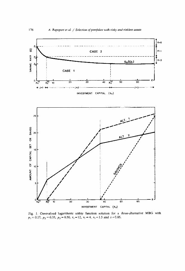
Fig. 1. Generalized logarithmic utility function solution for a three-alternative MBG with p, =0.17, pz=0.33, p3=0.50, r, =12, t-,=4, r,=1.5 and s=1.05.
A. Rapoport et al. / Selection of portfolios with risky and riskless assets 111
If xii) I x, < xLj+‘), the optimal amount bet on alternative i, y&, is given by
P. Yiyn = gxn + Pi ri Qj - Pj
a” if i=l,..., j / ri Pj
=0 if i=j+l,...,m,
and the amount allocated to the risk-free (savings) asset is
w*=o. n
Case 2. If s 2 S,(GL), Case 2 obtains and the decision follows. There exist m critical savings rates z, < z,,_~ < . . .
zk =Pkrk/(’ - pk +Pk%Qk), k=l,...,m-1.
(6)
(7)
policy is as < zr, where
(8)
If z k + 1 I s < zk, the optimal amount bet on alternative i is given by
Yiyn = Can + sxn) Pi’i-‘(‘-Pk+PiriQk> if i=l
(1 - SQ/c)SC ,---,
k
=0 if i=k+l,...,m,
and the optimal amount of capital saved is specified by
w,* = %1(1 - pk> + %bQk - pk>
S(l-@k) .
(9)
(10)
Eq. (6) shows that the predicted portfolio (Y&, J$, . . . , y,*,,) de- pends on the parameter a, and may consequently vary from trial to trial even if the investment capital x, is the same. Similarly for Case 2, eqs. (9) and (10) allow the portfolio to change from trial to trial as a function of a,. Despite this variation, certain parameter-free predict- ions may be derived for both Cases 1 and 2.
Denote the proportion of capital wagered on alternative i by ui,n = JJ~,/x, and the proportion of capital saved by u, = w,/x,. Although it is generally not the case, in all of our six experimental conditions m = 3, pIrIQj - Pj 2 0, p2r2Qj - PI I 0, and p3r3Qj - Pi I 0. There-

178 A. Rapoport et al. / Selection of portfolios with risky and riskless assets
fore, if Case 1 obtains, eq. (6) implies that r+ >pl/Pj, u2,n I~,/P~,
and ~3,~ s ~4 P regardless of the values of a, and x,. j If Case 2 obtains, eq. (9) states that zero bets should be wagered on
the risky alternatives k + 1,. . . , m, regardless of the values of a,, and x,. Another observation concerns eq. (10). Dividing both sides of (10) by X, and rearranging terms, we obtain
v,* = I-Pk a, sQ,c - pk
l-,sQ, +x,‘s(l-~(2~)’
Although it is in general not the case, in all of our six experimental groups Pk > sQk and 1 z=- se,. Therefore, regardless of the values of ~1, and x,, eq. (10) implies that u,* may not exceed the ratio (1 - P,)/(l
- sQk)- Another observation from (9) is that the ratio of wagers on alterna-
tives g and h, assuming that g, h I k, is a constant. Denoting this ratio by Rgh,n, we obtain
*
R" Y&n rh P& - ~(1 - fi + pgrgQk)]
gh,n = - = 1
Y&l rg[Phrh-S(l -&+PGlzQ/z)] ’
g, h I k. (11)
Combing the observations above, three predictions hold for each trial n. They involve inequalities which do not depend on either a or x, but only on the parameters of the MBG:
GLl. If Case 1 obtains,
Ul,n 2 Pl/P2 7 u2,n 5 p/P2 and ~3,~ 5 PU%
GL2. If Case 2 obtains,
u, 5 (1 -P&(1 - sQk) and
u~,~ 2 [ pirj - sfl -Pk+piriQk)]/(l -.~Q,)ri if i=l,..., k
=0 if i=k+l,...,m.
GL3. (Separation property) If Case 2 obtains, the ratio of the wagers on any two risky alternatives g and h is given by R&, in (11).

A. Rapoport et al. / Selection of portfolios with risky and riskless assets 119
Example. Consider a 3-alternative MBG with parameters p, = 0.17, p2 = 0.33, p3 = 0.50, r, = 12, r, = 4, r, = 1.5 and s = 1.05. Fig. 1 dis- plays the decision policy for a GL utility function with a, = 132. The values of x(l) = 0, x4’ = 6, and x, (3) = 44 are presented on the horizon- tal axis of he upper panel, whereas the critical savings rates zi = 2.04, z2 = 1.4043, and z3 = 1.0 are shown on the vertical axis. The function S,(GL) decreases in wealth from 2.04 when x, = xi” to 1.0 when x = xp’. If X” > x, ) (3) S (GL) = 1 always. Because z3 I s < z2, k = 2 if &se 2 obtains. Settin; S,(GL) = s = 1.05 and solving for x, (for a, = 132) yields x, = 37.715. Thus, as shown in fig. 1, a subject should allocate a positive fraction of his or her wealth to savings if x, 2 37.715 (Case 2) and nothing otherwise (Case 1).
The linear relations between yjTn and x, are displayed on the lower panel of fig. 1. If 0 I x, I 6, the entire investment capital should be wagered on alternative 1, if 6 5 x, I 37.715, the capital should be divided between the first two risky alternatives, and once the capital exceeds 37.715, it should be divided between the first two risky assets and the safe asset. No capital should ever be wagered on alternative 3 (which obtains with probability 0.50). With k = 2, we obtain for prediction GL2, u,, I 0.7692, qn 2 0.1027, u2+ 2 0.1281, and u3,n = 0. Prediction GL3 yields ~~~,/yi,~ = 1.247.
The NE utility model
The NE utility function has the form
U(X) = -exp( -a,x,), a, > 0.
The subject’s objective is maximization of the expected utility of immediate return
WXn+l )] = ,glpi [ _ e-%PJ,,“+sq (12)
subject to the usual constraints for the MBG. The decision policy which maximizes (12) is similar in form to the one prescribed by the GL model, falling again in one of two cases depending on s and x, (Funk et al. 1979). For each trial n, define the function
S,(NE)=Xn/[XnQ,+un(l-Pi)],

180 A. Rapoport et al. / Selection of portfolios with risky and riskless assets
where P, and Q j are defined as before, A, is given by
hl= exp $, ,F 1 i
m 1 -ln(W,4J -x,
J , 1 anri Ii >
and j is determined from the Case 1 solution below.
Case 1. If s < S,(NE), Case 1 obtains and the decision policy is as follows. There exist m + 1 critical investment capital values xij-l) such that
O=x@f<xpc .*. <,p, n where
xw-l) = n -rjQjKj(j) if j=l,...,m
=M if j=m+l, and
K,(j)=Ih
anr, i=l,..., j; j=l,..., m.
i=l
If xfjF1) < x, I xij), the optimal bet on alternative i is given by ”
yj~n=Kj(j)+x" riQj
if i= l,..., j
=0 if i=j+l,...,m, (13)
and the amount allocated to savings is
w*=o. n 04) Case 2. If s 2 ,S,,(NE), Case 2 obtains and the decision policy is as follows. There exist m critical values of the saving rate z, < z,_i < . . . c z1 as defined in (8). If zk+r 2 s < zk, the optimal amount wagered on alternative i is given by
Yif = &In (l-sQ/c)P;C if i=l
so- J-2 1 ,--*, k
n f
=0 if i=k+l,...,m, 05)

A. Rapoport et al. / Selection of portfolios with risky and riskless assets 181
and the amount of investment capital allocated to the safe asset is specified by
wn*=x,- Cl- SQk )Piri 1 s(l-P,) . (16)
Although upper or lower limits on yiyn in Case 1 may be derived from (13) they constitute very weak predictions which are not worth testing. However, as in the GL model above, the initial savings rates zk are time independent. Therefore, when Case 2 obtains, two predictions are derived, not depending on either a or x:
NEl. If Case 2 obtains, ui,n = 0 if i = k + 1,. . . , m.
NE2. (Separation property). If Case 2 obtains, the ratio of the wager on any two risky alternatives g and h (g, h I k) is given by (see eq. 15):
Y& R& = - =
r,ln[(l - sQd~,@(l- P,)] Y& @d(l- ~Q,)P,G/s(~ - &>I .
(17)
A comparison of models GL and NE shows that prediction NE1 is subsumed under GL2. However, predictions GL3 and NE2 differ from each other allowing a competitive test.
Example. Consider the same 3-alternative MBG as above with p1 = 0.17, p2 = 0.33, p3 = 0.50, r, = 12, r, = 4, r, = 1.5, and s = 1.05. For a NE utility function with parameter a = l/200, the initial capital levels are x(O) = 0, xi’) = 7.255, and x, (2) = 44 943. The initial savings rates are . zi = ;.04, z2 = 1.4043, and z3 = 1.0 as before. If Case 2 obtains, k = 2. Hence, prediction NE1 yields u~,~ = 0 and prediction NE2 yields
Y2Tn/Y& = I-591.
4. Test of the models
Method
MBG was originally constructed as a self-paced, computer-con- trolled, multi-stage portfolio selection game. The subjects in the six

182 A. Rapoport et al. / Selection of portfolios with risky and riskless assets
experimental groups were male and female students from the Univer- sity of Haifa in fsrael or the University of North Carolina at Chapel Hill, who volunteered to participate in the experiment for monetary reward. Each subject participated individually in seven (condition 2), four (conditions 1 and 3), or six (conditions 4, 5, and 6) sessions, each of which lasted between 45 and 100 minutes. Two to seven days separated consecutive sessions. Subjects received monetary payoff con- tingent on their performance by converting xN+r from points to money. The mean gain per session over all six conditions was about $8 with a few subjects earning as much as $30 per hour.
Table I summarizes information about the game parameters, number of subjects, number of sessions, and maximum number of trials by
Table 1 Summary of information for the six experimental conditions. a
Savings rate Return rates
Eaual Unequal
Favorable Condition 1
p1- 0.50, p2 = 0.33, ps = 0.17 r, = l-2 = ij = 3, s = 1.08 x1 =loo Number of Subjects - 14 Number of Sessions = 4 T-400
Condition d
p1 = 0.17, p2 = 0.33, p3 = a.50
r, =12, ?=4, !-,=X5, s-1.05 X,=100 Number of Subjects = 6 Number of Sessions = 6 T=900
EWSI
Condition 2
p1 = 0.50, p2 = 0.33. p3 = a.17
rl=r~=r~=3tS=1.0
Xl==l(lD Number of Subjects = 6 Number of Sessions = 7 T=MO
Condition 5
p1 = 0.17, p2 = 0.33, p3 - 0.50
r1=12, r*=4, r,=lS, s=l,O X,=laO Number of Subjects = 6 Number of Sessions = 7 T=9OO
Unfavorable Condition 3 Condition 6
pi = 0.50, p2 = 0.33, p3 = 0.17 PI = 0.17, pz = 0.33, p3 = OS0
8) = r, = rx = 2.4, s = 0.86 r, = 12, r, = 4, rs = 1.5, s = 0.95
x1 = 3000 x,=200
Number of Subjects = 14 Number of Subjects = 6 Number of Sessions = 4 Number of Sessions = 6 T=400 T=9#
a T equals the matimm number of trials per subject over all the sessions, provided ail games terminated with no bankruptcy and the ceiling on xnfl was never exceeded.
A. Rapoport et al. / Selection of portfolios with risky and riskless assets 183
condition. Detailed information can be found in Funk et al. (1979) for condition 2, Rapoport (1984) for conditions 1 and 3, and Rapoport et al. (1985) for conditions 4, 5, and 6. Table 1 shows that conditions 1 through 6 form a 2 x 3 return rate by savings rate factorial design. Conditions 1, 2, and 3 have equal return rates whereas in conditions 4, 5, and 6 the return rates are negatively correlated with the outcome probabilities. In terms of the savings rate, conditions 1 and 4 are favorable with s > 1, conditions 3 and 6 are unfavorable with s < 1, and conditions 2 and 5 are euen with x = 1.
Generally increasing their initial capital (xi = 100) under the favora- ble investment conditions, the subjects in conditions 1 and 4, and to a lesser extent in the conditions 2 and 5, can be assumed to mostly aspire to maximize gain. In contrast, typically watching their initial capital (x1 = 3000 or 200) rapidly dwindling over trials under the unfavorable investment conditions, the subjects in condition 3 and to a lesser extent in condition 6 can be assumed to mostly aspire to minimize loss. Although formally equivalent, the two criteria of maximization of gain and minimization of loss are phenomenologically distinct and may cause different patterns of decision behavior (Kahneman and Tversky 1979).
In all the six conditions each session included six independent games that differed from one another in the value of N. N ranged from 9 to 36 to ensure that the subject could not anticipate the end of the game. The maximum number of trials per session was 120 for condition 2,100 for conditions 1 and 6, and 150 for conditions 3, 4, and 5. Each game had an undisclosed ceiling to control for experimental expenses. This maximum limit on x, + 1 varied from one session to another to alleviate suspicion on the part of the subjects. Subjects seldom exceeded the maximum limit.
Written instructions were distributed to the subjects stating that the experiment was conducted ‘to learn more about how people make decisions’. The outcome probabilities were explained in terms of a wheel of fortune divided into areas whose sizes corresponded to the pi’s or in terms of drawing marbles from a box with replacement. Subjects were further instructed that N would vary from game to game in a random way, that pi, r, and s would remain unchanged during the entire experiment, that successive trials within games were indepen- dent, and that their objective was to ‘earn as much money as possible’ in each game.
184 A. Rapoport et al. / Selection ofportfolios with risky and riskless assets
Results
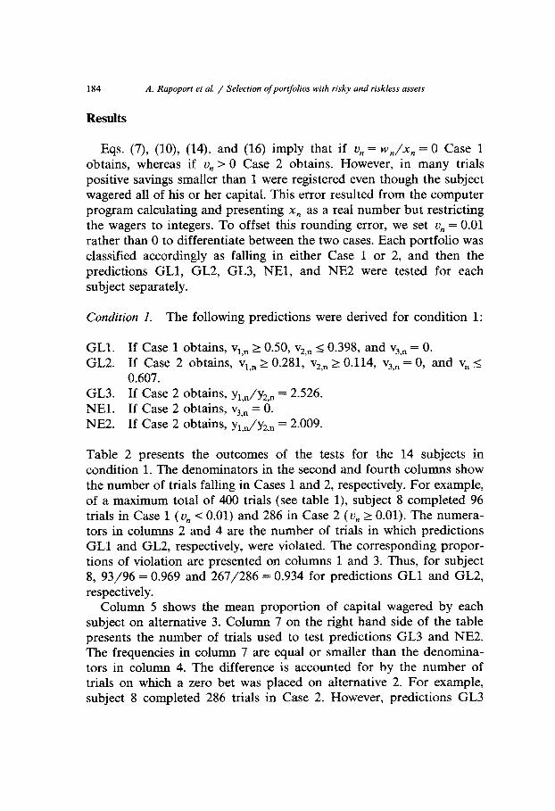
Eqs. (7), (lo), (14), and (16) imply that if u, = w,/x, = 0 Case 1 obtains, whereas if u, > 0 Case 2 obtains. However, in many trials positive savings smaller than 1 were registered even though the subject wagered all of his or her capital. This error resulted from the computer program calculating and presenting X, as a real number but restricting the wagers to integers. To offset this rounding error, we set u, = 0.01 rather than 0 to differentiate between the two cases, Each portfolio was classified accordingly as falling in either Case 1 or 2, and then the predictions GLl, GL2, GL3, NEl, and NE2 were tested for each subject separately.
Condition 1. The following predictions were derived for condition 1:
GLl. If Case 1 obtains, 2 0.50, I 0.398, and = 0. vi,* v,,~ v,,~ GL2. If Case 2 obtains, > 0.281, 2 0.114, = 0, and v,,~ v,,~ v,,~ v, I
0.607. GL3. If Case 2 obtains, y,,.,/y,,, = 2.526. NEl. If Case 2 obtains, v,,~ = 0. NE2. If Case 2 obtains, ~i,~/y~,~ = 2.009.
Table 2 presents the outcomes of the tests for the 14 subjects in condition 1. The denominators in the second and fourth columns show the number of trials falling in Cases 1 and 2, respectively. For example, of a maximum total of 400 trials (see table l), subject 8 completed 96 trials in Case 1 (u, < 0.01) and 286 in Case 2 (u, 2 0.01). The numera- tors in columns 2 and 4 are the number of trials in which predictions GLl and GL2, respectively, were violated. The corresponding propor- tions of violation are presented on columns 1 and 3. Thus, for subject 8, 93/96 = 0.969 and 267/286 = 0.934 for predictions GLl and GL2, respectively.
Column 5 shows the mean proportion of capital wagered by each subject on alternative 3. Colurrm 7 on the right hand side of the table presents the number of trials used to test predictions GL3 and NE2. The frequencies in column 7 are equal or smaller than the denomina- tors in column 4. The difference is accounted for by the number of trials on which a zero bet was placed on alternative 2. For example, subject 8 completed 286 trials in Case 2. However, predictions GL3
A. Rapoport et al. / Selection of portfolios with risky and riskless assets 185
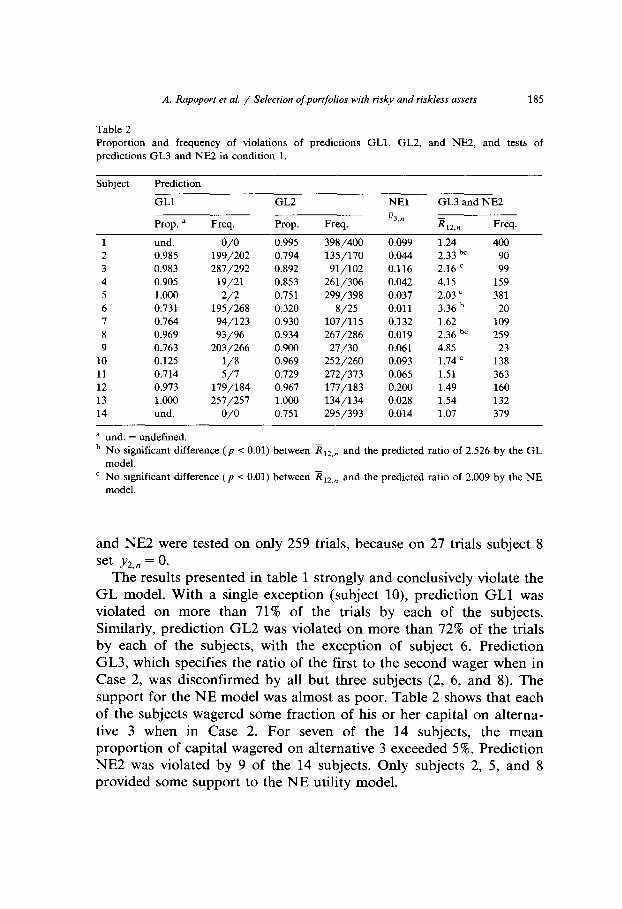
Table 2 Proportion and frequency of violations of predictions GLI, GL2, and NE2, and tests of predictions GL3 and NE2 in condition 1.
Subject
1 2 3 4 5 6 7 8 9
10 11 12 13 14
Prediction
GLl GL2 NE1 GL3 and NE2
Prop. a Freq. Prop. Freq. %n
R 12.n Freq.
und. O/O 0.995 398/400 0.099 1.24 400 0.985 199/202 0.194 135/170 0.044 2.33 bc 90 0.983 281/292 0.892 91/102 0.116 2.16 ’ 99
0.905 19/21 0.853 261/306 0.042 4.15 159 1.000 2/2 0.751 299/398 0.037 2.03 = 381
0.731 195/268 0.320 8/25 0.011 3.36 b 20 0.764 94/123 0.930 107/115 0.132 1.62 109
0.969 93/96 0.934 267/286 0.019 2.36 ” 259 0.763 203/266 0.900 27/30 0.061 4.85 23 0.125 L/8 0.969 252/260 0.093 1.74 c 138 0.714 5/7 0.729 272/373 0.065 1.51 363 0.973 179/184 0.967 177/183 0.200 1.49 160 1.000 257/257 1.000 134/134 0.028 1.54 132 und. O/O 0.751 295/393 0.014 1.07 379
’ und. = undefined. b No significant difference ( p i 0.01) between R,,,, and the predicted ratio of 2.526 by the GL
model. ’ No significant difference (p -z 0.01) between Et,,, and the predicted ratio of 2.009 by the NE
model.
and NE2 were tested on only 259 trials, because on 27 trials subject 8 set y2,n = 0.
The results presented in table 1 strongly and conclusively violate the GL model. With a single exception (subject lo), prediction GLl was violated on more than 71% of the trials by each of the subjects. Similarly, prediction GL2 was violated on more than 72% of the trials by each of the subjects, with the exception of subject 6. Prediction GL3, which specifies the ratio of the first to the second wager when in Case 2, was disconfirmed by all but three subjects (2, 6, and 8). The support for the NE model was almost as poor. Table 2 shows that each of the subjects wagered some fraction of his or her capital on altema- tive 3 when in Case 2. For seven of the 14 subjects, the mean proportion of capital wagered on alternative 3 exceeded 5%. Prediction NE2 was violated by 9 of the 14 subjects. Only subjects 2, 5, and 8 provided some support to the NE utility model.
186 A. Rapoport et al. / Selection of portfolios with risky and riskless assets
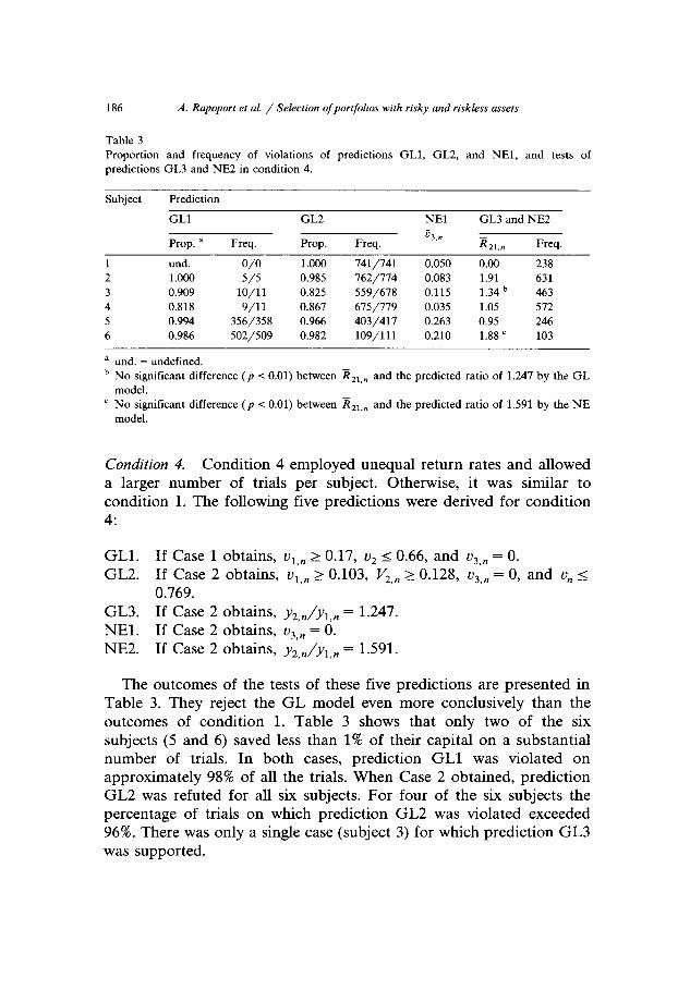
Table 3
Proportion and frequency of violations of predictions GLl, GL2, and NEl, and tests of
predictions GL3 and NE2 in condition 4.
Subject
1
2
3
4
5
6
Prediction
GLl GL2 NE1 GL3 and NE2
Prop. a Freq. Prop. Freq. 83,”
R 21,” Freq.
und. O/O 1.000 741/741 0.050 0.00 238
1.000 5/5 0.985 x2/174 0.083 1.91 631
0.909 lO/ll 0.825 559/678 0.115 1.34 b 463
0.818 9/11 0.867 615/119 0.035 1.05 572
0.994 356/358 0.966 403/417 0.263 0.95 246
0.986 502/509 0.982 109/111 0.210 1.88 = 103
a turd. = undefined.
b No significant difference (p < 0.01) between x,,,, and the predicted ratio of 1.247 by the GL
model.
’ No significant difference (p < 0.01) between ii 21.n and the predicted ratio of 1.591 by the NE
model.
Condition 4. Condition 4 employed unequal return rates and allowed a larger number of trials per subject. Otherwise, it was similar to condition 1. The following five predictions were derived for condition 4:
GLl. If Case 1 obtains, ~i,~ 2 0.17, I 0.66, and u2 u3+ = 0. GL2. If Case 2 obtains, ~r,~ 2 0.103, V,,, 2 0.128, u3,n = 0, and u,, I
0.769. GL3. If Case 2 obtains, ~Qyr,~ = 1.247. NEl. If Case 2 obtains, u3,n = 0. NE2. If Case 2 obtains, ~+./yr,~ = 1.591.
The outcomes of the tests of these five predictions are presented in Table 3. They reject the GL model even more conclusively than the outcomes of condition 1. Table 3 shows that only two of the six subjects (5 and 6) saved less than 1% of their capital on a substantial number of trials. In both cases, prediction GLl was violated on approximately 98% of all the trials. When Case 2 obtained, prediction GL2 was refuted for all six subjects. For four of the six subjects the percentage of trials on which prediction GL2 was violated exceeded 96%. There was only a single case (subject 3) for which prediction CL3 was supported.
A. Rapoport et al. / Selection ojportjoiios with risky and riskless assets 187
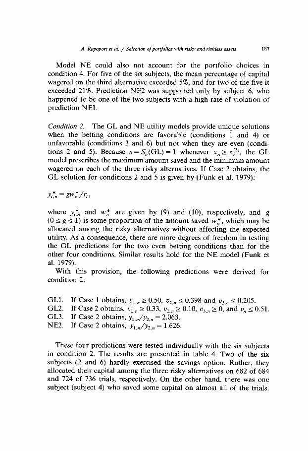
Model NE could also not account for the portfolio choices in condition 4. For five of the six subjects, the mean percentage of capital wagered on the third alternative exceeded 5%, and for two of the five it exceeded 21%. Prediction NE2 was supported only by subject 6, who happened to be one of the two subjects with a high rate of violation of prediction NEl.
Condition 2. The GL and NE utility models provide unique solutions when the betting conditions are favorable (conditions 1 and 4) or unfavorable (conditions 3 and 6) but not when they are even (condi- tions 2 and 5). Because s = S,(GL) = 1 whenever x, 2 xk3), the GL model prescribes the maximum amount saved and the minimum amount wagered on each of the three risky alternatives. If Case 2 obtains, the GL solution for conditions 2 and 5 is given by (Funk et al. 1979):
where yiFn and w,* are given by (9) and (lo), respectively, and g (0 I g < 1) is some proportion of the amount saved wz, which may be allocated among the risky alternatives without affecting the expected utility. As a consequence, there are more degrees of freedom in testing the GL predictions for the two even betting conditions than for the other four conditions. Similar results hold for the NE model (Funk et al. 1979).
With this provision, the following predictions were derived for condition 2:
GLl. If Case 1 obtains, u 2 0.50, i n u2 n I 0.398 and 03,n < 0.205. GL2. If Case 2 obtains, u 12 0.33, 1 u2 u3 n I, 2 0.10, 2 GL3. If Case 2 obtains, y;,,/yz,, = 2.663. ’
0, and I 0.51. u,
NE2. If Case 2 obtains, yiJy2,n = 1.626.
These four predictions were tested individually with the six subjects in condition 2. The results are presented in table 4. Two of the six subjects (2 and 6) hardly exercised the savings option. Rather, they allocated their capital among the three risky alternatives on 682 of 684 and 724 of 736 trials, respectively. On the other hand, there was one subject (subject 4) who saved some capital on almost all of the trials.
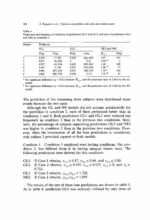
188 A. Rapoport et al. / Selection of portfolios with risky and riskless assets
Table 4 Proportion and frequency of violations of predictions GLl and GL2, and tests of predictions GL3
and NE2 in condition 2.
Subject
1
2
3
4
5
6
Prediction
GLl GL2 GL3 and NE2
Prop. Freq. Prop. Freq. R 12.” Freq.
0.250 17/68 0.914 602/659 3.57 551 0.111 76/682 0 O/2 2.68 ab 2 0.557 69/124 0.638 429/663 1.28 549 0.367 11/30 0.932 576/618 1.96 ab 77 0.491 107/218 0.661 144/218 1.51 b 160 0.801 580/724 0.250 3/12 1.51 ab 12
a No significant difference (p < 0.01) between RI,,, and the predicted ratio of 2.063 by the GL
model. b No significant difference (p < 0.01) between RI,,, and the predicted ratio of 1.626 by the NE
model.
The portfolios of the remaining three subjects were distributed more evenly between the two cases.
Although the GL and NE models did not account satisfactorily for the portfolios in condition 2, each of them performed better than in conditions 1 and 4. Both predictions GLl and GL2 were violated less frequently in condition 2 than in the previous two conditions. Simi- larly, the percentage of subjects supporting predictions GL3 and NE2 was higher in condition 2 than in the previous two conditions. How- ever, when the intersection of all the four predictions is considered, only subject 2 provided support to both models.
Condition 5. Condition 5 employed even betting conditions, like con- dition 2, but differed from it in having unequal return rates. The following predictions were derived for this condition:
GLl. If Case 1 obtains, ~r,~ u2,n 2 0.17, I 0.66, and ~9~ I 1.00. GL2. If Case 2 obtains, ~i,~ u2,n 2 0.115, 2 0.153, 2 0, and u3,n u,, I
0.732. GL3. If Case 2 obtains, y2,,/yi,, = 1.326. NE2. If Case 2 obtains, JQJ+~ = 1.695.
The results of the test of these four predictions are shown in table 5. As in table 4, prediction GLl was seriously violated by only three of
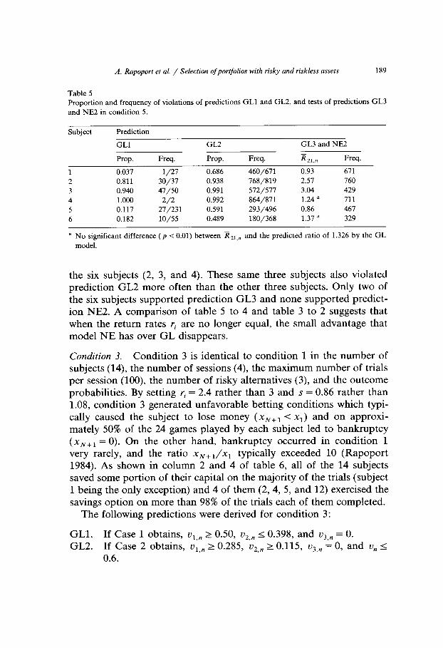
A. Rapoport et al. / Selection of portfolios with risky and riskless assets 189
Table 5 Proportion and frequency of violations of predictions GLl and GL2, and tests of predictions GL3
and NE2 in condition 5.
Subject
1
2 3 4
5
6
Prediction
GLl GL2 GL3 and NE2
Prop. Freq. Prop. Freq. w 21.” Freq.
0.037 l/27 0.686 460/671 0.93 671 0.811 30/37 0.938 768/819 2.57 760 0.940 47/50 0.991 572/517 3.04 429 1.000 2/2 0.992 864/871 1.24 a 711 0.117 27/231 0.591 293/496 0.86 467 0.182 10/55 0.489 180/368 1.37 a 329
a No significant difference (p < 0.01) between x 21.n and the predicted ratio of 1.326 by the GL
model.
the six subjects (2, 3, and 4). These same three subjects also violated prediction GL2 more often than the other three subjects. Only two of the six subjects supported prediction GL3 and none supported predict- ion NE2. A comparison of table 5 to 4 and table 3 to 2 suggests that when the return rates ri are no longer equal, the small advantage that model NE has over GL disappears.
Condition 3. Condition 3 is identical to condition 1 in the number of subjects (14), the number of sessions (4), the maximum number of trials per session (loo), the number of risky alternatives (3), and the outcome probabilities. By setting r, = 2.4 rather than 3 and s = 0.86 rather than 1.08, condition 3 generated unfavorable betting conditions which typi- cally caused the subject to lose money ( xN+i < xi) and on approxi- mately 50% of the 24 games played by each subject led to bankruptcy
(x N+l = 0). On the other hand, bankruptcy occurred in condition 1 very rarely, and the ratio xN+i /xi typically exceeded 10 (Rapoport 1984). As shown in column 2 and 4 of table 6, all of the 14 subjects saved some portion of their capital on the majority of the trials (subject 1 being the only exception) and 4 of them (2, 4, 5, and 12) exercised the savings option on more than 98% of the trials each of them completed.
The following predictions were derived for condition 3:
GLl. If Case 1 obtains, ~i,~ 2 0.50, .v~,~ I 0.398, and u~,~ = 0. GL2. If Case 2 obtains, ~i,~ 2 0.285, u*,~ 2 0.115, u~,~ = 0, and u,, I
0.6.
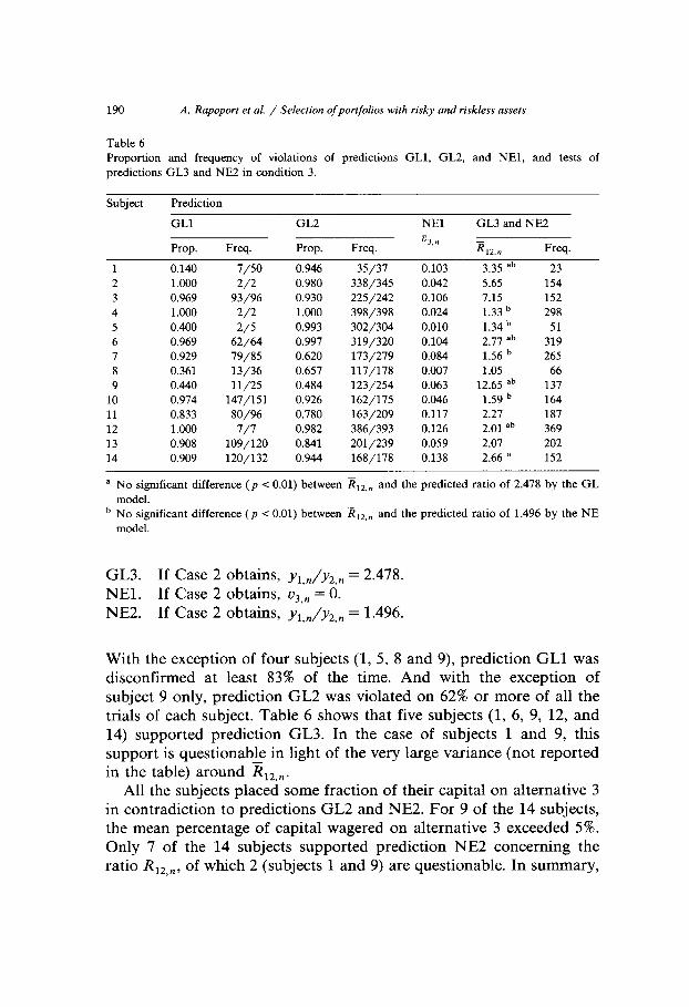
190 A. Rapoport et al. / Selection of portfolios with risky and riskless assets
Table 6 Proportion and frequency of violations of predictions GLl, GL2, and NEl, and tests of predictions GL3 and NE2 in condition 3.
Subject Prediction
GLl GL2 NE1 GL3 and NE2
1 2 3 4 5 6 7 8 9
10 11 12 13 14
Prop.
0.140
Freq.
7/50
Prop.
0.946
Freq.
35/37
~3.n R 12.” Freq.
0.103 3.35 ab 23 1.000 2j2 0.980 338;345 0.042 5.65 154 0.969 93/96 0.930 225/242 0.106 7.15 152 1.000 2/2 1.000 398/398 0.024 1.33 b 298 0.400 215 0.993 302/304 0.010 1.34 b 51 0.969 62/64 0.997 319/320 0.104 2.77 ab 319 0.929 79/85 0.620 173/279 0.084 1.56 b 265 0.361 13/36 0.657 117/178 0.007 1.05 66 0.440 11/25 0.484 123/254 0.063 12.65 ab 137 0.974 147/151 0.926 162/175 0.046 1.59 b 164 0.833 80/96 0.780 163/209 0.117 2.27 187 1.000 7/7 0.982 386/393 0.126 2.01 ab 369 0.908 109/120 0.841 201/239 0.059 2.07 202 0.909 120/132 0.944 168/178 0.138 2.66 = 152
a No significant difference (p < 0.01) between XII,+ and the predicted ratio of 2.478 by the GL model.
b No significant difference (p < 0.01) between RI,,, and the predicted ratio of 1.496 by the NE model.
GL3. If Case 2 obtains, y1,/y2,. = 2.478. NEl. If Case 2 obtains, u3,n = 0. NE2. If Case 2 obtains, yiJy2,. = 1.496.
With the exception of four subjects (1, 5, 8 and 9), prediction GLl was disconfirmed at least 83% of the time. And with the exception of subject 9 only, prediction GL2 was violated on 62% or more of all the trials of each subject. Table 6 shows that five subjects (1, 6, 9, 12, and 14) supported prediction GL3. In the case of subjects 1 and 9, this support is questionable in light of the very large variance (not reported in the table) around R12,n.
All the subjects placed some fraction of their capital on alternative 3 in contradiction to predictions GL2 and NE2. For 9 of the 14 subjects, the mean percentage of capital wagered on alternative 3 exceeded 5%. Only 7 of the 14 subjects supported prediction NE2 concerning the ratio R12,n, of which 2 (subjects 1 and 9) are questionable. In summary,
A. Rapoport et al. / Selection of portfolios with risky and riskless assets 191
the difference between conditions 1 and 3 hardly changed the poor fit of the GL and NE models. None of the subjects supported the GL model, and the results of only three subjects (4, 5, and 10) were compatible with the predictions of the NE model.
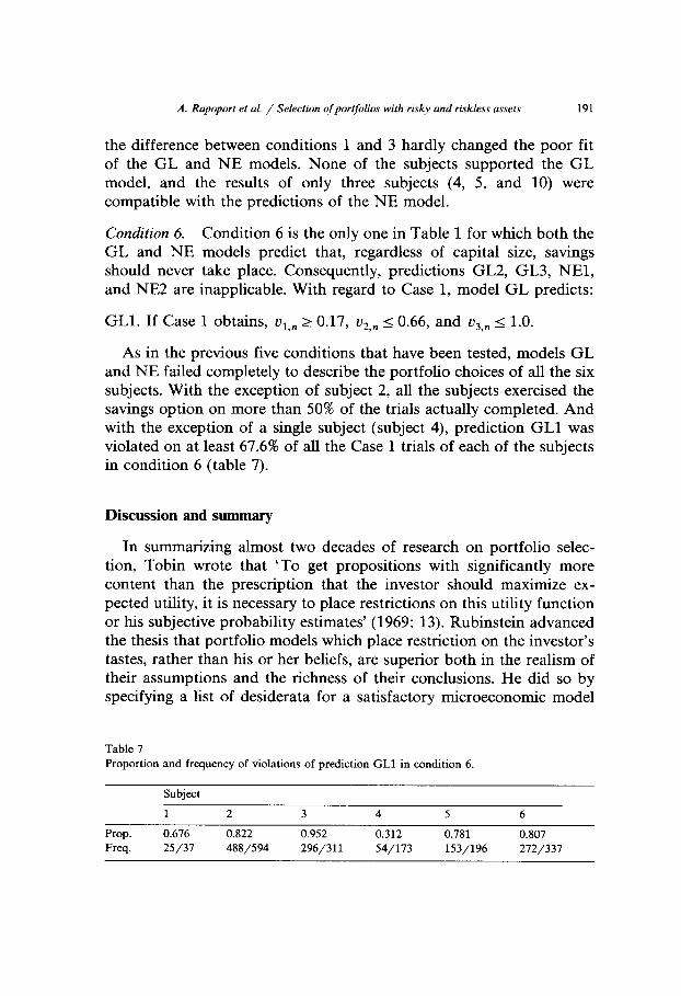
Condition 6. Condition 6 is the only one in Table 1 for which both the GL and NE models predict that, regardless of capital size, savings should never take place. Consequently, predictions GL2, GL3, NEl, and NE2 are inapplicable. With regard to Case 1, model GL predicts:
GLl. If Case 1 obtams, ~i,~ _ > 0.17, u*,~ I 0.66, and v~,~ I 1.0.
As in the previous five conditions that have been tested, models GL and NE failed completely to describe the portfolio choices of all the six subjects. With the exception of subject 2, all the subjects exercised the savings option on more than 50% of the trials actually completed. And with the exception of a single subject (subject 4), prediction GLl was violated on at least 67.6% of all the Case 1 trials of each of the subjects in condition 6 (table 7).
Discussion and summary
In summarizing almost two decades of research on portfolio selec- tion, Tobin wrote that ‘To get propositions with significantly more content than the prescription that the investor should maximize ex- pected utility, it is necessary to place restrictions on this utility function or his subjective probability estimates’ (1969: 13). Rubinstein advanced the thesis that portfolio models which place restriction on the investor’s tastes, rather than his or her beliefs, are superior both in the realism of their assumptions and the richness of their conclusions. He did so by specifying a list of desiderata for a satisfactory microeconomic model
Table 7 Proportion and frequency of violations of prediction GLl in condition 6
Subject
1 2 3 4 5 6
Prop. 0.676 0.822 0.952 0.312 0.781 0.807 Freq. 25/37 488/594 296/311 54/173 153/196 272/337
192 A. Rapoport et al. / Selection of portfolios with risky and riskless assets
of financial markets and showed that the GL is the only model which satisfies them. On particular relevance to our MBG studies is the observation that when the single parameter of the GL model is zero or is very small relative to the investor’s capital, the investor would follow the famous Bernoulli-Laplace hypothesis about the marginal utility of income as well as obey the Weber-Fechner law of psychophysics that the marginal impact of a stimulus is inversely related to the stimulus’ intensity.
Although it does not satisfy all the desiderata proposed by Rubin- stein, the NE model satisfies most of them as well as most of the conclusions which have been proposed by Rubinstein to characterize a satisfactory model of financial markets. Also, as noted above, the GL and NE are the only single-parameter utility models which belong to the HARA or linear risk tolerance class of tastes, the significance of which has been noted by Cass and Stiglitz (1970).
In six different groups containing undergraduate and graduate stu- dents from two continents, attempts were made to achieve suitable experimental conditions for testing the descriptive power of the two models. The number of risky alternatives in MBG, outcome probabili- ties, return rates, and savings rate were kept unaltered during the experiment in order to simplify the cognitive demands on the subject without rendering the task too obvious. To compensate for lack of previous experience with portfolio selection as well as examine learning effects, each subject was run for a maximum total of 400 to 900 trials divided into 24 to 30 games of an unknown duration, which were administered within a period of 2 of 3 weeks. Motivation was elicited and continuously maintained by presenting portfolio choices as gam- bles and paying the subject nontrivial amounts of money contingent on his or her performance. Moreover, we formulated and tested a very weak version of the two models, which allows not only for heterogene- ity of subjects but also for trial-to-trial variation in the choices of the same subject. It was hoped that if this weak version were proved satisfactory, accounting for the major characteristics of the subjects’ portfolio choices, the parameter a,, would be estimated and the varia- bles which cause its variation (e.g., capital size, trial number within game, previous wins and losses) would be determined by regression techniques.
This hope was not realized as the experimental results refuted both models consistently and overwhelmingly. Because the factorial design

A. Rapopori et al. / Selection of portfolios with risky and riskless assets 193
was incomplete, with condition 6 providing no predictions for Case 2, no attempt was made to test the effects of the two factors of betting conditions and return rates on the proportions of violation of the various predictions. Inspection of tables 2 through 7 suggests that the betting conditions (favorable, even, and unfavorable) had no discerna- ble effect of the proportions of violation but that both models were refuted more frequently when the return rates were unequal and negatively correlated with the outcome probabilities.
What implications do these negative findings have for subsequent attempts to formulate the regularities in portfolio selection reported in the MBG studies? One could, of course, adhere to the expected utility approach but investigate other utility functions. The generalized power utility model in eq. (4), which has two parameters that could be varied from trial to trial, is a natural candidate. Other expected utility models, which are psychologically interpretable and are consistent with the major findings of previous MBG studies regarding both absolute and proportional risk aversion, could also be examined. A second possibil- ity would be to develop and test models which restrict the investor’s beliefs such as the mean-variance model of Markowitz and some of its variations. A third possibility, which would seem consistent with the experimental findings on decision behavior under uncertainty that are well documented in the psychological literature (Hogarth 1981; Kahne- man, Slavic, and Tversky 1982; Slavic, Fischhoff, and Lichtenstein 1977), would be hybrid models which, rather than restricting either tastes or beliefs, restrict them both.
References
Cass, D. and J. Stightz, 1970. The structure of investor preferences and asset returns and
separability in portfolio allocation: A contribution to the pure theory of mutual funds. Journal
of Economic Theory 2, 122-160.
Elton, E.J. and M.J. Gruber, 1984. Modem portfolio theory and investment analysis (2nd ed.).
New York: Wiley.
Fishbum, P.C. and R.B. Porter, 1976. Optimal portfolios with one safe and one risky asset:
Effects of changes in rate of return and risk. Management Science 22, 1064-1073.
Funk, KG., A. Rapoport, and L.V. Jones, 1979. Investing capital on safe and risky alternatives:
An experimental study. Journal of Experimental Psychology: General 108,415~440. Gordon, M.J., G.E. Paradis, and C.H. Rourke, 1972. Experimental evidence on alternative
portfolio decision rules. American Economic Review 52, 107-118.
Hakansson, N.H., 1970. Optimal investment and consumption strategies under risk for a class of
utility functions. Econometrica 38, 587-607.

194 A. Rapoport et al. / Selection of portfolios with risky and riskless assets
Hakansson, N.H., 1971. Multi-period mean-variance analysis: Toward a general theory of portfolio choice. The Journal of Finance 26, 857-884.
Hakansson, N.H., 1974. Convergence to isoelastic utility and policy in multiperiod portfolio choice. Journal of Financial Economics 1,201-224.
Hogarth, R.M., 1981. Beyond discrete biases: Functional and dysfunctional aspects of judgmental heuristics. Psychological Bulletin 90, 197-217.
Kahneman, D., P. Slavic, and A. Tversky, eds., 1982. Judgement under uncertainty: Heuristics and biases. Cambridge: Cambridge University Press.
Kahneman, D. and A. Tversky, 1979. Prospect theory: An analysis of decision under risk. Econometrica 47, 263-291.
Kroll, Y., H. Levy and A. Rapoport, in press, a. Experimental tests of the mean-variance model for portfolio selection. Organizational Behavior and Human Decision Processes.
Kroll, Y., H. Levy, A. Rapoport in press, b. Experimental tests of the separation theorem and the capital asset pricing model. American Economic Review.
Levy, H. and M. Samat, 1984. Portfolio and investment selection: Theory and practice. New York: Wiley.
Mossin, J., 1968. Optimal multiperiod portfolio policies. Journal of Business 41, 215-229. Rapoport, A., 1970. Minimization of risk and maximization of expected utility in multistage
betting games. Acta Psychologica 34, 375-386. Rapoport, A., 1984. Effects of wealth on portfolios under various investment conditions. Acta
Psychologica 55, 31-51. Rapoport, A., S.G. Funk, J.R. Levinsohn, and L.V. Jones, 1977. How one gambles if one must:
Effects of differing return rates on multistage betting decisions. Journal of Mathematical Psychology 15, 169-198.
Rapoport, A., S.G. Funk, and R. Zwick, 1985. Risky and riskless choices in a multi-stage betting game with unequal returns. Unpublished manuscript.
Rapoport, A. and L.V. Jones, 1970. Gambling behavior in two-choice multistage betting games. Journal of Mathematical Psychology 7, 163-187.
Rapoport, A., L.V. Jones, and J.P. Kahan, 1970. Gambling behavior in multiple-choice betting games. Journal of Mathematical Psychology 7, 12-36.
Rubinstein, M., 1977. The strong case for the generalized logarithmic utility model as the premier model of financial markets. In: H. Levy and M. Samat (eds.), Financial decision making under uncertainty New York: Academic Press. pp. 11-62.
Slavic, P., B. Fischhoff, and S. Lichtenstein, 1977. Behavioral decision theory. Annual Review of Psychology 28, l-39.
Tobin, J., 1969. Comment on Borch and Feldstein. Review of Economic Studies 36, 13-14.