SELECTED PROBLEMS OF ELECTRONS CONFINED TO NANOSCALED SYSTEMS … · 2009-04-03 · Elisabeth Rogl...
63
Elisabeth Rogl SELECTED PROBLEMS OF ELECTRONS CONFINED TO NANOSCALED SYSTEMS Bachelor thesis Supervisor: Univ.-Prof. Ph.D. Peter Hadley Institute of Solid State Physics GRAZ UNIVERSITY OF TECHNOLOGY March 20, 2009 1
Transcript of SELECTED PROBLEMS OF ELECTRONS CONFINED TO NANOSCALED SYSTEMS … · 2009-04-03 · Elisabeth Rogl...
Elisabeth Rogl
SELECTED PROBLEMS OF ELECTRONSCONFINED TO NANOSCALED SYSTEMS
Bachelor thesis
Supervisor:Univ.-Prof. Ph.D. Peter Hadley
Institute of Solid State PhysicsGRAZ UNIVERSITY OF TECHNOLOGY
March 20, 2009
1
Contents
1 Introduction 2
2 Structure of calculation 32.1 Defining the dimension of the problem . . . . . . . . . . . . . . . 32.2 Finding the Solutions . . . . . . . . . . . . . . . . . . . . . . . . 32.3 Dispersion relation (DISP) . . . . . . . . . . . . . . . . . . . . . . 32.4 Denstity of states (DOS) . . . . . . . . . . . . . . . . . . . . . . . 6
2.4.1 0-dimensional DOS . . . . . . . . . . . . . . . . . . . . . . 92.4.2 1-dimensional DOS . . . . . . . . . . . . . . . . . . . . . . 92.4.3 2-dimensional DOS . . . . . . . . . . . . . . . . . . . . . . 132.4.4 3-dimensional DOS . . . . . . . . . . . . . . . . . . . . . . 15
3 Electrons confined to a square 173.1 Dispersion relation . . . . . . . . . . . . . . . . . . . . . . . . . . 203.2 Density of states . . . . . . . . . . . . . . . . . . . . . . . . . . . 20
4 Electrons confined to a rectangle 224.1 Dispersion relation . . . . . . . . . . . . . . . . . . . . . . . . . . 234.2 Density of states . . . . . . . . . . . . . . . . . . . . . . . . . . . 244.3 Program . . . . . . . . . . . . . . . . . . . . . . . . . . . . . . . . 26
5 Electrons confined to the surface of a torus 265.1 Finding Solutions . . . . . . . . . . . . . . . . . . . . . . . . . . . 265.2 Dispersion relation . . . . . . . . . . . . . . . . . . . . . . . . . . 315.3 Density of states . . . . . . . . . . . . . . . . . . . . . . . . . . . 335.4 Program . . . . . . . . . . . . . . . . . . . . . . . . . . . . . . . . 35
6 Electrons confined to the surface of a sphere 366.1 Background for radial symmetric problems . . . . . . . . . . . . . 376.2 Operators of angular momentum: . . . . . . . . . . . . . . . . . . 386.3 The orbital angular momentum operator L in real space: . . . . . 406.4 Dispersion relation . . . . . . . . . . . . . . . . . . . . . . . . . . 446.5 Density of states . . . . . . . . . . . . . . . . . . . . . . . . . . . 446.6 Program . . . . . . . . . . . . . . . . . . . . . . . . . . . . . . . . 47
7 Appendix 48
8 Literature 50
1
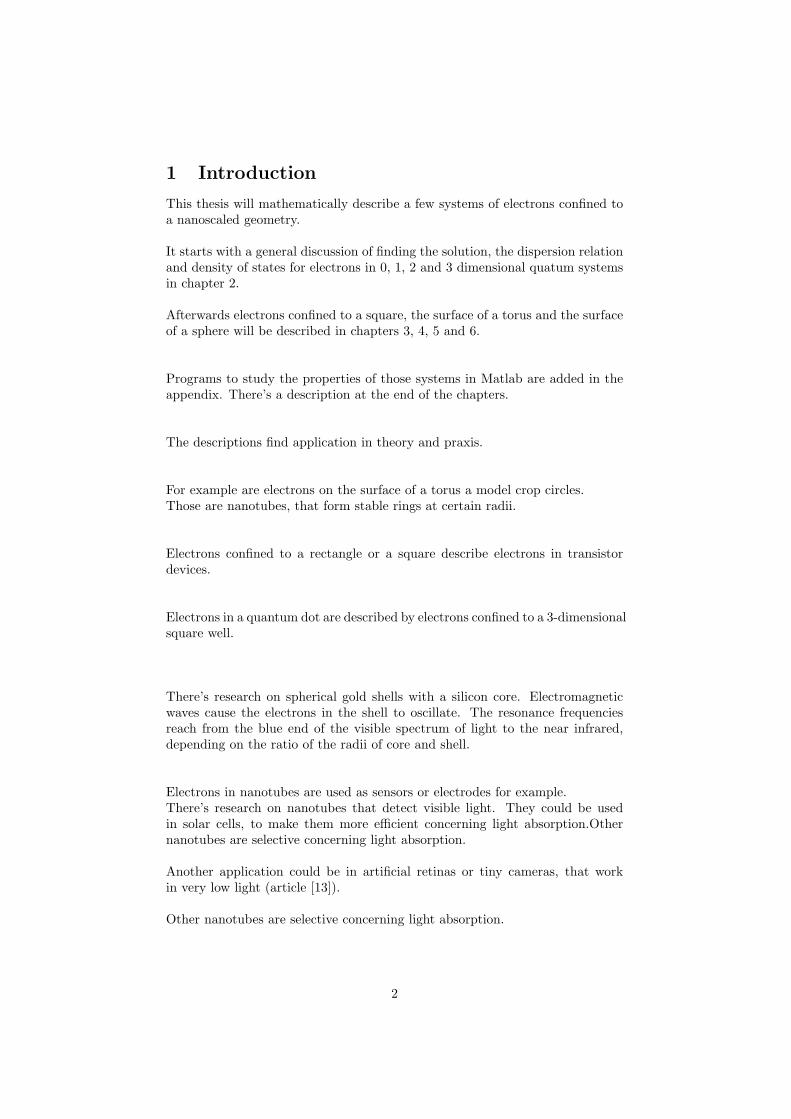
1 Introduction
This thesis will mathematically describe a few systems of electrons confined toa nanoscaled geometry.
It starts with a general discussion of finding the solution, the dispersion relationand density of states for electrons in 0, 1, 2 and 3 dimensional quatum systemsin chapter 2.
Afterwards electrons confined to a square, the surface of a torus and the surfaceof a sphere will be described in chapters 3, 4, 5 and 6.
Programs to study the properties of those systems in Matlab are added in theappendix. There’s a description at the end of the chapters.
The descriptions find application in theory and praxis.
For example are electrons on the surface of a torus a model crop circles.Those are nanotubes, that form stable rings at certain radii.
Electrons confined to a rectangle or a square describe electrons in transistordevices.
Electrons in a quantum dot are described by electrons confined to a 3-dimensionalsquare well.
There’s research on spherical gold shells with a silicon core. Electromagneticwaves cause the electrons in the shell to oscillate. The resonance frequenciesreach from the blue end of the visible spectrum of light to the near infrared,depending on the ratio of the radii of core and shell.
Electrons in nanotubes are used as sensors or electrodes for example.There’s research on nanotubes that detect visible light. They could be usedin solar cells, to make them more efficient concerning light absorption.Othernanotubes are selective concerning light absorption.
Another application could be in artificial retinas or tiny cameras, that workin very low light (article [13]).
Other nanotubes are selective concerning light absorption.
2
2 Structure of calculation
2.1 Defining the dimension of the problem
0 dimensional problem: the electrons are confined to a 3-dimensional quan-tum well (small cube or quantum dot). It’s motion is quantized in all directions.
1 dimensional problem: electrons confined to a quatum wire (f.e. poly-mers). The electrons are quasi free in one direction.
2 dimensional problem: electrons confined to a plane (f.e. in a transis-tor device).
3 dimensional problem: electrons in a bulk.
2.2 Finding the Solutions
In all the problems the electrons are considered as non interacting and free. Thismeans they’ve zero potential inside the confinement area and infinite potentialanywhere else.
The equation that has to be solved is the stationary and free Schrodinger equa-tion. This type of differential equation is called the Helmholtz equation, forwhich the solutions are known for several geometries:
−~2
2m∆ψ = Eψ (1)
ψ....wave functionE....energy eigenvaluesm...electron massh....Planck’s constant
2.3 Dispersion relation (DISP)
The Dispersion relation describes the dependence of the energy on momentum
E(p)
and because of the de Broglie relation
p = ~k (2)
3
also the dependence of the energy on the wave vector k
E(k).
It’s found by inserting the solution ψ into the Helmholtz equation.
For free electrons the solutions are
ψ = C · eikx, (3)
where the wave vector k is not specified yet.
The energy is the expectation value of the Hamilton operator:
E = 〈ψ|H|ψ〉 = 〈ψ| P2
2m|ψ〉 =
12m〈ψ|
3∑i=1
P 2i |ψ〉
(∗)=
12m
3∑i=1
∫ Li
0
ψ(xi) · (−~2)δ
δxiψ(xi)dxi
=1
2m
3∑i=1
~2k2i
(4)
(*)....insert Identity operator
E(k) = ~2
2m · |k|2
(5)
The energy can also be written as a function of a quatum number, if k isspecified.k is specified by the dimension and the geometry (boundary conditions) of theproblem. Hence the DISP is characteristic for the geometry of the problem.
4
• For instance for a volume with sides L1, L2, L3: The solution has to vanishat the boundary, which causes nodes in the wave function (solutions aresinusoidal ). The allowed k values are
|k| = k =3∑i=1
k2i ; ki = ni·π
Li;ni = 1, 2, 3...
(6)
ni...quantum numberni = 0 is not allowed, because in this case the wave function would vanishindependently from x.
• In case of periodic boundary conditions, the solutions are moving waves(eikx), there are no nodes.The allowed k values are
|k| = k =3∑i=1
k2i ; ki = ±ni·2π
Li;ni = 0, 1, 2, 3...
(7)
The energy can be expressed in terms of the quantum numbers n1, n2 and n3:
En =~2
2m·
3∑i=1
(ni · 2πLi
)2
(8)
Li influences the spacing of the k values and therefor also the spacing of theenergy levels.Small lengths cause large spacing and a discrete DISP.For large Li the DISP can be described by a continuous function.
From eq.(5) and(6) follows, that the DISP shows the E(k) dependence, where krepresents a triple of n values implicitly
E(k) = E(n1, n2, n3). (9)
The E(ni) dependences can be shown separately.Then the influence of the different lengths Li, and in some cases energy degen-eracies, become obvious.
5
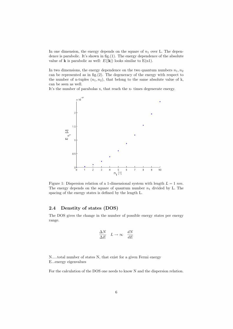
In one dimension, the energy depends on the square of n1 over L. The depen-dence is parabolic. It’s shown in fig.(1). The energy dependence of the absolutevalue of k is parabolic as well: E(|k|) looks similar to E(n1).
In two dimensions, the energy dependence on the two quantum numbers n1, n2
can be represented as in fig.(2). The degeneracy of the energy with respect tothe number of n-tuples (n1, n2), that belong to the same absolute value of k,can be seen as well.It’s the number of parabolas x, that reach the x- times degenerate energy.
Figure 1: Dispersion relation of a 1-dimensional system with length L = 1 nm.The energy depends on the square of quantum number n1 divided by L. Thespacing of the energy states is defined by the length L.
2.4 Denstity of states (DOS)
The DOS gives the change in the number of possible energy states per energyrange.
∆N∆E
L→∞ dN
dE
N.....total number of states N, that exist for a given Fermi energyE...energy eigenvalues
For the calculation of the DOS one needs to know N and the dispersion relation.
6
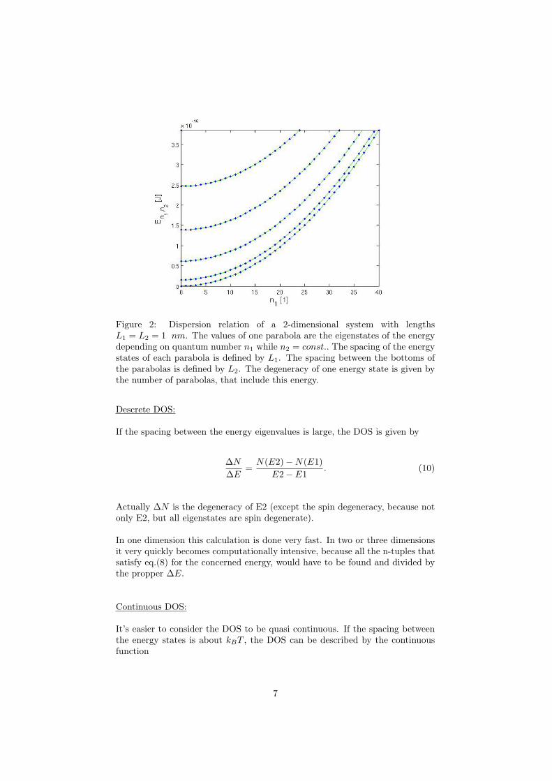
Figure 2: Dispersion relation of a 2-dimensional system with lengthsL1 = L2 = 1 nm. The values of one parabola are the eigenstates of the energydepending on quantum number n1 while n2 = const.. The spacing of the energystates of each parabola is defined by L1. The spacing between the bottoms ofthe parabolas is defined by L2. The degeneracy of one energy state is given bythe number of parabolas, that include this energy.
Descrete DOS:
If the spacing between the energy eigenvalues is large, the DOS is given by
∆N∆E
=N(E2)−N(E1)
E2− E1. (10)
Actually ∆N is the degeneracy of E2 (except the spin degeneracy, because notonly E2, but all eigenstates are spin degenerate).
In one dimension this calculation is done very fast. In two or three dimensionsit very quickly becomes computationally intensive, because all the n-tuples thatsatisfy eq.(8) for the concerned energy, would have to be found and divided bythe propper ∆E.
Continuous DOS:
It’s easier to consider the DOS to be quasi continuous. If the spacing betweenthe energy states is about kBT , the DOS can be described by the continuousfunction
7
dN
dE(11)
if the system is large in the dimension the electrons are considered to be quasifree.
In this case N can be calculated with the Fermi sphere.The Fermi sphere is a model for the Fermi surface (k-space), which fits well, ifthe period L (real space) becomes large.Large L causes small spacing of k. Hence the single state volumes are smallenough to be almost completely adjusted into the Fermi sphere.
2∑l
Θ(E − El) n=0
N(E) = 2∑l
Θ(E − El)VkΩk
+N∗ n=1,2
2VkΩk
+N∗ n=3
(12)
n......dimension of the systemΘ......................Heavyside stepfunctionk....wave vectorVk....Volume of the Fermi sphere (in k-space)Ωk....Volume, a single state takes in k-spaceN∗....extra states
The factor of two accounts for the spin degeneracy of a state.N∗ takes extra states in account.
Using the dispersion relation, the fermivector in the equation above can be ex-pressed in terms of energy.The DOS is given by the derivation of N(E) with respect to E.
Notice, that the calculation of N is valid for both specifications of k (eq.(6) and(7)), even though there’s a factor of two in k2 and k2 can be zero and negative.
k1 =n1 · πL1
n1 = 1, 2, 3...
k2 = ±n2 · 2πL2
n2 = 0, 1, 2, 3...
(13)
8

For a given Fermi energy E
E = ~2
2m ·n1·πL = ~2
2m ·n2·2πL
(14)
followsn2 =
n1
2
With eq.(12) follows
N1 = 2 ·n1
πLπL
= 2n1 = 4n2 = 2 ·n2
2πL
2πL
= N2
(15)
The two states at k = 0 for N2 are not necessary to mention, because they don’tinfluence the DOS, which is the derivation of N.
2.4.1 0-dimensional DOS
Since the energy levels of systems, that are quantized in all three dimensions are
discrete, the DOS is a couple of delta functions with peaks at discrete energies.
The height of the peak is the total number of degeneracies of the energy level.
The spin degeneracy causes a factor of two.
D0(E) = 2 · ni ·∑
l δ(E − El)
(16)
δ....Dirac delta functionEl....discrete energies En1,n2,n3
ni.....degeneracy of the energy El besides the spin degeneracy
Exemplary values for ni are listed in table (2.4.1).
2.4.2 1-dimensional DOS
If a quantum dot is enlarged in one dimension to the length L the system be-comes 1-dimensional.
9
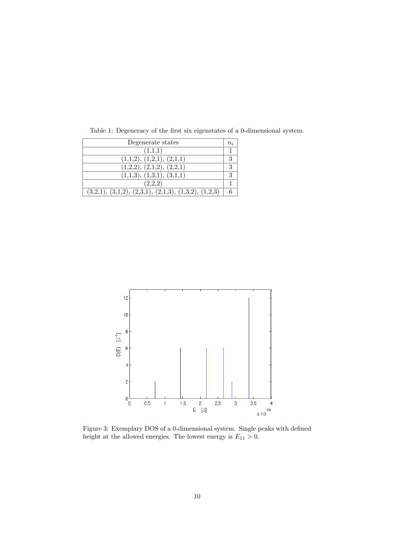
Table 1: Degeneracy of the first six eigenstates of a 0-dimensional system.
Degenerate states ni(1,1,1) 1
(1,1,2), (1,2,1), (2,1,1) 3(1,2,2), (2,1,2), (2,2,1) 3(1,1,3), (1,3,1), (3,1,1) 3
(2,2,2) 1(3,2,1), (3,1,2), (2,3,1), (2,1,3), (1,3,2), (1,2,3) 6
Figure 3: Exemplary DOS of a 0-dimensional system. Single peaks with definedheight at the allowed energies. The lowest energy is E11 > 0.
10
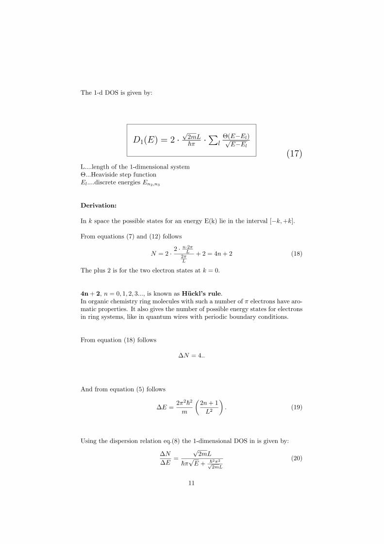
The 1-d DOS is given by:
D1(E) = 2 ·√
2mL~π ·
∑l
Θ(E−El)√E−El
(17)
L....length of the 1-dimensional systemΘ...Heaviside step functionEl....discrete energies En2,n3
Derivation:
In k space the possible states for an energy E(k) lie in the interval [−k,+k].
From equations (7) and (12) follows
N = 2 ·2 · n·2πL
2πL
+ 2 = 4n+ 2 (18)
The plus 2 is for the two electron states at k = 0.
4n + 2, n = 0, 1, 2, 3..., is known as Huckl’s rule.In organic chemistry ring molecules with such a number of π electrons have aro-matic properties. It also gives the number of possible energy states for electronsin ring systems, like in quantum wires with periodic boundary conditions.
From equation (18) follows
∆N = 4..
And from equation (5) follows
∆E =2π2~2
m
(2n+ 1L2
). (19)
Using the dispersion relation eq.(8) the 1-dimensional DOS in is given by:
∆N∆E
=√
2mL~π√E + ~2π2√
2mL
(20)
11
If L becomes larger and the electrons are regarded as quasi free, the limit L −→∞ can be taken and eq.(20) becomes
D1(E) =√
2mL~π√E. (21)
which is the derivation of
N = 4n+ 2 (∗)=
√8mLh
·√E + 2 = N(E) (22)
(*)...using the dispersion relation eq.(8)
with respect to E.
If more than the first energy state is used, eq. (21) becomes eq.(17).
Equation (17) can be regarded as a discrete 2-dimensional DOS (transition toa 2-dimensional system).
The factor of two in the front accounts for the two extra degeneracies causedby the second quantum number n2, the energy is now depending on.(The dependence of the third quantum number exists, but there will be consid-ered the transition to two dimensions first, which means that the energy mainlychanges with n1 and n2.)
From the considerations above we know, that enlarging the energy from Ento En+1 causes four more states, the spin degeneracy included.
When making the transition from one to two dimensions there’s no further spindegeneracy but only degeneracy caused by another quantum number, which isa factor of two.
Building the sum is only possible, because the summands are continuous func-tions of E.It’s not possible to do the same with discrete summands (eq.(20)).
∆N3
∆E36= ∆N1
∆E1+
∆N2
∆E2(23)
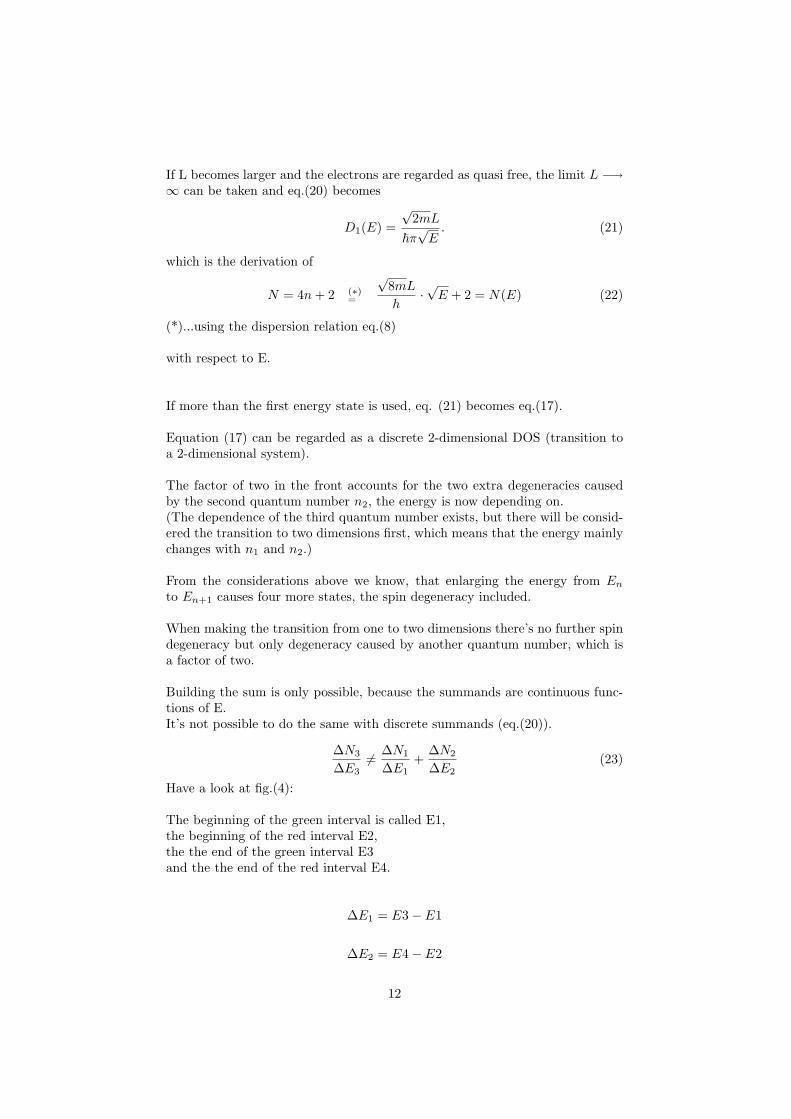
Have a look at fig.(4):
The beginning of the green interval is called E1,the beginning of the red interval E2,the the end of the green interval E3and the the end of the red interval E4.
∆E1 = E3− E1
∆E2 = E4− E2
12
∆E3 = E3− E2
∆E3 is the difference between energies of two different 1-dimensional densitiesand the proper ∆N is not ∆N1 + ∆N2.
Figure 4: A couple of overlapping 1-dimensional densities of states.
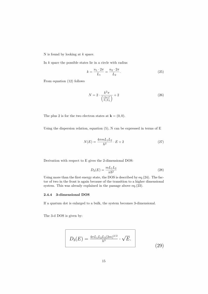
2.4.3 2-dimensional DOS
If a quatum dot is enlarged to a plane, the system becomes 2-dimensional.
The 2-d DOS is given by:
D2(E) = 2 · mL1L2
~2π ·∑
l Θ(E − El)
(24)
L1, L2....size of the 2-dimensional systemΘ...Heaviside step functionEl....discrete energies En3
Derivation:
If the spacing of the energy eigenvalues is smaller than kBT the van Hovensingularities of the 1-dimensional DOS are that close together, that they are nolonger distinguishable.
13
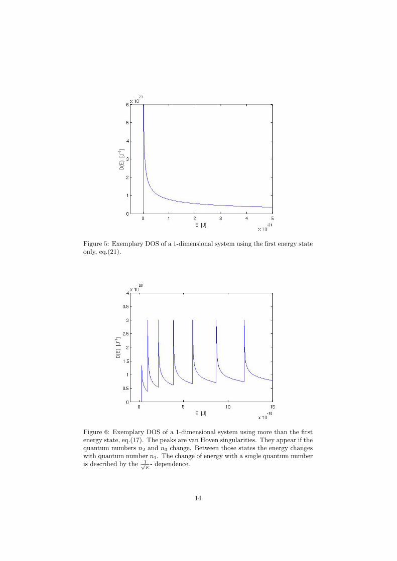
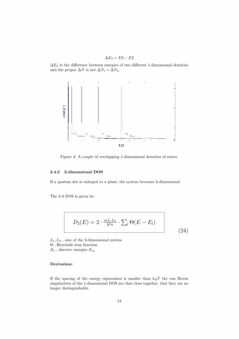
Figure 5: Exemplary DOS of a 1-dimensional system using the first energy stateonly, eq.(21).
Figure 6: Exemplary DOS of a 1-dimensional system using more than the firstenergy state, eq.(17). The peaks are van Hoven singularities. They appear if thequantum numbers n2 and n3 change. Between those states the energy changeswith quantum number n1. The change of energy with a single quantum numberis described by the 1√
E- dependence.
14
N is found by looking at k space.
In k space the possible states lie in a circle with radius
k =n1 · 2πL1
=n2 · 2πL2
. (25)
From equation (12) follows
N = 2 · k2π((2π)2
L1L2
) + 2 (26)
The plus 2 is for the two electron states at k = (0, 0).
Using the dispersion relation, equation (5), N can be expressed in terms of E
N(E) =4πmL1L2
h2· E + 2 (27)
Derivation with respect to E gives the 2-dimensional DOS:
D2(E) =mL1L2
π~2(28)
Using more than the first energy state, the DOS is described by eq.(24). The fac-tor of two in the front is again because of the transition to a higher dimensionalsystem. This was already explained in the passage above eq.(23).
2.4.4 3-dimensional DOS
If a quatum dot is enlarged to a bulk, the system becomes 3-dimensional.
The 3-d DOS is given by:
D3(E) = 4πL1L2L3(2m)3/2
h3 ·√E.
(29)
15
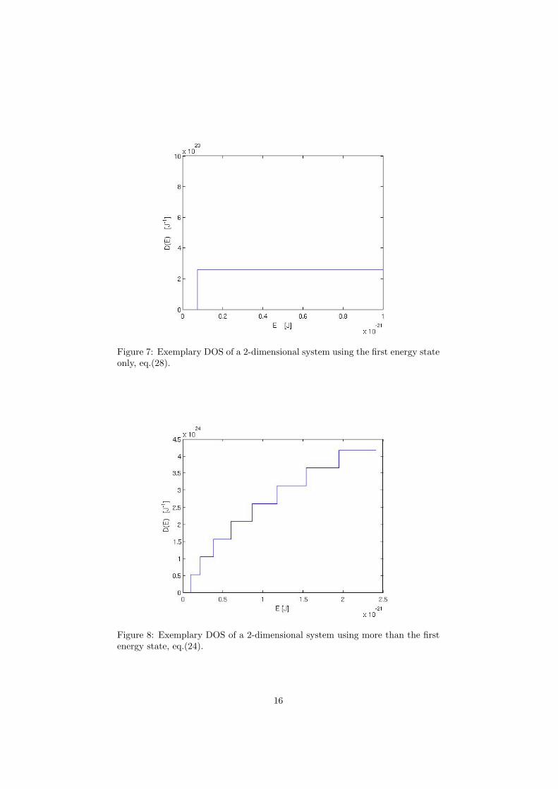
Figure 7: Exemplary DOS of a 2-dimensional system using the first energy stateonly, eq.(28).
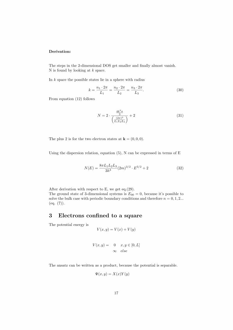
Figure 8: Exemplary DOS of a 2-dimensional system using more than the firstenergy state, eq.(24).
16
Derivation:
The steps in the 2-dimensional DOS get smaller and finally almost vanish.N is found by looking at k space.
In k space the possible states lie in a sphere with radius
k =n1 · 2πL1
=n2 · 2πL2
=n3 · 2πL3
. (30)
From equation (12) follows
N = 2 ·4k3π
3((2π)3
L1L2L3
) + 2 (31)
The plus 2 is for the two electron states at k = (0, 0, 0).
Using the dispersion relation, equation (5), N can be expressed in terms of E
N(E) =8πL1L2L3
3h3(2m)3/2 · E3/2 + 2 (32)
After derivation with respect to E, we get eq.(29).The ground state of 3-dimensional systems is E00 = 0, because it’s possible tosolve the bulk case with periodic boundary conditions and therefore n = 0, 1, 2...(eq. (7)).
3 Electrons confined to a square
The potential energy isV (x, y) = V (x) + V (y)
V (x, y) = 0 x, y ∈ [0, L]∞ else
The ansatz can be written as a product, because the potential is separable.
Ψ(x, y) = X(x)Y (y)
17
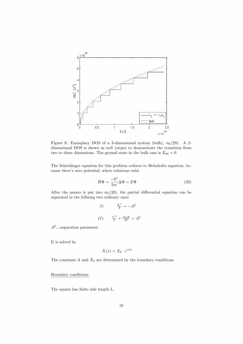
Figure 9: Exemplary DOS of a 3-dimensional system (bulk), eq.(29). A 2-dimensional DOS is shown as well (steps) to demonstrate the transition fromtwo to three dimensions. The ground state in the bulk case is E00 = 0.
The Schrodinger equation for this problem reduces to Helmholtz equation, be-cause there’s zero potential, where solutions exist.
HΨ =−~2
2m∆Ψ = EΨ (33)
After the ansatz is put into eq.(33), the partial differential equation can beseparated in the follwing two ordinary ones:
I) X′′
X = −A2
II) Y ′′
Y + 2mE~2 = A2
A2....separation parameter
I) is solved by
X(x) = X0 · eiAx
The constants A and X0 are determined by the boundary conditions.
Boundary conditions:
The square has finite side length L.
18
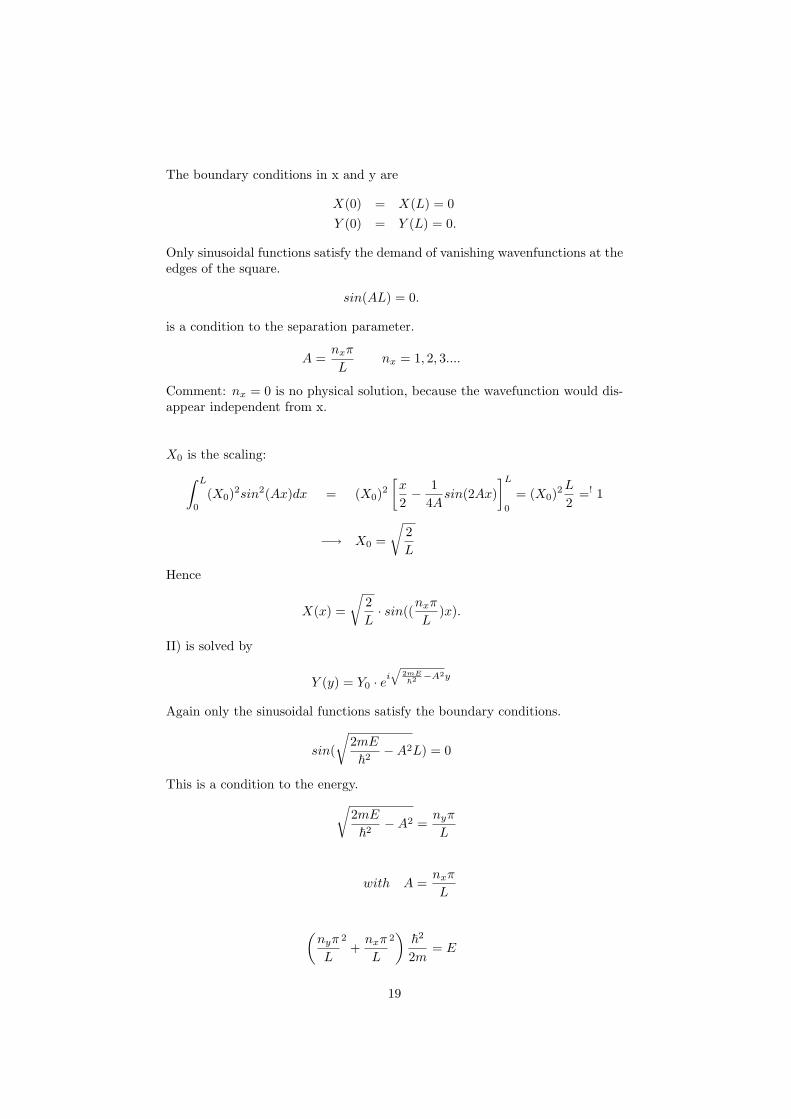
The boundary conditions in x and y are
X(0) = X(L) = 0Y (0) = Y (L) = 0.
Only sinusoidal functions satisfy the demand of vanishing wavenfunctions at theedges of the square.
sin(AL) = 0.
is a condition to the separation parameter.
A =nxπ
Lnx = 1, 2, 3....
Comment: nx = 0 is no physical solution, because the wavefunction would dis-appear independent from x.
X0 is the scaling:∫ L
0
(X0)2sin2(Ax)dx = (X0)2
[x
2− 1
4Asin(2Ax)
]L0
= (X0)2L
2=! 1
−→ X0 =
√2L
Hence
X(x) =
√2L· sin((
nxπ
L)x).
II) is solved by
Y (y) = Y0 · eiq
2mE~2 −A2y
Again only the sinusoidal functions satisfy the boundary conditions.
sin(
√2mE~2−A2L) = 0
This is a condition to the energy.√2mE~2−A2 =
nyπ
L
with A =nxπ
L
(nyπ
L
2+nxπ
L
2)
~2
2m= E
19
Hence
Y (y) = Y0 · sin((nyπ
L)y).
Y0 is found by calculating the scale.∫ L
0
(Y0)2sin2(nyπ
Ly)dx = (Y0)2
[y
2− 1
4(nyπL )
sin(2(nyπ
L)y)]L
0
= (Y0)2L
2= 1
−→ Y0 =
√2L
Finally the eigenfunctions and eigenvalues for electrons in a square of finite sizeL are:
Ψ(x, y) =2L· sin(
nxπ · xL
) · sin(nyπ · yL
)
(34)
E =~2
2m·(
(nyπ
L)2 + (
nxπ
L)2)
(35)
nx, ny = 1, 2, 3....
3.1 Dispersion relation
E = ~2
2m ·((nyπL )2 + (nxπL )2
)(36)
nx, ny = 1, 2, 3....
The energy depends on the two quantum numbers nx and ny and the length ofthe square L.
3.2 Density of states
The length L of the square characterizes the DOS.
If L is very small, the energy states are widely spaced (∆E > kBT ). The DOSis described by the delta peaks of the 0-dimensional system.Have a look at chapter (2.4.1) and figure (11).
If L becomes that large, that the spacing of the delta functions is about kBT andthe DOS can be described by the quasicontinuous 2-dimensional DOS, which isa constant (using the first energy state only).
20
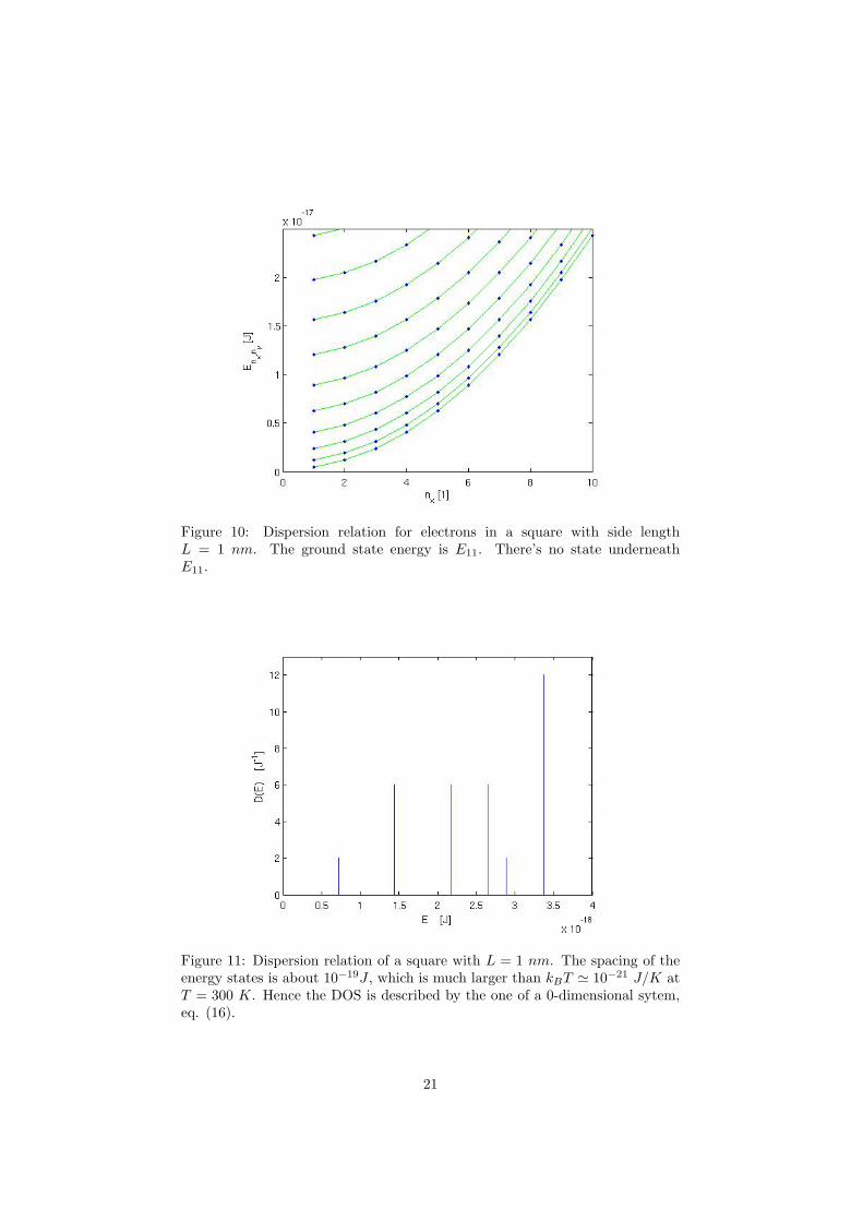
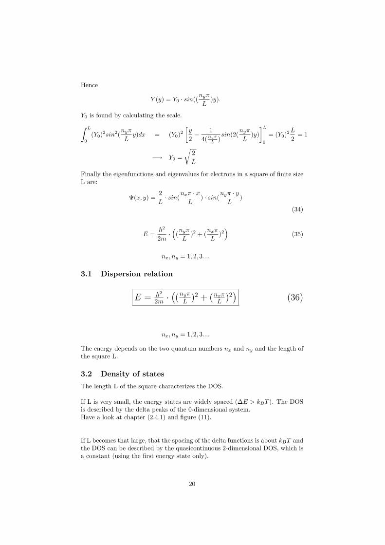
Figure 10: Dispersion relation for electrons in a square with side lengthL = 1 nm. The ground state energy is E11. There’s no state underneathE11.
Figure 11: Dispersion relation of a square with L = 1 nm. The spacing of theenergy states is about 10−19J , which is much larger than kBT ' 10−21 J/K atT = 300 K. Hence the DOS is described by the one of a 0-dimensional sytem,eq. (16).
21
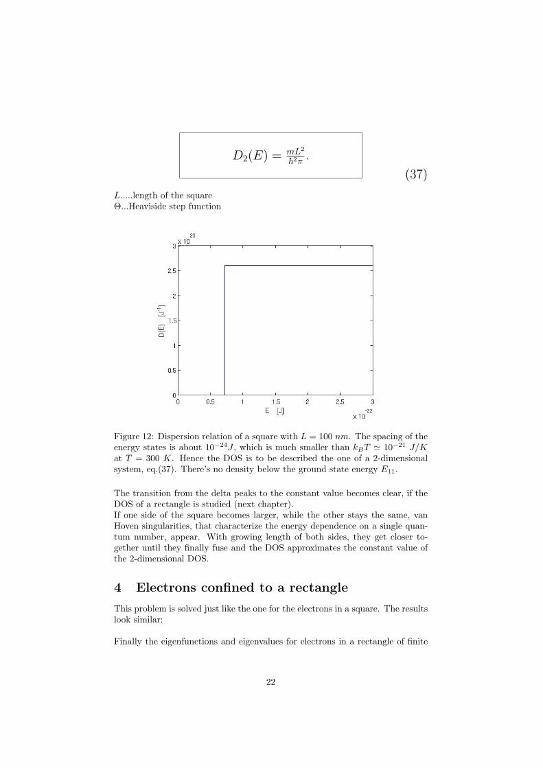
D2(E) = mL2
~2π .
(37)
L.....length of the squareΘ...Heaviside step function
Figure 12: Dispersion relation of a square with L = 100 nm. The spacing of theenergy states is about 10−24J , which is much smaller than kBT ' 10−21 J/Kat T = 300 K. Hence the DOS is to be described the one of a 2-dimensionalsystem, eq.(37). There’s no density below the ground state energy E11.
The transition from the delta peaks to the constant value becomes clear, if theDOS of a rectangle is studied (next chapter).If one side of the square becomes larger, while the other stays the same, vanHoven singularities, that characterize the energy dependence on a single quan-tum number, appear. With growing length of both sides, they get closer to-gether until they finally fuse and the DOS approximates the constant value ofthe 2-dimensional DOS.
4 Electrons confined to a rectangle
This problem is solved just like the one for the electrons in a square. The resultslook similar:
Finally the eigenfunctions and eigenvalues for electrons in a rectangle of finite
22
size L are:
Ψ(x, y) =2√LxLy
· sin(nxπ · xLx
) · sin(nyπ · yLy
)
(38)
E =~2
2m·(
(nyπ
Ly)2 + (
nxπ
Lx)2
)(39)
nx, ny = 1, 2, 3....
4.1 Dispersion relation
E = ~2
2m ·(
(nyπLy
)2 + (nxπLx )2)
(40)
nx, ny = 1, 2, 3....
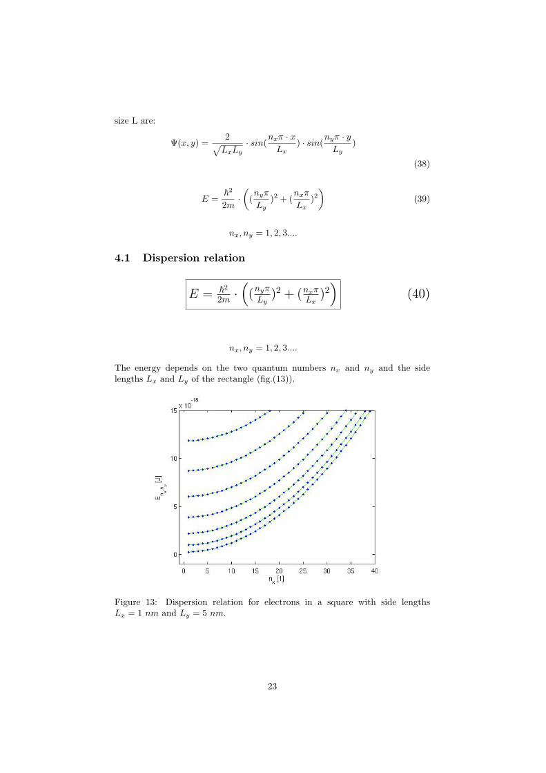
The energy depends on the two quantum numbers nx and ny and the sidelengths Lx and Ly of the rectangle (fig.(13)).
Figure 13: Dispersion relation for electrons in a square with side lengthsLx = 1 nm and Ly = 5 nm.
23
4.2 Density of states
The lengths of the sides of the rectangle characterize the DOS.
If both sides are very small, the energy states are widely spaced. The DOS is acombination of the 1-dimensional densities in nx and ny and shows van Hovensingularities.
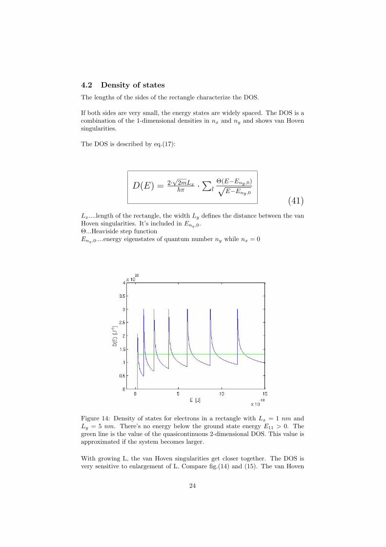
The DOS is described by eq.(17):
D(E) = 2·√
2mLx~π ·
∑l
Θ(E−Eny,0)√E−Eny,0
(41)
Lx....length of the rectangle, the width Ly defines the distance between the vanHoven singularities. It’s included in Eny,0.Θ...Heaviside step functionEny,0....energy eigenstates of quantum number ny while nx = 0
Figure 14: Density of states for electrons in a rectangle with Lx = 1 nm andLy = 5 nm. There’s no energy below the ground state energy E11 > 0. Thegreen line is the value of the quasicontinuous 2-dimensional DOS. This value isapproximated if the system becomes larger.
With growing L, the van Hoven singularities get closer together. The DOS isvery sensitive to enlargement of L. Compare fig.(14) and (15). The van Hoven
24
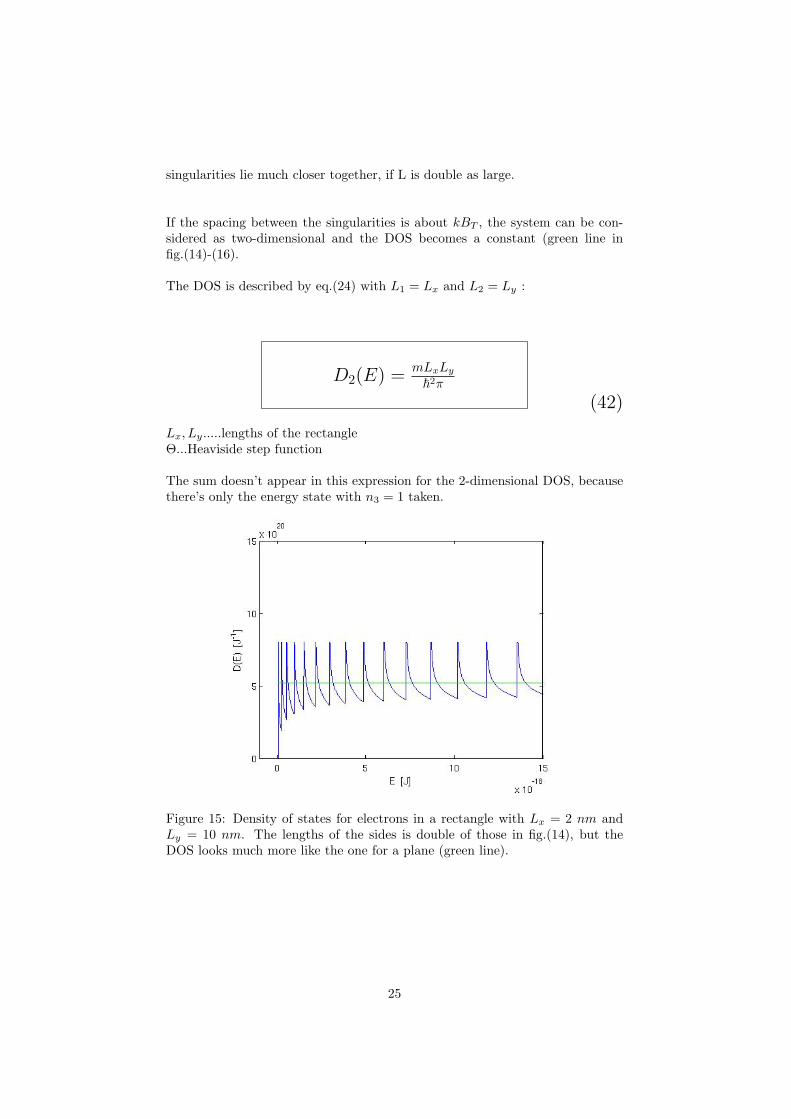
singularities lie much closer together, if L is double as large.
If the spacing between the singularities is about kBT , the system can be con-sidered as two-dimensional and the DOS becomes a constant (green line infig.(14)-(16).
The DOS is described by eq.(24) with L1 = Lx and L2 = Ly :
D2(E) =mLxLy
~2π
(42)
Lx, Ly.....lengths of the rectangleΘ...Heaviside step function
The sum doesn’t appear in this expression for the 2-dimensional DOS, becausethere’s only the energy state with n3 = 1 taken.
Figure 15: Density of states for electrons in a rectangle with Lx = 2 nm andLy = 10 nm. The lengths of the sides is double of those in fig.(14), but theDOS looks much more like the one for a plane (green line).
25
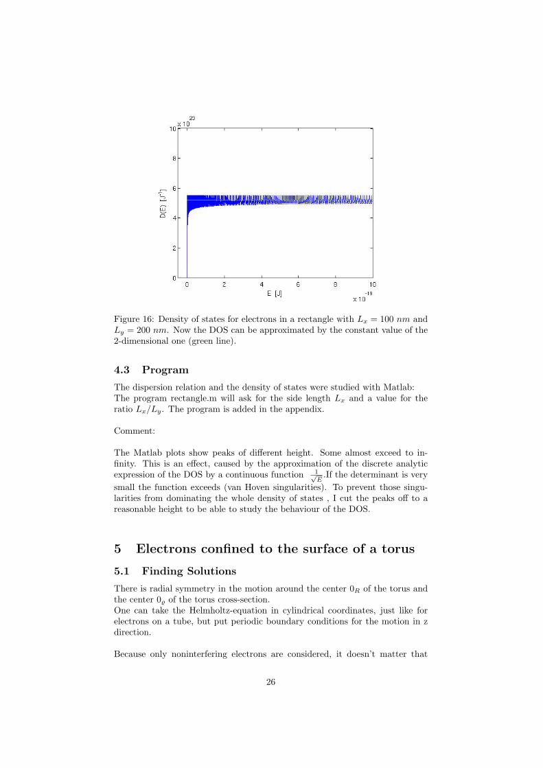
Figure 16: Density of states for electrons in a rectangle with Lx = 100 nm andLy = 200 nm. Now the DOS can be approximated by the constant value of the2-dimensional one (green line).
4.3 Program
The dispersion relation and the density of states were studied with Matlab:The program rectangle.m will ask for the side length Lx and a value for theratio Lx/Ly. The program is added in the appendix.
Comment:
The Matlab plots show peaks of different height. Some almost exceed to in-finity. This is an effect, caused by the approximation of the discrete analyticexpression of the DOS by a continuous function 1√
E.If the determinant is very
small the function exceeds (van Hoven singularities). To prevent those singu-larities from dominating the whole density of states , I cut the peaks off to areasonable height to be able to study the behaviour of the DOS.
5 Electrons confined to the surface of a torus
5.1 Finding Solutions
There is radial symmetry in the motion around the center 0R of the torus andthe center 0% of the torus cross-section.One can take the Helmholtz-equation in cylindrical coordinates, just like forelectrons on a tube, but put periodic boundary conditions for the motion in zdirection.
Because only noninterfering electrons are considered, it doesn’t matter that
26
the inner circumference of the torus is smaller than the outer one. It’s possibleto transform the tube into a torus by calling the tube’s length L the circumfer-ence through the center of the torus.
This ansatz will be discussed underneath. It is also possible to make a sec-ond transformation (rolling out the tube) and treat the electrons in thetorus like electrons in a rectangle, using periodic boundary condi-tions (nx,ny = 0,1,2,3...).
Tube with periodic boundary conditions (alternative discussion):
L = 2Rπ (43)
In the chosen coordinate system r,ϕ and z are independent from each other andthe Hamilton Operator is separable. Therefore the solution can be written as aproduct of functions in the three cylindrical coordinates r, ϕ and z:
ψ(r, ϕ, z) = R(r)Φ(ϕ)Z(z) (44)
For a certain diameter % the R(r) becomes a Dirac-Delta and the ansatz reducesto
ψ(r, ϕ, z) = Φ(ϕ)Z(z) · c · δ(r − %) (45)
where c is the scaling-factor.
The Nabla operator in the Helmholtz-equation has to be transformed to cylin-drical coordinates (eq.(96)). The Nabla operating on R(r) is zero.
∆r =δ2
δr2+
1r
δ
δr
R(r) = c · δ(r − %)
The derivation of the delta distribution is by definition deligated to the deriva-tion of the function f(r), which is described by the distribution.
δ(f) =∫ ∞
0
δ(r − %)f(r)dr = f(%) = 1
δ′(f) = −δ(f ′) = −f ′(%) = 0
27
In this case the f(r) = 1 = f(%). Therefore the derivation of f(%) is zero andthe whole radial part of the Nabla operating on the wavefunction cancels out.
This fact was to be expected. Electrons on the surface of a torus move in threedimensions, but define an only 2-dimensional mathematical problem. This is,because the electrons on the surface of the torus, which is defined by the twofixed radii R and %, have only two degrees of freedom. One in ϕ and one in z.Therefore it’s sufficient to consider a problem in two dimensions with the ansatz
ψ = Φ(ϕ) · Z(z). (46)
The constant of the separation is chosen to be −m2. The two differential equa-tions are then
I) Φ′′
Φ = −m2
II) Z′′
Z = m2
%2 −2mEh2
(47)
The right side of equation II) is constant as well and will be called −k2.
Ad I): Equation (47,I) is solved by a solution of the following kind:
Φ(ϕ) = Aeimϕ +Be−imϕ (48)
There are two conditions that have to be satisfied by this solution:
• 1) Uniqueness on the surface, concerning the motion in phi
• 2) The probability to find the electron at any angular φ has to be one,which is a standardisation condition to the solution.
Those conditions determine the paramaters m and Φ0.
1) can be expressed as
Φ(ϕ) = Φ(ϕ+ 2π) (49)
28
meaning
Aeimϕ +Be−imϕ = Aeim(ϕ+2π) +Be−im(ϕ+2π)
= Aeimϕeim2π +Be−imϕe−im2π
It is only true, if
eim2π = e−im2π = 1
which can be achieved by m ∈ N0.
A more compact and common way to write the ansatz equation (48) is the fol-lowing, in which m ∈ Z.
Φ(ϕ) = Φ0eimϕ (50)
The factor Φ0 is determined by the second condition, the scaling.
∫ 2π
0
|Φ(ϕ)|2dϕ =∫ 2π
0
Φ · Φ∗dϕ = 1∫ 2π
0
Φ20eimϕe−imϕdϕ = Φ2
0 · ϕ|2π0 = Φ20 · 2π = 1
Φ0 =1√2π
The solutions in ϕ then are
Φ(ϕ) =1√2πeimϕ ,m ∈ Z (51)
Ad II): Equation (47,II) can be solved with a similar ansatz like the one forΦ(ϕ). Compare it with equation (50).
Z(z) = Aeikz (52)
29
A....constant real coefficient
k =
√2mEh2− m2
r2(53)
For the solution in Z there are two similar conditions as there are for the φ part:
• 1) Uniqueness concerning the motion in z direction (around the origin)
• 2) The probability to find the electron anywhere between z = 0 and z =2Rπ has to be 1, which is a standardization condition to the solution inZ.
In analogy to m, k has to be chosen properly, so that Z(z) is periodic in L andthus unique concerning the motion around the center of the torus.
Z(z) = Z(z + L)Aeikz = Aeik(z+L) = AeikzAeikL
eikL = 1
This is satisfied if
k = n · 2πL
n ∈ Z (54)
A is the scaling factor. Since the wavefunction disappears for z ∈ (−∞, 0) andz ∈ (L,∞), the limits of the scaling integral can be set from 0 to L.
∫ L
0
|Z(z)|2dz =∫ L
0
A2eikze−ikzdz
A2 · L = 1
A =1√L
Finally the radial part is scaled too:
∫ ∞0
c2δ2(r − %)rdr =∫ ∞
0
c2δ(r − %)%dr = c2% =! 1
c =1√%
(55)
30
The solution ψ is then
ψ(ϕ, z) = 1√2π·L
1√% · e
imϕ · eikz · δ(r − %)
k = n · 2πL
L = 2Rπ n,m ∈ Z (56)
5.2 Dispersion relation
The energy is the expectation value of the Hamilton operator:
E = 〈ψ|H|ψ〉 (57)
For the solution eq.(56) a tube was taken and periodic boundary conditions putin.
If the torus was treated as a rectangle with periodic boundary conditions, thetwo degrees of freedom would be x and z.And the wavefunction:
ψ2(x, z) = 1√LxLz
eikxxeikzz
kx = nx2πLx
kz = nz2πLz
nx, nz ∈ Z
Lx=2%π Lz=2Rπ (58)
The solutions can also be found, if the ansatz is a product of two independentmovements in the angulars ϑ and ϕ. (Actually the momenta aren’t linear, buttorsional.)
ψ3(ϕ, θ) = C · eimϕ · einθ · δ(r − %) n,m ∈ Z(59)
For calculating the dispersion relation it’s equal to use eq.(56), (58) or (59).
31
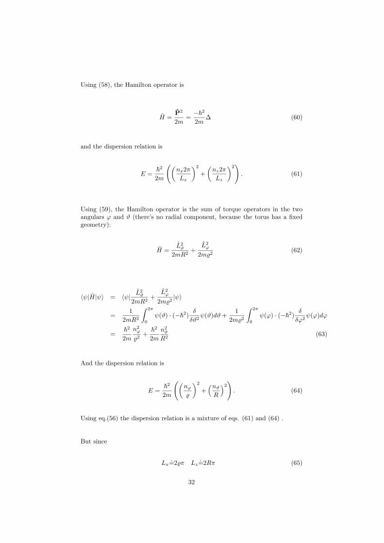
Using (58), the Hamilton operator is
H =P2
2m=−~2
2m∆ (60)
and the dispersion relation is
E =~2
2m
((nx2πLx
)2
+(nz2πLz
)2). (61)
Using (59), the Hamilton operator is the sum of torque operators in the twoangulars ϕ and ϑ (there’s no radial component, because the torus has a fixedgeometry):
H =L2ϑ
2mR2+
L2ϕ
2m%2(62)
〈ψ|H|ψ〉 = 〈ψ| L2ϑ
2mR2+
L2ϕ
2m%2|ψ〉
=1
2mR2
∫ 2π
0
ψ(ϑ) · (−~2)δ
δϑ2ψ(ϑ)dϑ+
12m%2
∫ 2π
0
ψ(ϕ) · (−~2)δ
δϕ2ψ(ϕ)dϕ
=~2
2mn2ϕ
%2+
~2
2mn2ϑ
R2(63)
And the dispersion relation is
E =~2
2m
((nϕ%
)2
+(nϑR
)2). (64)
Using eq.(56) the dispersion relation is a mixture of eqs. (61) and (64) .
But since
Lx=2%π Lz=2Rπ (65)
32
the solutions ψ, ψ2 and ψ3 as well as the dispersion relations E(nx, nz) andE(nϕ, nϑ) are equal.
Because the significant parameters ϕ and R are used, eq.(64) is called the
DISP of a torus
E = ~2
2m
((nϕ%
)2+(nϑR
)2).
(66)
nϑ, nϕ = 0, 1, 2, 3.... (67)
Because of the discussion above it’s clear, that the DISP and DOS of a torusare very similar to the one of the rectangle. The only differences are
L = 2Rπ (68)
andn = 0→ E0 = 0. (69)
5.3 Density of states
The electrons on the surface of a torus is a two dimensional problem.The energy depends on the two quantum numbers nϕ and nϑ and on the tworadii R and %.
The total number of states N in calculated using eq.(12) and k from the disper-sion relation eq.(66).
∆kϕ =1%
and ∆kR =1R. (70)
N = 2 · k2 · π(1%·R
) + 2. (71)
33
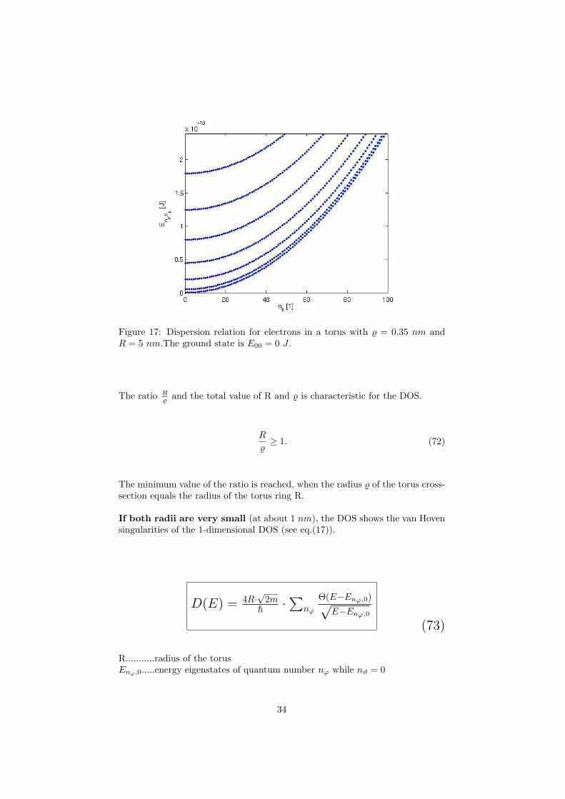
Figure 17: Dispersion relation for electrons in a torus with % = 0.35 nm andR = 5 nm.The ground state is E00 = 0 J .
The ratio R% and the total value of R and % is characteristic for the DOS.
R
%≥ 1. (72)
The minimum value of the ratio is reached, when the radius % of the torus cross-section equals the radius of the torus ring R.
If both radii are very small (at about 1 nm), the DOS shows the van Hovensingularities of the 1-dimensional DOS (see eq.(17)).
D(E) = 4R·√
2m~ ·
∑nϕ
Θ(E−Enϕ,0)√E−Enϕ,0
(73)
R...........radius of the torusEnϕ,0.....energy eigenstates of quantum number nϕ while nϑ = 0
34
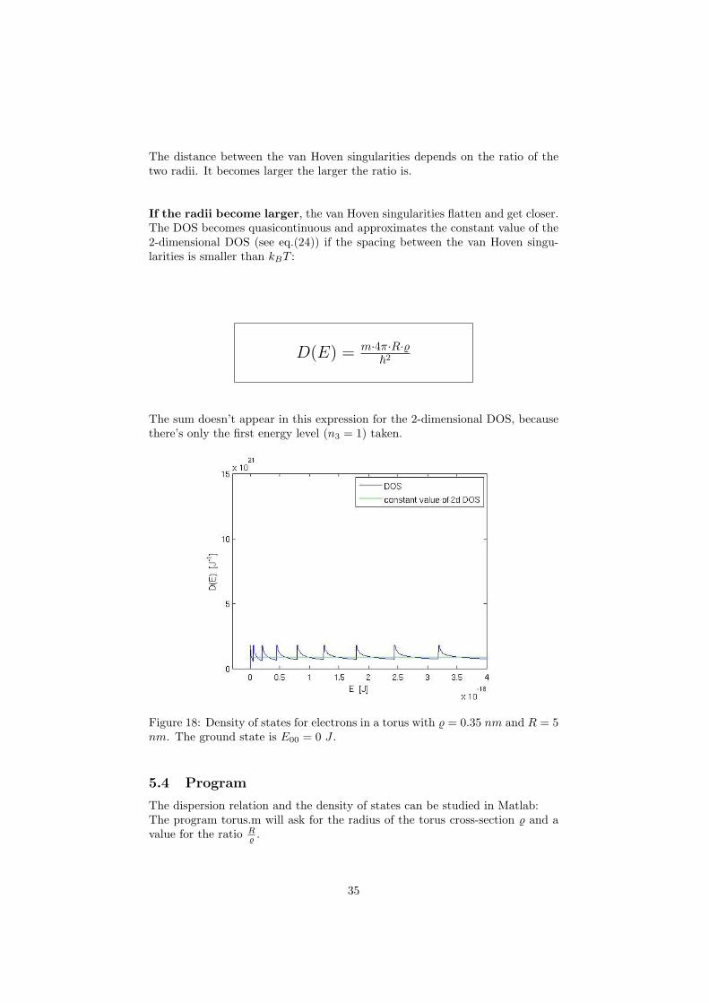
The distance between the van Hoven singularities depends on the ratio of thetwo radii. It becomes larger the larger the ratio is.
If the radii become larger, the van Hoven singularities flatten and get closer.The DOS becomes quasicontinuous and approximates the constant value of the2-dimensional DOS (see eq.(24)) if the spacing between the van Hoven singu-larities is smaller than kBT :
D(E) = m·4π·R·%~2
The sum doesn’t appear in this expression for the 2-dimensional DOS, becausethere’s only the first energy level (n3 = 1) taken.
Figure 18: Density of states for electrons in a torus with % = 0.35 nm and R = 5nm. The ground state is E00 = 0 J .
5.4 Program
The dispersion relation and the density of states can be studied in Matlab:The program torus.m will ask for the radius of the torus cross-section % and avalue for the ratio R
% .
35
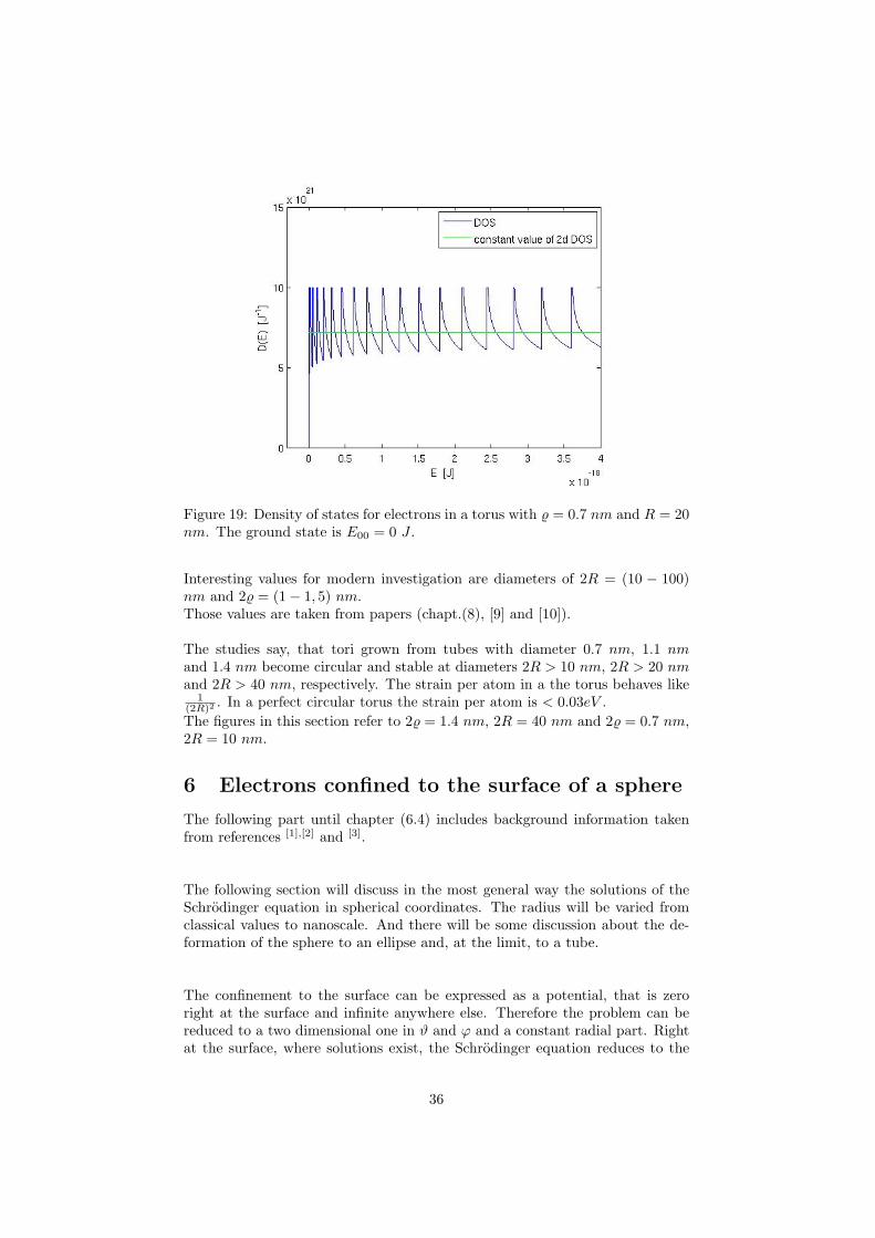
Figure 19: Density of states for electrons in a torus with % = 0.7 nm and R = 20nm. The ground state is E00 = 0 J .
Interesting values for modern investigation are diameters of 2R = (10 − 100)nm and 2% = (1− 1, 5) nm.Those values are taken from papers (chapt.(8), [9] and [10]).
The studies say, that tori grown from tubes with diameter 0.7 nm, 1.1 nmand 1.4 nm become circular and stable at diameters 2R > 10 nm, 2R > 20 nmand 2R > 40 nm, respectively. The strain per atom in a the torus behaves like
1(2R)2 . In a perfect circular torus the strain per atom is < 0.03eV .The figures in this section refer to 2% = 1.4 nm, 2R = 40 nm and 2% = 0.7 nm,2R = 10 nm.
6 Electrons confined to the surface of a sphere
The following part until chapter (6.4) includes background information takenfrom references [1],[2] and [3].
The following section will discuss in the most general way the solutions of theSchrodinger equation in spherical coordinates. The radius will be varied fromclassical values to nanoscale. And there will be some discussion about the de-formation of the sphere to an ellipse and, at the limit, to a tube.
The confinement to the surface can be expressed as a potential, that is zeroright at the surface and infinite anywhere else. Therefore the problem can bereduced to a two dimensional one in ϑ and ϕ and a constant radial part. Rightat the surface, where solutions exist, the Schrodinger equation reduces to the
36
Helmholtz-equation (eq.(1)) with the Nabla of eq.(97).
Since the spherical coordinates are independent for this problem, the ansatz canbe written as a product with a delta function for the radial part:
ψ(r, ϕ, ϑ) = Φ(ϕ) ·Θ(ϑ) · c · δ(r − %). (74)
The Schrodinger equation for this problem is the Helmholtz equation, becausewe concentrate on the surface, where the potential is zero.
HΨ(r, ϕ, ϑ) =p2
2mΨ(r, ϕ, ϑ) =
−~2
2m∆ϑϕ = E ·Ψ(r, ϕ, ϑ) (75)
∆ϑϕ is the angular part of the Nabla operator.There’s no radial part, because r = const..The Nabla operator doesn’t affect the radial part of the ansatz.
The differential equation that has to be solved for that problem is:
−~2
2m ∆ϑϕ = E ·Ψ(r, ϕ, ϑ)
−~2
2m ·1r2 ·
[1
sin(ϑ)· δδϑ
(sin(ϑ) · ΦΘ′) +1
sin2(ϑ)· Φ′′Θ
]= E ·Ψ (76)
6.1 Background for radial symmetric problems
In radial symmetric potentials, it’s often useful to transform the Cartesian co-ordinates to spherical ones. The Nabla operator has to be transformed too.In the following section it will be shown, that the angular part of the Nabla isclosely connected to the square of the operator of the angular momentum L.And further that the radial symmetric problem is solved, if the eigenvalues forL and L2 are found.
[L2, Li] = [P2, Li] = [r2, Li] = 0 (77)
Since L2 as well as P2 and r2 commute with one component of the operator ofangular momentum, they are all invariant with respect to rotation.Thus in radial symmetric problems, where V (r) = V (r), the whole Hamiltonianis invariant with respect to rotation.This means that H, L2, P2, r2 and Li have a common set of eigenfunctions.
The eigenvalue problem for L2 and Li can be analytically solved and the eigen-values of the Hamiltonian for the electrons on the surface of a sphere are theeigenvalues of L2 times a constant, because
−~2
2m∆ϑ,ϕ =
L2
2mr2, r = const. (78)
37
as we will see.
The following section will concentrate on the eigenvalue problem of L2.The way of solving the eigenvalue problem will be sketched. In the end thesolutions for the angular part of a radial symmetric problem will be presented.
6.2 Operators of angular momentum:
Each operator that has hermetian (see chapter 7) components Ji and satisfies
[Ji, Jj ] = i~∑k
εijkJk ,∀i, j (79)
describes an operator of angular momentum.
If two operators don’t commute, e.g.
L1L2 − L2L1 = i~L3, (80)
their expectation values can’t be measured sharply at the same time. Theyoscillate around the x3 axis. The factor i~ has is origin in the uncertaintyrelation
[xi, pj ] = i~δij . (81)
If two operators commute,
[J2, Ji] = 0 (82)
they build a system of observables, that can be measured sharply at the sametime. Without restriction Ji is chosen to be Jz.
J2 and Jz satisfy the following eigenvalue equations:
J2|αjm > = ~2αj |αjm >
Jz|αjm > = ~m|αjm > (83)
~ was pulled out of the eigenvalues, so that αj and m are dimensionless values.This is, because the expectation value of a linear momentum operator can beexpressed in multiples of ~. Since J2 and Jz are hermetian (see chapter ??) theeigenfunctions build a basis and the eigenvalues are real.
The solution is found by introducing step operators J± = Lx ± iLy that worksimilar like a+ and a for the harmonic oscillator. it can be shown, that J±working on the eigenfunctions, the eigenvalues for J2 stay the same and theeigenvalues of Jz raise or fall about 1.
J2(J±|αjm >) = ~2αj(J±|αjm >)Jz(J±|αjm >) = ~(m±1)(J±|αjm >) (84)
38
Properties of the eigenvalues:
• −√αj ≤m ≤ √αj
Since Ji is hermetian, the expectation values of J2x and J2
y are never nega-tive. Consequently J2−J2
z = J2x +J2
y has also a not negative expectation-value in any state. For |αjm > the expectation value was ~2(αj−m2) ≥ 0,which verifies the first property.
• There’s a maximum and a minimum for m and they are unique.
Existence:
αj stays the same when J± is applied on |αjm > and encloses m, whichrises or lowers with the number n of applications
Jz(Jn±|αjm >) = ~(m± n)(Jn±|αjm >).
Uniqueness:Application of Jn− decreases the maximum of m to the minimum in n steps.Therefore
mmax −mmin = n, n ∈ N.
• αj is definded by mmax and mmax also defines mmin.
Application of J−J+ on |αjmmax > gives an expression for αj :
αj = mmax(mmax + 1) = j(j + 1)
Application of J+J− on |αjmmin > leads to an expression for mmin:
j(j + 1) = mmin(mmin − 1)
Solutions are mmin = j + 1 and mmin = −j. The first one drops out,because j is already the maximum.
• j are half integers, because of the results above: j − mmin = n andmmin = −j.
Summarized results:
• Eigenvalues of J2: ~2j(j + 1), j = 0, 12 , 1,
32 , 2....
• Eigenvalues of Jz are ~m, m = −j,−j + 1, ......, j − 1, j
• lets call the eigenstates |αjm >= |jm >
39
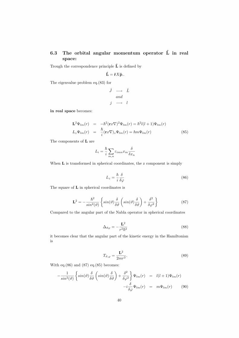
6.3 The orbital angular momentum operator L in realspace:
Trough the correspondence principle L is defined by
L = rXp..
The eigenvalue problem eq.(83) for
J −→ L
and
j −→ l
in real space becomes:
L2Ψlm(r) = −~2(rx∇)2Ψlm(r) = ~2l(l + 1)Ψlm(r)
LzΨlm(r) =~i
(rx∇)zΨlm(r) = ~mΨlm(r) (85)
The components of L are
Li =~i
∑m,n
εimnxmδ
δxn
When L is transformed in spherical coordinates, the z component is simply
Lz =~i
δ
δϕ(86)
The square of L in spherical coordinates is
L2 = − ~2
sin2(ϑ)
sin(ϑ)
δ
δϑ
(sin(ϑ)
δ
δϑ
)+
δ2
δϕ2
(87)
Compared to the angular part of the Nabla operator in spherical coordinates
∆ϑϕ = − L2
r2~2(88)
it becomes clear that the angular part of the kinetic energy in the Hamiltonianis
Tϑ,ϕ =L2
2mr2. (89)
With eq.(86) and (87) eq.(85) becomes:
− 1sin2(ϑ)
sin(ϑ)
δ
δϑ
(sin(ϑ)
δ
δϑ
)+
δ2
δϕ2
Ψlm(r) = l(l + 1)Ψlm(r)
−i δδϕ
Ψlm(r) = mΨlm(r) (90)
40
With the ansatz eq. (74) the ϕ-part is determined to be
Φ(ϕ) = Φ0eimϕ. (91)
Φ(ϕ) has to be scaled and unique with respect to rotation over 2π. (Compareit with eq.(49) and following) which means, that Φ0 = 1√
2πand m ∈ Z.
And because of the properties of the eigenvalues of Lz, discussed above: l ∈ Z+0 .
For the quantum numbers follows:
• l = 0,1,2,3.... called the orbital angular momentum quantum num-bers and quatizes L2
• m = -l,-l+1,....l-,l called the magnetic quantum numbers and quatizesLz.
Comment:The half integer values, that were found for a generalized angular mometumoperator J are eigenvalues of the spin operator.
Φ(ϕ) is put in eq.(90), which leads to a differential equation in ϑ.
− 1sin2(ϑ)
sin(ϑ)
δ
δϑ
(sin(ϑ)
δ
δϑ
)−m2
Θ(ϑ) = l(l + 1)Θ(ϑ) (92)
With the substitution
t = cosϑ
it becomes
ddt
[(1− t2)dΘ
dt
]+(l(l + 1)− m2
(1−t2)
)= 0
called the generalized Legendre-Differential-Equation.
41
It is singular at t = ±1.Solutions that are regular at t = ±1 behave like (1− t2)m/2.
Thus an ansatz
Θ(ϑ) = (1− t2)m/2 · vm(t)
is made and the following relation is found:
vm(t)′ = vm+1
alternatively
vm(t) =dmv0(t)dtm
with v0, the solution of the ordinary Legendre differential equation:
(1− t2)v′′0 − 2tv0 + l(l + 1)v0 = 0
A potential series at t = 0 leads to its solutions theordinary Legendre-Polynomials Pl(cosϑ).
Finally the solutions for a radial symmetric problem are
Ψ(r, ϑ, ϕ) = 1N· f(r) · e±imϕsinm(ϑ) dm
(dcosϑ)mPl(cosϑ)
(93)
N...scaling
m = 0,1,2,3...l
l = 0,1,2,3....
N =∫ 1
−1
Pml (t)Pml (t)dt =2
2l + 2(l +m)!(l −m)!
42
With
Pml (ϑ) = (−1)msinm(ϑ)dm
(dcosϑ)mPl(cosϑ)
the solution can be written in a more compact way:
Ψ(r, ϑ, ϕ) =√
2l+24π
(l−m)!(l+m)!
· e±imϕ · P |m|l (ϑ) · f(r)
m = 0,±1,±2,±3....± l
l=0,1,2,3.....
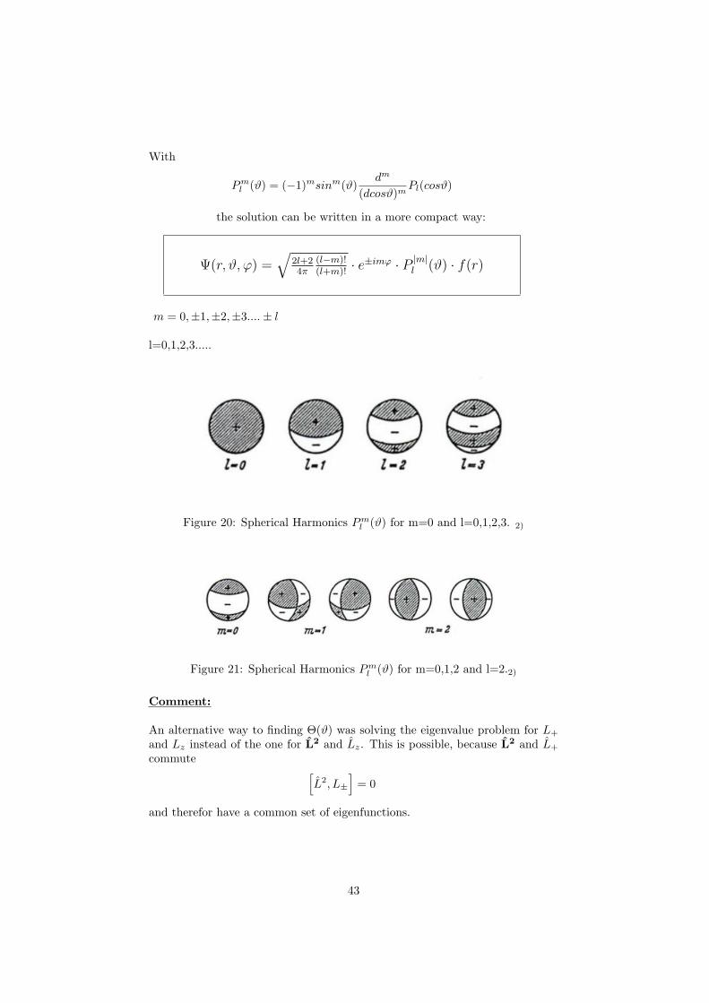
Figure 20: Spherical Harmonics Pml (ϑ) for m=0 and l=0,1,2,3. 2)
Figure 21: Spherical Harmonics Pml (ϑ) for m=0,1,2 and l=2.2)
Comment:
An alternative way to finding Θ(ϑ) was solving the eigenvalue problem for L+
and Lz instead of the one for L2 and Lz. This is possible, because L2 and L+
commute [L2, L±
]= 0
and therefor have a common set of eigenfunctions.
43
Back to equation (76):
Comparison of L2 and ∆ϑϕ in spherical coordinates shows, that eq.(76) can bewritten as
L2
2mr2Ψ(r, ϑ, ϕ) = EΨ(r, ϑ, ϕ)
Since the eigenvalue problem for L2 was solved above and 12mr2 = const., the
wavefunction and energy eigenvalues for electrons 0n the surface of a sphereare
Ψ(r, ϑ, ϕ) =√
2l+24π√%
(l−m)!(l+m)!
· e±imϕ · P |m|l (ϑ) · δ(r − %)
E = ~2
2mr2l(l + 1)
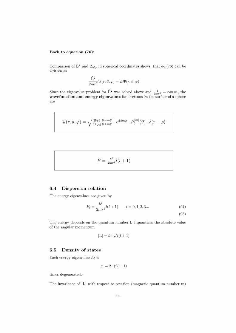
6.4 Dispersion relation
The energy eigenvalues are given by
El =~2
2mr2l(l + 1) l = 0, 1, 2, 3... (94)
(95)
The energy depends on the quantum number l. l quantizes the absolute valueof the angular momentum.
|L| = ~ ·√l(l + 1)
6.5 Density of states
Each energy eigenvalue El is
gl = 2 · (2l + 1)
times degenerated.
The invariance of |L| with respect to rotation (magnetic quantum number m)
44
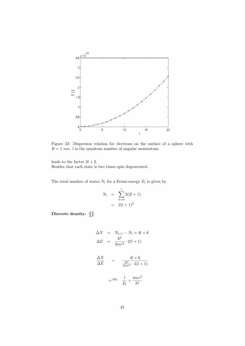
Figure 22: Dispersion relation for electrons on the surface of a sphere withR = 1 nm. l is the quantum number of angular momentum.
leads to the factor 2l + 2.Besides that each state is two times spin degenerated.
The total number of states Nl for a Fermi-energy El is given by
Nl =l∑
k=0
2(2l + 1).
= 2(l + 1)2
Discrete density: ∆N∆E
∆N = Nl+1 −Nl = 4l + 6
∆E =~2
2mr2· 2(l + 1)
∆N∆E
=4l + 6
~2
2mr2 · 2(l + 1)
=(94) l
El+
4mr2
~2
45
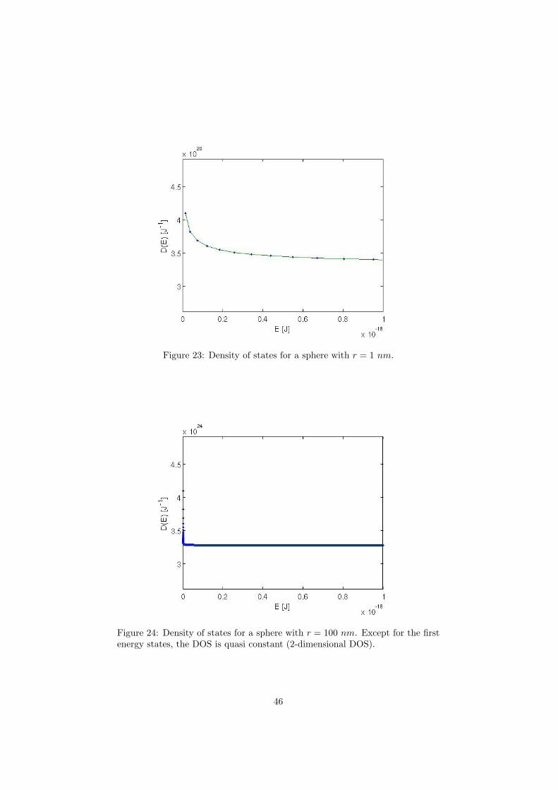
Figure 23: Density of states for a sphere with r = 1 nm.
Figure 24: Density of states for a sphere with r = 100 nm. Except for the firstenergy states, the DOS is quasi constant (2-dimensional DOS).
46
6.6 Program
The dispersion relation and the density of states were studied with Matlab: theprogram sphere.m will ask for the radius and show the dispersion relation andthe density of states for the chosen radius.
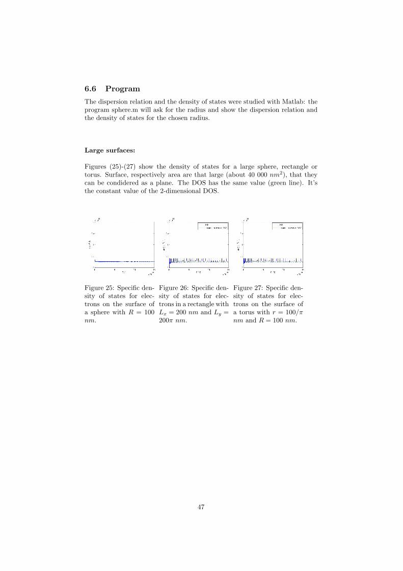
Large surfaces:
Figures (25)-(27) show the density of states for a large sphere, rectangle ortorus. Surface, respectively area are that large (about 40 000 nm2), that theycan be condidered as a plane. The DOS has the same value (green line). It’sthe constant value of the 2-dimensional DOS.
Figure 25: Specific den-sity of states for elec-trons on the surface ofa sphere with R = 100nm.
Figure 26: Specific den-sity of states for elec-trons in a rectangle withLx = 200 nm and Ly =200π nm.
Figure 27: Specific den-sity of states for elec-trons on the surface ofa torus with r = 100/πnm and R = 100 nm.
47
7 Appendix
Nabla operator in cylindrical coordinates:
∆ =1r
δ
δr
(rδ
δr
)+
1r2
δ2
δϕ2+
δ2
δz2
=δ2
δr2+
1r
δ
δr+
1r2
δ2
δϕ2+
δ2
δz2(96)
Nabla operator in spherical coordinates:
∆ =1r2
δ
δr
(r2 δ
δr
)+
1r2sinθ
δ
δϑ
(sinθ
δ
δθ
)+
1r2
1sin2θ
δ2
δϕ2(97)
hermetian:
A matrix is hermetian if
A = A† (98)
A† means to transpone and complex conjugate (or vice versa) the matrix:
A† = (AT )∗ = (A∗)T
It’s the analogy of a real space symmetric matrix but in complex space.Hermitesh matrices are square, normal and diagonalisable.
Since each Operator in an n dimensional vector space can be described by annXn matrix, one can also call an operator hermetian:
A = A†
A quantum mechanical postulate says, that each physical observable (f. i. en-ergy, position, angular momentum) formally corresponds to a hermetian opera-tor:
48
A =∑j
aj |aj >< aj | (99)
Hermitesh operators
• work the same way on Bra- and Ket-vectors.
• have real eigenvalues
• eigenvectors to different eigenvalues are orthogonal
• if the eigenvalues are degenerated it’s always possible to chose them to beorthogonal
• the eigenvectors build a basis, a complete set of eigenstates.
49
8 Literature
[1] Nolting, Wolfgang: Grundkurs theoretische Physik 5/2, Quantenmechanik-Methoden und Anwendungen,4.Auflage, Springer Berlin [u.a.], 2004,ISBN:3-540-4211-4
[2] Flugge, Siegfried: Rechenmethoden der Qauntenmechanik,6.Auflage, SpringerBerlin [u.a.], 1999, ISBN:3-540-65599-9
[3] Claude Cohen-Tannoudji, Bernard Diu, Franck Laloe: Quantum Mechan-ics,vol.1 and 2, 2.edition, Hermann and John Wiley and Sons, Paris, New York[a.o.] 1977, ISBN: vol.1: 2-7056-5833-5 (Hermann), vol.2: 2-7056-5834-3
[4] Kittel, Charles: Introduction to solid state physics, 8.edition, Wiley, NewYork [a.o.] 2005, ISBN:978-0-471-41526-8
[5] Bartsch, Hans-Jochen: Taschenbuch mathematischer Formeln, 20.Auflage,Fachbuchverlag Leipzig im Carl Hanser Verlag, Munchen Wien 2004, ISBN:3-446-22891-8
[6] Moon P., Spencer D. : Field theory handbook, Springer, Berlin [u.a.] 1961
[7] Morse Ph., Feshbach : Methods of theoretical physics,vol.1 and 2,McGraw-Hill Book Company, Inc., New York [a.o] 1953 ISBN: vol.1: 0-07-043316-X,vol.2: 0-07-043317-8
[8] Arfken, George B.: Mathematical methods for physicists, 4. edition, Acad.Press, San Diego, California [u.a.] 1999, ISBN:0-12-059816-7
Articles:
[9] Han, Jie: Toroidal Single Wall Carbon Nanotubes in Fullerene Crop Circleshttp://www.nas.nasa.gov/News/Techreports/1997/PDF/nas-97-015.pdf, 31.05.2008
[10] Liu, Jie [a.o.]:’Fullerene Crop Circles’, In: Scientific Correspondencehttp://www.nas.nasa.gov/News/Techreports/1997/PDF/nas-97-015.pdf
50
Articles from the Internet:
[11] http://de.wikipedia.org/wiki/Zustandsdichte, 03/03/2009
[12] http://britneyspears.ac/physics/dos/dos.htm, 03/03/2009
[13] http://www.technologyreview.com/computing/22257, 19/03/2009
51
%RECTANGLE
%dispersionrelation and density of states
clcclear allclose allc
h=6.6261*10^(-34); %in Jsm=9.11*10^(-31); %in kg
F=(h/2/pi).^2./(2*m);
disp('Choose a length Lx in meters');Lx=input('Lx=');
if isempty(Lx)Lx=1e-9;fprintf('%e',Lx)ende
r=Lx/(2*pi);r
fprintf('\n')fprintf('\n')fprintf('\n')disp('Choose a ratio Ly/Lx>1');fprintf('\n')ff
ratio=input('Ly/Lx=');fprintf('\n')f
if ratio<1 %necessary for the formula of the DOSdisp('Invalid value for the ratio! Choose Ly/Lx>1')fprintf('\n')ratio=input('Ly/Lx=')ende
if isempty(ratio)ratio=2;fprintf('%e',ratio)endeeee
R=ratio*r;
Ly=2*R*pi;L
A=Lx*Ly; %Area of the rectangle
nR=[1:ratio*50]; nphi=[1:50];
[nR,nphi ]=meshgrid(nR,nphi);E_nR=nR.^2./R.^2.*F; %eigenvalues for nphi=0E_nphi= nphi.^2./r.^2.*F; %eigenvalue for nR=0
En=E_nR +E_nphi; %energy eigenvalues
figure(1)set(0,'DefaultAxesFontSize',12)z_par=5; %number of parabolassubplot(1,2,1)s
for i=1:z_par plot([0,1],[E_nphi(i,1),E_nphi(i,1)])hold onendhold offtitle('E_n_x','FontSize', 12)xlabel('[1]','FontSize', 12)ylabel('E_n_x [J]','FontSize', 12)axis([0 1 -1/8*E_nphi(z_par,1) (9/8)*E_nphi(z_par,1)])
subplot(1,2,2) s
for i=1:z_parplot([0,1],[E_nR(1,i),E_nR(1,i)])hold onendhold offh
title('E_n_y','FontSize', 12)xlabel('[1]','FontSize', 12)ylabel('E_n_y [J]','FontSize', 12)
axis([0 1 -1/8*E_nphi(z_par,1) (9/8)*E_nphi(z_par,1)])
%DISP%
figure(2) f
%dispersionsrelation E(n_phi,n_R) over n_Rx=nR(1,:);y=En;y
for i=1:size(En,1)plot(x,y(i,:),'Color',[0,1,0])hold onplot(x,y(i,:),'.')hold onendhold offh
title('dispersion relation for a rectangle','FontSize', 12)xlabel('n_x [1]','FontSize', 12)ylabel('E_n_x,n_y [J]','FontSize', 12)
%DOS%
nR=nR(1,:);nphi=nphi(:,1)';E_nR=E_nR(1,:);E_nphi=E_nphi(:,1)';
%quasicontinuous 1d-single-DOS
E=linspace(En(1,2),En(end,end),90000);[E,El]=meshgrid(E,E_nphi);
D_1=(sqrt(2*m)*8*pi*R/h).*heaviside(E-El)./(sqrt(E-El));D_1((E-El)==0)=0; %problem:1/0
plotend=sum(D_1(end,:)~=0);
if plotend==size(E,2)plotend=0end
D_1sum=sum(D_1,1);
%quasicontinuous 2d-DOS
D_2=16*pi^3*m*R*r/(h^2);
figure(3)set(0,'DefaultAxesFontSize',12)
%D_1sum(D_1sum> c )=c ; %c= cut off the infinite values
plot([E(1,1),E(1,1:(end-plotend))],[0,D_1sum(1:(end-plotend))])hold onplot([E(1,1),E(1,end-plotend)],[D_2,D_2], 'Color',[0,1,0])hold offlegend('DOS','constant value of 2d DOS','FontSize',20)title('Density of states for a rectangle','FontSize', 14)xlabel('E [J]','FontSize', 12 )ylabel('D(E) [J^-1]','FontSize', 12)
%specific density of states (DOS per unit area)
d=D_1sum./A;d2=D_2./A;d
figure(4)set(0,'DefaultAxesFontSize',12)
%d(d> c)= c; %c= cut off the infinite values
plot([E(1,1),E(1,1:(end-plotend))],[0,d(1:(end-plotend))])hold onplot([E(1,1),E(1,end-plotend)],[d2,d2], 'Color',[0,1,0])hold offlegend('DOS','constant value of 2d DOS','FontSize',20)title('Specific density of states for a rectangle','FontSize', 14)xlabel('E [J]','FontSize', 12 )ylabel('d(E) [J^-1m^-2]','FontSize', 12)

%TORUS
%dispersionrelation and density of states
%
clcclear allclose all
c
h=6.6261*10^(-34); %in Jsm=9.11*10^(-31); %in kg
mm
F=(h/2/pi).^2./(2*m);
FFF
disp('Choose a radius r for the torus cross section in meters');r=input('r='); %radius of the torusring
r
if isempty(r)r=0.7e-9;fprintf('%e',r)end
ee
fprintf('\n')fprintf('\n')fprintf('\n')disp('Choose the ratio R/r >= 1');fprintf('\n')
ff
ratio=input('ratio=');
rr
if ratio<1disp('Invalid choice of ratio, ratio has to be >=1') r=input('r=');end
e
if isempty(ratio)ratio=2;fprintf('%e',ratio)end
eeee
R=ratio*r;
R
nR=[0:ratio*70]; nphi=[0:70];

A=4*pi^2*R*r; %surface of the torus
AA
%DISP [nR,nphi ]=meshgrid(nR,nphi);E_nR=nR.^2./R.^2.*F; %eigenvalues for nphi=0E_nphi= nphi.^2./r.^2.*F; %eigenvalues for nR=0
EE
En=E_nR +E_nphi; %energy eigenvalues
EEEE
figure(1)set(0,'DefaultAxesFontSize',12)z_par=5; %number of parabolassubplot(1,2,1)
s
for i=1:z_par plot([0,1],[E_nphi(i,1),E_nphi(i,1)])hold onendhold offtitle('E_n_\phi','FontSize', 12)xlabel('[1]','FontSize', 12)ylabel('E_n_\phi [J]','FontSize', 12)axis([0 1 -1/8*E_nphi(z_par,1) (9/8)*E_nphi(z_par,1)])
aa
subplot(1,2,2)
s
for i=1:z_parplot([0,1],[E_nR(1,i),E_nR(1,i)])hold onendhold off
h
title('E_n_\theta','FontSize', 12)xlabel('[1]','FontSize', 12)ylabel('E_n_\theta [J]','FontSize', 12)
y
axis([0 1 -1/8*E_nphi(z_par,1) (9/8)*E_nphi(z_par,1)])
aaaa
%DISP
figure(2) %dispersionsrelation E(n_phi,n_R) over n_Rset(0,'DefaultAxesFontSize',12)s
x=nR(1,:);y=En;y
for i=1:size(En,1)plot(x,y(i,:),'Color',[0,1,0])hold onplot(x,y(i,:),'.')hold onendhold offh
title('dispersion relation for a torus','FontSize', 12)xlabel('n_\theta [1]','FontSize', 12)ylabel('E_n_\theta,n_\phi [J]','FontSize', 12)axis([x(1) 100 En(1,1) En(1,100) ]) a
%DOS%
nR=nR(1,:);nphi=nphi(:,1)';n
E_nR=E_nR(1,:);E_nphi=E_nphi(:,1)';EE
%quasicontinuous 1d-single-DOS %
E=linspace(En(1,2),En(end,end),90000);[E,El]=meshgrid(E,E_nphi);[
D_1=(sqrt(2*m)*8*pi*R/h).*heaviside(E-El)./(sqrt(E-El));D_1((E-El)==0)=0; %problem: 1/0DDD
plotend=sum(D_1(end,:)~=0);p
if plotend==size(E,2)plotend=0ende
D_1sum=sum(D_1,1);D
xx
%(quasicontinuous DOS) 2d-DOS%
D_2=16*pi^3*m*R*r/(h^2); DD
figure(3)set(0,'DefaultAxesFontSize',12)s
%D_1sum(D_1sum> c )=c; %c= cut off the infinite values%%
plot([E(1,1),E(1,1:end-plotend)],[0,D_1sum(1:end-plotend)])hold onplot([E(1,1),E(1,end-plotend)],[D_2,D_2], 'Color',[0,1,0])hold offlegend('DOS','constant value of 2d DOS','FontSize',12)title('Density of states for a torus','FontSize', 12)xlabel('E [J]','FontSize', 12 )ylabel('D(E) [J^-1]','FontSize', 12)yyyyy
%specific density of states%
d=D_1sum ./A;d2=D_2 ./A;dd
figure(4)set(0,'DefaultAxesFontSize',12)ss
%d(d>c)=c; %c= cut off the infinite values%%
plot([E(1,1),E(1,1:end-plotend)],[0,d(1:end-plotend)])hold onplot([E(1,1),E(1,end-plotend)],[d2,d2], 'Color',[0,1,0])hold offlegend('DOS','constant value of 2d DOS','FontSize',12)title('Specific density of states for a torus','FontSize', 12)xlabel('E [J]','FontSize', 12 )ylabel('d(E) [J^-1m^-2]','FontSize', 12)y
%SPHERE
%dispersionrelation and density of states
clcclear allclose all
c
h=6.6261*10^(-34); %in Jsm=9.11*10^(-31); %in kg
m
l=[0:400];R=input('Value for the radius R=');if isempty(R) R=1e-9end
ee
F=(h/(2*pi))^2./(2.*m.*R.^2);
F
E=F.*l.*(l+1); %energy eigenvalues
E
A=4*pi*R^2; %surface of a sphere
AAA
%DISP
%
figure(1)
f
set(0,'DefaultAxesFontSize',12)
s
plot(l,E,'.',l,E)title('Dispersion relation')xlabel('Drehimpulsquantenzahl l','FontSize', 12)ylabel('E [J]','FontSize', 12)
%DOS
%
D=l./E+(16*pi^2*m*R^2/h^2);
D
figure(2)set(0,'DefaultAxesFontSize',12)
s
plot(E,D,'.',E,D)title('Density of states','FontSize', 12)xlabel('E [J]')ylabel('D(E) [J^-1]','FontSize', 1)
y
ááá
%specific density of states (DOS per unit area)
%
d=D./A;
d
figure(3)set(0,'DefaultAxesFontSize',12)
s
plot(E,d,'.',E,d)title('Specific density of states for a spherical shell','FontSize', 12)xlabel('E [J]')ylabel('d(E) [J^-1m^-2]','FontSize', 1)