REPORT OF INVESTIGATION 25

STATE OF ILLINOIS

OTTO KERNER, Governor

DEPARTMENT OF REGISTRATION AND EDUCATION

WILLIAM SYLVESTER WHITE, Director

Selected Methods for Pumping Test Analysis

by JACK BRUIN and H. E. HUDSON JR.

ILLINOIS STATE WATER SURVEY

WILLIAM C.ACKERMANN, Chief

URBANA

Third Printing, 1961

REPORT OF INVESTIGATION 25

STATE OF ILLINOIS

OTTO KERNER, Governor

DEPARTMENT OF REGISTRATION AND EDUCATION

WILLIAM SYLVESTER WHITE, Director

SELECTED METHODS FOR PUMPING TEST ANALYSIS

by JACK BRUIN and H. E. HUDSON, JR.

STATE WATER SURVEY DIVISION

WILLIAM C. ACKERMANN, Chief

URBANA

First Printing, 1955

Second Printing, 1958

Third Printing, 1961

TABLE OF CONTENTS Page

SUMMARY 5

INTRODUCTION 6 Scope of Report 6 Acknowledgments 6

GENERAL 6 Historical 6 System of Units 7

NON-EQUILIBRIUM METHOD 8 Analysis of Test Data 8

Type Curve Solution 8 Example of Analysis 11

Estimation of Future Pumping Water Levels 16

MODIFIED NON-EQUILIBRIUM METHOD 17 Analysis of Test Data 17

Drawdown Method 17 Recovery Method 19

Estimation of Future Pumping and Non-Pumping Water Levels 19 Self-caused Drawdown 21 Interference 21 Areal Recession 22 The Future Pumping and Non-Pumping Water Levels 22

AQUIFER OF LIMITED AREAL EXTENT 22 Hydrologic Boundaries 22

Example of Analysis 26 Recharge Boundaries 27

STEP DRAWDOWN TESTS 29 General Discussion 29 Example of Analysis 30

COMPLICATING FACTORS 36

REFERENCES 38

APPENDIX I 39

APPENDIX II 47 Introduction 49 The Pumped Well 49 Pumping Equipment 50 Observation Wells 50 Period Prior to Test 50 Notes Concerning Collection of Data 50 Types of Pumping Tests 51

5

SUMMARY

The report describes and illustrates four types of pumping test data analysis which at present are exten­sively used in analysis of problems involving Illinois wells. These methods are, the non-equilibrium "type curve" method, the modified non-equilibrium "straight l ine" method, the step-drawdown analysis developed by Water Survey staff members, and the analysis of an aquifer that has limited areal extent.

The pumping test is one of the most useful tools avail­able in the evaluation of groundwater producing forma­tions. The material in this report is designed to meet the present needs of engineers who deal with groundwater in Illinois. So far as possible the details of theories involved have been omitted. Substituted for them are general dis­cussions of the applicability of the various types of analy­sis. Attention is called to the advantages, disadvantages

and possible mis-use of the equations presented. The assumptions upon which the various types of analysis are based are also discussed.

The "type curve" method is of particular value when observation wells are available and the aquifer being tested is of large areal extent and when the pumping test is of too short duration to use the straight-line meth­od. The "straight l ine" method is applicable when ob­servation wells are available and when the testing period is sufficiently long to warrant its use. The analysis of an aquifer of limited areal extent is an adaptation of the "straight l ine" method to meet the conditions when one or more boundaries of the aquifer are in the vicinity of the well being pumped. The step-drawdown analysis yields information primarily concerning the performance of the well itself rather than the aquifer and does not usually require observation wells.

6

SELECTED METHODS FOR GROUNDWATER RESOURCES EVALUATION

By Jack Bruin, Assistant Engineer

and H. E. Hudson Jr., Head, Engineering Sub-Division

Illinois State Water Survey Division, Urbana, Illinois

INTRODUCTION

Scope of Report

This report presents elements of established pumping test analysis procedure which are valuable and beneficial to professional and practicing engineers, well contractors and drillers, municipal and industrial operators, and others interested in the future planning and development of groundwater resources. The report includes a limited number of cases for which well-substantiated clear-cut solutions could be worked out. This report contains ref­erences to the literature germane to those cases.

The derivations and proofs of equations have been eliminated. The equations are presented in their devel­oped form with a discussion of their applicability and shortcomings. An example of each method is presented

by analyzing an actual pumping test that was not com­plicated by recharge considerations.

Acknowledgments

The suggestions and constructive criticisms of Mr. H. F. Smith, Engineer, State Water Survey Division, were of great value in the preparation of this report.

The authors are indebted to the engineers of the State Water Survey Division who have collected data from ap­proximately 1300 pumping tests during the past 20 years.

The writers are especially indebted to Mr. Francis X. Bushman, formerly Assistant Engineer, State Water Survey Division, for his work in preparing the Historical section.

GENERAL

Historical

The analysis of the hydraulics of wells for the evalu­ation of groundwater potentialities by pumping tests falls in the category of groundwater hydrology. This field has been rapidly developed since the publication of the well-known law of flow through porous materials by Henri Darcy in 1856. (1)* This law states that the discharge through porous media is proportional to the product of the hydraulic gradient, the cross-sectional area normal to the flow and the coefficient of permeability of the material.

In 1863, Dupuit(2) applied Darcy's law to well hy­draulics, using an ideal case of a well located at the center of a circular island.

The Dupuit formula was modified by Thiem ( 3 ) in 1906 to a form which is applicable to more general problems. Similar formulas were also advanced by Slichter(4), Turneaure and Russell(5), Israelson(6), Muskat(7), and Wenzel (8). However, all of these were essentially either modified or specialized forms of Dupuit's relationship. These methods may all be classed together as the "equi­librium method'' which applies only to a steady-state condition in which the rate of flow of water toward the well is equal to the rate of discharge of the pumped well.

A remarkable advance in modern well hydraulics was made through the development of the non-equilibrium theory by Theis (9) of the U. S. Geological Survey in 1935. This theory introduced the time factor and the co-

*Numbers refer to the list of references on page 34.

efficient of storage; it made possible the computation of future pumping levels when the flow of groundwater due to pumping did not approach an equilibrium condition.

However, the use of the Theis formula in determining the coefficients of transmissibility and storage-the for­mation constants of an aquifer- presented much difficulty because of mathematical complexities in applying the formula, which contains an exponential integral. Theis suggested a graphical method to Wenzel(10) and Jacob(11), respectively, in 1937 and 1938, for a more practical so­lution of this problem. The method was described by Jacob in 1940 and by Wenzel in 1942.

In 1944, Wenzel and Greenlee(12) presented a gener­alization of Theis' graphical solution by which the co­efficients may be determined from tests of one or more discharging wells operated at varied rates.

Furthermore, Cooper and Jacob (13) have introduced an approximation into the non-equilibrium method which results in a method which is convenient to use.

Both the equilibrium and the non-equilibrium methods assume that the water-bearing material is homogeneous and isotropic. This assumption is probably never true in a natural aquifer. However, these methods give reliable results in actual cases when there is no hydrologic boun­dary existing within the effective area of pumping. Ex­tended application of the equilibrium method to the problems involving hydrologic boundaries was made by Muskat(14) in 1937 by the method of images.

In 1941, Theis(15) illustrated the application of his non-equilibrium formula to a special boundary problem in which the effect of a well on the flow of a nearby

7

stream was considered.

In 1948, Ferris(16) applied the method of images in the use of the non-equilibrium theory to the general treatment of simple boundary problems.

The Illinois State Water Survey became very active in promoting production tests of wells during the early 1920's. Much of this promotion work was done by per­sonal contact with water well contractors, consulting engineers, and municipal officials. As a result numerous measurements of production rates and water levels for individual wells became available. Under the leadership of the late G. C. Habermeyer, Engineer of the Survey, the use of electric droplines for water level measurements became standard practice for Survey engineers prior to 19259.(24)

For the period 1920-30, Water Survey records reveal eight pumping tests conducted by Survey personnel. The total number of pumping tests on record in the Survey files through 1954 is 1,321.

The first test on record in the Survey files by Survey personnel was conducted on a municipal well at Lawr-enceville in 1922.

The Illinois State Water Survey has used the method of images, based on Ferris' procedure, in a number of cases where the data indicated the existence of boundary conditions, either impermeable or recharge, and in a few cases where both effects were observed.

The Survey has used the non-equilibrium method and most of its modifications in approximately half of the pumping tests conducted since 1946, all of which involved the estimation of future conditions. While making these analyses the characteristics of individual wells have also been studied.

Survey engineers have made a thorough review of the literature on the subject. Much of it pertains to cases for which good examples have not been encountered in Illinois.

The importance and need of this phase of science becomes apparent when one notes the great number of water uses. No living thing exists without water. Noting the progress of groundwater hydrology in the past 20 years or so one may hold forth great hope for future develop­ments and expansions of existing facilities.

System of Units

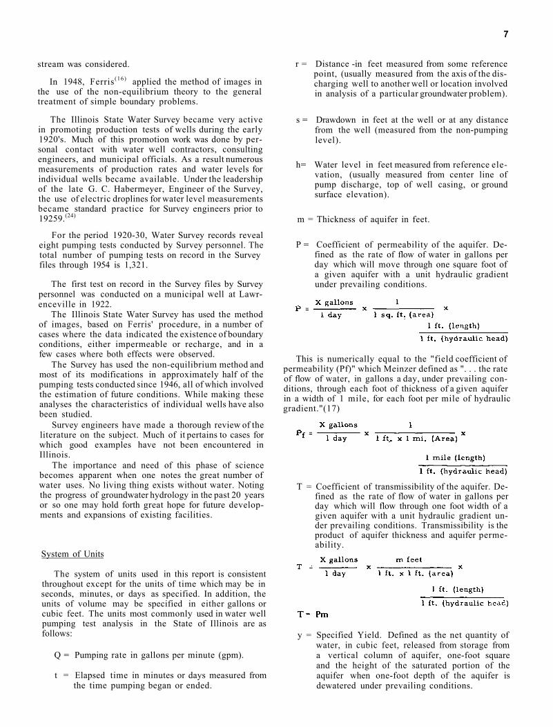
The system of units used in this report is consistent throughout except for the units of time which may be in seconds, minutes, or days as specified. In addition, the units of volume may be specified in either gallons or cubic feet. The units most commonly used in water well pumping test analysis in the State of Illinois are as follows:

Q = Pumping rate in gallons per minute (gpm).

t = Elapsed time in minutes or days measured from the time pumping began or ended.

r = Distance -in feet measured from some reference point, (usually measured from the axis of the dis­charging well to another well or location involved in analysis of a particular groundwater problem).

s = Drawdown in feet at the well or at any distance from the well (measured from the non-pumping level).

h= Water level in feet measured from reference ele­vation, (usually measured from center line of pump discharge, top of well casing, or ground surface elevation).

m = Thickness of aquifer in feet.

P = Coefficient of permeability of the aquifer. De­fined as the rate of flow of water in gallons per day which will move through one square foot of a given aquifer with a unit hydraulic gradient under prevailing conditions.

This is numerically equal to the "field coefficient of permeability (Pf)" which Meinzer defined as ". . . the rate of flow of water, in gallons a day, under prevailing con­ditions, through each foot of thickness of a given aquifer in a width of 1 mile, for each foot per mile of hydraulic gradient."(17)

T = Coefficient of transmissibility of the aquifer. De­fined as the rate of flow of water in gallons per day which will flow through one foot width of a given aquifer with a unit hydraulic gradient un­der prevailing conditions. Transmissibility is the product of aquifer thickness and aquifer perme­ability.

y = Specified Yield. Defined as the net quantity of water, in cubic feet, released from storage from a vertical column of aquifer, one-foot square and the height of the saturated portion of the aquifer when one-foot depth of the aquifer is dewatered under prevailing conditions.

8

S = Coefficient of storage. Defined as the net quan­tity of water in cubic feet released from storage from a vertical column of aquifer, one-foot

square and the height of the saturated portion of the aquifer, when the hydraulic pressure on the column is reduced one-foot of water under pre­vailing conditions.

For water table conditions, S = y.

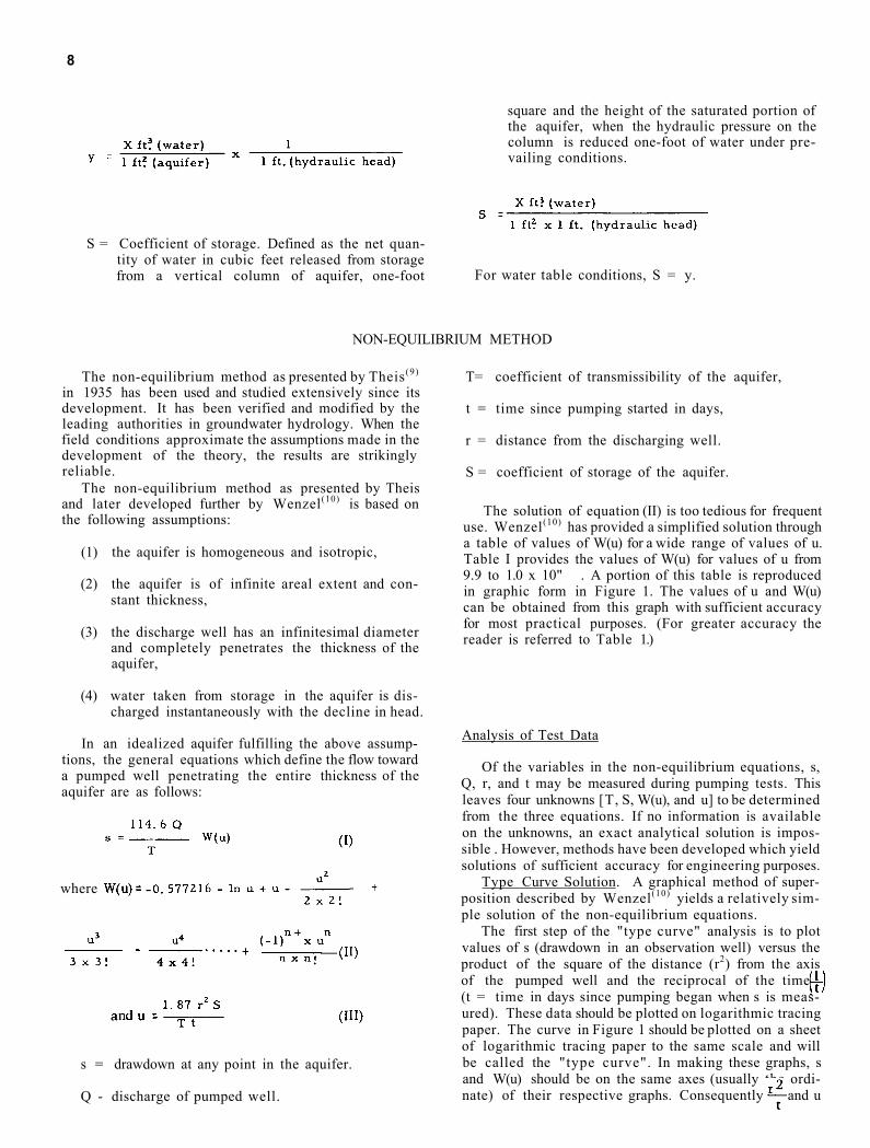
NON-EQUILIBRIUM METHOD

The non-equilibrium method as presented by Theis (9)

in 1935 has been used and studied extensively since its development. It has been verified and modified by the leading authorities in groundwater hydrology. When the field conditions approximate the assumptions made in the development of the theory, the results are strikingly reliable.

The non-equilibrium method as presented by Theis and later developed further by Wenzel(10) is based on the following assumptions:

(1) the aquifer is homogeneous and isotropic,

(2) the aquifer is of infinite areal extent and con­stant thickness,

(3) the discharge well has an infinitesimal diameter and completely penetrates the thickness of the aquifer,

(4) water taken from storage in the aquifer is dis­charged instantaneously with the decline in head.

In an idealized aquifer fulfilling the above assump­tions, the general equations which define the flow toward a pumped well penetrating the entire thickness of the aquifer are as follows:

where

s = drawdown at any point in the aquifer.

Q - discharge of pumped well.

T= coefficient of transmissibility of the aquifer,

t = time since pumping started in days,

r = distance from the discharging well.

S = coefficient of storage of the aquifer.

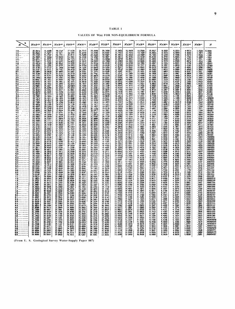
The solution of equation (II) is too tedious for frequent use. Wenzel(10) has provided a simplified solution through a table of values of W(u) for a wide range of values of u. Table I provides the values of W(u) for values of u from 9.9 to 1.0 x 10" . A portion of this table is reproduced in graphic form in Figure 1. The values of u and W(u) can be obtained from this graph with sufficient accuracy for most practical purposes. (For greater accuracy the reader is referred to Table 1.)

Analysis of Test Data

Of the variables in the non-equilibrium equations, s, Q, r, and t may be measured during pumping tests. This leaves four unknowns [T, S, W(u), and u] to be determined from the three equations. If no information is available on the unknowns, an exact analytical solution is impos­sible . However, methods have been developed which yield solutions of sufficient accuracy for engineering purposes.

Type Curve Solution. A graphical method of super­position described by Wenzel(10) yields a relatively sim­ple solution of the non-equilibrium equations.

The first step of the "type curve" analysis is to plot values of s (drawdown in an observation well) versus the product of the square of the distance (r2) from the axis of the pumped well and the reciprocal of the time (t = time in days since pumping began when s is meas­ured). These data should be plotted on logarithmic tracing paper. The curve in Figure 1 should be plotted on a sheet of logarithmic tracing paper to the same scale and will be called the "type curve". In making these graphs, s and W(u) should be on the same axes (usually the ordi­nate) of their respective graphs. Consequently and u

9

TABLE 1

VALUES OF W(u) FOR NON-EQUILIBRIUM FORMULA

(From U. S. Geological Survey Water-Supply Paper 887)

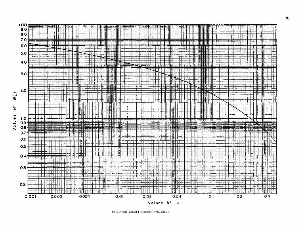
FIG. 1. A PORTION OF THE THEIS TYPE CURVE

11

would be on the same axes (usually the abscissa) of their respective graphs. The "type curve" should consist of a smooth curve while the pumping test data curve (s vs ) should consist of only the plotted individual points.

The next step is to place one of the graphs on top of the other and fit the points of the graph to the type curve. This can easily be done with the use of an illumi­nated tracing table. If numerous analyses are to be made, it is convenient to have a permanent "typecurve" con­structed on transparent material. For accurate work, the minimum size for the permanent type curve should cor­respond to 11 × 17 inch 5 × 3 cycle logarithmic graph paper. In fitting the plotted data to the type curve the coordinate axes of the two graphs must be kept parallel. When the "best fit" is obtained by eye, a "match-point" is selected, at any point desired on the fitted curve and

marked on both curves. The values of s, W(u), and u

to be used in calculating T and S are the values obtained from the "match-point" of the graphs. The values of T and S are computed from equations (I) and (III) in the following forms:

where s, Q, T, t, r, and S are as defined above. The following illustrative analyses will make this

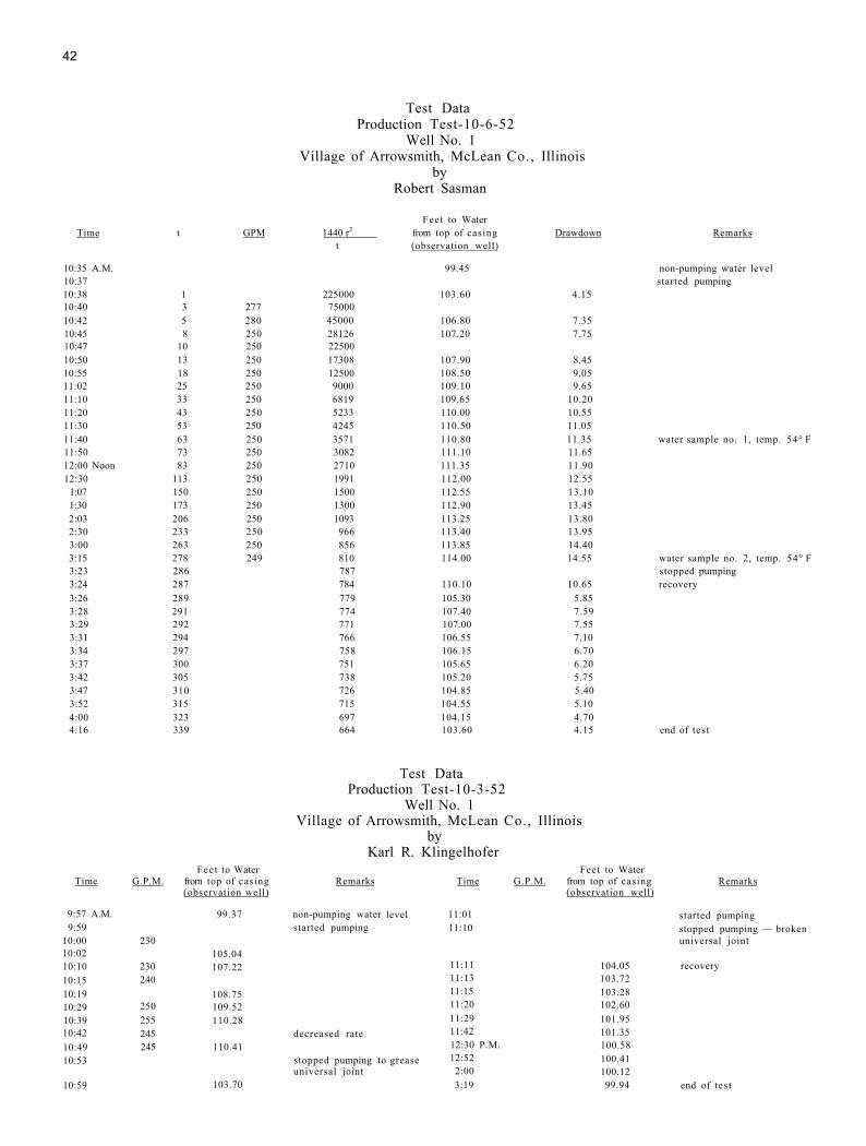
procedure clear. Example of Analysis. The well production test report

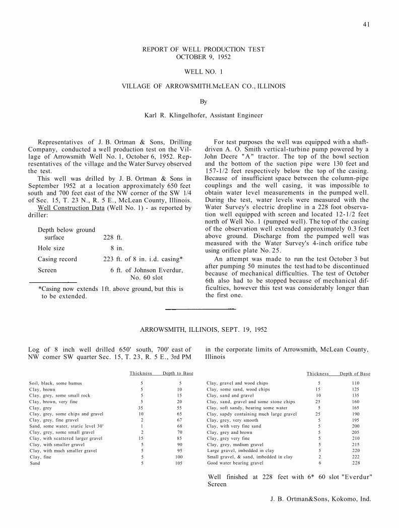
dated October 9, 1952 for Well No. 1 at the Village of Arrowsmith, Illinois presents the details of the well con­struction and the pumping test data (See Appendix II).

It should be noted that it was not possible to measure the water levels in the pumped well but water levels were measured in an observation well 12.5 feet away. The data from the test should make it possible to calcu­late the values of the formation constants (T and S) and to estimate the future water level recessions in the vicin­ity of the well that would result from pumping the well at various rates. The water level in the well cannot be predicted from these data with precision since the obser­vation well data do not reflect the head lost by the water as it enters the well and flows up the well to the pump intake (known as well loss).

The first step in the analysis of the data involves simple calculations. Determine the time in minutes (t) after pumping began at which each water level observa­tion was made. Square the distance (r 12.5) from the pumped well and divide it by the time in days at which the water level observations were made. Since there are 1440 minutes in a day this latter calculation becomes

, Next, determine the drawdown, which is the

water level in the observation well at the time of each observation minus the level before pumping began, i.e. the amount the water has lowered in the observation well since pumping began. The results of these calculations are shown on the test data sheet of the October 6 test in Appendix II. The next step is to plot the values of

versus the drawdown for each value of t on log­arithmic graph paper. On another sheet of similarpaper, plot a "type curve" of the values of W(u) and (u) de­rived from Table I. Figure 1 is a segment of the "type curve".

Compare the plotted test data with the type curve by a suitable method that permits placing one sheet of pa­per on top of the other so that plottings on both sheets may be seen simultaneously. Place the sheet with the plotted test data on top of the "type curve" with the

axis parallel to the u-axis and the drawdown

s-axis parallel to the W(u)-axis. The top sheet is shifted (always being careful to keep the axes parallel) until the plotted points of the test data are matched up with the "type curve" to make the best possible "eye fit" of the type curve through the plotted points of the test data. It is now usually advisable to trace that portion of the "type curve'' which fits the test data on the data sheet in order to keep a record of the fit obtained. While both sheets are still in this "best fit" position a "match-point" is chosen on the "best fit" portion of the " type curve" and marked. From this match point, record from the test data

sheet corresponding values of and drawdown and,

from the type curve, corresponding values of W(u) and u. The results of this procedure are illustrated in Figure 2.

Knowing the constant pumping rate of the test to be 250 gallons per minute, everything needed to solve for T and S by means of equations (I a) and (III a) is now available.

F r o m Figure 2, W(u) = 5 . 6 , u = 0. 002,

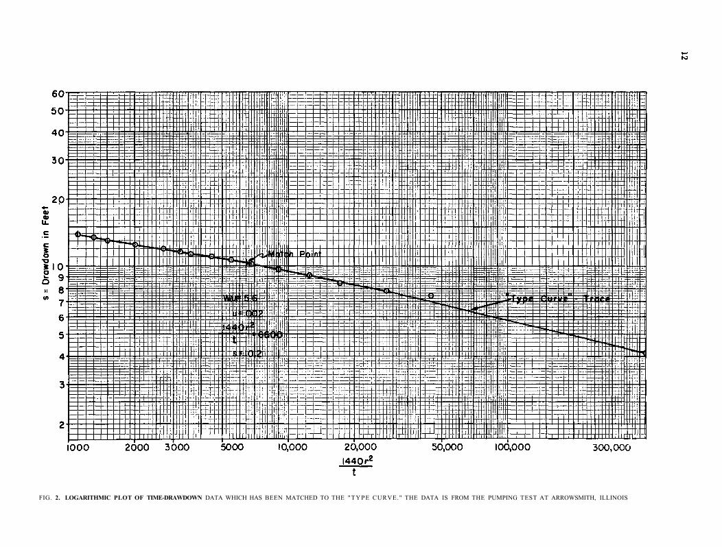
FIG. 2. LOGARITHMIC PLOT OF TIME-DRAWDOWN DATA WHICH HAS BEEN MATCHED TO THE "TYPE CURVE." THE DATA IS FROM THE PUMPING TEST AT ARROWSMITH, ILLINOIS

Knowing T and S it is now possible to use equations (I) and (III) to estimate the future water levels at any distance (r) from the pumped well and at any time (t) after pumping starts.

For example, assume the anticipated pumping sched­ule will require an average pumpage of 200 gpm for the first year at which time the rate would be increased to 300 gpm until the fifth year when a maximum antici­pated pumpage of 350 gpm would be reached. It is de­sired to know what the pumping level will be at the end of ten years.

The problem is approached in the following manner. Calculate the theoretical water levels at various distances from the well at various times and rates. In this case the calculations were made for the following convenient conditions, using the original pumpage and the incre­mental increases in pumping rates.

times - 1 day, 365 days, 1825 days, 3650 days

pumping rates - 50 gpm, 100 gpm, 200 gpm

distances - 1 ft, 10 ft, 100 ft, 1000 ft

time = 1 day

Q = 50 gpm from equation (III), u-

In equation (I b) S50 is the drawdown for a pumping rate of 50 gallons per minute. In equation (I b) the value of W(u) is dependent on the value of (u) which in turn depends on the values of (r) and (t). The constant 2.74 is dependent on the pumping rate. Therefore, in order to obtain the drawdown at other pumping rates equation (I b) need only be multiplied by the ratio of the desired pumping rate to 50 gpm. Thus for a pumping rate of 100 gpm:

13

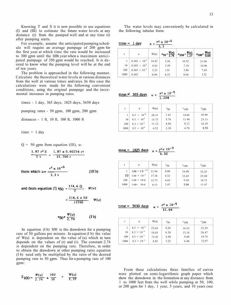
The water levels may conveniently be calculated in the following tabular form:

r

1

u

0.303 × 10-6

W(u)

14.42 5.26 10.52 21.06 10 0.303 × 10-4 9.83 3.59 7.18 -14.46

100 0.303 × 10 - 2 5.23 1.91 3.86 7.69 1000 0.303 0.90 0.33 0.66 1.32

r u W(u) S50 S100 S200

1 8.3 × 10-10 20.33 7.42 14.84 29.90

10 8.3 × 10-8 15.73 5.74 11.48 23.13

100 8.3 × 10 - 6 11.12 4.06 8.12 16.35

1000 8.3 × 10-4 6.52 2.38 4.76 9.59

r u W(u) S50 S100 S200

1 1.66 × 1 0 - 1 0 21.94 8.00 16.00 32.25 10 1.66 × 10 - 8 17.34 6.32 12.65 25.48

100 1.66 × 10-6 12.73 4.65 9.30 18.73 1000 1.66× 10-4 8.13 2.97 5.94 11.97

r u W(u) S50 S100 S200

1 8.3 × 10-11 22.64 8.26 16.53 33.29 10 8.3 × 10 - 9 18.03 6.58 13.16 26.47

100 8.3 × 10 - 7 13.42 4.90 9.80 19.74

1000 8.3 × 10 - 5 8.82 3.22 6.44 12.97

From these calculations three families of curves were plotted on semi-logarithmic graph paper which show the drawdown in the formation at any distance from 1 to 1000 feet from the well while pumping at 50, 100, or 200 gpm for 1 day, 1 year, 5 years, and 10 years (see

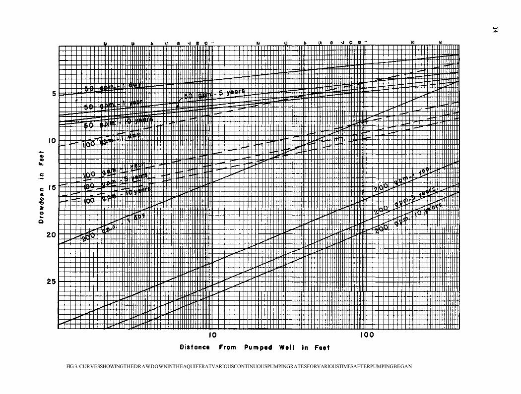
FIG. 3. CURVES SHOWING THE DRAWDOWN IN THE AQUIFER AT VARIOUS CONTINUOUS PUMPING RATES FOR VARIOUS TIMES AFTER PUMPING BEGAN

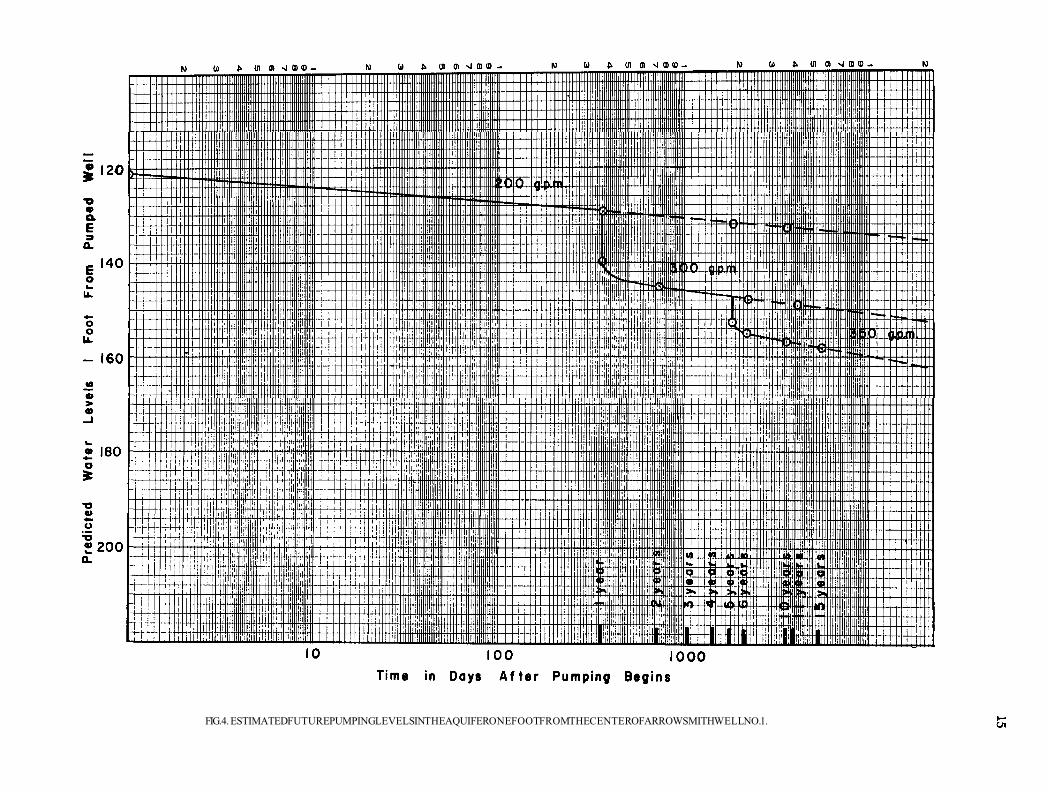
FIG. 4. ESTIMATED FUTURE PUMPING LEVELS IN THE AQUIFER ONE FOOT FROM THE CENTER OF ARROWSMITH WELL NO. 1.

16

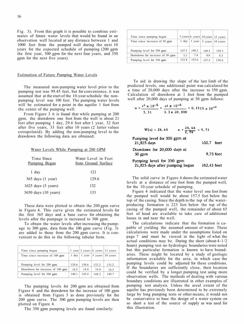
Fig. 3). From this graph it is possible to combine esti­mates of future water levels that would be found in an observation well located at any distance between 1 and 1000 feet from the pumped well during the next 10 years for the expected schedule of pumping (200 gpm the first year, 300 gpm for the next four years, and 350 gpm for the next five years).

Estimation of Future Pumping Water Levels

The measured non-pumping water level prior to the pumping test was 99.45 feet, but for convenience, it was assumed that at the start of the 10-year schedule the non-pumping level was 100 feet. The pumping water levels will be estimated for a point in the aquifer 1 foot from the center of the pumping well.

From Figure 3 it is found that while pumping at 200 gpm, the drawdown one foot from the well is about 21 feet after pumping 1 day, 29.6 feet after 1 year, 32 feet after five years, 33 feet after 10 years (2 latter values extrapolated). By adding the non-pumping level to the drawdown the following data are obtained:

Water Levels While Pumping at 200 GPM

Time Since Water Level in Feet Pumping Begun from Ground Surface

1 day 121

365 days (1 year) 129.6

1625 days (5 years) 132 3650 days (10 years) 133

These data were plotted to obtain the 200 gpm curve in Figure 4. This curve gives the estimated levels for the first 365 days and a base curve for obtaining the levels after the pumpage is increased to 300 gpm.

To obtain the water levels after increasing the pump-age to 300 gpm, data from the 100 gpm curve (Fig. 3) are added to those from the 200 gpm curve. It is con­venient to do this in the following tabular form.

Time since pumping began 1 year 2 years 6 years 11 years

Time since increase of 100 gpm 1 day 1 year 5 years 10 years

Pumping level for 200 gpm 129.6 130.6 132.2 133.2 Drawdown for increase of 100 gpm 10.5 14.8 16.0 16.5 Pumping level for 300 gpm 140.1 145.4 148.2 149.7

The pumping levels for 200 gpm are obtained from Figure 4 and the drawdown for the increase of 100 gpm is obtained from Figure 3 as done previously for the 200 gpm curve. The 300 gpm pumping levels are then plotted on Figure 4.

The 350 gpm pumping levels are found similarly:

Time since pumping began 5 years 6 years 10 years 15 years Time since increase of 50 gpm 1 day 1 year 5 years 10 years

Pumping level for 300 gpm 147.5 148.2 149.5 150.3 Drawdown for increase of 50 gpm 5.3 7.4 8.0 8.3 Pumping level for 350 gpm 152.8 155.6 157.5 158.6

To aid in drawing the slope of the last limb of the predicted levels, one additional point was calculated for a time of 20,000 days after the increase to 350 gpm. Calculation of drawdown at 1 foot from the pumped well after 20,000 days of pumping at 50 gpm follows:

The solid curve in Figure 4 shows the estimated water levels at a distance of one foot from the pumped well, for the 10-year schedule of pumping.

Figure 4 indicated that the water level one foot from the pumped well would be about 157.5 feet below the top of the casing. Since the depth to the top of the water-producing formation is 223 feet below the top of the casing of the pumped well, the remainder of about 65 feet of head are available to take care of additional losses in and near the well.

The calculations indicate that the formation is ca­pable of yielding the assumed amount of water. These calculations were made under the assumptions listed on page 7 and must be viewed in the light of what the actual conditions may be. During the short (about 4-1/2 hours) pumping test no hydrologic boundaries were noted but this particular formation is known to have bound­aries. These might be located by a study of geologic information available for the area, in which case the pumping levels could be adjusted for these conditions. If the boundaries are sufficiently close, their location could be verified by a longer pumping test using more observation wells. The methods of dealing with various boundary conditions are illustrated in other examples of pumping test analysis. Unless the areal extent of the aquifer has previously been determined to be extremely large by long pumping tests or other means, it would not be conservative to base the design of a water system on so short a test of the source of supply as was used for this illustration.

17

MODIFIED NON-EQUILIBRIUM METHOD

A very simple method for determining the formation coefficients was introduced by Cooper and Jacob ( 1 3 ) in 1946. It is a modification of the Thies non-equilibrium method. Cooper and Jacob have shown that when plotted on semi-logarithmic paper, the theoretical drawdown curve approaches a straight line when sufficient time has elapsed after pumping started.

In many instances plotting of the data while the test is in progress reveals whether the straight-line regime is being attained. However, the gentle transition into the straight line is sometimes hard to see without precise plotting and analysis, and may be confused with effects of other forces such as barometric effects, non-homo­geneity, variations in pumping rate, etc. The transition into the straight line may always be expected to occur but it may be hard to recognize because it sometimes passes very quickly and other times endures for an ex­tended period.

This modified method should yield coefficients with accuracy comparable to the type curve solution if the data used are from the portion of the pumping test after the values of u in equation (III) have become less than 0.01.

In equation (III), for any observation well located at a distance of r feet from a discharging well, the value of u becomes smaller as t becomes larger. Since at the time of testing, T and S are usually unknown, the prin­cipal difficulty in the use of this method is in estimating whether the pumping period has been long enough to yield enough data at values of u less than 0.01 for an accurate analysis. Frequently this can be determined by plotting the drawdown data versus the elapsed pumping time on semi-logarithmic graph paper (see Fig. 5) and noting whether the curve produced by the data approaches a straight line. However, occasionally the points may be curving so slightly as to deceive the analyst. If there is any doubt whatever of the validity of the solution, the "modified method" should be checked with the "type curve method." A detailed discussion of this problem was presented by Dr. Ven Te Chow in 1952.(19) Those who wish to pursue this aspect of the problem further are referred to the articles by Chow and by Cooper and Jacob.

Analysis of Test Data

From the portion of the data which plots as a straight line on semi-logarithmic graph paper, the formation coefficients may be determined by use of the following equations:

where:

T = Coefficient of transmissibility, Q = Pumping rate in gpm,

Δs = The change in drawdown in feet per log cycle in the straight-line portion of the drawdown curve,

S = Coefficient of storage, r - Distance in feet from the discharging well,

tO = Time value in days of the intercept of the straight line portion of the drawdown curve (extended toward the starting time) and the zero drawdown line.

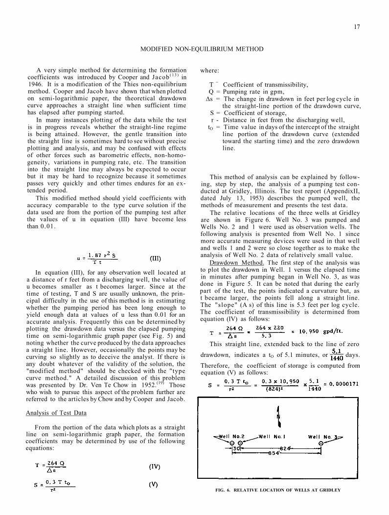
This method of analysis can be explained by follow­ing, step by step, the analysis of a pumping test con­ducted at Gridley, Illinois. The test report (AppendixII, dated July 13, 1953) describes the pumped well, the methods of measurement and presents the test data.

The relative locations of the three wells at Gridley are shown in Figure 6. Well No. 3 was pumped and Wells No. 2 and 1 were used as observation wells. The following analysis is presented from Well No. 1 since more accurate measuring devices were used in that well and wells 1 and 2 were so close together as to make the analysis of Well No. 2 data of relatively small value.

Drawdown Method. The first step of the analysis was to plot the drawdown in Well. 1 versus the elapsed time in minutes after pumping began in Well No. 3, as was done in Figure 5. It can be noted that during the early part of the test, the points indicated a curvature but, as t became larger, the points fell along a straight line. The "slope" (A s) of this line is 5.3 feet per log cycle. The coefficient of transmissibility is determined from equation (IV) as follows:

This straight line, extended back to the line of zero

drawdown, indicates a tO of 5.1 minutes, or days.

Therefore, the coefficient of storage is computed from equation (V) as follows:

FIG. 6. RELATIVE LOCATION OF WELLS AT GRIDLEY

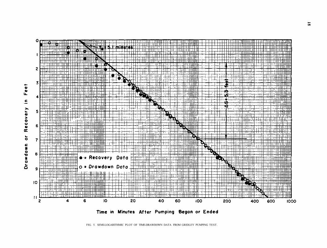
FIG. 5. SEMI-LOGARITHMIC PLOT OF TIME-DRAWDOWN DATA FROM GRIDLEY PUMPING TEST.

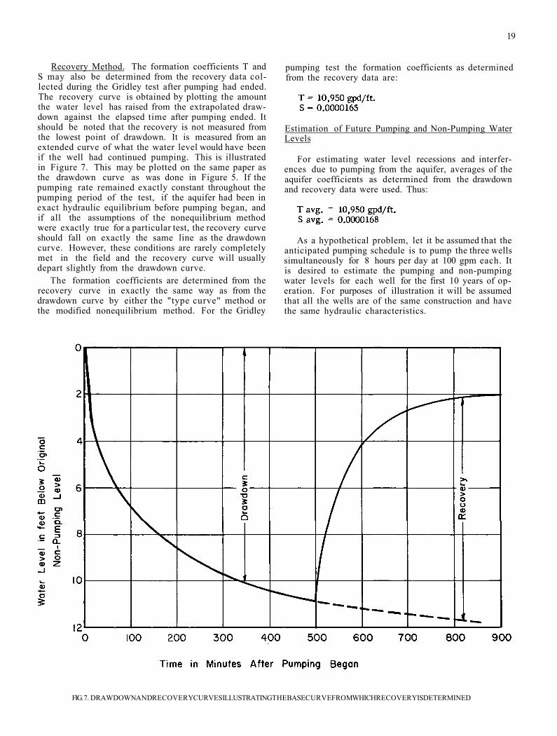
Recovery Method. The formation coefficients T and S may also be determined from the recovery data col­lected during the Gridley test after pumping had ended. The recovery curve is obtained by plotting the amount the water level has raised from the extrapolated draw­down against the elapsed time after pumping ended. It should be noted that the recovery is not measured from the lowest point of drawdown. It is measured from an extended curve of what the water level would have been if the well had continued pumping. This is illustrated in Figure 7. This may be plotted on the same paper as the drawdown curve as was done in Figure 5. If the pumping rate remained exactly constant throughout the pumping period of the test, if the aquifer had been in exact hydraulic equilibrium before pumping began, and if all the assumptions of the nonequilibrium method were exactly true for a particular test, the recovery curve should fall on exactly the same line as the drawdown curve. However, these conditions are rarely completely met in the field and the recovery curve will usually depart slightly from the drawdown curve.

The formation coefficients are determined from the recovery curve in exactly the same way as from the drawdown curve by either the "type curve" method or the modified nonequilibrium method. For the Gridley

19

pumping test the formation coefficients as determined from the recovery data are:

Estimation of Future Pumping and Non-Pumping Water Levels

For estimating water level recessions and interfer­ences due to pumping from the aquifer, averages of the aquifer coefficients as determined from the drawdown and recovery data were used. Thus:

As a hypothetical problem, let it be assumed that the anticipated pumping schedule is to pump the three wells simultaneously for 8 hours per day at 100 gpm each. It is desired to estimate the pumping and non-pumping water levels for each well for the first 10 years of op­eration. For purposes of illustration it will be assumed that all the wells are of the same construction and have the same hydraulic characteristics.

FIG. 7. DRAWDOWN AND RECOVERY CURVES ILLUSTRATING THE BASE CURVE FROM WHICH RECOVERY IS DETERMINED

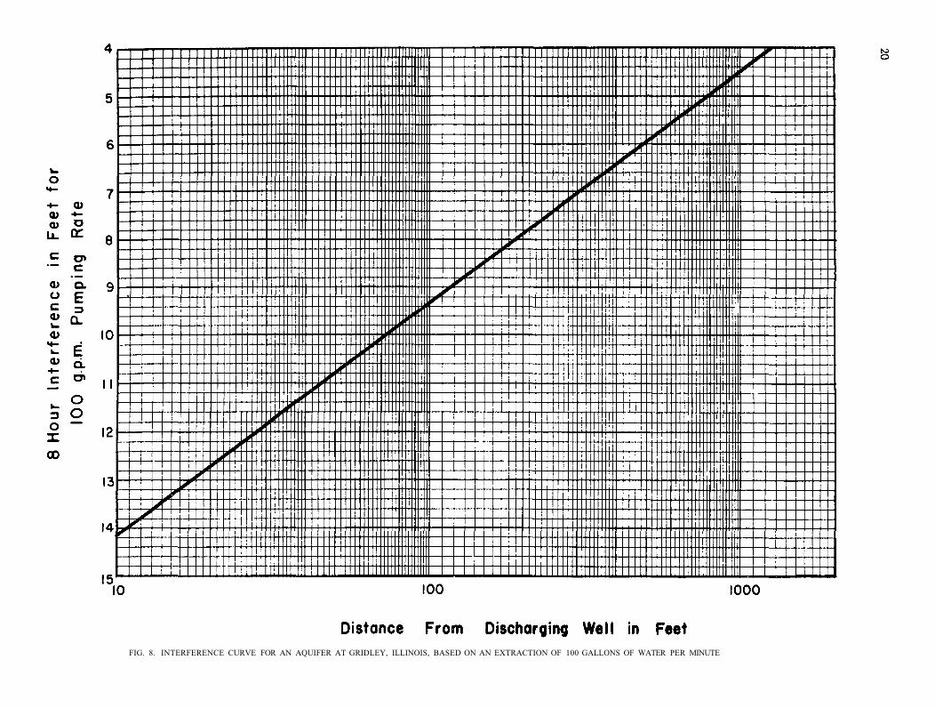
FIG. 8. INTERFERENCE CURVE FOR AN AQUIFER AT GRIDLEY, ILLINOIS, BASED ON AN EXTRACTION OF 100 GALLONS OF WATER PER MINUTE

In order to estimate the pumping levels in the wells, three things must be considered.

1.) The drawdown in each well caused by its own pumping.

2.) The interference in each well caused by the other wells pumping.

3.) The areal recession of the water level due to the long-term extraction of water from the aquifer.

Self-caused Drawdown. The drawdown in each well caused by its own pumping (assumed to be the same in each well) can be estimated from the drawdown in Well No. 3 during the pumping test. The 8 hour draw­down in Well No. 3 while pumping at 220 gpm was 31.5 feet. An approximate figure for the drawdown while pumping at 100 gpm can be had by multiplying

the ratio feet. In making this esti­mate of the drawdown at 100 gpm it was assumed (neg­lecting well loss) that the drawdown was proportional to the pumping rate. That is to say Sw = BQ. A better equation is Sw = BQ + CQ2 , where Sw is the drawdown in the well, Q is the pumping rate, and B and C are constants. However, in the absence of a step drawdown test the constants B and C cannot be accurately evaluated. The next best alternative is to use the equation Sw = BQ which would ordinarily give a slightly greater drawdown than the actual when adjusting from a higher pumping rate to a lower one as was done here. Conversely, it would yield a slightly smaller drawdown than would actually occur when adjusting from a lower pumping rate to a higher one. For a better understanding of the factors involved, see the section on the step-drawdown test.

Interference. In estimating the drawdown in each well caused by the pumping of the other wells, it is convenient to construct an interference curve. This is done with the use of Table I and equations (I) and (III)

21

It is desired to calculate the interference at the end of the daily 8 hour schedule in each well caused by the other wells pumping. For this case u =

where r is in feet from a discharging well. Equation (I) becomes:

An interference table is then set up as follows:

Table II Eight Hour - 100 gpm.

Interference Calculations Distance from

Discharging Well r feet

r 2 u W(u) Inter­

ference s feet

10 100

1000

100 10.000

1,000,000

8. 6× 1 0 - 7

8.6 × 1 0 - 5

8 . 6 × l 0 - 3

13 3891 8. 7840 4. 1974

13.99 9. 17 4 38

In Table II. the values of r were selected as multiples of 10 for ease of calculation. The values of u were cal­culated by equation (III). The values of W(u) were ob­tained from Table I for the corresponding values of u. The values of s were then calculated by equation (I).

The interference curve is obtained by plotting r versus s on semi-logarithmic graph paper as shown in Figure 8. For a case where u is less than 0.01, only two val­ues of s need be calculated, for the semi-logarithmic relationship is a straight line. From this interference curve a table of interferences may be compiled show­ing the interference of each well on the others and the total interference in each well (see Table HI). The total drawdown is obtained by adding the self-caused drawdown of 14.3 feet to the total interference of each well.

Table III

Interference Between Wells

Eight Hours Pumping At 100 gpm For Each Well

Interfering Well

Well No. 1 Well No. 2 Well No. 3

Well No 1 Well No . 2 Well No. 3 Interfering

Well

Well No. 1 Well No. 2 Well No. 3

Distance between wells

in feet

Inter­ference in feet

Distance between wells

in feet

Inter­ference in feet

Distance between wells

in feet

Inter­ference in feet

Interfering Well

Well No. 1 Well No. 2 Well No. 3

30 824

11.85 4.90

30

854

11.85

4.85

824 854

4.90 4.85

Total Inter­ferences in feet

Self-caused drawdown

16.75

14.30

16.70

14.30

9.75

14.30 Total draw­down in feet 31.05 31.00 24.05

22

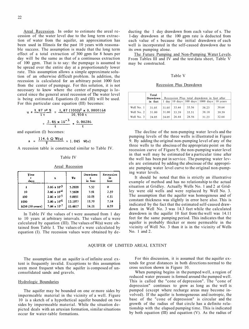
Areal Recession. In order to estimate the areal re­cession of the water level due to the long term extrac­tion of water from the aquifer, an approximation has been used in Illinois for the past 10 years with reasona­ble success. The assumption is made that the long term effect of a total extraction of 300 gpm for 8 hours per day will be the same as that of a continuous extraction of 100 gpm. That is to say: the pumpage is assumed to be spread over the entire day at a proportionately lower rate. This assumption allows a simple approximate solu­tion of an otherwise difficult problem. In addition, the recession is calculated for an arbitrary point 1000 feet from the center of pumpage. For this solution, it is not necessary to know where the center of pumpage is lo­cated since the general areal recession of The water level is being estimated. Equations (I) and (III) will be used. For this particular case equation (III) becomes:

and equation (I) becomes:

A recession table is constructed similar to Table IV.

Table IV

Areal Recession

In Table IV the values of t were assumed from 1 day to 10 years at arbitrary intervals. The values of u were calculated by equation (III). The values of W(u) were ob­tained from Table I. The values of s were calculated by equation (I). The recession values were obtained by de­

ducting the 1 day drawdown from each value of s. The 1-day drawdown at the 100 gpm rate is deducted from each value of s because the initial drawdown of each well is incorporated in the self-caused drawdown due to its own pumping alone.

The Future Pumping and Non-Pumping Water Levels. From Tables III and IV and the test data sheet, Table V may be constructed.

Table V

Recession Plus Drawdown

Total Drawdown

in feet Recession Plus total drawdown in feet after

Total Drawdown

in feet 1 day 10 days 100 days 1000 days 10 years

Well No. 1 31.05 31.05 33.44 35.56 38.23 39.64 Well No. 2 31.00 31.00 33.39 35.51 38.18 39.59 Well No. 3 24.05 24.05 26.44 28.56 31.23 32.64

The decline of the non-pumping water levels and the pumping levels of the three wells is illustrated in Figure 9. By adding the original non-pumping level of any of the three wells to the abscissa of the appropriate point on the recession curve of Figure 9, the non-pumping water level in that well may be estimated for a particular time after the well has been put in service. The pumping water lev­els are estimated by adding the abscissae of the appropri­ate pumping water level curve to the original non-pump-ing water levels.

It should be noted that this is strictly an illustrative example of method and has no relationship to the actual situation at Gridley. Actually Wells No. 1 and 2 at Grid-ley were old wells and were replaced by Well No. 3. The assumption that the aquifer was homogenous and of constant thickness was slightly in error here also. This is indicated by the fact that the estimated self-caused draw­down in Well No. 3 was 14.3 feet while the calculated drawdown in the aquifer 10 feet from the well was 14.11 feet for the same pumping period. This indicates that the aquifer is probably thicker or more permeable in the vicinity of Well No. 3 than it is in the vicinity of Wells No. 1 and 2.

AQUIFER OF LIMITED AREAL EXTENT

The assumption that an aquifer is of infinite areal ex­tent is frequently invalid. Exceptions to this assumption seem most frequent when the aquifer is composed of un­consolidated sands and gravels.

Hydrologic Boundaries

The aquifer may be bounded on one or more sides by impermeable material in the vicinity of a well. Figure 10 is a sketch of a hypothetical aquifer bounded on two sides by impermeable material. While the situation de­picted deals with an artesian formation, similar situations occur for water-table formations.

For this discussion, it is assumed that the aquifer ex­tends for great distances in both directions normal to the cross section shown in Figure 10.

When pumping begins in the pumped well, a region of reduced water pressure is formed around the pumped well. This is called the "cone of depression". The "cone of depression" continues to grow as long as the well is pumped (except where recharge areas may become in­volved). If the aquifer is homogeneous and isotropic, the base of the "cone of depression" is circular and the growth of the radius of that circle has a definite rela­tionship with the elapsed pumping time. This is indicated by both equation (III) and equation (V). As the radius of

FIG. 9. ESTIMATED FUTURE WATER LEVELS IN GRIDLEY ILLINOIS MUNICIPAL WELLS.

24

FIG. 10. HYPOTHETICAL CROSS-SECTION SHOWING AN AQUIFER OF LIMITED AREAL EXTENT

the base of the "cone of depression" grows it passes the observation well and the water level in the observation well begins to lower. As the cone continues to grow, it eventually touches the impermeable boundary to the right of the pumped well. It can no longer grow in that direc­tion.

The behavior of the cone of depression, where there is only one boundary, is conveniently described in terms of the interference of an imaginary well, called an "image well". The image well is considered to be lo­cated twice as far from the pumped well as the imper­meable boundary. A line between the pumped well and the image well is at right-angles to the impermeable boundary. Figure 11 is a cross section of the idealized aquifer (including image well) that would be imagined, for purposes of analysis, to replace the right-hand portion of the situation shown in Figure 10.

The image well is assumed to be pumped at exactly the same rate as the pumped well. Since the formation is homogeneous and isotropic, the cone of depression for the image well touches the boundary at the same time that the acutal cone touches it. From this point on, as pump­ing continues, the effect on the shape of the cone of de­pression of the pumped well is exactly the same as that

of a real well located where the image well is postulated. The cone of depression of the pumped well is conceived of as extending beyond the boundary. Simultaneously, the imaginary cone of depression is conceived to extend beyond the boundary toward the pumped well, thus dou­bling the values of s in the area where the real and im­aginary cones of depression overlap.

As this process continues, the actual cone of depres­sion, modified by the effect of the image well, proceeds toward the left from the boundary toward the pumped well. In the particular situation described, the modified cone reaches first the observation well, and next the pumped well. At the time when the modified cone reaches the observation well, the slope of the recession curve plotted on semi-logarithmic paper doubles. Simi­larly when the modified cone of depression reaches the pumped well, the slope of its "recession curve" doubles.

Figure 11 shows this situation for the right-hand bound­ary in section. For purposes of simplicity, the state of the modified cone prior to its arrival at the observation well is depicted. As the pumping continues, the entire cone of depression shifts downward, and distances " a " and " b " increase.

To complete the analysis of the situation shown in Figure 10, it is assumed the two boundaries are replaced by two image wells which start pumping at the same time and at the same rate of production as the pumped well. The effect of the second image well is similar to that of the first. Figure 12 depicts the type of drawdown curve that would occur in the observation well shown in Figure 10, when two boundaries are present.

Under boundary conditions, the water level in the ob­servation well would remain unchanged for a period of

FIG. 11. IMAGINARY AQUIFER ASSUMED TO REPLACE HALF OF THE AQUIFER IN FIGURE 10 FOR THE PURPOSES OF ANALYSIS

25

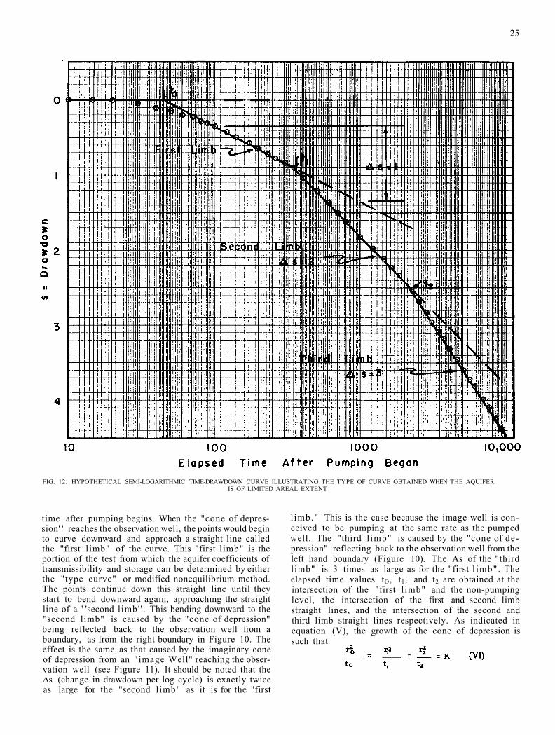
FIG. 12. HYPOTHETICAL SEMI-LOGARITHMIC TIME-DRAWDOWN CURVE ILLUSTRATING THE TYPE OF CURVE OBTAINED WHEN THE AQUIFER IS OF LIMITED AREAL EXTENT

time after pumping begins. When the "cone of depres­sion' ' reaches the observation well, the points would begin to curve downward and approach a straight line called the "first l imb" of the curve. This "first limb" is the portion of the test from which the aquifer coefficients of transmissibility and storage can be determined by either the "type curve" or modified nonequilibrium method. The points continue down this straight line until they start to bend downward again, approaching the straight line of a ' 'second l imb' ' . This bending downward to the "second limb" is caused by the "cone of depression" being reflected back to the observation well from a boundary, as from the right boundary in Figure 10. The effect is the same as that caused by the imaginary cone of depression from an "image Well" reaching the obser­vation well (see Figure 11). It should be noted that the ∆s (change in drawdown per log cycle) is exactly twice as large for the "second l imb" as it is for the "first

l imb." This is the case because the image well is con­ceived to be pumping at the same rate as the pumped well. The "third l imb" is caused by the "cone of de­pression" reflecting back to the observation well from the left hand boundary (Figure 10). The As of the "third l imb" is 3 times as large as for the "first l imb". The elapsed time values tO, t1, and t2 are obtained at the intersection of the "first l imb" and the non-pumping level, the intersection of the first and second limb straight lines, and the intersection of the second and third limb straight lines respectively. As indicated in equation (V), the growth of the cone of depression is such that

26

Where:

rO = Distance from pumped well to observation well

r1 = Distance from image well (1) to observation well

r2 = Distance from image well (2) to observation well

K =A constant

Since rO, tO, t1, and t2 of equation (VI) can be de­termined by measurements in the field and from exam­ination of Figure 12, it is possible to solve for the dis­tances from the observation well to image wells (1) and (2).

If more than one observation well is available, equa­tion (VI) may be applied to each observation well and the locations of the "image wells" may be more accur­ately determined as to direction. Only rarely are the water level data of the pumped well sufficiently reliable for equation (VI) to be applied to the pumped well. Slight variations in pumping rate usually cause the water level in the pumped well to fluctuate to such an extent that the various "limbs" of a curve of the type in Figure 12 can not be accurately determined. Naturally, if there is no observation well, equation (VI) is not applicable to the pumped well since r is missing. Theoretically it

takes three or more wells to which equation (VI) may be applied to locate definitely the positions of the "image wells". If only two wells are available to which equation (VI) may be applied, the position of each "image well" may be narrowed down to one of two possible locations.

The impermeable boundaries are known to be half way between the "image wells" and the pumped well.

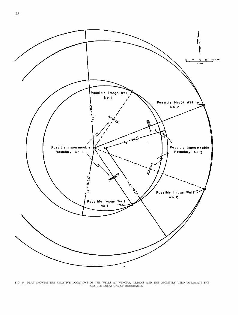
Example of Analysis. The method of locating first the "image wells" and then the boundaries will be illus­trated by a step-by-step analysis of data from a pumping test conducted at Wenona, Illinois. A copy of the pumping test report dated October 14,1947 is included in Appendix II.

The pumping test at Wenona, Illinois was one of the rare cases in which equation (VI) could be applied to the pumped well. Forthatreason it was selected as an exam­ple here since it illustrates the application of equation (VI) to an observation well and to a pumped well.

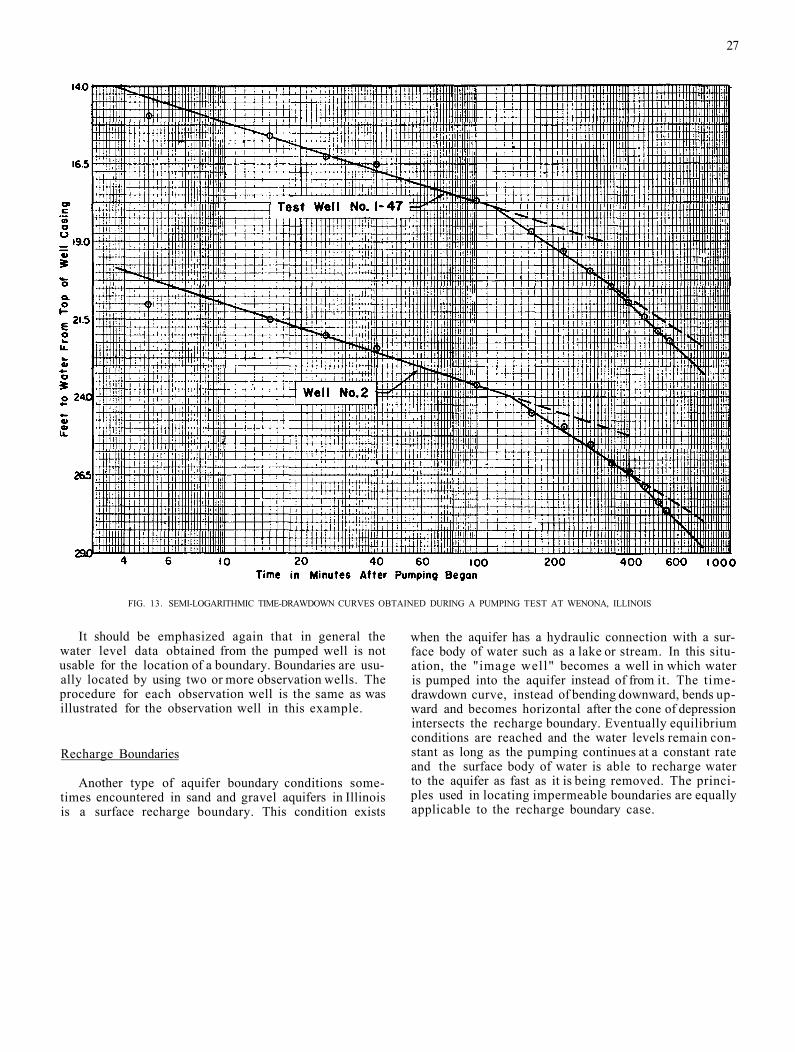
The first step of the analysis is to plot the water level data from the observation well (test well No. 1-47) and the pumped well (well No. 2) on semi-logarithmic graph paper as shown in Figure 13. The three limbs are fitted to the plotted points of each well so that the A s (draw­down per log cycle) values are proportioned to a 1:2:3 ratio. For both wells the A s values are as follows:

Limb ∆s

1st 2.65 ft/Log. cycle 2nd 5.30 ft/Log. cycle 3rd 7.95 ft/Log. cycle

For the observation well, tO = 3.7 minutes, t1 =115

minutes, and t2 = 340 minutes. The distance from the

center of the pumped well to the center of the observa­tion well is 17.17 feet. By equation (VI),

In the above calculations r01. is the distance from the observation well to the first "image well" and R02 is the

distance from the observation well to the second "image well".

The same value of K is used for the pumped well as for the observation well.

Equation (VI) applied to the pumped well yields the following results:

The value of r is the distance between the pumped

well and the first "image well" and rp2 is the distance

between the pumped well and the second "image well" . The next step of the analysis is to plot the possible

locations of the "image wells". This was done in Figure 14 by the following method. A suitable scale was chosen and the relative locations of the pumped well and the ob­servation well were plotted on a plan. A circle of radius. r01 having its center at the observation well was drawn.

A circle radius of r . with its center at the pumped well

was drawn. These two circles should intersect at two points which are the two possible locations of "image well" No. 1. The two possible locations of the first im­permeable boundary are half way between these' ' image well" locations and the pumped well. This gives two possible locations for the first impermeable boundary. Unless additional information is available, it is notpos-sible to be sure which of these locations is occupied by the first impermeable boundary. If another observation well were available, the circle drawn from itshould in­tersect the circles from this observation well and the pumped well at or near one of the two points of intersec­tion shown on Figure 14. This common point of intersec­tion would then be the effective location of the first "image well". Frequently some additional knowledge of the geology of the area will aid in the selection of the correct boundary location.

The probable locations of the second "image well" and consequently the second impermeable boundary are found in exactly the same way as for the first image well, except that r02 and rp 2 are used.

27

FIG. 13. SEMI-LOGARITHMIC TIME-DRAWDOWN CURVES OBTAINED DURING A PUMPING TEST AT WENONA, ILLINOIS

It should be emphasized again that in general the water level data obtained from the pumped well is not usable for the location of a boundary. Boundaries are usu­ally located by using two or more observation wells. The procedure for each observation well is the same as was illustrated for the observation well in this example.

Recharge Boundaries

Another type of aquifer boundary conditions some­times encountered in sand and gravel aquifers in Illinois is a surface recharge boundary. This condition exists

when the aquifer has a hydraulic connection with a sur­face body of water such as a lake or stream. In this situ­ation, the "image well" becomes a well in which water is pumped into the aquifer instead of from it. The time-drawdown curve, instead of bending downward, bends up­ward and becomes horizontal after the cone of depression intersects the recharge boundary. Eventually equilibrium conditions are reached and the water levels remain con­stant as long as the pumping continues at a constant rate and the surface body of water is able to recharge water to the aquifer as fast as it is being removed. The princi­ples used in locating impermeable boundaries are equally applicable to the recharge boundary case.

28

FIG. 14. PLAT SHOWING THE RELATIVE LOCATIONS OF THE WELLS AT WENONA, ILLINOIS AND THE GEOMETRY USED TO LOCATE THE POSSIBLE LOCATIONS OF BOUNDARIES

29

STEP DRAWDOWN TESTS

General Discussion

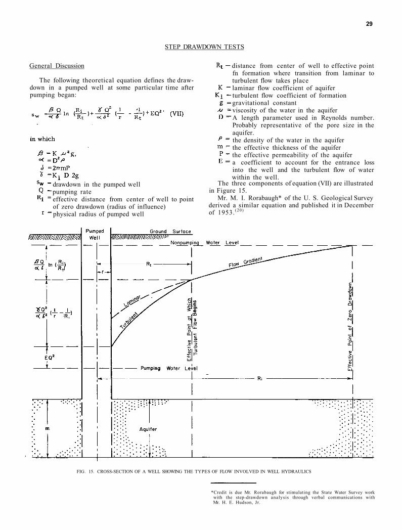
The following theoretical equation defines the draw­down in a pumped well at some particular time after pumping began:

drawdown in the pumped well pumping rate effective distance from center of well to point of zero drawdown (radius of influence) physical radius of pumped well

distance from center of well to effective point fn formation where transition from laminar to turbulent flow takes place laminar flow coefficient of aquifer turbulent flow coefficient of formation gravitational constant viscosity of the water in the aquifer A length parameter used in Reynolds number. Probably representative of the pore size in the aquifer. the density of the water in the aquifer the effective thickness of the aquifer the effective permeability of the aquifer a coefficient to account for the entrance loss into the well and the turbulent flow of water within the well.

The three components of equation (VII) are illustrated in Figure 15.

Mr. M. I. Rorabaugh* of the U. S. Geological Survey derived a similar equation and published it in December of 1953. (20 )

FIG. 15. CROSS-SECTION OF A WELL SHOWING THE TYPES OF FLOW INVOLVED IN WELL HYDRAULICS

*Credit is due Mr. Rorabaugh for stimulating the State Water Survey work with the step-drawdown analysis through verbal communications with Mr. H. E. Hudson, Jr.

30

Because of the many factors in equation (VII) that cannot be measured, it is not practical for engineering use in its basic form. However, the equation is an aid to understanding the various factors and how they affect the drawdown. Further, if the assumptions made for the non-equilibrium method are valid for a particular case, equation (VII) can be simplified and used conveniently by making one additional assumption. This assumption is that equation (VII), rearranged as follows:

and further simplified to:

yields

and

As a simplification, CQ2 may be taken to represent the well loss. This assumption is not entirely valid be­cause Rt will increase as Q is increased. This actually makes B and C variables in equation (VIII). However, as B increases, C decreases and if B and C are assumed to be constants, the error in one component of equation (VIII) tends to compensate for the error in the other. Although, the error in one component will not entirely correct the error in the other component, equation (VIII) can be used to obtained fairly reliable values of draw­down over the range of pumping rates generally needed for a particular well.

If it is desired to extrapolate the values of drawdown over a great range of values of pumping rate, the reader is referred to Mr. Rorabaugh'spaper.(20) Mr. Rorabaugh attempts to compensate for the variation in Rt by using the following equation:

in which n is greater than 2. In the opinion of the authors, Mr. Rorabaugh presents the most exact method presently available when a larger range of pumping rates is en­countered but the solution is complicated by the evalua­tion of the three terms B, C, and n. In practice, equation (VIII) has been found to be very useful. More research needs to be done with this type of analysis in order to evaluate accurately the numerous factors involved.

If equation (VIII) is adequate for the range of pumping rates involved, the analysis proceeds as in the following example.

Example of Analysis

The example chosen to illustrate the approximate analysis of the step-drawdown test is a pumping test of

an irrigation well located in the Mississippi River low­lands near Granite City, Illinois.

The pumping test report of the Thomason Irrigation Well No. 1 dated May 21, 1954 gives a brief description of the well (see Appendix II). The well was pumped at three rates, 1000, 1280, and 1400 gallons per minute. The lowest pumping rate was maintained for the longest period in order to determine the recession curve for that pumping rate. The recession curves at the higher pump­ing rates can be estimated from this first recession curve. In the analysis of these data, time was taken into account in a way that would eliminate effects of progressive recession on the data. Values of sw were determined after one hour of pumping at each new rate.

Therefore the estimated slope at 1280 gpm was about 0.269 feet per log cycle and the slope at 1400 gpm was about 0.294 feet per log cycle. These slopes were used to extrapolate each step of the test beyond the period of pumping of each step as shown by the dashed lines in Figure 16. These extrapolations were used to obtain the incremental drawdown caused by a change in pump­ing rate. Before the test was started, the pumping rate was zero and the water level in the well stood at a constant level. When the pumping test began, the pump­ing rate immediately increased from zero to 1000 gpm. After one hour of pumping the incremental drawdown was 5.43 feet. The pumping rate in this case was con­tinued at 1000 gpm for a total of 100 minutes when the pumping rate was increased to 1280 gpm. One hour after the pumping rate was increased the incremental draw­down caused by the 280 gpm increase was 1.59 feet. The same procedure was followed for each step of the test.

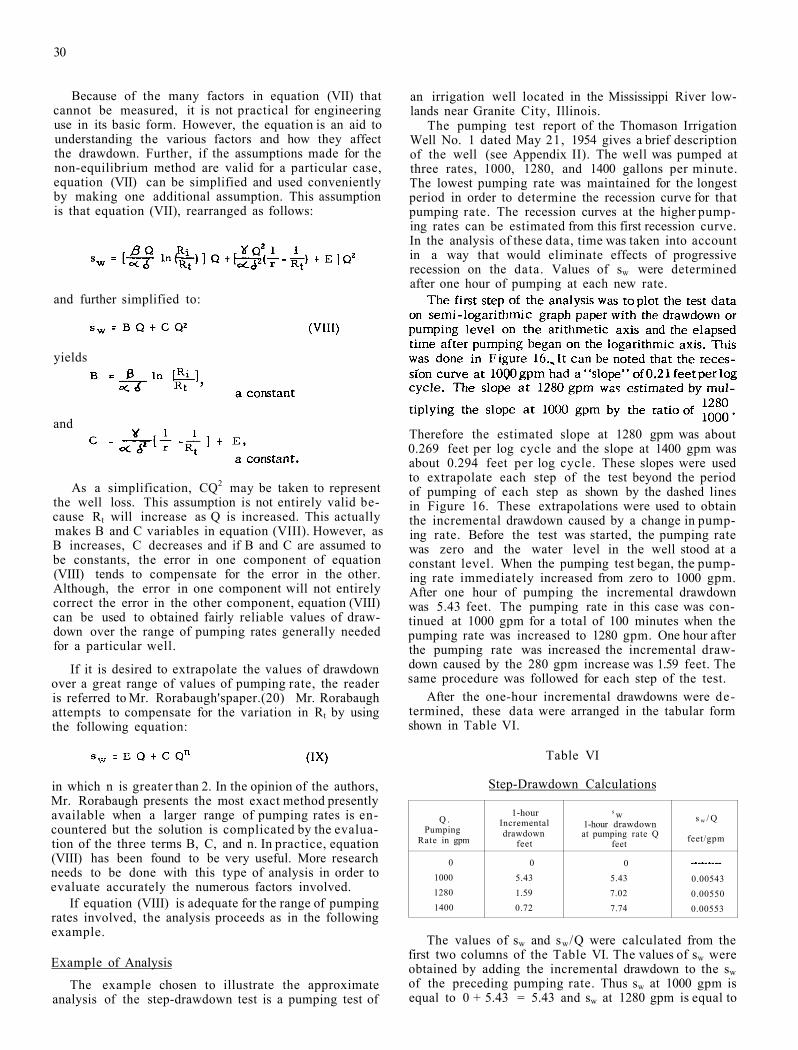
After the one-hour incremental drawdowns were de­termined, these data were arranged in the tabular form shown in Table VI.

Table VI

Step-Drawdown Calculations

Q . Pumping

Rate in gpm

1-hour Incremental drawdown

feet

s w 1-hour drawdown at pumping rate Q

feet

s w / Q

feet/gpm

0 1000 1280 1400

0 5.43 1.59 0.72

0 5.43 7.02 7.74

0.00543 0.00550 0.00553

The values of sw and sw /Q were calculated from the first two columns of the Table VI. The values of sw were obtained by adding the incremental drawdown to the sw of the preceding pumping rate. Thus sw at 1000 gpm is equal to 0 + 5.43 = 5.43 and sw at 1280 gpm is equal to

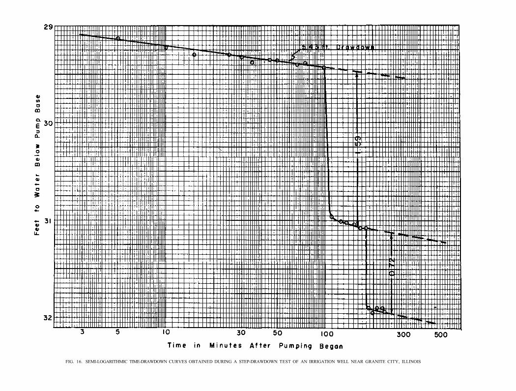
FIG. 16. SEMI-LOGARITHMIC TIME-DRAWDOWN CURVES OBTAINED DURING A STEP-DRAWDOWN TEST OF AN IRRIGATION WELL NEAR GRANITE CITY, ILLINOIS

32

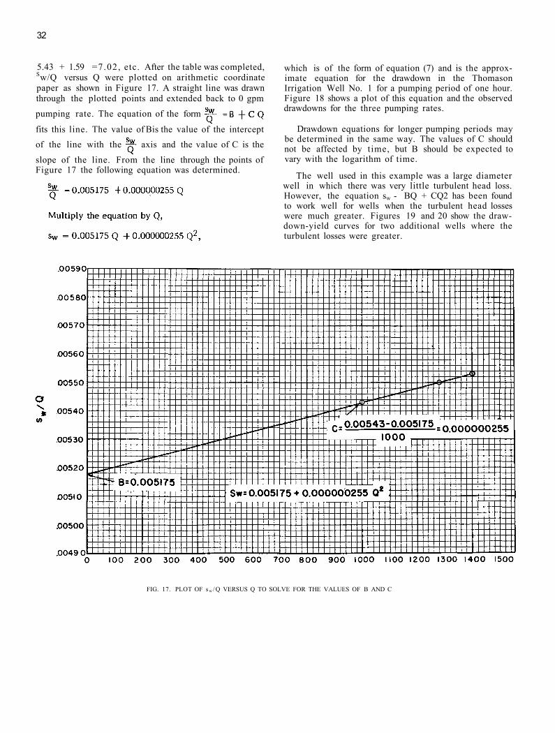
5.43 + 1.59 =7.02, etc. After the table was completed, Sw/Q versus Q were plotted on arithmetic coordinate paper as shown in Figure 17. A straight line was drawn through the plotted points and extended back to 0 gpm

pumping rate. The equation of the form

fits this line. The value of Bis the value of the intercept of the line with the axis and the value of C is the

slope of the line. From the line through the points of Figure 17 the following equation was determined.

which is of the form of equation (7) and is the approx­imate equation for the drawdown in the Thomason Irrigation Well No. 1 for a pumping period of one hour. Figure 18 shows a plot of this equation and the observed drawdowns for the three pumping rates.

Drawdown equations for longer pumping periods may be determined in the same way. The values of C should not be affected by time, but B should be expected to vary with the logarithm of time.

The well used in this example was a large diameter well in which there was very little turbulent head loss. However, the equation sw - BQ + CQ2 has been found to work well for wells when the turbulent head losses were much greater. Figures 19 and 20 show the draw­down-yield curves for two additional wells where the turbulent losses were greater.

FIG. 17. PLOT OF s w / Q VERSUS Q TO SOLVE FOR THE VALUES OF B AND C

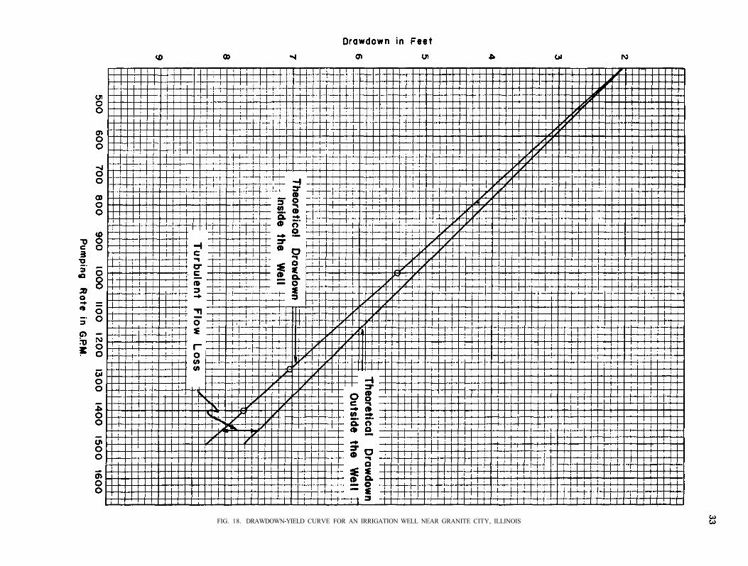
FIG. 18. DRAWDOWN-YIELD CURVE FOR AN IRRIGATION WELL NEAR GRANITE CITY, ILLINOIS

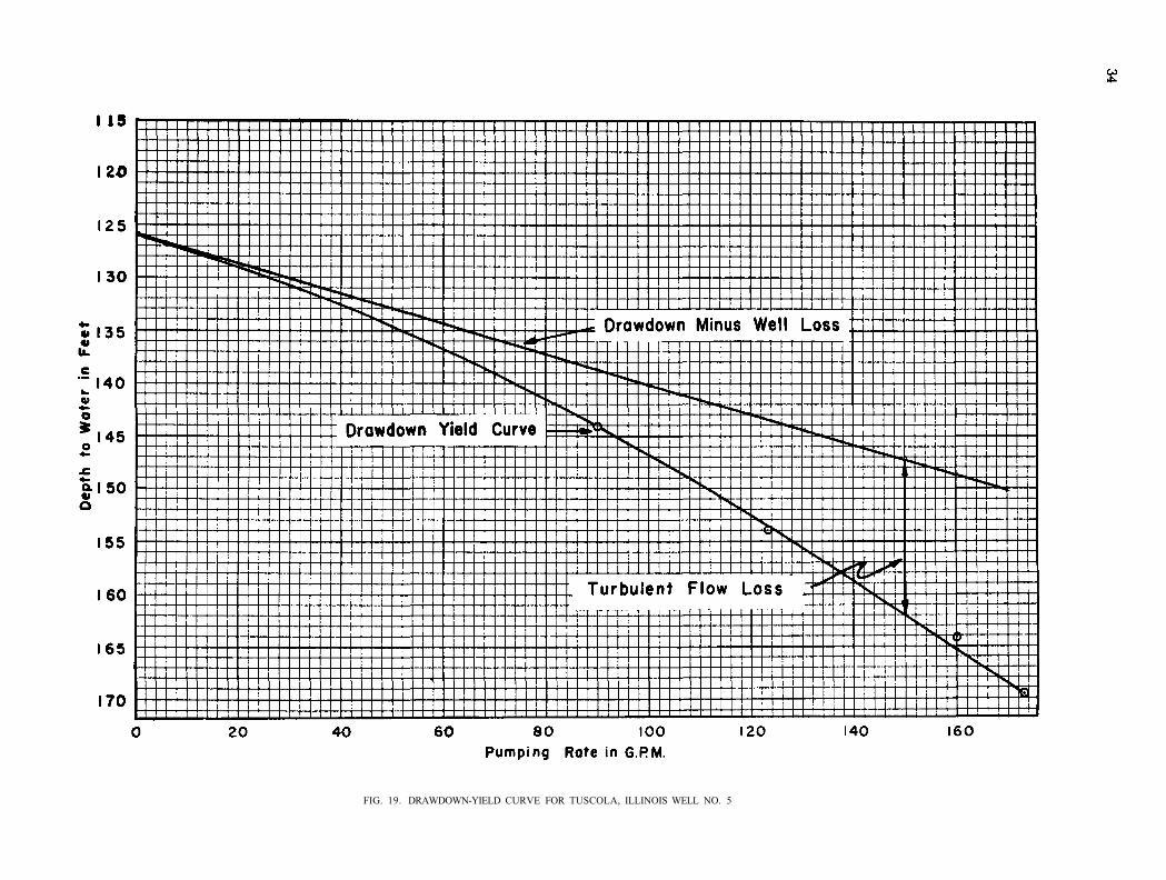
FIG. 19. DRAWDOWN-YIELD CURVE FOR TUSCOLA, ILLINOIS WELL NO. 5

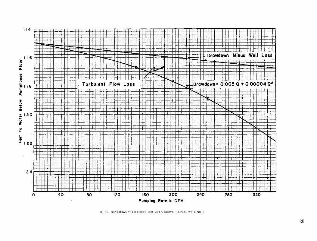
FIG. 20. DRAWDOWN-YIELD CURVE FOR VILLA GROVE, ILLINOIS WELL NO. 2

36

COMPLICATING FACTORS

The cases given in the foregoing material were chosen because they were relatively clean-cut and simple, and because they clearly illustrated some of the less-well known basic methods with which groundwater problems are attacked. In many instances, the data from pump­ing tests do not lend themselves to precise analysis by the above methods because of interference by factors not encountered in these cases.

The accurate determination of the non-pumping water level is imperative for the methods of analysis described in this report. Whenever possible, all nearby pumping from the aquifer should be discontinued for a period prior to and during the pumping test. The period of shutdown should be of sufficient duration to allow the water level (or pressure) in the aquifer to closely ap­proach an equilibrium condition. The time required is usually determined by periodically measuring the water levels in various observation wells after the shutdown. When the water levels in all of the wells have assumed a constant level, the pumping test may be started.

When it is impossible to discontinue all pumping from the aquifer, the pumping of all wells should be controlled and should be kept constant for the period preceding and during the pumping test. The trend of the change in water levels must be determined prior to the start of the pumping test. In this case, all drawdown data must then be determined from the water-level trend curve rather than from single measured non-pump­ing levels. The degree of control over all possible interfering pumping from the aquifer has a direct bear­ing on the accuracy of the pumping test results.

The section on boundary conditions mentioned the characteristic shape of the drawdown-log time curve that would be expected under recharge conditions. A similar shape may be produced under some instances by transition of the situation in a formation from an artesian condition to a partial or virtually complete water-table condition. Such a change produces a large increase in the coefficient of storage, and actual dewatering of the formation commences sometime after the beginning of the test. A decline in pumping rate may produce a similar curve. A number of cases have been experienced in which water discharged from the well was not effec­tively conducted away from the vicinity of the well, and seeped back into the water-bearing formation, thus producing actual recharge which would not take place under normal operating conditions.

In artesian aquifers, changes in barometric pressure may cause the water level to change. These effects may cause variances in water level as great as one foot. Such variances may be identified if a precise record of variations in barometric pressure is available in the vicinity of the test. Allowance must be made for the fact that such data, obtained from recording barographs located at a distance from the point of test, may have to be adjusted to correct for time lag between the point of barometric pressure measurements and the place of the well test. In addition, since the variation in water level in a well depends on the barometric efficiency of the aquifer, data under non-pumping conditions will be

necessary in order to determine the barometric correc­tions to be made. Barometric efficiency may vary from zero under water table conditions to nearly 100 per cent. Similar effects of even greater magnitude occur in wells near streams as a result of stream level fluctuations.(25)

In the examples discussed in this report, the data in­dicated that the assumption of an isotropic, homogenous formation was valid. In a number of instances, data un­affected by other complicating factors gave reason to believe that this assumption was not valid. In some instances the data indicated variances in coefficient of storage as the cone of depression grew. In other cases there were indications that the transmissibility of the formation varied considerably from the vicinity of the well to more remote areas. Where these variations are major, it is clear that a large number of observation wells and a considerable amount of additional test drill­ing may be necessary to accurately evaluate the under­ground conditions. The application of non-equilibrium methods does not become useless under these conditions: it may be an aid in determining what the actual under­ground conditions are and may clearly point out needs for further exploration.

In some instances, alluvial and glacial deposits are found to be highly lenticular, and sometimes have hydrologic interconnections of varying capabilities. In these instances, observation wells may yield misleading or seemingly contradictory results. Cases have also been encountered in which wells have yielded water simul­taneously from more than one formation. In these cases, observation wells in any single formation have given non-representative results. Other instances have been encountered in which observation wells have been found to be in a formation completely separate from that con­nected to the pumped well.

Misleading results are also obtained from observation wells that are not constructed to be fully open into the pumped formation. An observation well must have permeable connection into the water-yielding formation. The test for this is to pour a quantity of water into the observation well sufficient to raise its level by a readily measureable amount. Timed readings of the water-level change are then taken on the observation well to see how rapidly the water level returns to its original elevation.

For work with the non-equilibrium method, a con­stant pumping rate is nearly imperative throughout a major part of each pumping test. If underground con­ditions are particularly complex or obscure, an extended period of pumping at a constant rate is important. This extended time of pumping at a constant rate may need to be as long as several weeks, although ordinarily, two or three days will suffice, and in cases known to be un­complicated, a few hours may be sufficient.

Gradual changes in pumping rate may have ruinous effect upon drawdown data, and are more to be guarded against than abrupt controlled changes, which may be desirable for step-drawdown analysis of the performance of the well. These controlled changes, however, are

generally of little value in evaluating water-yielding formation characteristics.

Misleading results may also be obtained from partial penetration conditions, under which either the pumped well or the observation well may not be constructed through the full thickness of the formation. Since water­bearing formations are frequently stratified, and vertical permeability is generally considerably smaller than hor­izontal permeability, partial penetration data may give unreliable results. Methods of correction for partial pen­

etration are available in the literature, but these have not always been found to be entirely satisfactory. For op­timum results, the pumped well should substantially pen­etrate the water-bearing formation and the observation wells should do likewise. If partial penetration must be present, it should be equal in observation wells and pumped wells.

Especial care must be taken in applying the non-equilibrium method to creviced or cavernous formations.

37

38

REFERENCES

1. Darcy, Henri, Les Fontaines publiques de la ville de Dijon, Paris, 1856.

2. Dupuit, Jules, Etudes theoretiques et pratiques sur le mouvement des eaux, Paris, France, 1863. Librarie des Corps Imperiax des Ponts et Chausees et des Mines.

3. Thiem, Gunter, Hydrolische Methoden, J. M. Geb-hardt, Leipzig, 1906.

4. Slichter, C. S., Theoretical Investigation of the Motion of Ground Water, U. S. Geological Survey, 19th Annual Report, 1899, Part 2, p. 360.

5. Turneaure, F. E. and Russell, H. L., Public Water Supplies, John Wiley, third edition, 1924, p. 258.

6. Israelson, O. W. Irrigation Principles and Practices, New York, John Wiley & Sons, Inc., pp. 189-211, 1950.

7. Wyckoff, R. D., Botset, H. G., and Muskat, M., Flow of Liquids through Porous Media under the Action of Gravity, Physics, Vol. 2, No. 2, pp. 90-113, 1942.

8. Wenzel, L. K., The Thiem Method for Determining Permeability of Water-bearing Materials, U. S. Geol. Survey Water-Supply Paper 679, 1937, pp. 1-57; and Methods for Determining Permeability of Water-Bearing Materials, U. S. Geol. Survey Water-Supply Paper 887, 1942, pp. 83-87.

9. Theis, C. V., The Relation between the Lowering of the Piezometric Surface and the Rate and Dura­tion of Discharge of a Well Using Ground Water Storage, Trans, A. G. U., 1935, pp. 519-524.

10. Wenzel, L. K., Methods for Determining Perme­ability of Water-Bearing Materials, U. S. Geol. Survey, Water-Supply Paper 887, 1942, p. 88.

11. Jacob, C. E., On the Flow of Water in An Elastic Artesian Aquifer, Trans. A. G. U., Part II 1940, p. 582.

12. Wenzel, L. K., and Greenlee, A. L., A Method for Determining Transmissibility and Storage Coef­ficients by Tests of Multiple Well Systems, Trans. A. G. U., Part II 1943, pp. 547-560.

13. Cooper, H. H. and Jacob, C. E. , A Generalized

Graphical Method for Evaluating Formation Con­stants and Summarizing Well-Field History, Trans. A. G. U., Vol. 27, 1946, pp. 526-534.

14. Muskat, M., The Flow of Homogeneous Fluids through Porous Media, McGraw-Hill Book Co., Inc., New York, 1937.

15. Theis, C. V., The Effect of a Well on the Flow of a Nearby Stream, Trans. A. G. U., Part III, 1941, pp. 734-737.

16. Ferris, J. G., Ground-Water Hydraulics as a Geo­physical Aid, Michigan Dept. of Conservation, Tech­nical Report No. 1, Lansing, Michigan, March 1948.

17. Meinzer, Oscar E., Physics of the Earth-IX-Hydrol-ogy. McGraw-Hill Book Co., New York and London, 1942.

18. Jacob, C. E., Drawdown Test to Determine Effec­tive Radius of Artesian Well. Proc. A. S. C. E., Vol. 72, No. 5 (May, 1946), pp. 629-646.

19. Chow, V. T., On the Determination of Transmis­sibility and Storage Coefficients from Pumping Test Data. Trans. A. G. U., Vol 33, No. 3 (June, 1952), pp. 397-404.

20. Rorabaugh, M. I., Graphical and Theoretical Analy­sis of Step-Drawdown Test of Artesian Well. Proc. ASCE, Separate No. 362, Vol. 79 (December, 1953).

21. Wisler, C. O. and Brater, E. F . , Hydrology. Chapter VII, Groundwater by Ferris, John G., John Wiley & Sons, Inc., New York. (1949).

22. Jacob, C. E.f On the Flow of Water in an Elastic Artesian Aquifer. Transactions, Am. Geophysical Union, pp. 574-586. (1940 Part II).

23. Brown, R. H. Selected Procedures for Analyzing Aquifer Test Data. Journal A.W.W. A., Vol. 45, No. 8 (August 1953), pp. 844-866.

24. Habermeyer, G. C, Public Ground-Water Supplies in Illinois, Illinois State Water Survey Bulletin No. 21, 1925.

25. Suter, Max. Apparent Changes in Water Storage During Floods at Peoria, Illinois. Trans. A. G. U., Vol. 28, No. 3 (June 1947), p. 429.

39

APPENDIX I

REPORTS OF PUMPING TESTS

41

REPORT OF WELL PRODUCTION TEST OCTOBER 9, 1952

WELL NO. 1

VILLAGE OF ARROWSMITH.McLEAN CO., ILLINOIS

By

Karl R. Klingelhofer, Assistant Engineer

Representatives of J. B. Ortman & Sons, Drilling Company, conducted a well production test on the Vil­lage of Arrowsmith Well No. 1, October 6, 1952. Rep­resentatives of the village and the Water Survey observed the test.

This well was drilled by J. B. Ortman & Sons in September 1952 at a location approximately 650 feet south and 700 feet east of the NW corner of the SW 1/4 of Sec. 15, T. 23 N., R. 5 E., McLean County, Illinois.

Well Construction Data (Well No. 1) - as reported by driller:

Depth below ground surface 228 ft.

Hole size 8 in. Casing record 223 ft. of 8 in. i.d. casing*

Screen 6 ft. of Johnson Everdur, No. 60 slot

*Casing now extends 1ft. above ground, but this is to be extended.

For test purposes the well was equipped with a shaft-driven A. O. Smith vertical-turbine pump powered by a John Deere " A " tractor. The top of the bowl section and the bottom of the suction pipe were 130 feet and 157-1/2 feet respectively below the top of the casing. Because of insufficient space between the column-pipe couplings and the well casing, it was impossible to obtain water level measurements in the pumped well. During the test, water levels were measured with the Water Survey's electric dropline in a 228 foot observa­tion well equipped with screen and located 12-1/2 feet north of Well No. 1 (pumped well). The top of the casing of the observation well extended approximately 0.3 feet above ground. Discharge from the pumped well was measured with the Water Survey's 4-inch orifice tube using orifice plate No. 25.

An attempt was made to run the test October 3 but after pumping 50 minutes the test had to be discontinued because of mechanical difficulties. The test of October 6th also had to be stopped because of mechanical dif­ficulties, however this test was considerably longer than the first one.

ARROWSMITH, ILLINOIS, SEPT. 19, 1952

Log of 8 inch well drilled 650' south, 700' east of NW comer SW quarter Sec. 15, T. 23, R. 5 E., 3rd PM

in the corporate limits of Arrowsmith, McLean County, Illinois

Thickness Depth to Base

Soil, black, some humus 5 5 Clay, brown 5 10 Clay, grey, some small rock 5 15 Clay, brown, very fine 5 20 Clay, grey 35 55 Clay, grey, some chips and gravel 10 65 Clay, grey, fine gravel 2 67 Sand, some water, s tat ic level 30' 1 68 Clay, grey, some small gravel 2 70 Clay, with scattered larger gravel 15 85 Clay, with smaller gravel 5 90 Clay, with much smaller gravel 5 95 Clay, fine 5 100 Sand 5 105

Thickness Depth of Base

Clay, gravel and wood chips 5 110 Clay, some sand, wood chips 15 125 Clay, sand and gravel 10 135 Clay, sand, gravel and some stone chips 25 160 Clay, soft sandy, bearing some water 5 165 Clay, sapdy containing much large gravel 25 190 Clay, grey, very smooth 5 195 Clay, with very fine sand 5 200 Clay, grey and brown 5 205 Clay, grey very fine 5 210 Clay, grey, medium gravel 5 215 Large gravel, imbedded in clay 5 220 Small gravel, & sand, imbedded in clay 2 222 Good water bearing gravel 6 228

Well finished at 228 feet with 6* 60 slot "Everdur" Screen

J. B. Ortman&Sons, Kokomo, Ind.

42

Test Data Production Test-10-6-52

Well No. 1 Village of Arrowsmith, McLean Co., Illinois

by Robert Sasman

Feet to Water Time t GPM 1440 r2 from top of casing Drawdown Remarks

t (observation well)

10:35 A.M. 99.45 non-pumping water level 10:37 started pumping 10:38 1 225000 103.60 4.15 10:40 3 277 75000 10:42 5 280 45000 106.80 7.35 10:45 8 250 28126 107.20 7.75 10:47 10 250 22500 10:50 13 250 17308 107.90 8.45 10:55 18 250 12500 108.50 9.05 11:02 25 250 9000 109.10 9.65 11:10 33 250 6819 109.65 10.20 11:20 43 250 5233 110.00 10.55 11:30 53 250 4245 110.50 11.05 11:40 63 250 3571 110.80 11.35 water sample no. 1, temp. 54° F 11:50 73 250 3082 111.10 11.65 12:00 Noon 83 250 2710 111.35 11.90 12:30 113 250 1991 112.00 12.55

1:07 150 250 1500 112.55 13.10 1:30 173 250 1300 112.90 13.45 2:03 206 250 1093 113.25 13.80 2:30 233 250 966 113.40 13.95 3:00 263 250 856 113.85 14.40 3:15 278 249 810 114.00 14.55 water sample no. 2, temp. 54° F 3:23 286 787 stopped pumping 3:24 287 784 110.10 10.65 recovery 3:26 289 779 105.30 5.85 3:28 291 774 107.40 7.59 3:29 292 771 107.00 7.55 3:31 294 766 106.55 7.10 3:34 297 758 106.15 6.70 3:37 300 751 105.65 6.20 3:42 305 738 105.20 5.75 3:47 310 726 104.85 5.40 3:52 315 715 104.55 5.10 4:00 323 697 104.15 4.70 4:16 339 664 103.60 4.15 end of test

Test Data Production Test-10-3-52

Well No. 1 Village of Arrowsmith, McLean Co., Illinois

by Karl R. Klingelhofer

Feet to Water Feet to Water Time G.P.M. from top of casing Remarks Time G.P.M. from top of casing Remarks

(observation well) (observation well)

9:57 A.M. 99.37 non-pumping water level 11:01 started pumping 9:59 started pumping 11:10 stopped pumping — broken

10:00 230 universal joint 10:02 105.04 10:10 230 107.22 11:11 104.05 recovery 10:15 240 11:13 103.72 10:19 108.75 11:15 103.28 10:29 250 109.52 11:20 102.60 10:39 255 110.28 11:29 101.95 10:42 245 decreased rate 11:42 101.35 10:49 245 110.41 12:30 P.M. 100.58 10:53 stopped pumping to

universal joint grease 12:52

2:00 100.41 100.12

10:59 103.70 3:19 99.94 end of test

43

July 13, 1953

REPORT ON WELL PRODUCTION TEST

WELL NO. 3

VILLAGE OF GRIDLEY

McLEAN COUNTY, ILLINOIS

BY

Karl R. Klingelhofer, Assistant Engineer

Representatives of Layne Western Company, Water Supply Contractors, conducted a well production test on July 2, 1953 on the new village well (well No. 3) at Gridley, McLean County, Illinois. Representatives of the village; L. A. Miller & Assoc, consulting Engineers; and the State Water Survey observed the test.

This well was drilled by the Layne Western Co. in June of 1953 by the reverse rotary method. Well No. 3 is located approximately 824 feet east of Well No. 1, or approximately 3304 feet east and 840 feet north of the southwest comer of Section 4, T. 26 N., R. 3E. , McLean County, Illinois. Well No. 2 is located 30 feet west of Well No. 1.

Well construction data as reported by the driller is as follows:

Total depth 286 feet below the ground

Hole size 34 inch entire depth

Casing record 274 feet 7 inches of 10 inch pipe extending 3 feet above natural ground level.

Screen 15 feet of 10 inch Layne shutter stainless steel screen, No. 7 slot, welded to casing, ¼ inch steel plate on bottom.

Gravel Pack 25 feet of gravel pack from bottom up, 1/8 inch gravel.

The driller's log of the well is as follows: Depth in feet Material

0 - 5 Soil 5 - 60 Blue clay and boulders

60 - 69 Gravel and boulders 69 - 197 Blue clay and boulders

197 - 200 Gravel 200 - 268 Blue clay and boulders 268 - 286 Gravel, coarse, boulders 286 - 297 Shale The wells were leveled in by the engineer on the day

of the test and assuming an elevation of 200.00 feet for the top of the base plate on Well No. 3, the elevation of the top of the seam of the metal liner of Well No. 1 is 197.41 feet and the top of the concrete pedestal of Well No. 2 is 197.86 feet.

For test purposes the well was equipped with an Amer­ican Well Works vertical turbine pump which was for­merly installed in Well No. 1. This pump was powered by a direct-connected 15 H.P. electric motor with pro­visions for an emergency belt drive. The pump was re­ported to have 150 feet of 5 inch column pipe, 9 feet of 7 inch bowls, 11 stages, 10 feet of 5 inch suction pipe, and a 4 inch discharge. It is understood that this pump is to be permanently installed in Well No. 3. Discharge was measured with Layne Western's 6 inch orifice tube and a 3 inch orifice. Water levels were measured in Well No. 3 with the Water Survey's altitude gage attached to an airline extending 159 feet below the top of the well casing. Water levels were measured in Well No. 1 throughout the test by two methods; one being a Steven's float operated water level recorder system, and the other being a bubbler system which has recently been devel­oped in the Water Survey's hydraulic laboratory. Water levels in Well No. 2 were measured with the Water Sur­vey's altitude gage attached to an airline which was re­ported to extend 150 feet below the base of the pump.

Test data follow.

Test Data. Gridley Well No. 3

Well No. 3 Well No. 1 Well No. 2 Date Flow Well Alt. Feet Alt. Feet Alt. Feet and Gage No. 3 gage to gage to gage to Remarks

Time in. G.P.M. Ft. Water Ft . Water Ft . Watet

7-1-53 3:00 P.M. ± 7:40 7:49 7:51

0 0 0 0

63.425 86.5 63.5

Well No. 2 shut off.

Tape measure Well No. 2 turned on 160 gpm

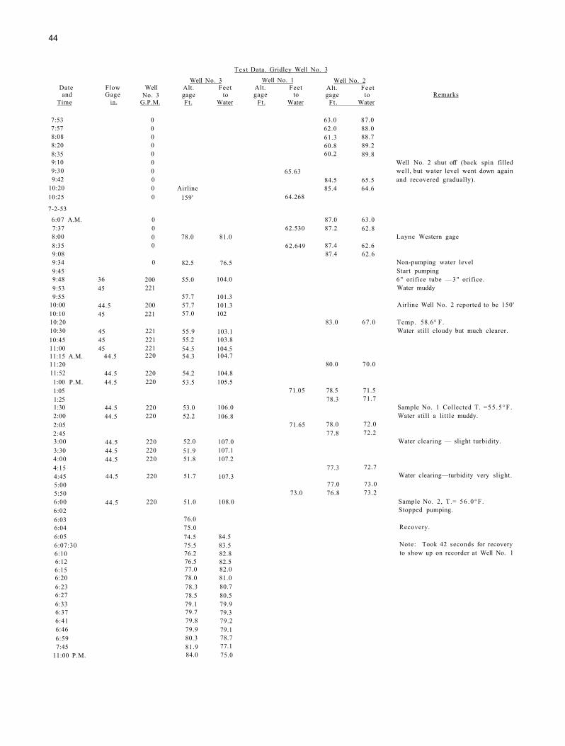
44

Tes t Data. Gridley Well No. 3

Well No. 3 Well No. 1 Well No. 2 Date Flow Well Alt. Feet Alt. Feet Alt. Feet and Gage No. 3 gage to gage to gage to Remarks

Time i n . G.P.M. Ft . Water Ft. Water Ft . Water

7:53 0 63.0 87.0 7:57 0 62.0 88.0 8:08 0 61.3 88.7 8:20 0 60.8 89.2 8:35 0 60.2 89.8 9:10 0 Well No. 2 shut off (back spin filled 9:30 0 65.63 well, but water level went down again 9:42 0 84.5 65.5 and recovered gradually).

10:20 0 Airline 85.4 64.6 10:25 0 159' 64.268

7-2-53

6:07 A.M. 0 87.0 63.0 7:37 0 62.530 87.2 62.8 8:00 0 78.0 81.0 Layne Western gage 8:35 0 62.649 87.4 62.6 9:08 87.4 62.6 9:34 0 82.5 76.5 Non-pumping water level 9:45 Start pumping 9:48 36 200 55.0 104.0 6" orifice tube — 3 " orifice. 9:53 45 221 Water muddy 9:55 57.7 101.3

10:00 44.5 200 57.7 101.3 Airline Well No. 2 reported to be 150' 10:10 45 221 57.0 102 10:20 83.0 67.0 Temp. 58.6° F. 10:30 45 221 55.9 103.1 Water still cloudy but much clearer. 10:45 45 221 55.2 103.8 11:00 45 221 54.5 104.5 11:15 A.M. 44.5 220 54.3 104.7 11:20 80.0 70.0 11:52 44.5 220 54.2 104.8 1:00 P.M. 44.5 220 53.5 105.5 1:05 71.05 78.5 71.5 1:25 78.3 71.7 1:30 44.5 220 53.0 106.0 Sample No. 1 Collected T. =55 .5°F . 2:00 44.5 220 52.2 106.8 Water still a little muddy. 2:05 71.65 78.0 72.0 2:45 77.8 72.2 3:00 44.5 220 52.0 107.0 Water clearing — slight turbidity. 3:30 44.5 220 51.9 107.1 4:00 44.5 220 51.8 107.2 4:15 77.3 72.7 4:45 44.5 220 51.7 107.3 Water clearing—turbidity very slight. 5:00 77.0 73.0 5:50 73.0 76.8 73.2 6:00 44.5 220 51.0 108.0 Sample No. 2, T.= 56 .0°F . 6:02 Stopped pumping. 6:03 76.0 6:04 75.0 Recovery. 6:05 74.5 84.5 6:07:30 75.5 83.5 Note: Took 42 seconds for recovery 6:10 76.2 82.8 to show up on recorder at Well No. 1 6:12 76.5 82.5 6:15 77.0 82.0 6:20 78.0 81.0 6:23 78.3 80.7 6:27 78.5 80.5 6:33 79.1 79.9 6:37 79.7 79.3 6:41 79.8 79.2 6:46 79.9 79.1 6:59 80.3 78.7 7:45 81.9 77.1

11:00 P.M. 84.0 75.0

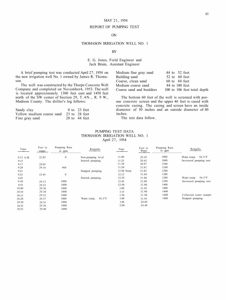
45

MAY 21, 1954

REPORT OF PUMPING TEST

ON

THOMASON IRRIGATION WELL NO. 1

BY

E. G. Jones, Field Engineer and Jack Bruin, Assistant Engineer

A brief pumping test was conducted April 27, 1954 on the new irrigation well No. 1 owned by James R. Thoma-son.

The well was constructed by the Thorpe Concrete Well Company and completed on November4, 1953. The well is located approximately 1300 feet east and 1450 feet north of the SW comer of Section 29, T . 4 N . , R. 9 W., Madison County. The driller's log follows:

Sandy clay 0 to 23 feet Yellow medium coarse sand 23 to 28 feet Fine gray sand 28 to 44 feet

Medium fine gray sand 44 to 52 feet Building sand 52 to 60 feet Coarse, clean sand 60 to 84 feet Medium coarse sand 84 to 100 feet Coarse sand and boulders 100 to 106 feet total depth

The bottom 60 feet of the well is screened with por­ous concrete screen and the upper 46 feet is cased with concrete casing. The casing and screen have an inside diameter of 30 inches and an outside diameter of 40 inches.

The test data follow.

PUMPING TEST DATA THOMASON IRRIGATION WELL NO. 1

April 27, 1954

Time Feet to water

Pumping Rate in gpm

Remarks Time Feet to Water

Pumping Rate in gpm Remarks

9:13 A.M. 23.95 0 Non-pumping level 11:00 29.39 1000 Water temp. 56.5°F 9:15 Started pumping 11:25 29.43 1000 Increased pumping rate 9:17 29.03 11:30 30.97 1280 9:20 29.16 960 11:50 31.01 1280 9:21 Stopped pumping 12:00 Noon 31.02 1280 9:23 23.95 0 12:15 31.04 1280 9:45 Started pumping 12:30 31.08 1280 Water temp. 56.5°F 9:50 29.13 1000 12:45 31.08 1280 Increased pumping rate 9:55 29.23 1000 12:50 31.90 1400

10:00 29.30 1000 1:00 31.95 1400 10:10 29.30 1000 1:15 31.90 1400 10:15 29.32 1000 1:30 31.90 1400 Collected water sample 10:20 29.37 1000 Water temp. 56.5°F 1:40 31.93 1400 Stopped pumping 10:30 29.35 1000 1:44 24.60 10:35 29.36 1000 2:00 24.40 10:52 29.40 1000

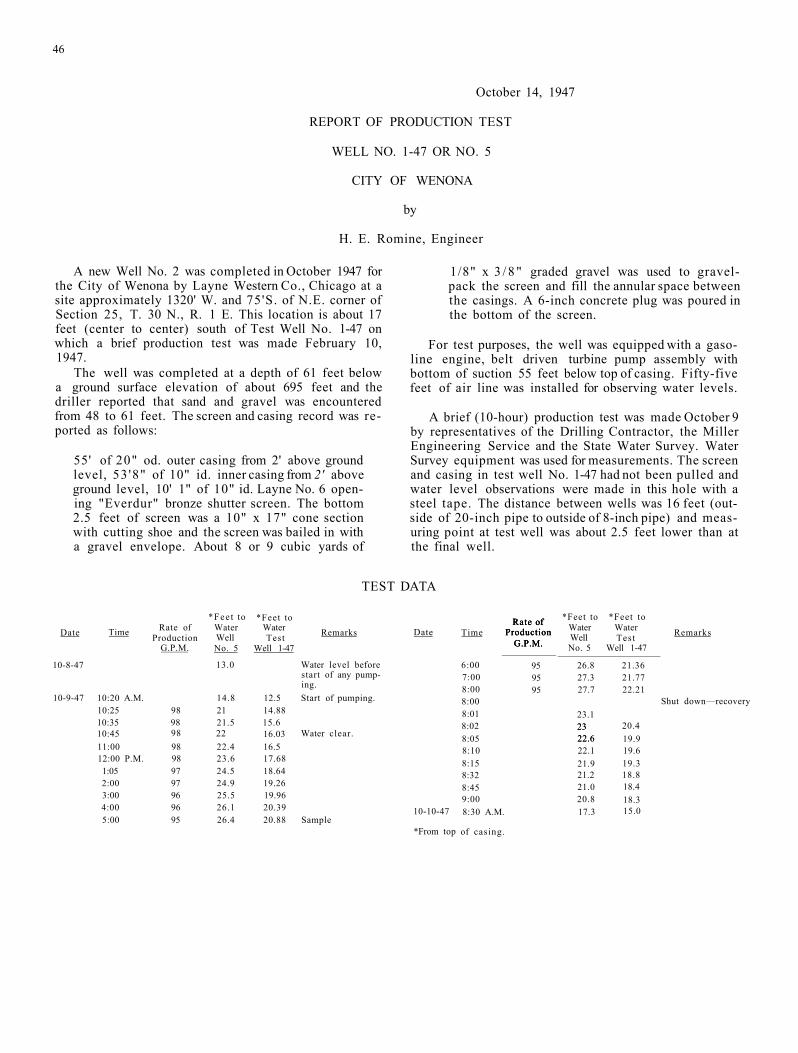
46

October 14, 1947

REPORT OF PRODUCTION TEST

WELL NO. 1-47 OR NO. 5

CITY OF WENONA

by

H. E. Romine, Engineer

A new Well No. 2 was completed in October 1947 for the City of Wenona by Layne Western Co., Chicago at a site approximately 1320' W. and 75'S. of N.E. corner of Section 25, T. 30 N., R. 1 E. This location is about 17 feet (center to center) south of Test Well No. 1-47 on which a brief production test was made February 10, 1947.

The well was completed at a depth of 61 feet below a ground surface elevation of about 695 feet and the driller reported that sand and gravel was encountered from 48 to 61 feet. The screen and casing record was re­ported as follows:

55' of 20" od. outer casing from 2' above ground level, 53 '8" of 10" id. inner casing from 2' above ground level, 10' 1" of 10" id. Layne No. 6 open­ing "Everdur" bronze shutter screen. The bottom 2.5 feet of screen was a 10" x 17" cone section with cutting shoe and the screen was bailed in with a gravel envelope. About 8 or 9 cubic yards of

1/8" x 3 / 8 " graded gravel was used to gravel-pack the screen and fill the annular space between the casings. A 6-inch concrete plug was poured in the bottom of the screen.

For test purposes, the well was equipped with a gaso­line engine, belt driven turbine pump assembly with bottom of suction 55 feet below top of casing. Fifty-five feet of air line was installed for observing water levels.

A brief (10-hour) production test was made October 9 by representatives of the Drilling Contractor, the Miller Engineering Service and the State Water Survey. Water Survey equipment was used for measurements. The screen and casing in test well No. 1-47 had not been pulled and water level observations were made in this hole with a steel tape. The distance between wells was 16 feet (out­side of 20-inch pipe to outside of 8-inch pipe) and meas­uring point at test well was about 2.5 feet lower than at the final well.

TEST DATA

*Fee t to *Feet to Rate of Production

G.P.M.

*Feet to *Feet to

Date Time Rate of Production

Water Well

Water Test Remarks Date Time

Rate of Production

G.P.M.

Water Well

Water Test Remarks

G.P.M. No. 5 Well 1-47

Rate of Production

G.P.M. No. 5 Well 1-47

10-8-47 13.0 Water level before start of any pump­ing.

6:00 7:00 8:00

95 95 95

26.8 27.3 27.7

21.36 21.77 22.21

10-9-47 10:20 A.M. 14.8 12.5 Start of pumping. 8:00 Shut down—recovery 10:25 98 21 14.88 8:01 23.1 10:35 98 21.5 15.6 8:02 23

22.6 20.4

10:45 98 22 16.03 Water clear. 8:05 23 22.6 19.9

11:00 98 22.4 16.5 8:10 22.1 19.6 12:00 P.M. 98 23.6 17.68 8:15 21.9 19.3 1:05 97 24.5 18.64 8:32 21.2 18.8 2:00 97 24.9 19.26 8:45 21.0 18.4 3:00 96 25.5 19.96 9:00 20.8 18.3 4:00 96 26.1 20.39 10-10-47 8:30 A.M. 17.3 15.0 5:00 95 26.4 20.88 Sample

*From top of casing.

47

APPENDIX II

SUGGESTIONS FOR CONDUCTING WATER-WELL PUMPING TESTS

49

APPENDIX II

SUGGESTIONS FOR CONDUCTING

WATER-WELL PUMPING TESTS

INTRODUCTION

This circular is prepared for the use of well drillers and engineers who conduct water-well pumping tests in the State of Illinois. It is a general discussion of some of the factors which should be considered before starting a pumping test.

There are no specific rules proposed which apply to all tests but the following suggestions fit most cases:

1. All significant data which can be economically collected should be recorded in a neat and legible form.

2. All measurements should be made with precision consistent with the required accuracy of results where costs are not prohibitive.

Each pumping test is conducted under certain prevail­ing conditions, and it cannot be assumed that these con­ditions are ever identical in any two tests. Because of the uncertainties and variable factors involved there is no substitute for the service of competent persons experi­enced in pumping-test work.

THE PUMPED WELL

1. If the well to be tested produces water from sand and gravel, the screen should be of maximum practicable length and diameter. It should be selected with care to fit the graduation of sand and gravel encountered. Unless the well is of the gravel-pack type, the finer material surrounding the well should be loosened, drawn through the screen by surging and removed from the well before the test pump is installed.

2. The pump should be installed and a preliminary test run to see whether the formation is worthy of a more detailed and prolonged production test.

3. The preliminary production test will reveal wheth­er or not the pump is set deep enough. Any necessary changes can be made before the date of the test.

4. An air line of known length constructed of some suitable material should be installed in the pumped well with the lower end near the top of the pump-bowl section or a foot or two above the lower end of the pump-suction pipe. The upper end of the air line should be equipped with a ¼-inch pipe tee. An ordinary tire-valve stem equipped with a valve core should be installed in the tee. The air gage should be connected to the other open­ing of the pipe tee. The air-line system should be en­tirely free of air leaks except for the open end at the bottom. An ordinary tire pump should also be available.

When an air line is not available, provision must be made for lowering an electric dropline or other water-level measuring device into the well. This requires a free passageway into the annular space between the well cas­

ing or hole and the pump column pipe. The annular space between the well casing and pump column pipe must be of sufficient dimension to allow free passage of the water-level measuring device up and down the well. Figure 1 shows some of the devices now being used to measure water levels manually.

FIG. 1. MANUAL WATER LEVEL MEASURING DEVICES

Figure 2 is a sketch of a typical test "set-up" on the pumped well.

FIG. 2. TYPICAL SET-UP FOR WELL PRODUCTION TEST

50

PUMPING EQUIPMENT

Pump. A turbine-type pump is preferable to a plunger or rig-operated pump in all cases. The pump should have sufficient capacity to pump at least the maximum de­sired rate in the case of a finished well.

Power. Either an electric motor or some type of in­ternal combustion engine may be used to run the pump. A steam engine is not satisfactory because of the diffi­culty in maintaining uniform speed. More precise data can usually be obtained when an electric motor is used.

The pumping equipment should be capable of oper­ating continuously for the entire period of the test. In­ternal combustion enginees must be in good condition in order to meet this requirement.

Discharge Piping. The pump discharge line should be equipped with a valve so that the rate of discharge may be accurately controlled. Provision must be made for the installation of orifice plates and piezometer tube (as shown in Figure 1) or other acceptable equipment to measure the pumping rate. At the beginning of the test the valve should be partially closed to enable adjustment in the rate as the test progresses.

OBSERVATION WELLS

When the purpose of the pumping test is to evaluate well interference or the characteristics of the water-producing formation, it is necessary to have one or more observation wells. The observation wells should be lo­cated in the vicinity of, and at various distances from, the pumped well. The tops of the observation wells should be accessible so that water-level recorders or other mea­suring equipment may be installed.

If wells are drilled to be used only as observation wells they should be at least 1¼ inches in diameter when water-level measurements are to be made with a tape or elec­tric dropline. If float-actuated water-level recorders are to be used, it is desirable to have observation wells at least 6 inches in diameter.

The distances between all wells should be carefully measured and reference elevations determined. When­ever possible, the logs of all wells should be made avail­able prior to the test.

When the observation well is a well with a permanent pump installed, the well must be equipped with an air line of known length.

PERIOD PRIOR TO TEST

In order to obtain the most reliable data, the water-producing formation should be hydraulically stable prior to the test (i.e. the water levels should not be changing). This condition can usually be approached by discontin­uing all pumping from the water-producing formation for a period of time. This period should usually be at least 24 hours but may vary considerably with different forma­tions. After pumping is stopped (in preparation for the test) water levels should be measured periodically. Not until constancy has been observed should the test be started.

Where it is impractical to stop all pumping from other wells in the vicinity, these wells should be kept pumping

at constant rates for the period prior to and during the test.

It is not always possible to meet these conditions, but every effort should be made to adhere to them as nearly as possible, otherwise the reliability of the data will suffer.

NOTES CONCERNING COLLECTION OF DATA Pumping Rates. During the early part of a pumping

test the water level in the pumped well lowers rapidly. This increases the net pumping head and will usually cause the pumping rate to decrease appreciably. The pumping rate should be checked continuously during this part of the test and the discharge valve manipulated to keep the pumping rate as nearly constant as possible. As the test progresses the rate of lowering of the water level ordinarily decreases and it is not necessary to check the pumping rate quite so closely. However, the importance of keeping the pumping rate under close control through­out the test cannot be overemphasized.

Atmospheric conditions such as the temperature and humidity of the air may appreciably affect the operation of the prime mover and thus cause variations in the pump­ing rate. This is particularly true when the pump is driven by an internal combustion engine. Variations in line volt­age can affect the pumping rate when the prime mover is an electric motor. In view of such facts as these, it is important to keep a rather close check on the pumping rate throughout the test.

Any appreciable variations in pumping rate should al­ways be recorded and the cause noted when it can be determined.

Water Levels. Because of the head characteristics of pumps, any factor which affects the pumping rate will also have some effect on the water level and vice versa.

Changes in barometric pressure may cause the water levels to fluctuate in some artesian wells. A rise in baro­metric pressure would cause a lowering of water level. It is very seldom that barometric pressure changes during a pumping test would cause water-level variations of more than one foot, and the change is usually much less.

As mentioned previously, the water levels may be in­fluenced by pumping from other wells in the area.

Frequency of Observations. The frequency of obser­vations and the amount of data recorded will vary with the accuracy desired of the results, the available per­sonnel, and the particular well and water-bearing for­mation being tested.

Ordinarily it is desirable to make observations more frequently during the earlier part of the test and to in­crease the period between observations as the test pro­gresses. After pumping has been stopped, measurements of the water-level recovery should be made quite fre­quently during the earlier part of the recovery period. There is often a tendency on the part of the observers to neglect the measurement of recovery. This is unfor­tunate because sometimes the data obtained from re­covery measurements are extremely important.

In general when the water level is changing rapidly, readings should be taken as often as they can be recorded. As the water level becomes more steady, sufficient read­ings should be taken to facilitate a well-defined curve

51

on a graph of water levels versus elapsed time. Table 1 is a tabulation of data collected from an ac­

tual pumping test. This example may be used as a general guide for the frequency of observations. It is also a con­venient form in which to record the test data.

TYPES OF PUMPING TESTS

Two types of tests are commonly used in Illinois. The "constant-rate" test is usually used when observation wells are available and the purpose of the test is to de­termine the characteristics of the aquifer. In this case, the well is pumped at a constant rate for the entire pe­riod of the test. The "step draw-down" test is usually

conducted to determine the characteristics of the well itself. Pumping is started at a low rate and increased at regular intervals until the desired capacity or the maxi­mum capacity of the well is obtained.

The necessary length of test for the "constant-rate" test and the necessary pumping period at each rate of the "step draw-down" test will vary from case to case. A competent person experienced in pumping-test work can usually estimate the necessary length of test from an ex­amination of the preliminary test data. However, this would be only an estimate, and events which take place during the test itself may make it highly desirable to extend, shorten, or entirely change the whole test pro­cedure.

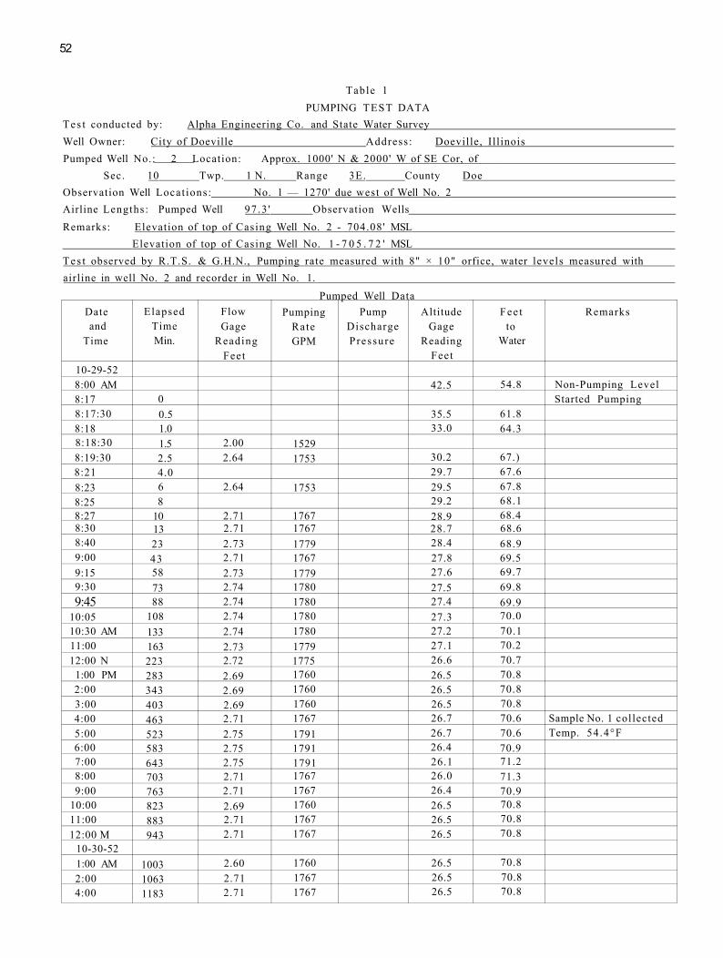
52

Table 1 PUMPING TEST DATA

Tes t conducted by: Alpha Engineering Co. and State Water Survey Well Owner: City of Doeville Address : Doeville, Illinois Pumped Well No.: 2 Location: Approx. 1000' N & 2000' W of SE Cor, of

Sec. 10 Twp. 1 N. Range 3E. County Doe Observation Well Locat ions: No. 1 — 1270' due west of Well No. 2 Airline Lengths: Pumped Well 97 .3 ' Observation Wells Remarks: Elevation of top of Casing Well No. 2 - 704.08' MSL

Elevation of top of Casing Well No. 1 - 7 0 5 . 7 2 ' MSL Tes t observed by R.T.S. & G.H.N., Pumping rate measured with 8" × 10" orfice, water levels measured with airline in well No. 2 and recorder in Well No. 1.

Pumped Well Data Date and

Time

Elapsed Time Min.

Flow Gage

Reading Feet

Pumping Rate GPM

Pump Discharge Pressure

Altitude Gage

Reading Feet

Fee t to

Water

Remarks

10-29-52 8:00 AM 42.5 54.8 Non-Pumping Level 8:17 0 Started Pumping 8:17:30 0.5 35.5 61.8 8:18 1.0 33.0 64.3 8:18:30 1.5 2.00 1529 8:19:30 2.5 2.64 1753 30.2 67.) 8:21 4.0 29.7 67.6 8:23 6 2.64 1753 29.5 67.8 8:25 8 29.2 68.1 8:27 10 2.71 1767 28.9 68.4 8:30 13 2.71 1767 28.7 68.6 8:40 23 2.73 1779 28.4 68.9 9:00 43 2.71 1767 27.8 69.5 9:15 58 2.73 1779 27.6 69.7 9:30 73 2.74 1780 27.5 69.8 9:45 88 2.74 1780 27.4 69.9

10:05 108 2.74 1780 27.3 70.0 10:30 AM 133 2.74 1780 27.2 70.1 11:00 163 2.73 1779 27.1 70.2 12:00 N 223 2.72 1775 26.6 70.7

1:00 PM 283 2.69 1760 26.5 70.8 2:00 343 2.69 1760 26.5 70.8 3:00 403 2.69 1760 26.5 70.8 4:00 463 2.71 1767 26.7 70.6 Sample No. 1 collected 5:00 523 2.75 1791 26.7 70.6 Temp. 54.4°F 6:00 583 2.75 1791 26.4 70.9 7:00 643 2.75 1791 26.1 71.2 8:00 703 2.71 1767 26.0 71.3 9:00 763 2.71 1767 26.4 70.9

10:00 823 2.69 1760 26.5 70.8 11:00 883 2.71 1767 26.5 70.8 12:00 M 943 2.71 1767 26.5 70.8

10-30-52 1:00 AM 1003 2.60 1760 26.5 70.8 2:00 1063 2.71 1767 26.5 70.8 4:00 1183 2.71 1767 26.5 70.8

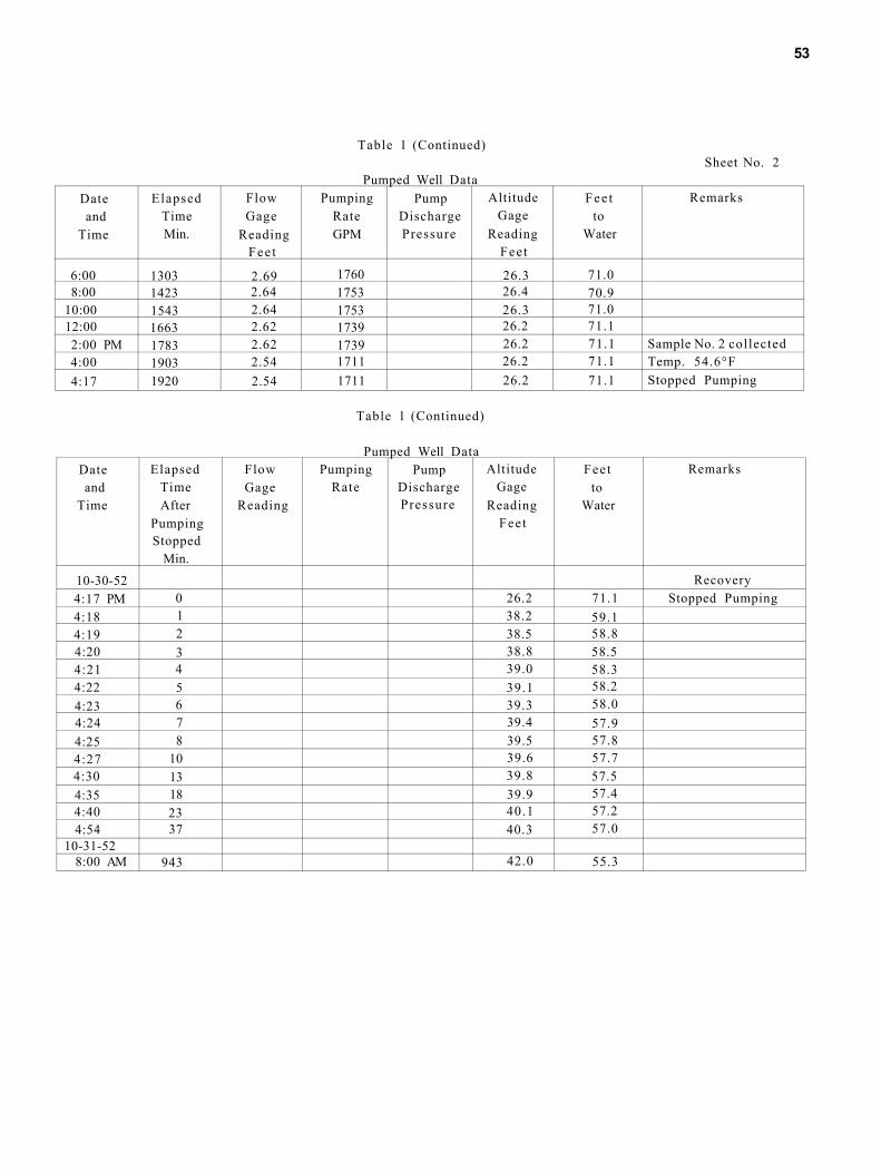
Table 1 (Continued) Sheet No. 2

Pumped Well Data Date and

Time

Elapsed Time Min.

Flow Gage

Reading Fee t

Pumping Rate GPM

Pump Discharge Pressure

Altitude Gage

Reading Fee t

Fee t to

Water

Remarks

6:00 1303 2.69 1760 26.3 71.0 8:00 1423 2.64 1753 26.4 70.9

10:00 1543 2.64 1753 26.3 71.0 12:00 1663 2.62 1739 26.2 71.1 2:00 PM 1783 2.62 1739 26.2 71.1 Sample No. 2 collected 4:00 1903 2.54 1711 26.2 71.1 Temp. 54.6°F 4:17 1920 2.54 1711 26.2 71.1 Stopped Pumping

Table 1 (Continued)

Pumped Well Data Date and

Time

Elapsed Time After

Pumping Stopped

Min.

Flow Gage

Reading

Pumping Rate

Pump Discharge Pressure

Altitude Gage

Reading Fee t

Fee t to

Water

Remarks

10-30-52 Recovery 4:17 PM 0 26.2 71.1 Stopped Pumping 4:18 1 38.2 59.1 4:19 2 38.5 58.8 4:20 3 38.8 58.5 4:21 4 39.0 58.3 4:22 5 39.1 58.2 4:23 6 39.3 58.0 4:24 7 39.4 57.9 4:25 8 39.5 57.8 4:27 10 39.6 57.7 4:30 13 39.8 57.5 4:35 18 39.9 57.4 4:40 23 40.1 57.2 4:54 37 40.3 57.0

10-31-52 8:00 AM 943 42.0 55.3

53

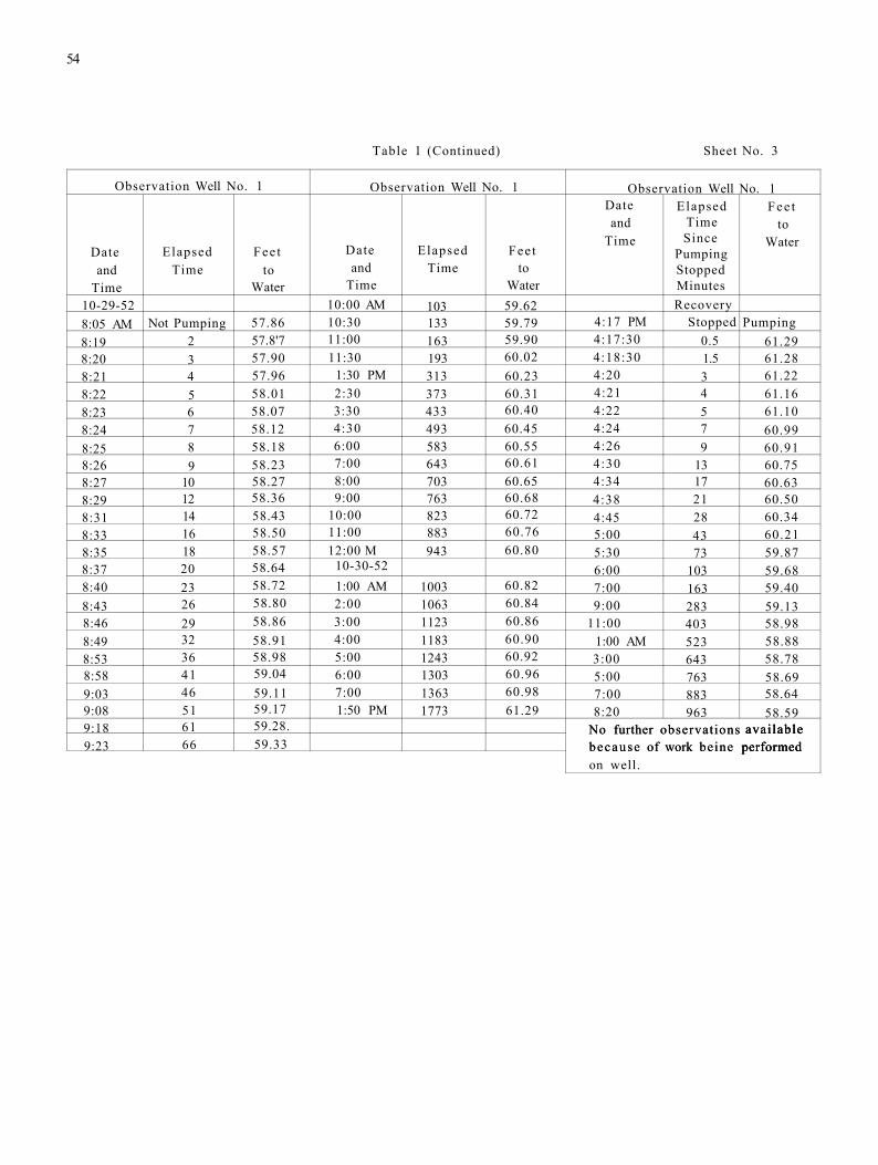
54

Table 1 (Continued) Sheet No. 3

Observation Well No. 1 Observation Well No. 1 Observation Well No. 1

Date and

Time

Elapsed Time

Feet to

Water

Date and

Time

Elapsed Time

Feet to

Water

Date and

Time

Elapsed Time Since

Pumping Stopped Minutes

Fee t to

Water

10-29-52 10:00 AM 103 59.62 Recovery 8:05 AM Not Pumping 57.86 10:30 133 59.79 4:17 PM Stopped Pumping 8:19 2 57.8'7 11:00 163 59.90 4:17:30 0.5 61.29 8:20 3 57.90 11:30 193 60.02 4:18:30 1.5 61.28 8:21 4 57.96 1:30 PM 313 60.23 4:20 3 61.22 8:22 5 58.01 2:30 373 60.31 4:21 4 61.16 8:23 6 58.07 3:30 433 60.40 4:22 5 61.10 8:24 7 58.12 4:30 493 60.45 4:24 7 60.99 8:25 8 58.18 6:00 583 60.55 4:26 9 60.91 8:26 9 58.23 7:00 643 60.61 4:30 13 60.75 8:27 10 58.27 8:00 703 60.65 4:34 17 60.63 8:29 12 58.36 9:00 763 60.68 4:38 21 60.50 8:31 14 58.43 10:00 823 60.72 4:45 28 60.34 8:33 16 58.50 11:00 883 60.76 5:00 43 60.21 8:35 18 58.57 12:00 M 943 60.80 5:30 73 59.87 8:37 20 58.64 10-30-52 6:00 103 59.68 8:40 23 58.72 1:00 AM 1003 60.82 7:00 163 59.40 8:43 26 58.80 2:00 1063 60.84 9:00 283 59.13 8:46 29 58.86 3:00 1123 60.86 11:00 403 58.98 8:49 32 58.91 4:00 1183 60.90 1:00 AM 523 58.88 8:53 36 58.98 5:00 1243 60.92 3:00 643 58.78 8:58 41 59.04 6:00 1303 60.96 5:00 763 58.69 9:03 46 59.11 7:00 1363 60.98 7:00 883 58.64 9:08 51 59.17 1:50 PM 1773 61.29 8:20 963 58.59 9:18 61 59.28. No further observations

because of work beine available

performed 9:23 66 59.33 No further observations because of work beine

available performed

on well.

available performed